Superparameterised cloud effects in the EMAC general circulation model (v2.50) – influences of model configuration

A new module has been implemented in the fifth generation of the ECMWF/Hamburg (ECHAM5)/Modular Earth Submodel System (MESSy) Atmospheric Chemistry (EMAC) model that simulates cloud-related processes on a much smaller grid. This so-called superparameterisation acts as a replacement for the convection parameterisation and large-scale cloud scheme. The concept of embedding a cloud-resolving model (CRM) inside of each grid box of a general circulation model leads to an explicit representation of cloud dynamics.

The new model component is evaluated against observations and the conventional usage of EMAC using a convection parameterisation. In particular, effects of applying different configurations of the superparameterisation are analysed in a systematical way. Consequences of changing the CRM's orientation, cell size and number of cells range from regional differences in cloud amount up to global impacts on precipitation distribution and its variability. For some edge case setups, the analysed climate state of superparameterised simulations even deteriorates from the mean observed energy budget.

In the current model configuration, different climate regimes can be formed that are mainly driven by some of the parameters of the CRM. Presently, the simulated total cloud cover is at the lower edge of the CMIP5 model ensemble. However, certain “tuning” of the current model configuration could improve the slightly underestimated cloud cover, which will result in a shift of the simulated climate.

The simulation results show that especially tropical precipitation is better represented with the superparameterisation in the EMAC model configuration. Furthermore, the diurnal cycle of precipitation is heavily affected by the choice of the CRM parameters. However, despite an improvement of the representation of the continental diurnal cycle in some configurations, other parameter choices result in a deterioration compared to the reference simulation using a conventional convection parameterisation.

The ability of the superparameterisation to represent latent and sensible heat flux climatology is independent of the chosen CRM setup. Evaluation of in-atmosphere cloud amounts depending on the chosen CRM setup shows that cloud development can significantly be influenced on the large scale using a too-small CRM domain size. Therefore, a careful selection of the CRM setup is recommended using 32 or more CRM cells to compensate for computational expenses.

1 Introduction

Cloud-related processes are difficult to simulate on the coarse grid of a general circulation model (GCM) and have a substantial influence on the global climate (Boucher et al., 2013). Small-scale effects like deep convection need to be parameterised in global models, uncovering the problem that Earth system model (ESM) horizontal grid spacing requires further refinement to resolve cloud formation. Uncertainties in different atmospheric fields are primarily a consequence of using parameterisations (Zhang and McFarlane, 1995; Knutti et al., 2002), which rely on a physical basis but are mostly scale dependent including an arbitrary number of simplifications and assumptions. Nowadays, computational capabilities are suitable to perform global or large-domain simulations with resolution on the order of a few kilometres (Kajikawa et al., 2016; Heinze et al., 2017a) or even sub-kilometre grid spacing (Miyamoto et al., 2013). Convective-permitting simulations have shown that these models are able to realistically represent the Madden–Julian oscillation (MJO) (Miura et al., 2007; Miyakawa et al., 2014), the diurnal cycle of precipitation (Sato et al., 2009; Yashiro et al., 2016) or the monsoon onset (Kajikawa et al., 2015). Resolving the total effects of small-scale atmospheric features can hardly be simulated by any GCM with parameterised physics. The dilemma with these global cloud-resolving models (GCRMs) is the simulation period that is limited by the computational expense to a couple of months nowadays. On that account, coarser horizontal resolutions are necessary regarding long-term simulations, e.g. climate projections. A pioneer high-resolution (14 km global mesh) multi-year climate simulations has been conducted by Kodama et al. (2015). In addition to that, the first coordinated long-term model intercomparison of high-resolution (at least 50 km grid size) climate simulations is under way within the High Resolution Model Intercomparison Project (HighResMIP) (Haarsma et al., 2016) of the sixth phase of the Coupled Model Intercomparison Project (CMIP6) (Eyring et al., 2016). The former examples showed that current developments and models still use resolutions that require a convection parameterisation in order to investigate climate-related questions. Combining the ability to reproduce small-scale cloud dynamics by a cloud-resolving model (CRM) and perform long-term simulations with a GCM resulted in the idea of a “superparameterisation” (Grabowski and Smolarkiewicz, 1999; Grabowski, 2001; Khairoutdinov and Randall, 2001).

The concept of the superparameterisation is based on embedding a CRM inside of each column of the GCM replacing convection and large-scale cloud parameterisations. The superparameterisation acts as a conventional parameterisation but in contrast explicitly resolving small-scale cloud dynamics on the subgrid-scale of the GCM with the exception of cloud microphysics and turbulence. The CRM domain involves periodic lateral boundary conditions and forcings of large-scale tendencies, computed by the GCM, that are applied as horizontally uniform. Finally, all small-scale effects represented by the mean of all CRM columns within one GCM grid box interact with larger-scale atmosphere circulations on the coarse grid of the host model. Consequently, no direct interactions between individual CRM cells across GCM grid boundaries are possible. The computational cost of performing simulations with this framework is drastically reduced in contrast to a fully global cloud-resolving model (Grabowski, 2016). Including a CRM for the representation of the multitude of different types of clouds is a major step toward a more realistic representation of individual clouds and their interactions that are otherwise only achievable with high-resolution models over huge domains.

After the first implementation of the superparameterisation, several other institutes have followed the same approach (Subramanian et al., 2017; Tulich, 2015; Tao et al., 2009) and others are under way (Arakawa et al., 2011). Nowadays, state-of-the-art global cloud-resolving models provide new possibilities, comparing superparameterised simulations with month-long high-resolution models (Stevens et al., 2019). In addition to this, the Center for Multiscale Modeling of Atmospheric Processes (CMMAP) has been created as a National Science Foundation's Science and Technology Center extensively progressing the work with superparameterisations (Randall et al., 2003; Randall, 2013; Khairoutdinov and Randall, 2006; Wyant et al., 2009; Elliott et al., 2016). Diverse modifications exist, which incorporate other processes or schemes within the embedded small-scale model, like a two-moment microphysical scheme (Morrison et al., 2009), a higher-order turbulence closure or including aerosol coupling (Gustafson et al., 2008; Cheng and Xu, 2013; Wang et al., 2011a, b; Minghuai et al., 2015). These studies have mainly focused on improving selected process descriptions within the cloud-resolving model. This study presents an additional superparameterised GCM, primarily focusing on the effects of different CRM model configurations onto the mean climate state. Multiple simulations spanning 15 months have been performed to statistically evaluate the effects of changing different aspects of the superparameterisation, i.e. orientation, grid spacing and cell number of the embedded CRM. To our knowledge, this is the first attempt at summarising the effects of different configurations of the superparameterisation onto the model mean climate state.

This paper is organised as follows. Section 2 describes the host GCM and CRM that are used as the superparameterisation. Furthermore, the coupling between the two model systems and the simulation setup is given. Section 3 examines the results of the new model system and discusses the sensitivity study comparing different superparameterised model setups. Section 4 gives a summary and conclusions.

Table 1 Overview of sensitivity simulations.

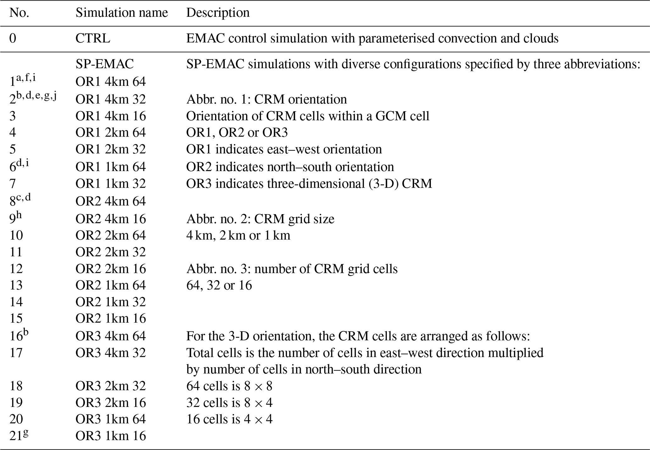
Configurations that have been used in previous literature: ^a Khairoutdinov and Randall (2001). ^b Khairoutdinov et al. (2005). ^c Khairoutdinov et al. (2008). ^d Kooperman et al. (2013). ^e Kooperman et al. (2014). ^f Cole et al. (2005). ^g Parishani et al. (2017). ^h Pritchard et al. (2014). ⁱ Marchand and Ackerman (2010). ^j Wang et al. (2011a).

2 Model description

2.1 EMAC model system

Historically speaking, the ECHAM/Modular Earth Submodel System (MESSy) Atmospheric Chemistry (EMAC) model (Joeckel et al., 2010) combines the MESSy framework with the fifth generation of the ECMWF/Hamburg (ECHAM5) climate model (Roeckner et al., 2006). Developments during the last decade have fully modularised the code into the different layers of MESSy (Joeckel et al., 2005) and split representations of atmospheric processes into their own submodels. Based on that, alternative process descriptions (e.g. convection parameterisations; Tost et al., 2006) and even diverse base models (e.g. Community Earth System Model – CESM, Baumgaertner et al., 2016, or the COSMO model, Kerkweg and Jöckel, 2012) can be easily selected and compared for sensitivity climate simulations. EMAC has been used for various scientific applications regarding chemistry–climate interactions from the surface to the mesosphere¹. A complete list of available submodels is given in Table 1 in Joeckel et al. (2010).

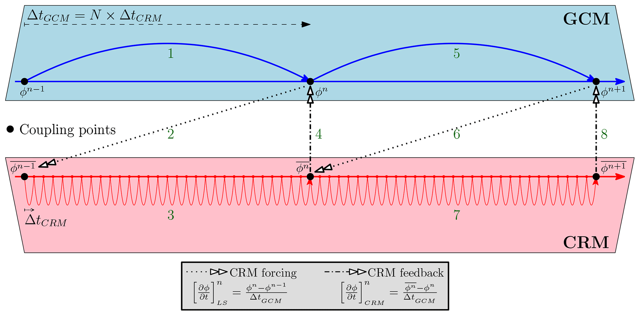
Figure 1 Sketch of model time integration when coupling a host GCM with a superparameterisation (i.e. CRM) based on their prognostic variables ϕ over a period of two time steps (n). A description of the different phases (i.e. numbers) is given in the text.

2.2 New submodule: CRM

As mentioned in the introduction, a CRM has been implemented as a new submodel to serve as a superparameterisation (SP) for EMAC. The new coupled model system is therefore shortly named SP-EMAC. The CRM component of SP-EMAC is the System for Atmospheric Modeling (SAM; described in Khairoutdinov and Randall, 2003) that describes subgrid-scale development of moist physics in each GCM grid column. It solves the non-hydrostatic dynamical equations with the anelastic approximation. The prognostic variables are the liquid/ice water moist static energy, total precipitating water (rain plus snow plus graupel) and non-precipitating water (vapour plus cloud water plus cloud ice). An “all-or-nothing” approach is used to diagnose cloud condensation assuming saturation with respect to water/ice. The hydrometeor partitioning is based on a temperature dependence using a single-moment microphysical scheme with fixed autoconversion rates. Additional information on the CRM is described in more detail in the Appendix of Khairoutdinov and Randall (2003).

The model code of the superparameterisation has been restructured to follow the MESSy coding standards. Thereby, it is now possible to set specific parameters via namelist entries in order to obtain the flexibility for sensitivity analysis without recompiling the code. The main switches that can be adjusted change the configuration of the superparameterisation, i.e.

• number of CRM grid cells inside of each GCM grid box;

• grid size of CRM cells;

• orientation of the CRM columns (2-D or 3-D);

• top height of CRM grid box; and

• time step of the superparameterisation.

Each grid column of the global model EMAC hosts several copies of the CRM. All configurations of the superparameterisation use periodical lateral boundaries and a time step of 20 s. Vertical levels (29 in total) are aligned to match the lowermost levels of the GCM. Newtonian damping is applied to all prognostic variables in the upper third of the grid to reduce gravity wave reflection and build-up. Communication between CRM cells across GCM boundaries is done via large-scale tendencies, thereby neglecting direct interactions of small-scale dynamics between coarse grid columns.

2.3 SP-EMAC: coupling the two model systems

Combining EMAC and the superparameterisation is based on applying the CRM forcing and CRM feedback of prognostic variables ϕ between the two models. But first and foremost, vertical profiles of the coarse grid cells of EMAC are initialised in all CRM columns at the beginning of each model run. Simultaneously, small temperature perturbations are added for near-surface layers to obtain an individual response for each CRM column. During the simulation, the CRM is called on every GCM time step and repeatedly integrating its equations while saving all subgrid-scale fields of the superparameterisation at the end of the call. A sketch of the GCM-CRM coupling is given in Fig. 1 displaying two GCM time steps (n) and their sequential phases during the model time integration. The numbers in Fig. 1 correspond to the following actions:

• 1.

  integration of GCM (time step of Δt_GCM);

• 2.

  coupling: CRM large-scale forcing ${\left[\frac{\partial \mathit{\varphi }}{\partial t}\right]}_{\mathrm{LS}}$;

• 3.

  integration of CRM (N multiplied by Δt_CRM); and

• 4.

  coupling: CRM small-scale feedback ${\left[\frac{\partial \mathit{\varphi }}{\partial t}\right]}_{\mathrm{CRM}}$.

The large-scale forcing ${\left[\frac{\partial \mathit{\varphi }}{\partial t}\right]}_{\mathrm{LS}}^n$ restricts the superparameterisation close to the host model fields, whereas CRM feedback ${\left[\frac{\partial \mathit{\varphi }}{\partial t}\right]}_{\mathrm{CRM}}^n$ tendencies are calculated by the horizontal mean of all CRM grid boxes ($\stackrel{\mathrm{‾}}{{\mathit{\varphi }}^n}$) for time step n (Grabowski, 2004b). Prognostic variables that have been coupled are temperature and moisture in terms of water vapour, cloud water and cloud ice. Horizontal momentum transport was only allowed for the 3-D CRM configurations applying the same relaxation terms (see Fig. 1) to the u and v wind field components. All 2-D CRM configurations neglect zonal/meridional convective momentum on the large-scale flow, i.e. no CRM feedback.

With regards to the computation of cloud optical properties and radiative fluxes, two possibilities exist:

1. calculating radiative transfer with averaged cloud properties assuming a maximum-random overlap assumption obtained by averaging over the superparameterisation domain or

2. calculating radiative transfer explicitly with time-averaged CRM fields in every subgrid-scale column.

In this paper, only the first possibility is chosen although including explicit cloud inhomogeneities into radiative transfer computation has a significant influence on radiative fluxes (Cole et al., 2005).

The ability to consider subgrid-scale cloud–radiation interactions has been introduced after performing sensitivity simulations and will therefore not be part of the evaluation in this paper. With regard to cloud–radiation coupling, all SP-EMAC simulations are equivalent to experiment 3 of Cole et al. (2005).

Further coupling is not implemented in the superparameterised version of EMAC so far. All land surface fluxes and boundary layer processes are simulated on the large-scale grid only (Roeckner et al., 2003). Surface heterogeneities like soil moisture, soil type, orography, etc. may be included for future research with SP-EMAC. Large-scale moist physics are turned off when selecting the superparameterisation. Advection of mean (average over all CRM cells within a GCM column) prognostic fields (moisture, temperature, etc.) is enabled, whereas cloud cover and precipitation are diagnostics. It is assumed that all hydrometeors precipitate within a GCM time step.

2.4 Simulation setup

All simulations are performed with a horizontal GCM resolution of T42 and 31 vertical hybrid pressure levels up to 10.0 hPa. The applied setup for the control simulation (CTRL) covers the submodels for radiation (Dietmüller et al., 2016), clouds (Lohmann and Roeckner, 1996) and convection (Tiedtke, 1989) with modifications of (Nordeng, 1994). Boundary layer and surface processes are based on an ECHAM physics package and described in Roeckner et al. (2003). Sea surface temperature (SST) and sea ice content (SIC) is prescribed by climatological monthly averaged data from the Atmospheric Model Intercomparison Project (AMIP) database between 1987 and 2006. This simulation is used to evaluate differences between parameterised and superparameterised climate simulations of EMAC. In order to investigate the configuration effects of the CRM, several SP-EMAC runs have been performed. In each SP-EMAC run, a CRM has been embedded in each of the 8192 grid columns of the GCM. Each simulation is distinguished by its configuration of the superparameterisation. Aspects that vary along the different runs are CRM cell orientation (OR) within a GCM grid box (alignment: north–south, east–west or full 3-D), the individual size of one CRM cell (4 km, 2 km or 1 km) and the number of CRM cells within a large-scale grid box (64, 32 or 16). Each of these three attributes characterise a SP-EMAC simulation. A list of all runs is given in Table 1. Configurations that have been used in previous literature are marked and referenced appropriately.

Cloud optical properties are treated with the same submodel (CLOUDOPT) (Dietmüller et al., 2016) for all simulations but using different input variables for CTRL and SP-EMAC simulations. The calculation is based on liquid water content, ice water content, in-atmosphere cloud cover and cloud nuclei concentration. The latter has a fixed profile exponentially decreasing with altitude (Roeckner et al., 2003). Based upon the liquid and ice water content, effective radii are computed with the assumption of treating ice as hexagonal plates (Johnson, 1993; Moss et al., 1996). All resolution-dependent cloud optical parameters (asymmetry factor and cloud inhomogeneity) are kept fixed for all simulations based on the T42 GCM resolution. Regarding the control simulation, total cloud cover, liquid and ice water content are calculated within the cloud submodel (Roeckner et al., 2006). For all SP-EMAC runs, these variables are calculated as domain-averaged values over all CRM grid cells within a GCM column. Thereby, no subgrid-scale calculation of cloud optical properties (as well as radiative tendencies) is performed. This method has been applied intentionally to use subgrid-scale information but condense it onto the coarse GCM grid using the same subsequent submodels. A further modification concerning cloud optical properties and radiative transfer would complicate the analysis to differentiate model discrepancies between SP-EMAC and CTRL. Differences could be either due to a different cloud development within the superparameterisation or cloud radiative effects considering subgrid-scale cloud fractions.

Further information on the simulations setup, namelist settings and the newly implemented CRM options is given in the Supplement.

The simulation period spans 15 months considering the first 3 months of the simulation as spin-up and discarding it from the analysis. Monthly averaged data have been used for the evaluation. In total, 21 SP-EMAC simulations have been performed to evaluate the differences that come along when changing the configuration of the superparameterisation. It is noteworthy to mention that no tuning is done, thereby allowing the simulation to react to its own dynamics and interdependencies. This is done on purpose to derive the distinct consequence of a different CRM configuration. In order to condense the information of all superparameterised runs, an ensemble-depictive representation is used to display the mean performance (black line) as well as the variability (grey area) of all SP-EMAC simulations. Thereby, figures always show the ensemble average of all SP-EMAC runs if not mentioned otherwise.

3 Evaluation

The evaluation of SP-EMAC is divided in three parts. The first section covers a global analysis of SP-EMAC comparing mean global variables and their variability. Secondly, regional aspects are investigated, revealing a higher importance of the CRM setup to local fields. The last part explains issues of several configurations of the superparameterisation and their impact on a global scale.

3.1 Global aspects

The first evaluation of the new model system covers the comparison of different mean global variables and their spatial and temporal distribution of SP-EMAC with the control simulation (CTRL) and several observations. Table 2 lists global mean values of top-of-the-atmosphere (TOA) net radiative flux (F_net), surface temperature over land (T_s), total cloud cover (C_tot), precipitation (P), liquid water path (LWP), ice water path (IWP) and the net cloud radiative effect (NetCRE) at TOA. These variables indicate the overall performance of all SP-EMAC simulations for the first time without tuning to relevant climate measures.

Table 2 Overview of different global mean variables (values of T_s, LWP and IWP represent averages between 60^∘ latitudes). Quantities related to radiative fluxes (F_net and NetCRE) represent TOA values.

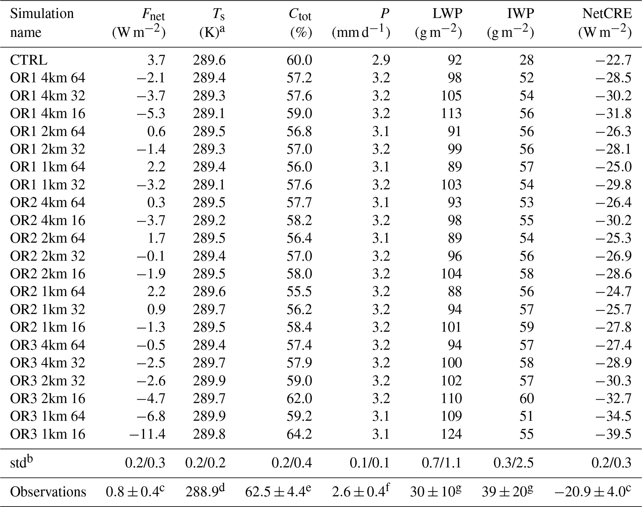
^a Model average surface temperature over land is represented by values of the lowermost model layer. ^b Standard deviations of two multi-year simulations each spanning 10 years. Configurations OR1 4km 64 and OR2 1km 16 have been utilised for these long runs. ^c CERES Energy Balanced and Filled (EBAF)-TOA edition 2.8 (Clouds and Earth's Radiant Energy System – Energy Balanced and Filled) – April 2000–March 2010; Wielicki et al. (1996) and Loeb et al. (2009). ^d NCEP/DOE2 reanalysis data provided by the NOAA/OAR/ESRL PSD, Boulder, CO, USA, from their website at https://www.esrl.noaa.gov/psd/ (last access: 15 March 2020) – January 1979–December 2010; Kanamitsu et al. (2002). ^e CERES ISCCP-D2LIKE-MERGED – edition 3A, NASA Langley Atmospheric Science Data Center DAAC; https://doi.org/10.5067/Aqua/CERES/ISCCP-D2LIKE-MERG00_L3.003A – April 2000–March 2010; Wong (2008). ^f Global Precipitation Climatology Project (GPCP) Climate Data Record (CDR), version 2.3 (monthly). National Centers for Environmental Information; DOI: https://doi.org/10.7289/V56971M6 – January 1981–December 2010; Adler et al. (2018). ^g CM SAF CLARA-A2 (the Satellite Application Facility on Climate Monitoring Cloud: albedo and surface radiation dataset from Advanced Very High Resolution Radiometer (AVHRR) data – second edition) – April 1986–March 2010; https://doi.org/10.5676/EUM_SAF_CM/CLARA_AVHRR/V002; Karlsson et al. (2017).

In order to classify these single-year averages, two additional multi-year simulations have been conducted using configurations OR1 4km 64 and OR2 1km 16. These simulations help to estimate the annual variability for SP-EMAC simulations. The associated standard deviations are given in Table 2.

Considering the radiative fluxes at TOA, almost all configurations of the superparameterisation lie within a range of ±4 W m⁻², reflecting an almost balanced radiation budget. Only two setups (OR3 1km 64 and OR3 1km 16) show a strong negative imbalance generated by too-reflective clouds. The energy deficit for these simulations can be explained by a large negative net cloud radiative effect dominated in the shortwave and an overestimation of LWP. Additionally, it should be mentioned that the high imbalance is only seen for the 3-D setups of SP-EMAC. Changing the size or number of cells in a three-dimensional CRM setup drastically changes the covered area of the superparameterisation. This modification (reduction in CRM area) seems to significantly influence the CRM properties to correctly simulate the mean effects of subgrid-scale processes within a GCM cell. A similar 3-D CRM configuration (in terms of CRM domain size) is applied in Parishani et al. (2017) with the exception of using a much higher horizontal (250 m) and vertical (down to 20 m) resolution. Focusing on shallow cumulus clouds, this work presents improved cloud cover profiles of boundary layer clouds but an enhanced shortwave cloud radiative effect, resulting in a strong global mean bright bias. The latter result is comparable to the imbalanced simulations mentioned above. An evident cause is the restricted CRM domain size that plays a crucial role for the development of deep convection and associated high clouds by cold pools and mesoscale organisation (Tompkins, 2001). Another possible feedback that could degrade global statistics, affecting large-scale dynamics for all OR3 simulations, is the momentum transport, which is different in comparison to the two-dimensional CRM setups. Nevertheless, these simulations (no. 20 and no. 21 in Table 1) are discarded from further analysis because the mean climate is highly deteriorated. Concerning the range of averaged surface temperature over land (neglecting the Arctic and Antarctica) values between 289 and 290 K mirror the variability of the SP-EMAC ensemble. All simulations including the control simulations depict a higher surface temperature compared to reanalysis data. The difference is partly due to the model output variable that presents the temperature of the lowermost model layer instead of using the 2 m temperature. The variability in mean surface temperature over land emphasises the influence on the planetary boundary layer due to a change in the hydrological cycle. Previous studies (Qin et al., 2018; Sun and Pritchard, 2018) have shown that land–atmosphere coupling is improved using a superparameterisation. Nevertheless, these results rely on one specific CRM setup. The 1 K variability in near-surface temperature suggests a non-negligible effect on the hydrological and thermal coupling due to different CRM configurations.

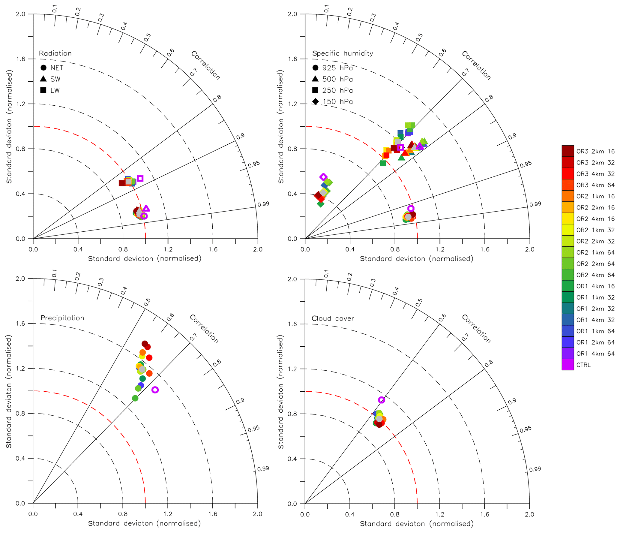
Figure 2 Taylor diagrams summarising radiative fluxes at TOA, specific humidity on selected pressure levels, precipitation and total cloud cover. Individual simulations are colour-coded, whereas grey markers represent the overall SP-EMAC ensemble. The control simulation is marked with open purple–white symbols. Observational data for radiation at TOA, total cloud cover and precipitation are the same as indicated in Table 2. For specific humidity, NCEP/DOE2 reanalysis data are used from January 1979 to December 2010 and evaluated only over continental points.

In contrast to T_s, the variability in mean global precipitation (P) is small. Almost all SP-EMAC configurations display similar global-averaged precipitation amounts. All superparameterised simulations show slightly overestimated precipitation rates in comparison with GPCP (Global Precipitation Climatology Project) data and their uncertainty. In a global context, the CRM configuration does not have an effect on annual mean precipitation, but significant differences occur spatially depending on the chosen setup (see Sect. 3.2). The total cloud cover for all superparameterised simulations is underestimated by 5 % with the current setup of SP-EMAC. Similar underestimations in cloud amount and overestimation in cloud optical depth (see Sect. 3.3) have been observed in past multiscale modelling framework (MMF) studies (Marchand and Ackerman, 2010; Parishani et al., 2017). However, a cloud coverage around 57 % still lies within the range (at the lower end) of current estimates of several GCMs participating in the Coupled Model Intercomparison Project phase 3 and phase 5 (CMIP3 and CMIP5; Probst et al., 2012; Calisto et al., 2014). Nevertheless, this deficit can be compensated by further tuning efforts, as it has been done for the control simulation, depicting a mean total cloud cover of 60 % (Mauritsen et al., 2012). Because deficiencies in cloud amounts are closely related to the liquid and ice water path, even higher differences are expected to arise. Best estimates for globally averaged LWP (IWP) based on different observational datasets expose a highly uncertain range between 30 and 50 g m⁻² (25–70 g m⁻²), with an upper limit of 100 g m⁻² (140 g m⁻²) (Jiang et al., 2012). These differences are due to different satellite sensor sensitivities, attenuation limits, retrieval errors and algorithmic assumptions, therefore showing no clear consensus throughout the literature (O’Dell et al., 2008; Stubenrauch et al., 2013). Comparing AVHRR (Advanced Very High Resolution Radiometer) satellite data with model results displays high discrepancies in liquid and ice partitioning. Similar to the control run, all SP-EMAC configurations show a comparable mean LWP around 90 to 110 g m⁻². These high amounts of liquid water in the atmosphere seem to extremely overestimate the underlying observations of CM SAF (the Satellite Application Facility on Climate Monitoring) but are on the upper range of current LWP estimates and GCM simulations (Lauer and Hamilton, 2013). Previous studies have shown relatively high amounts of LWP and IWP for SP-CAM as well (Wyant et al., 2006b; Parishani et al., 2018). The most likely reasons for very high IWP values (and LWP values) are due to parameter settings within the CRM's cloud microphysics. Because, as opposed to the control simulation, the new model was not tuned to a proper extent, setting the parameters within the cloud microphysics (i.e. autoconversion thresholds of ice/liquid, terminal fall velocity or the temperature bounds of ice–liquid partitioning) could easily lead to lower (more realistic) values (see Parishani et al., 2018, Table 2). Because we have used the same parameters as noted in Table 1 (simulation SPCTRL) of Parishani et al. (2018), the IWP/LWP are on the upper range of observations. Nevertheless, tuning of several parameters could lead to unintended effects because of nonlinear interactions, thereby influencing other quantities like cloud cover or cloud radiative effect. The physical processes during model integration of rationing cloud water into its liquid and ice phase is a compensating effect on total cloud cover and radiation. In addition to LWP/IWP estimates, precipitable water (i.e. integrated water vapour) displays a range between 24.9 and 25.9 mm for all SP-EMAC runs (CTRL: 24.9 mm), whereas most simulations lie within 24.9 and 25.6 mm. These values lie within observational constraints and past model studies (Demory et al., 2014).

One last major aspect to consider is the net radiative effect of clouds that is affected by the total cloud cover as well as their optical thickness and vertical extent. Absorption and reflectance of solar and terrestrial radiation is influenced by the presence of clouds and the total net cloud radiative effect (at TOA) can be quantified as the sum of its shortwave and longwave components:

$$\begin{array}{ll}{\displaystyle }\text{NetCRE}& {\displaystyle }={\text{CRE}}_{\text{SW}}+{\text{CRE}}_{\text{LW}}\\ {\displaystyle }{\text{CRE}}_{\text{SW}}& {\displaystyle }=({\text{SW}}^{\downarrow }-{\text{SW}}_{\text{all}}^{\uparrow })-({\text{SW}}^{\downarrow }-{\text{SW}}_{\text{clear}}^{\uparrow })\\ {\displaystyle }& {\displaystyle }={\text{SW}}_{\text{clear}}^{\uparrow }-{\text{SW}}_{\text{all}}^{\uparrow }\\ {\displaystyle }{\text{CRE}}_{\text{LW}}& {\displaystyle }=({\text{LW}}_{\text{all}}^{\downarrow }-{\text{LW}}_{\text{all}}^{\uparrow })-({\text{LW}}_{\text{clear}}^{\downarrow }-{\text{LW}}_{\text{clear}}^{\uparrow })\\ {\displaystyle }& {\displaystyle }={\text{LW}}_{\text{clear}}^{\uparrow }-{\text{LW}}_{\text{all}}^{\uparrow },\end{array}$$

where ${\text{SW}}_{\text{clear}}^{\uparrow }$ and ${\text{SW}}_{\text{all}}^{\uparrow }$ describe the clear-sky and all-sky reflected shortwave radiation at TOA and ${\text{LW}}_{\text{clear}}^{\uparrow }$ and ${\text{LW}}_{\text{all}}^{\uparrow }$ represent clear-sky and all-sky outgoing longwave radiation (OLR) at TOA.
The NetCRE is negative describing an overall cooling effect of clouds on the atmosphere. Concerning all simulations, CTRL shows with −22.7 W m⁻² a net cloud radiative effect closest to the observed value of −20.9 W m⁻² (cf. Table 2 NetCRE observed by CERES Energy Balanced and Filled (EBAF)-TOA edition 2.8). The SP-EMAC simulations cover a range between −24.7 and −32.7 W m⁻², which seems even more surprising because total cloud cover is slightly reduced in all superparameterised simulations.

This change would usually lead to a smaller NetCRE, which is not the case. Therefore, optical properties of clouds must have substantially been changed in all SP-EMAC runs, indicating an increased reflection of radiation by clouds. This is evaluated in more detail in Sect. 3.3. All in all, without tuning of SP-EMAC, almost all CRM configurations of SP-EMAC show mean climate characteristics equivalent to the control simulation and lie within a comparable range to observational estimates.

Apart from the analysis of averaged global fields, Fig. 2 displays normalised Taylor diagrams (Taylor, 2001) for four different quantities. These types of diagrams condense various aspects of multidimensional variables in comparison to observational data in one plot. The similarity of simulated and observed patterns is quantified in terms of correlation, standard deviation and centred root mean square error (RMSE). In total, the correlation (R) given by the azimuthal angle, the standard deviation (σ), which is proportional to the radial distance from the origin, and the RMSE corresponding to the distance from the observational point (which is aligned at a unit distance from the origin along the x axis) quantify the degree of agreement between modelled and observed fields. The correlation coefficient includes spatial as well as temporal correlation for all variables based upon monthly averages reflecting the pattern concurrence in time and space. The Taylor diagram characterises the similarity based upon statistical relationships between modelled and observed fields. In order to compare these fields, all observations are remapped onto the applied model resolution (T42 ≈ 2.8^∘ at the Equator).

All simulations show shortwave and net radiative fluxes at TOA that are in close agreement to observed fields (R≈0.98). Further focusing on the shortwave and net radiative flux, no significant improvement of SP-EMAC in comparison with CTRL can be deduced from the Taylor diagram but an overall very similar global skill is achieved. Concerning longwave TOA radiative fluxes, the correlation is slightly reduced (R≈0.86), and all SP-EMAC runs demonstrate a better variance than CTRL.

Significantly improved performance in terms of correlation and variability is also visible for total cloud cover, reducing the centred RMSE by 10 %. The latter is a direct result of an improved representation in the Northern Hemisphere total cloud cover (not shown), whereas tropical and large ocean fractions show an underestimation for the superparameterised simulations. The improvements in radiation and total cloud coverage suggest a better representation of cloud–radiation processes caused by the ability to include subgrid-scale cloud dynamics.

When comparing the continental humidity distribution for four atmospheric levels, interesting features appear. In order to compare all simulations, reanalysis of NCEP has been used as quasi-observations on a global scale. Lower-level specific humidity at 925 hPa shows a high correlation (R≥0.95) and a comparable standard deviation for many SP-EMAC runs against reanalysis data. All superparameterised model runs show a higher correlation than CTRL and are bundled together for the lowermost tropospheric level without an apparent spread. This behaviour reflects the importance of interactions between boundary layer processes and precipitating fields. An even bigger spread is visible for mid-level and upper troposphere humidity at 500 and 250 hPa. Two features are prevailing: a decrease in correlation with increasing altitude and a higher variance for almost all simulations. The overestimated variability of specific humidity is mainly a cause of too much water vapour transport over tropical continents and not enough over tropical oceans. The decrease in the correlation coefficient expresses the difficulty to simulate the appropriate water vapour transport for higher atmospheric levels, especially in the intertropical convergence zone (ITCZ). Moreover, it is obvious that different SP-EMAC configurations have a strong impact on the upper tropospheric moisture budget at 250 hPa. This is a consequence of contrasting CRM resolved strength of vertical winds. When evaluating specific humidity distribution at the tropical tropopause level near 150 hPa, almost no correlation remains and variability in these heights is strongly underestimated. This uncorrelated relationship is negatively influenced by an almost unresolved stratospheric circulation because of the sparse vertical resolution in these heights. This is an indication of almost no water vapour transport via the Brewer–Dobson circulation from the tropics to the poles.

The representation of precipitation and its spatial and temporal distribution is slightly worse compared to the CTRL simulation, with correlations less than 0.7. Furthermore, the configuration of SP-EMAC strongly modifies the distribution of rainfall within the CRM columns. A much bigger spread is visible in the Taylor diagram for precipitation comparing individual SP-EMAC runs. This pinpoints the importance of the CRM configuration onto the global precipitation distribution and will be explored in more detail, focusing on regional differences in the next section.

Recapitulating the evaluation of global SP-EMAC fields, several Taylor diagrams show a similar spatial and temporal correlation compared to the control simulation with parameterised convection. A slight improvement in the longwave radiative flux and total cloud cover distribution is seen in the Taylor diagrams.

Figure 3 Zonal-averaged simulated precipitation compared to GPCP data.

The representation of precipitating fields is slightly deteriorated. Accompanying tuning efforts for SP-EMAC could easily outperform the control simulation and thereby show the advantage of resolving small-scales features and their impact onto global metrics.

3.2 Influence on regional aspects

The introduction of a superparameterisation resolving cloud dynamics in a GCM explicitly implies changes of local phenomena like precipitation, cloud regimes or boundary layer characteristics.

Figure 4 Differences in precipitation of the SP-EMAC ensemble (a) and CTRL (b) in contrast to global observations (GPCP). Coloured areas show only regions with significant differences in precipitation (analysed with t tests on a significance level of 90 %).

This section evaluates regional patterns of precipitation and cloud radiative effects of SP-EMAC. In addition to that, the diurnal cycle of tropical precipitation is diagnosed as well as probability density functions (PDFs) for specified regions.

As a first step, significantly different precipitating regions for all simulations are identified and compared to observations. Moreover, facing current deficiencies of GCMs, two specified regions are taken into account to analyse simulated precipitation features: maritime tropics (in particular, the warm pool region) and the southern midlatitudes. In previous literature, it has been shown that the maritime continent depicts too much precipitation for all CMIP5 models consistently (Flato et al., 2013). In addition to that, simulating the Asian summer monsoon tends to overestimate rainfall amounts by a too-strong convection–wind–evaporation feedback using a convection parameterisation or a superparameterisation (Luo and Stephens, 2006). Complementarily, an overestimation in oceanic precipitation frequency is simulated over the Southern Hemisphere, indicating too much drizzle (Stephens et al., 2010). Although a new study suggested that these biases originate from processes other than convection, a reduction of these errors is clearly accomplished by using convection parameterisations (Maher et al., 2018). The comparison of SP-EMAC with observations and a parameterised control simulation will reveal the importance of resolving subgrid-scale dynamics in a superparameterised GCM for these regional improvements.

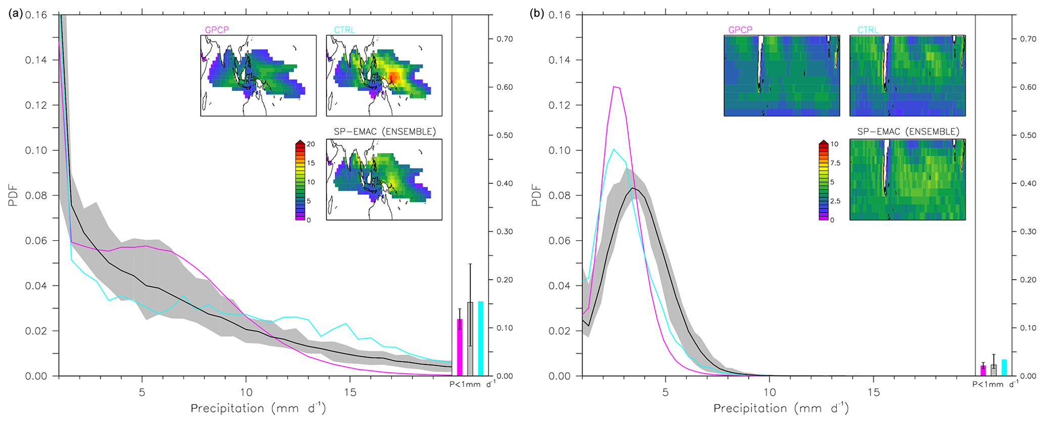
Figure 5 PDFs of monthly precipitation rates for the warm pool region (a) and Southern Ocean midlatitudes (b) compared to 30 years of GPCP data (same as in Table 2). Inserted maps show yearly averaged rates in mm d⁻¹ for the specified geographical regions as pointed out in the text. Line colours correspond to the colours above the inserted panels. On the right-hand side of each figure, the fraction of non-precipitating cells (below 1 mm d⁻¹) is displayed, including the interannual variability for the GPCP data and the variability induced by different SP-EMAC configurations (uncertainty bars). Note that the x axis begins at 1 mm d⁻¹.

Figure 3 shows zonal-averaged precipitation rates for SP-EMAC, CTRL and GPCP data. In correspondence, Fig. 4 highlights regions with significant differences in annual mean precipitation compared to observations. These regions have been identified by a couple of t tests on a significance level of 90 %. For the control simulation, a single t test has been carried out to emphasise important areas. Considering the analysis for SP-EMAC, regions are highlighted when more than half of all superparameterised simulations show a significant difference between observed and modelled fields. The control simulation is in close agreement to the GPCP observations with the exception of enhanced tropical precipitation, which is well represented by the superparameterisation. Contrary to this, an overestimation in the northern and southern midlatitudes is visible for SP-EMAC, independent of the chosen CRM configuration. This finding is in agreement with the study of Marchand et al. (2009), showing an overestimation of low-level hydrometeors in midlatitude storm tracks using the same superparameterisation within SP-CAM (Superparameterised Community Atmosphere Model). An improvement is given by Kooperman et al. (2016), showing no systematic biases within the midlatitudes using a two-moment microphysical scheme linked to aerosol processes (Wang et al., 2011a). Regardless of these studies, SP-EMAC sensitivity runs suggest that formation of precipitation including the ice phase (or mixed phase) is substantially better simulated than rainfall in almost pure liquid clouds, which is often the case for maritime precipitation in the southern midlatitudes (Matsui et al., 2016). Nevertheless, a high sensitivity in precipitation is simulated within the ITCZ and the northern and southern midlatitudes depending on the CRM configuration. Analysing this in more detail, it emerges that the contribution of this variability is mostly generated above the oceans and coastal regions (not shown). That implies that simulated precipitation rates are sensitive to land–ocean contrasts.

Focusing on two specific regions, Fig. 5 displays probability density functions of monthly precipitation rates for the warm pool region and the Southern Ocean midlatitudes. The former is defined as an area where sea surface temperatures exceed 297 K and strong convective systems develop, whereas the latter defines only oceanic regions in the Southern Hemisphere between 36 and 64^∘, characteristically associated with marine boundary layer clouds (Mace, 2010; Haynes et al., 2011). Embedded maps present the spatial distribution for the chosen region as yearly averaged precipitation rates. In addition to that, the non-precipitating fraction (below 1 mm d⁻¹) is shown as bars, including the variability of SP-EMAC, induced when choosing different configurations and the interannual variability of the observational data. Based on the overall improvement for SP-EMAC to simulate precipitation in the warm pool region, the PDF shows important characteristics that are to some extent reproduced by the superparameterisation. The most distinct feature for the maritime continent PDF is the high variability for the SP-EMAC simulations covering almost the entire range of observed probabilities. Compared to the control simulation, it is most obvious that high precipitation rates (above 10 mm d⁻¹) are better represented by the CRM. Precipitation rates between 3 and 10 mm d⁻¹ are underestimated by almost all simulations. Depending on the chosen configuration, it can be concluded that the OR1 4km 64, OR1 2km 64, OR2 4km 64 and OR2 2km 64 configurations produce the best estimate of precipitation in the warm pool region (not shown). Each of these simulations shows enhanced precipitation probabilities between 5 and 10 mm d⁻¹ and produces the lowest probabilities for high precipitation rates in agreement with the GPCP observations (not shown). Comparing the spatial distributions, a single maximum precipitation spot is visible in the western Pacific when using the convection parameterisation. This is not as prominent for the SP-EMAC simulations displaying a more widespread distribution. At last, non-precipitation probabilities (comparing boxes on the right side of the plot) are in close agreement with the GPCP data but expose a huge variability for SP-EMAC, reflecting the strong dependence on the chosen configuration.

Figure 6 Comparison of diurnal tropical precipitation (30^∘ around the Equator) for land and ocean with 3-hourly Tropical Rainfall Measuring Mission (TRMM) data^∗ between 1998 and 2010 for the month of July. The observational standard deviation is shown by error bars indicating interannual variability in the diurnal cycle. The grey area covers the variability of all SP-EMAC configurations. ^∗ TRMM (2011), TRMM (TMPA) rainfall estimate, L3, 3 h, $\mathrm{0.25}{}^{\circ }\times \mathrm{0.25}{}^{\circ }$, V7, Greenbelt, MD, Goddard Earth Sciences Data and Information Services Center (GES DISC); https://doi.org/10.5067/TRMM/TMPA/3H/7; Huffman et al. (2007).

The comparison of precipitation rates in the Southern Hemisphere midlatitudes reveals two systematic problems of SP-EMAC: an underestimation of lower precipitation rates (between 1 to 5 mm d⁻¹) and a shift in peak precipitation rate from the observed value of 2.5 mm d⁻¹ to almost 4 mm d⁻¹, explaining the overestimation in Fig. 3. This feature is significant for all superparameterised simulations independent of the chosen CRM configuration. Furthermore, the comparison of almost non-precipitating grid cells reveals a similar amount of dry days in comparison with the control simulation. This finding is in agreement with other models showing a similar behaviour between parameterised and superparameterised simulations (see Kooperman et al., 2016, Supplement S2). All in all, the control simulation can reproduce the peak precipitation, whereas it is skewed to larger values (above 4 mm d⁻¹). Pointing out the differences in the microphysics, one has to consider the different autoconversion rates used within the CRM cells and within the cloud scheme of the control run. The superparameterisation uses a simple fixed conversion rate (see Khairoutdinov and Randall, 2003, Appendix D), whereas the cloud scheme uses the formulation of Beheng (1994). Focusing on this aspect, Suzuki et al. (2015) has shown that the distribution of precipitation categories (non-precipitating, drizzle, rain) is dependent on its expression, thereby influencing the precipitation rate. Future studies with SP-EMAC should investigate the onset of precipitation for maritime clouds in more detail or should consider using a two-moment microphysical scheme and its coupling to an aerosol submodel.

Apart from the distribution of precipitation, a known problem of GCMs is the incorrect representation of the diurnal cycle in precipitation within the tropics (Collier and Bowman, 2004; Guichard et al., 2004; Dai, 2006). Improvements have been suggested by Bechtold et al. (2004) for convection parameterisations based on their entrainment rates. Additionally, superparameterised GCMs have been studied and show progress in representing the diurnal cycle of precipitation and its contrast between ocean and land (Khairoutdinov et al., 2005; Zhang et al., 2008; Pritchard and Somerville, 2009a, b; Tao et al., 2009). In order to analyse this process, the output has been increased to produce precipitation rates on a hourly basis for an entire month (July). Instead of using the full SP-EMAC ensemble, only a subset of superparameterised simulations with an annual precipitation below 3 mm d⁻¹ has been chosen. These simulations have been selected because they have the smallest difference in comparison to observational data (compare with Table 2). The hourly output has been compared to multi-monthly July averages of Tropical Rainfall Measuring Mission (TRMM) 3B42 v7 data between 1998 and 2010. Figure 6 displays the averaged diurnal precipitation transformed to local solar time (LT) for continental and oceanic grid points between 30^∘ latitudes around the Equator. Investigating the diurnal precipitation over land, observational evidence exposes a peak around 17:00 LT and an onset in precipitation around 09:00 LT. Previous studies of different TRMM products (3B42 and 3G68) have revealed a time lag, which may be related to infrared precipitation estimates (Kikuchi and Wang, 2008). It had been stated that the maximum peak in TRMM_3G68 is more reliable, occurring at 15:00 LT. Therefore, TRMM product 3B42 shows a lag of approximately 3 h opposed to 3G68, which need to be taken into account for this study (Sato et al., 2009). This time lag seems to be valid for the maximum peak but not the onset in precipitation (Sato et al., 2009). The control simulation does not reproduce any of these timings, confirming the difficulty of GCMs including convection parameterisations to correctly simulate the diurnal cycle. The onset and peak of precipitation are around 4 h too early and the amplitude is overestimated. Many aspects of this evolution can be attributed to diminishing CIN (convective inhibition) during sunrise and increasing CAPE (convective available potential energy) during the day that are the basis of triggering and sustaining the convection parameterisation. The shift of a too-early precipitation onset is substantially improved using any kind of SP-EMAC simulation. Independent of the CRM configuration, the timing of the onset of precipitation is almost perfectly reflected in comparison to 12-year-averaged TRMM data for the month of July (see Fig. 6). This indicates that cloud evolution is not only coupled to the diurnal solar insolation but follows planetary boundary layer (PBL) evolution. In contrast, diurnal peak precipitation is completely dependent on the CRM configuration for SP-EMAC indicating values between 2.5 and 3.75 mm d⁻¹ and peak time spreading from 12:00 LT (OR1 1km 16) to 17:00 LT (OR2 4km 64). Taking into account that the observational product has a lag of 3 h, some SP-EMAC configuration provides good estimates in the timing of maximum precipitation. Furthermore, the decline in precipitation after peaking is too strong, resulting in a secondary maximum during the night (between 02:00 and 05:00 LT). This secondary peak is partly visible for the TRMM data but only for spring and autumn seasons (Yang and Smith, 2006). Even if the diurnal cycle is not captured very well, it has almost no influence on the global mean precipitation rate. One significant highlight corresponds to the different diurnal amplitudes, which increase with increasing number of CRM cells, whereas single simulations with 32 or 16 cells exhibit a small or almost no diurnal cycle in precipitation.

The diurnal cycle over tropical oceans is displayed on the right side in Fig. 6. The observed diurnal cycle presents a peak in precipitation around 06:00 LT and a clear minimum in the evening hours (21:00 LT). A saddle point (secondary maximum) can be identified around 14:00 LT. The primary mechanisms to explain this cycle are “static radiation–convection” and “dynamic radiation–convection”, which describe the process of radiative cooling while increasing thermodynamic instability enhancing nighttime precipitation or suppressing daytime rainfall through decreased convergence into the convective region. A more detailed description and further mechanisms are given in Yang and Smith (2006).

The control simulation shows an overall overestimation of oceanic precipitation rates by 0.5 mm d⁻¹ but a similar timing in peak precipitation. The simulated decline in oceanic rainfall is too steep, resulting in too-early minimum precipitation rate around 15:00 LT and an increase directly afterwards. In contrast, nearly all SP-EMAC runs simulate a consistent decline as CTRL after peaking precipitation between 04:00 and 06:00 LT but remain almost constant until 21:00 LT. The spread in oceanic precipitation rates of the SP-EMAC ensemble is slightly lower (0.75 mm d⁻¹) compared to the diurnal cycle over land (1.25 mm d⁻¹). Analogous to the diurnal cycle over land, it emerges that the amplitude of precipitation rates increases with an increasing number of CRM cells. Especially two specific configurations (OR1 2km 64 and OR2 4mk 64) are in very good agreement with TRMM data. Nevertheless, all simulations miss the representation of a secondary maximum around 14:00 LT. This effect could be due to neglected diurnal variations in prescribed SSTs, thereby restraining ocean surface heating (Sui et al., 1997, 1998). Further investigations of 2-D cloud-resolving model simulations with diurnally varying SSTs exhibit an increase in afternoon rain rates suggesting influences of ocean heating in atmospheric moistening and drying throughout the day (Cui and Li, 2009).

To complete the regional analysis of SP-EMAC, cloud radiative effects at the top of the atmosphere are investigated.

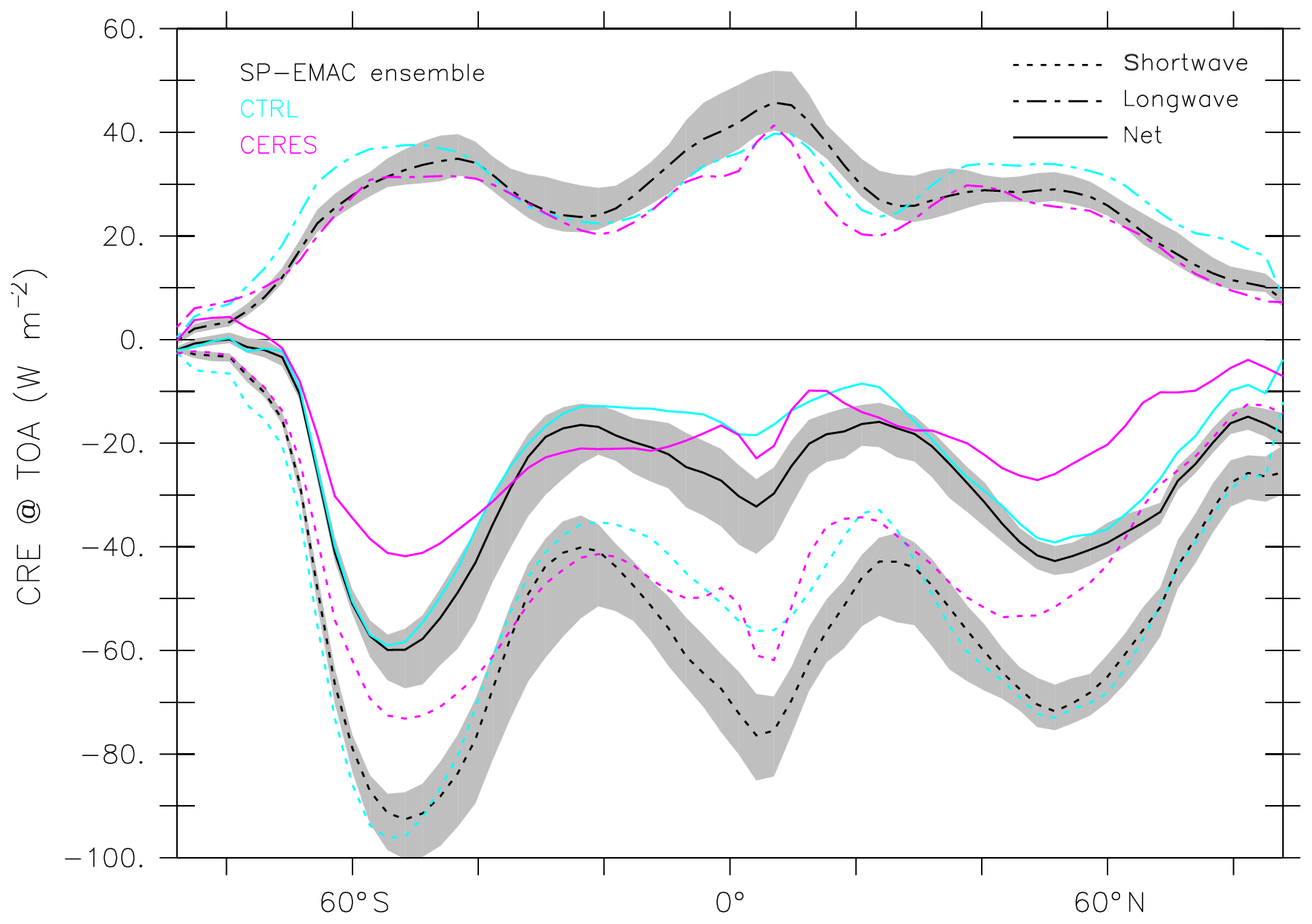
Figure 7 Zonal-averaged simulated top-of-atmosphere cloud radiative effects (CREs) compared to CERES EBAF-TOA data (2000–2010).

Overall, 10 years of satellite data of CERES are used for comparison (see Table 2). CRE is divided into its longwave and shortwave components to distinguish different radiative effects. Zonal averages of cloud radiative effects are shown in Fig. 7.

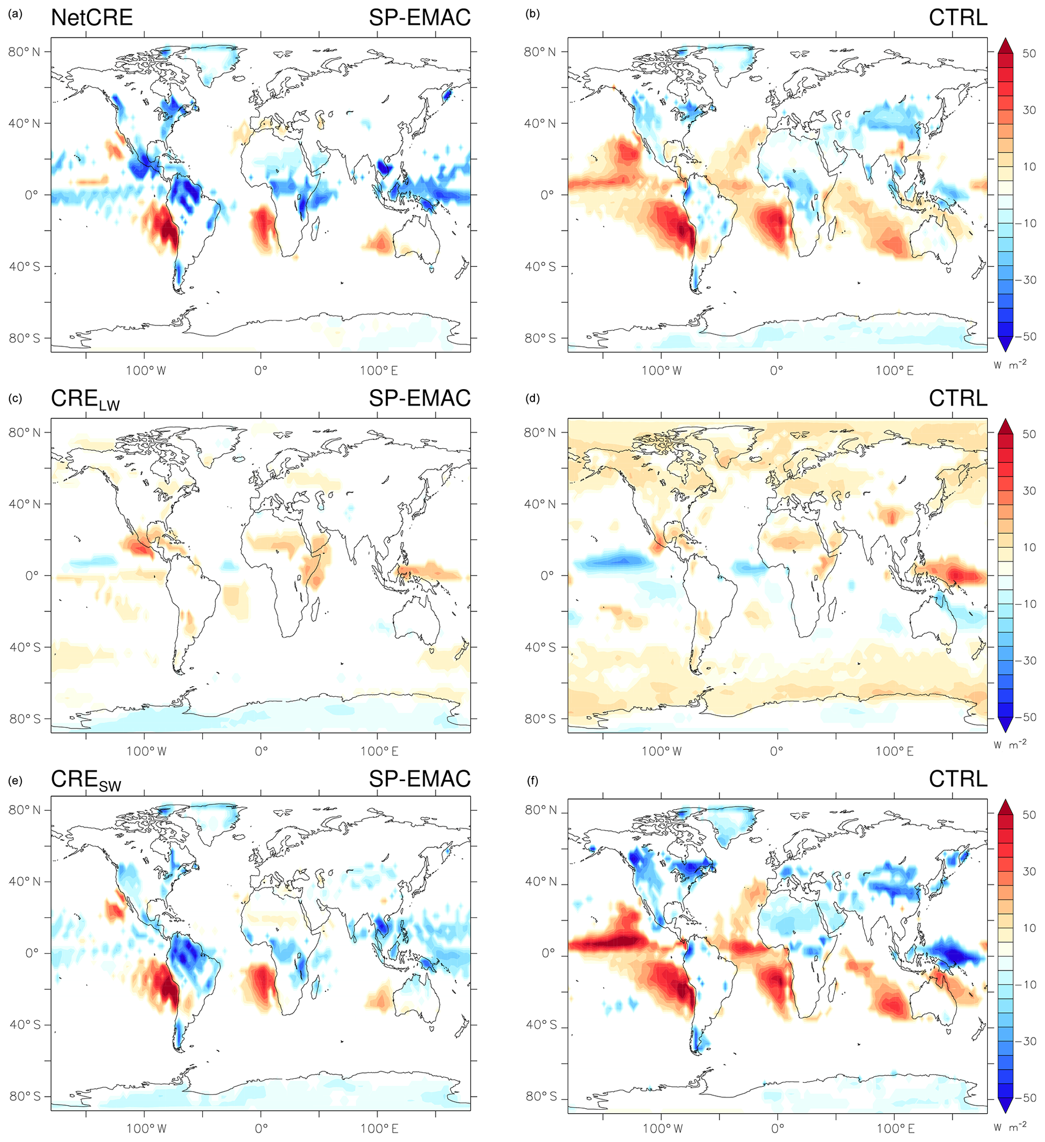
Figure 8 Differences in simulated and observed cloud radiative effects at TOA: net (a, b), longwave (c, d) and shortwave (e, f). Results for SP-EMAC ensemble (a, c, e) and CTRL (b, d, f) are shown compared to global observations (CERES). Coloured areas show only regions with significant differences in cloud radiative effects (analysed with t tests on a significance level of 90 %).

Instead of displaying all individual SP-EMAC simulations, the ensemble mean (black lines) and spread (grey area) are shown. The distribution of NetCRE shows high discrepancies in the midlatitudes. The primary cause of this difference is induced by the shortwave component of the CRE revealing the representation of too-reflective clouds in all simulations for this region. Moreover, seasonal variation for CRE_SW is enhanced in all SP-EMAC simulations as well as in the control run. Smaller deviations for NetCRE are visible in the ITCZ for SP-EMAC compensated by even larger differences for the individual components CRE_SW and CRE_LW. Comparing CTRL and SP-EMAC in a comprehensive sense, it emerges that overall CTRL represents the zonal NetCRE distribution slightly better especially in the tropics. This is sometimes due to compensating errors. On a closer look, many SP-EMAC configurations improve the longwave and shortwave components in the midlatitudes. Nevertheless, dependent on the CRM configuration, there exist large differences even in the zonal-mean distribution. To identify regions with significant differences, Fig. 8 shows absolute differences of NetCRE, CRE_SW and CRE_LW. Similar t tests as for Fig. 4 have been performed to obtain important areas that deviate from CERES observations. Thereby, non-significant differences are shown in white. Blue areas indicate regions where cloud radiative effects are stronger (higher cooling), whereas red areas specify less cooling or even a warming effect of clouds. Comparing the differences in NetCRE maps in Fig. 8, it is apparent that CTRL shows larger areas of significant differences especially a positive bias over the oceans. The underestimation of cloud radiative effects for CTRL over the oceans is because of a much higher shortwave component in these regions, marking a reduced amount in low cloud cover or less reflective clouds in the areas of stratocumulus decks. Using a superparameterisation in EMAC results in smaller discrepancies for all CRE components. In particular, the formerly mentioned regions demonstrate a better representation of radiative effects of low clouds. However, a significant reduction of about 10 to 20 W m⁻² is visible for the western Pacific region in many SP-EMAC simulations. When evaluating the longwave and shortwave components in these region, it became apparent that deep convective clouds have an increased optical depth for many CRM configurations and concurrently a higher liquid and ice water content than the control simulation (not shown). Further important differences are visible for CRE_LW in the control simulation.

A stronger warming over the complete Southern Ocean and the Arctic region is apparent as a result of a too-high liquid water path in these regions. Lastly, comparing all maps from top to bottom in Fig. 8, it is possible to easily identify regions that show almost no significant difference in NetCRE because of compensating errors in the longwave and shortwave parts. Affected areas are central Africa, Central America and the Caribbean Sea for SP-EMAC and the Sahara, Greenland, North America, the Arctic and the Southern Ocean for CTRL. Thereby, it is evident that NetCRE should not be used as a single metric to evaluate cloud radiative effects and the performance of a GCM. All in all, CRE is influenced by multiple factors: insolation, cloud amount, cloud type and surface properties (albedo). Only cloud amount and cloud-type changes are relevant for explaining differences between SP-EMAC and CTRL (excluding glaciers and snow-covered areas that increase surface albedo). Even if SP-EMAC seems to reduce CRE errors, different configurations show significant different results. Future studies with SP-EMAC should always look at the different cloud radiative effects to avoid misinterpretations of model results. This is necessary because not all SP-EMAC configurations are equally appropriate to use. This addresses the need for a tuning activity for SP-EMAC in the near future.

3.3 Issues due to CRM's configuration

The global evaluation of SP-EMAC in Sect. 3.1 has revealed some major influences of the CRM configuration onto the mean climate state. This is in particular very important concerning regional aspects of clouds and precipitation.

Based upon the global mean Taylor diagrams in Fig. 2, no clear separation of several SP-EMAC simulations is noticeable. Tracking down other differences that indicate surface temperatures and precipitation rates among SP-EMAC simulations, the distribution of surface heat fluxes is analysed. Figure 9 shows the Taylor diagram of sensible and latent heat flux over land. The fluxes are compared to NCEP reanalysis data (compare with Table 2) between 1979 and 2010. Evaluating the Taylor diagram, it is clearly visible that heat fluxes are well reproduced, and all simulations are bulked together. This clustering suggests that boundary fluxes are hardly affected, even if the variability in mean global lowermost model temperature shows a not negligible range of 1 K. The analysis of heat fluxes clearly shows that the configuration (changing the size, number and orientation of the CRM) does not impact lower tropospheric properties. This independence of boundary layer fluxes on the SP-EMAC configuration is an addition to the analysis of Sun and Pritchard (2018) and Qin et al. (2018) providing a better or equal representation of the thermal and hydrologic coupling. One further modification to expand this framework could be the consideration of the large-scale directional wind speed within the CRM. All two-dimensional setups use either the zonal (OR1 cases) or meridional wind component (OR2 cases). Allowing the 2-D CRM to vary with time (Grabowski, 2004a; Cheng and Xu, 2014; Jung and Arakawa, 2016) could have an impact on the boundary layer turbulence and hence modify the boundary layer fluxes.

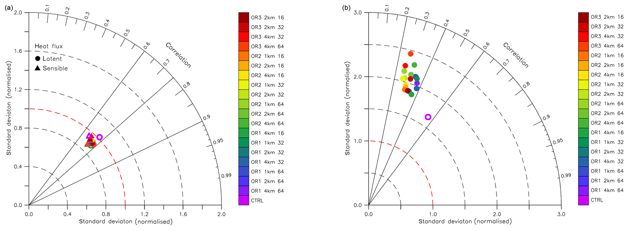
Figure 9 Global Taylor diagrams of sensible and latent heat fluxes (a) and cloud optical thickness (b) over land points only. The control simulation is marked with open purple–white symbols. For comparison purposes, reanalysis data of NCEP are taken to compare all simulations with respect to heat fluxes, and MODIS retrievals provide estimates of cloud optical properties.

Instead of analysing indirect effects like surface fluxes, global mean precipitation shows a more widely dispersed result in Fig. 2. In order to look at rather explicit effects of the CRM on cloud properties, it is therefore straightforward to observe cloud-related variables. Therefore, cloud optical thickness (COT) for continental clouds is examined using satellite data from the Moderate Resolution Imaging Spectroradiometer (MODIS) collection 5.1. Observations between 2003 and 2015 from the combined Terra and Aqua satellites are remapped onto the coarse GCM grid and used for comparison purposes. Figure 9 shows the Taylor diagram of cloud optical thickness. As opposed to the Taylor diagram of heat fluxes, a more widespread depiction of the SP-EMAC ensemble is apparent for COT. It clearly shows that cloud optical properties significantly changed within SP-EMAC in comparison to the control simulation. Generally speaking, all SP-EMAC simulations display a similar distribution as CTRL in the midlatitudes, whereas tropical cloud thicknesses over land are overestimated (not shown). This increase in COT partly explains the stronger cloud radiative effects for all SP-EMAC runs, compensating the overall reduced simulated total cloud cover. However, the comparison with MODIS data shows a strongly reduced correlation. A completely fair comparison with MODIS would imply the usage of the Cloud Feedback Model Intercomparison Project (CFMIP) Observational Simulator Package (COSP; (Bodas-Salcedo et al., 2011; Swales et al., 2018)). In addition to that, the neglect of subgrid-scale cloud variability is an important aspect to consider using the simulator (Song et al., 2018). Therefore, this comparison should be treated as a proxy to display the robust differences between SP-EMAC and CTRL including an observational reference for COT.

Although the representation of cloud optical thickness shows a larger spread within the SP-EMAC ensemble, it is not straightforward to identify CRM characteristics regulating the behaviour of the model. For this purpose, sub-ensembles are constructed to represent distinguishable results based upon the sub-ensemble typical feature. All 19 SP-EMAC simulations are described by three configurational aspects (differentiated by three different states; see Table 1). These aspects are used to create nine sub-ensembles consisting of the same state of the configurational assignment, i.e.

• OR1 consists of all simulations including the east–west orientation (simulation nos. 1 to 7 in Table 1).

• OR2 includes sim. nos. 8 to 15 (i.e. north–south-oriented CRM).

• OR3 covers sim. nos. 16 to 19 (only full 3-D CRM setups).

• 1km represents all simulations with a CRM grid size of 1 km (sim. nos. 6, 7, 13, 14 and 15).

• 2km represents sim. nos. 4, 5, 10, 11, 12, 18 and 19.

• 4km represents sim. nos. 1, 2, 3, 8, 9, 16 and 17.

• n16 describes all simulations with 16 CRM cells (sim. nos. 3, 9, 12, 15 and 19).

• n32 describes sim. nos. 2, 5, 7, 11, 14, 17 and 18.

• n64 describes sim. nos. 1, 4, 6, 8, 10, 13 and 16.

The aforementioned sub-ensembles are compared to the full SP-EMAC ensemble in order to distinguish effects that result from a specific configuration. Because cloud-related properties experience larger impacts due to a different configuration, full atmosphere cloud amounts are examined in Fig. 10.

Figure 10 (a, b) Averaged zonal cloud amount for the SP-EMAC ensemble and the control simulation. The black line marks the tropopause height. (c, k) Cloud amount differences of several SP-EMAC sub-ensembles in comparison to the SP-EMAC ensemble (top-right panel). The sub-ensembles are characterised by a CRM configuration feature; i.e. (c, d, e) OR1 consists of all simulations including the east–west orientation (the number of ensemble members is given in parentheses); OR2 consists of a sub-ensemble for north–south-oriented CRM cells; OR3 consists of a sub-ensemble of full 3-D CRM configurations; (f, g, h) 1 km/2 km/4 km consist of SP-EMAC simulations with CRM grid sizes of 1, 2 or 4 km; (i, j, k) n16/n32/n64 consist of SP-EMAC simulations including a total number of 16, 32 or 64 CRM cells.

Annual averages of zonal-mean cloud amounts for CTRL and the full SP-EMAC ensemble are displayed in the top row as a reference. SP-EMAC simulates lower cloud top heights than the control simulation and more pronounced convective cloud coverage within the ITCZ. Increased coverage of boundary layer clouds in the southern midlatitudes is visible. Despite the fact that major differences between the control simulation and SP-EMAC occur, sub-ensembles are analysed and compared to the full SP-EMAC ensemble. Absolute differences are displayed in Fig. 10, highlighting higher cloud amounts than in the reference in red colours. The partitioning of all SP-EMAC simulations into separate sub-ensembles leads to an easy identification of significant cloud amount changes due to different CRM configurations. Sub-ensembles of OR2, 2 km, 4 km and n32 show only minor differences in comparison to the full SP-EMAC ensemble. Regarding the orientation, cloud amounts show a slight increase in the midlatitudes for the zonal (OR1) CRM orientation, whereas the full three-dimensional orientation imprints a significant decrease for cloud amounts above 900 hPa. Additionally, an increase of boundary layer clouds in the Southern Hemisphere midlatitudes of OR3 exposes an effect of the lower tropospheric winds on cloud amount. Regarding the CRM grid size, it is clearly evident that a higher CRM resolution increases the amount of boundary layer clouds (see 1 km sub-ensemble in Fig. 10), which confirms the sensitivity study of Marchand and Ackerman (2010). Furthermore, a significant decrease in cloud amount is simulated for a smaller number of CRM cells (see sub-ensemble n16). Including the overall underestimation of total cloud cover for all SP-EMAC simulations, it appears that a minimum amount of 32 CRM cells is needed to provide a correct representation of cloud development within a GCM grid cell.

Similarities of sub-ensembles OR1 and n64 as well as OR3 and n16 are visible. These coincidences are due to individual SP-EMAC simulations, which demonstrate prominent features in cloud amount changes. For example, an increase in boundary layer clouds is seen for OR1 4km 64, OR1 2km 64 and OR1 1km 64 (not shown), which are within both sub-ensembles of OR1 and n64. Likewise, OR3 2km 16 and OR3 1km 16 show a decrease in boundary layer clouds, resulting in a similar appearance for sub-ensemble OR3 and n16.

Overall, it should be noted that the number of ensemble members has an effect on the results, because the smaller the size of the sub-ensemble, the more likely it is to deviate from the full SP-EMAC ensemble. Another point to mention is the vertical resolution, which has been fixed to 29 levels within the CRM, co-located with the lowermost GCM levels starting at the surface. Regarding shallow cumulus clouds, this resolution is too coarse to explicitly represent boundary layer cloud evolution, leading to a decrease in cloud top height and prohibiting the existence of cumulus-under-stratocumulus decoupled boundary layers (Parishani et al., 2017). Furthermore, the vertical resolution has an impact on the low cloud feedback under a warmer climate (Wyant et al., 2009; Blossey et al., 2009). Apart from low-level clouds, it is noteworthy that vertical resolution plays an important role for mid-level and cirrus clouds. Although superparameterised simulations improve these cloud characteristics (Wyant et al., 2006b, a), it should be kept in mind that most cirrus clouds are diagnosed, but not explicitly represented, with the applied vertical model resolution.

In summary, it has been shown that different configurations of the CRM within SP-EMAC lead to distinctive atmospheric properties demonstrated by diverse cloud optical depths and full atmosphere cloud amount. These results suggest that cloud evolution and processing within the superparameterisation are influenced because of different CRM domain compositions. Indirect effects like the influence on global surface heat fluxes play a minor role. Even if all members of SP-EMAC show a similar performance than CTRL in terms of climate metrics evaluated in Sect. 3.1, it should be noted that further tuning is necessary. In particular, it is necessary to adjust cloud amounts and cloud optical properties. This would further improve the simulation of cloud–radiative effects and reduce the compensation of contrarily effects.

4 Conclusions and discussion

The concept of embedding a cloud-resolving model into a GCM has been studied for over a decade and this paper introduces another climate model incorporating this idea. The superparameterisation based upon the System for Atmospheric Modeling (SAM; Khairoutdinov et al., 2008) has been included into the EMAC model. This study focused on the effect of different model configurations of the embedded CRM (orientation, cell size, number of cells) on climate-relevant variables. For the first time, the influence of different aspects of the superparameterisation has been systematically evaluated in 21 model simulations, each spanning 1 year. The model runs have been compared to observations and a control simulation using a conventional convection parameterisation and a large-scale cloud microphysics scheme.

The analysis of global mean statistics for all superparameterised runs, encompassing the net radiative flux at TOA, surface temperature, total cloud cover, precipitation, LWP, IWP and the net cloud radiative effect, shows similar results compared to the control simulation. Almost all global mean results lie within the range of CMIP5 models, independent of the chosen CRM configuration. Only two superparameterised setups covering a relatively small area within the GCM grid box and a three-dimensional CRM orientation simulate a high energy imbalance. This supports the assumption that a minimum number of CRM grid boxes is necessary to represent cloud development covering all important subgrid scales of a GCM. Taylor diagrams reveal improved representations of the longwave radiative flux at TOA, total cloud cover distribution and a similar distribution of atmospheric humidity using a superparameterisation in EMAC (Tulich, 2015; Tao et al., 2009). The global distribution of precipitation rates shows a degradation when comparing to GPCP data because of a too-high oceanic rainfall but a better performance for the warm pool region. Interestingly, a rather high influence depending on the selected CRM configuration is evident concerning precipitating fields especially over the western Pacific. Related to the analysis of rainfall PDFs, the amount of non-precipitating grid cells (below 1 mm d⁻¹) is highly variable, indicating contrasting onsets in precipitation for different CRM configurations for the warm pool and Southern Hemisphere midlatitude region.

Furthermore, the diurnal cycle for tropical land and oceans has been observed separately. Independent of the configuration of the superparameterisation, the onset of tropical precipitation over land is in perfect agreement with TRMM data as contrasted with the control simulation (Khairoutdinov et al., 2005; Pritchard and Somerville, 2009b). Nevertheless, the configuration of the CRM drastically changes the amplitude and peak in precipitation in the tropics. Thereby, some model setups of the superparameterisation show similar precipitation peaks in the diurnal cycle as compared to the control simulation, using a convection parameterisation with even diminishing amplitudes. This conclusion stands in contrast with recent literature, proclaiming a great improvement in the simulation of the diurnal cycle using any kind of superparameterisation (Zhang et al., 2008). A rather significant feature throughout the simulations is the decreasing diurnal amplitude when defining smaller sets of CRM cells for the superparameterised setup.

Regarding the cloud–radiation interaction, it appears that the control simulation shows a slightly better representation of the net cloud radiative effect comparing the zonal distribution (Khairoutdinov et al., 2008). However, a regional analysis demonstrates that larger areas display significant differences in CRE, contrasting the control simulation with the superparameterised runs. In comparison with CERES satellite data and the distribution of the longwave and shortwave CRE, it is evident that many regions show opposing effects, resulting in compensating errors in the NetCRE. Many setups of the superparameterisation show improvements, especially over oceanic regions for CRE_LW and CRE_SW, but this cannot be stated for any kind of CRM setup. Further evaluation of radiative fluxes over the Southern Ocean with SP-EMAC should keep in mind the rather simplified microphysics within the CRM (Khairoutdinov et al., 2008). The partitioning of cloud ice and cloud water within a one-moment microphysical scheme cannot handle the representation of supercooled liquid clouds. These seem to have a significant effect on the solar radiation budget in this region (Bodas-Salcedo et al., 2016). The option to switch the microphysical scheme to a two-moment scheme has been added in a newer version of SP-EMAC and provides new possibilities to study these effects.

A major consideration in this study has been the issues associated with changes in CRM orientation, size or the numbers of small-scale grid cells as proposed by several other studies (Tulich, 2015; Pritchard et al., 2014; Tao et al., 2009). It has been shown that global lower tropospheric features, in particular surface heat fluxes, are hardly influenced when changing CRM aspects. These results support the research of Sun and Pritchard (2018) and Qin et al. (2018), showing an improvement in thermal and hydrologic coupling using a superparameterisation in one explicit configuration. As opposed to these indirect effects of the CRM onto climate relevant variables, cloud-related properties display a significant spread due to different CRM configurations. Evaluation of full atmosphere cloud amounts suggests that a minimum number of 32 CRM cells is required to improve and account for a realistic cloud development within a GCM cell (as hypothesised by Pritchard et al., 2014). Furthermore, smaller CRM size increases boundary layer cloud amounts independent of the assumed orientation. These configurational dependencies are important to characterise further EMAC model simulations using a similar kind of CRM setups.

The usage of superparameterised GCMs is still highly computational expensive (factor of 15 to 45 increase in CPU time using 16 to 64 cells in a 2-D orientation; factor of 40 to 120 using the full 3-D setup with 16 to 64 cells for EMAC simulations), and it is thereby desirable to use as few as possible resources without significantly modifying the model performance. All in all, it is recommended to use at least 32 cells for any setup of the superparameterisation and even proportionally more if sub-kilometre CRM grid sizes are applied. Furthermore, based on the performed analysis, it is assumed that increasing the GCMs resolution to grid spacing between 50 and 100 km and successively adapting the CRM domain could lead to unexpected results because CRM statistics influence the mean climate state. Further research is required to fully answer the effect of changing the GCM grid size (i.e. modified CRM forcing) within a superparameterisation framework, as proposed by Heinze et al. (2017b). In particular, it seems that cloud evolution inside of the CRM is prevented when using 16 or less cells; thereby, it is necessary to establish the communication across GCM cells (Arakawa et al., 2011; Jung and Arakawa, 2010).

This work has specifically been constructed to diagnose the horizontal configuration of the embedded CRM neglecting the possibility to adapt the vertical resolution. This issue has been demonstrated in Parishani et al. (2017), improving the representation of boundary layer clouds with increased vertical resolution. Most of the past research concerning superparameterisations has assumed that the vertical grids of the CRM and GCM are the same. Only recently a regional superparameterisation has been developed accounting different vertical grids but still focusing on shallow cumulus clouds (Jansson et al., 2019). Nevertheless, more research is required in this field, because most studies neglect the potential to improve mid-level cloudiness using a higher vertical resolution (Stevens et al., 2020).

In conclusion, a last point has to be taken into account that deals with the almost-neglected tuning process of the superparameterised version of EMAC. The control simulation has undergone several stages of tuning activities by the model developers and specific tuning efforts (Mauritsen et al., 2012). In order to optimise a GCM, thousands of model runs are required to cover the complete parametric space of tunable variables. In addition to that, multiple process- or target-oriented constraints should be used to achieve a best model estimate for present-day climatology (Hourdin et al., 2017). Within this study, the only limitation has been the energy balance at the top of the atmosphere. Future studies should, for the time being, focus on tuning this version of EMAC to multiple observational datasets, especially aiming attention at total cloud cover, which is currently underestimated (Marchand and Ackerman, 2010). Because of the high computational expense, it would be advantageous to use shorter hindcast simulations with an automatic tuning in order to accelerate the progress of the superparameterised version of EMAC (Zhang et al., 2018).

The modular framework of MESSy provides an optimal model structure to easily couple the superparameterisation with other submodels. First steps have been taken to adapt cloud optical calculations and the radiative transfer scheme to be applied with subgrid-scale outputs of the CRM. Other future studies should deal with transporting chemical tracers within the superparameterisation. This would give new insights when evaluating the subgrid-scale transport of various trace gases and their diverse atmospheric lifetimes in comparison to GCM transport routines using parameterised mass fluxes to describe the vertical transport.