QuickSampling v1.0: a robust and simplified pixel-based multiple-point simulation approach

Multiple-point geostatistics enable the realistic simulation of complex spatial structures by inferring statistics from a training image. These methods are typically computationally expensive and require complex algorithmic parametrizations. The approach that is presented in this paper is easier to use than existing algorithms, as it requires few independent algorithmic parameters. It is natively designed for handling continuous variables and quickly implemented by capitalizing on standard libraries. The algorithm can handle incomplete training images of any dimensionality, with categorical and/or continuous variables, and stationarity is not explicitly required. It is possible to perform unconditional or conditional simulations, even with exhaustively informed covariates. The method provides new degrees of freedom by allowing kernel weighting for pattern matching. Computationally, it is adapted to modern architectures and runs in constant time. The approach is benchmarked against a state-of-the-art method. An efficient open-source implementation of the algorithm is released and can be found here (https://github.com/GAIA-UNIL/G2S, last access: 19 May 2020) to promote reuse and further evolution.

The highlights are the following:

1. A new approach is proposed for pixel-based multiple-point geostatistics simulation.

2. The method is flexible and straightforward to parametrize.

3. It natively handles continuous and multivariate simulations.

4. It has high computational performance with predictable simulation times.

5. A free and open-source implementation is provided.

1 Introduction

Geostatistics is used widely to generate stochastic random fields for modeling and characterizing spatial phenomena such as Earth's surface features and geological structures. Commonly used methods, such as the sequential Gaussian simulation (Gómez-Hernández and Journel, 1993) and turning bands algorithms (Matheron, 1973), are based on kriging (e.g., Graeler et al., 2016; Li and Heap, 2014; Tadić et al., 2017, 2015). This family of approaches implies spatial relations using exclusively pairs of points and expresses these relations using covariance functions. In the last 2 decades, multiple-point statistics (MPS) emerged as a method for representing more complex structures using high-order nonparametric statistics (Guardiano and Srivastava, 1993). To do so, MPS algorithms rely on training images, which are images with similar characteristics to the modeled area. Over the last decade, MPS has been used for stochastic simulation of random fields in a variety of domains such as geological modeling (e.g., Barfod et al., 2018; Strebelle et al., 2002), remote-sensing data processing (e.g., Gravey et al., 2019; Yin et al., 2017), stochastic weather generation (e.g., Oriani et al., 2017; Wojcik et al., 2009), geomorphological classification (e.g., Vannametee et al., 2014), and climate model downscaling (a domain that has typically been the realm of kriging-based methods; e.g., Bancheri et al., 2018; Jha et al., 2015; Latombe et al., 2018).

In the world of MPS simulations, one can distinguish two types of approaches. The first category is the patch-based methods, where complete patches of the training image are imported into the simulation. This category includes methods such as SIMPAT (Arpat and Caers, 2007) and DISPAT (Honarkhah and Caers, 2010), which are based on building databases of patterns, and image quilting (Mahmud et al., 2014), which uses an overlap area to identify patch candidates, which are subsequently assembled using an optimal cut. CCSIM (Tahmasebi et al., 2012) uses cross-correlation to rapidly identify optimal candidates. More recently, Li (2016) proposed a solution that uses graph cuts to find an optimal cut between patches, which has the advantage of operating easily, efficiently, and independently of the dimensionality of the problem. Tahmasebi (2017) proposed a solution that is based on “warping” in which the new patch is distorted to match the previously simulated areas. For a multivariate simulation with an informed variable, Hoffimann et al. (2017) presented an approach for selecting a good candidate based on the mismatch of the primary variable and on the mismatch rank of the candidate patches for auxiliary variables. Although patch-based approaches are recognized to be fast, they are typically difficult to use in the presence of dense conditioning data. Furthermore, patch-based approaches often suffer from a lack of variability due to the pasting of large areas of the training image, which is a phenomenon that is called verbatim copy. Verbatim copy (Mariethoz and Caers, 2014) refers to the phenomenon whereby the neighbor of a pixel in the simulation is the neighbor in the training image. This results in large parts of the simulation that are identical to the training image.

The second category of MPS simulation algorithms consists of pixel-based algorithms, which import a single pixel at the time instead of full patches. These methods are typically slower than patch-based methods. However, they do not require a procedure for the fusion of patches, such as an optimal cut, and they allow for more flexibility in handling conditioning data. Furthermore, in contrast to patch-based methods, pixel-based approaches rarely produce artefacts when dealing with complex structures. The first pixel-based MPS simulation algorithm was ENESIM, which was proposed by Guardiano and Srivastava (1993), where for a given categorical neighborhood – usually small – all possible matches in the training image are searched. The conditional distribution of the pixel to be simulated is estimated based on all matches, from which a value is sampled. This approach could originally handle only a few neighbors and a relatively small training image; otherwise, the computational cost would become prohibitive and the number of samples insufficient for estimating the conditional distribution. Inspired by research in computer graphics, where similar techniques are developed for texture synthesis (Mariethoz and Lefebvre, 2014), an important advance was the development of SNESIM (Strebelle, 2002), which proposes storing in advance all possible conditional distributions in a tree structure and using a multigrid simulation path to handle large structures. With IMPALA, Straubhaar et al. (2011) proposed reducing the memory cost by storing information in lists rather than in trees. Another approach is direct sampling (DS) (Mariethoz et al., 2010), where the estimation and the sampling of the conditional probability distribution are bypassed by sampling directly in the training image, which incurs a very low memory cost. DS enabled the first use of pixel-based simulations with continuous variables. DS can use any distance formulation between two patterns; hence, it is well suited for handling various types of variables and multivariate simulations.

In addition to its advantages, DS has several shortcomings: DS requires a threshold – which is specified by the user – that enables the algorithm to differentiate good candidate pixels in the training image from bad ones based on a predefined distance function. This threshold can be highly sensitive and difficult to determine and often dramatically affects the computation time. This results in unpredictable computation times, as demonstrated by Meerschman et al. (2013). DS is based on the strategy of randomly searching the training image until a good candidate is identified (Shannon, 1948). This strategy is an advantage of DS; however, it can also be seen as a weakness in the context of modern computer architectures. Indeed, random memory access and high conditionality can cause (1) suboptimal use of the instruction pipeline, (2) poor memory prefetch, (3) substantial reduction of the useful memory bandwidth, and (4) impossibility of using vectorization (Shen and Lipasti, 2013). While the first two problems can be addressed with modern compilers and pseudorandom sequences, the last two are inherent to the current memory and CPU construction.

This paper presents a new and flexible pixel-based simulation approach, namely QuickSampling (QS), which makes efficient use of modern hardware. Our method takes advantage of the possibility of decomposing the standard distance metrics that are used in MPS (L⁰, L²) as sums of cross-correlations. As a result, we can use fast Fourier transforms (FFTs) to quickly compute mismatch maps. To rapidly select candidate patterns in the mismatch maps, we use an optimized partial sorting algorithm. A free, open-source and flexible implementation of QS is available, which is interfaced with most common programming languages (C/C$++$, MATLAB, R, and Python 3).

The remainder of this paper is structured as follows: Sect. 2 presents the proposed algorithm with an introduction to the general method of sequential simulation, the mismatch measurement using FFTs, and the sampling approach of using partial sorting followed by methodological and implementation optimizations. Section 3 evaluates the approach in terms of quantitative and qualitative metrics via simulations and conducts benchmark tests against DS, which is the only other available approach that can handle continuous pixel-based simulations. Section 4 discusses the strengths and weaknesses of QS and provides guidelines. Finally, guidelines and the conclusions of this work are presented in Sect. 5.

2 Methodology and implementation

2.1 Pixel-based sequential simulation

We recall the main structure of pixel-based MPS simulation algorithms (Mariethoz and Caers, 2014, p. 156), which is summarized and adapted for QS in the pseudocode given below. The key difference between existing approaches is in lines 3 and 4 of Fig. 1, when candidate patterns are selected. This is the most time-consuming task in many MPS algorithms, and we focus only on computing it in a way that reduces its cost and minimizes the parametrization. The pseudocode for the QS algorithm is given here.

Inputs:

• T the training images;

• S the simulation grid, including the conditioning data;

• P the simulation path.

The choice of pattern metric:

1. for each unsimulated pixel x following the path P,

2. find the neighborhood N(x) in S that contains all previously simulated or conditioning nodes in a specified radius.

3. compute the mismatch map between T and N(x) (Sect. 2.3)

4. select a good candidate usind quantile sorting over the mismatch map (Sect. 2.4)

5. asisgn the valule of the selected candidate to x in S

6. End

2.2 Decomposition of common mismatch metrics as sums of products

Distance-based MPS approaches are based on pattern matching (Mariethoz and Lefebvre, 2014). Here, we rely on the observation that many common matching metrics can be expressed as weighted sums of the pixelwise mismatch ε. This section explores the pixelwise errors for a single variable and for multiple variables. For a single variable, the mismatch metric ε between two pixels is the distance between two scalars or two classes. In the case of many variables, it is a distance between two vectors that are composed by scalars, by classes, or by a combination of the two. Here, we focus on distance metrics that can be expressed in the following form:

$$\begin{array}{}\text{(1)}& \mathit{\epsilon }\left(a,b\right)\propto \sum _{j\in J}{f}_j\left(a\right)\cdot g_j\left(b\right),\end{array}$$

where a and b represent the values of two univariate pixels and f_j and g_j are functions that depend on the chosen metric. J is defined by the user depending on the metric used. Here, we use the proportionality symbol, because we are interested in relative metrics rather than absolute metrics; namely, the objective is to rank the candidate patterns. We show below that many of the common metrics or distances that are used in MPS can be expressed as Eq. (1).

For the simulation of continuous variables, the most commonly used mismatch metric is the L² norm, which can be expressed as follows:

$$\begin{array}{}\text{(2)}& {\mathit{\epsilon }}_{L^{\mathrm{2}}}\left(a,b\right)={\left(a-b\right)}^{\mathrm{2}}=a^{\mathrm{2}}-\mathrm{2}ab+b^{\mathrm{2}}.\end{array}$$

Using Eq. (1), this L² norm can be decomposed into the following series of functions f_j and g_j.

$$\begin{array}{ll}{f}_{\mathrm{0}}:x\to x^{\mathrm{2}}& g_{\mathrm{0}}:x\to \mathrm{1}\\ f_{\mathrm{1}}:x\to -\mathrm{2}x& g_{\mathrm{1}}:x\to x\\ f_{\mathrm{2}}:x\to \mathrm{1}& g_{\mathrm{2}}:x\to x^{\mathrm{2}}\end{array}$$

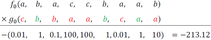
A similar decomposition is possible for the L⁰ norm (also called Hamming distance), which is commonly used for the simulation of categorical variables. The Hamming distance measures the dissimilarity between two lists by counting the number of elements that have different categories (Hamming, 1950). Example the dissimilarity between $a,b,b,c,b,a$ and $a,c,b,a,c,a$ is $\mathrm{0},\mathrm{1},\mathrm{0},\mathrm{1},\mathrm{1},\mathrm{0}$ and the associated Hamming distance is 3.

$$\begin{array}{}\text{(3)}& {\mathit{\epsilon }}_{L^{\mathrm{0}}}\left(a,b\right)={\left(a-b\right)}^{\mathrm{0}}=\mathrm{1}-\sum _{j\in C}\left({\mathit{\delta }}_{a,j}.{\mathit{\delta }}_{b,j}\right)\propto \sum _{j\in C}{\mathit{\delta }}_{a,j}\cdot {\mathit{\delta }}_{b,j},\end{array}$$

where δ_x,y is the Kronecker delta between x and y, which is 1 if x equals y and 0 otherwise, and C is the set of all possible categories of a specified variable. Here J=C.

Using Eq. (1), this L⁰ distance can be decomposed (Arpat and Caers, 2007) into the following series of functions f_j and g_j:

$$\begin{array}{l}{f}_j:x\to -{\mathit{\delta }}_{xj}\\ g_j:x\to {\mathit{\delta }}_{xj}\end{array}$$

with a new pair of f_j and g_j for each class j of C.

For multivariate pixels, such as a combination of categorical and continuous values, the mismatch ε can be expressed as a sum of univariate pixelwise mismatches.

$$\begin{array}{}\text{(4)}& \mathit{\epsilon }\left(\mathit{a},\mathit{b}\right)\propto \sum _{i\in I}\sum _{j\in J_i}{f}_j\left(a_i\right)\cdot g_j\left(b_i\right),\end{array}$$

where a and b are the compared vectors and a_i and b_i are the individual components of a and b. J_i represents the set related to the metric used for the ith variable, and I represents the set of variables.

2.3 Computation of a mismatch map for an entire pattern

The approach that is proposed in this work is based on computing a mismatch map in the training image (TI) for each simulated pixel. The mismatch map is a grid that represents the patternwise mismatch for each location of the training image and enables the fast identification of a good candidate, as shown by the red circle in Fig. 1.

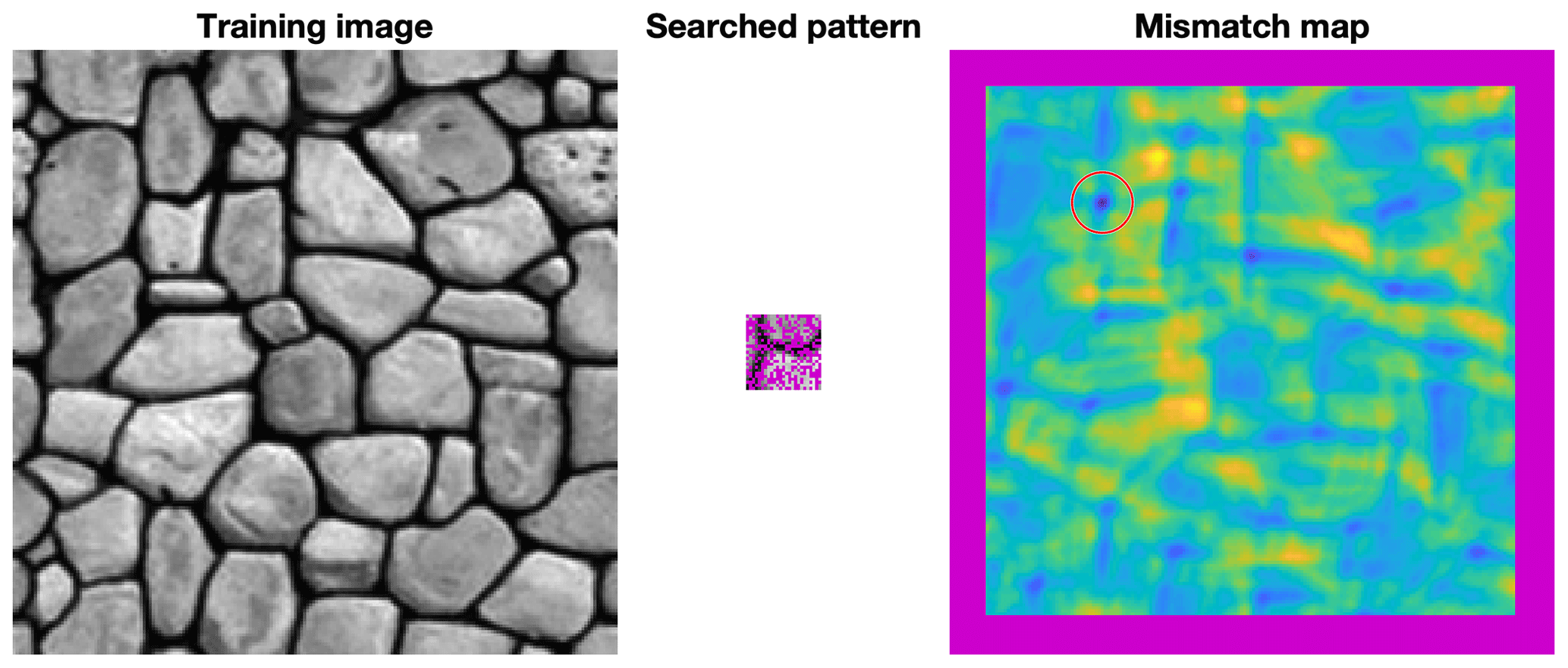
Figure 1 Example of a mismatch map for an incomplete pattern. Blue represents good matches, yellow bad matches, and purple missing and unusable (border effect) data. The red circle highlights the minimum of the mismatch map, which corresponds to the location of the best candidate.

If we consider the neighborhood N(s) around the simulated position s, then we can express a weighted dissimilarity between N(s) and a location in the training image N(t):

$$\begin{array}{}\text{(5)}& \mathrm{E}\left(N\left(t\right),N\left(s\right)\right)=\sum _{\mathit{l}\in N(t,s)}{\mathit{\omega }}_{\mathit{l}}\mathit{\epsilon }\left(N_{\mathit{l}}\left(t\right),N_{\mathit{l}}\left(s\right)\right),\end{array}$$

where $N\left(t,s\right)=\mathit{\{}l\mathrm{|}{N}_{\mathit{l}}\left(t\right)$, N_l(s) exists}, and N_l(p) represents the neighbors of p (p can represent either s or t) with a relative displacement l from p; therefore, N(p)={l | N_l(p)}, l is the lag vector that defines the relative position of each value within N, and ω_l is a weight for each pixelwise error according to the lag vector l. By extension, ω is the matrix of all weights, which we call the weighting kernel or, simply, the kernel. E represents the mismatch between patterns that are centered on s and t∈T, where T is the training image.

Some lags may not correspond to a value, for example, due to edge effects in the considered images or because the patterns are incomplete. Missing patterns are inevitable during the course of a simulation using a sequential path. Furthermore, in many instances, there can be missing areas in the training image. This is addressed by creating an indicator variable to be used as a mask, which equals 1 at informed pixels and 0 everywhere else:

$$\begin{array}{}\text{(6)}& {\text{𝟙}}_{\mathit{l}}\left(p\right)=\left\{\begin{array}{l}\mathrm{1}\text{if}{N}_{\mathit{l}}\left(p\right)\text{is}\text{informed}\\ \mathrm{0}\text{otherwise.}\end{array}\right.\end{array}$$

Let us first consider the case in which, for a specified position, either all or no variables are informed. Expressing the presence of data as a mask enables the gaps to be ignored, because the corresponding errors are multiplied by zero.

Then, Eq. (5) can be expressed as follows:

$$\begin{array}{}\text{(7)}& \begin{array}{rl}\mathrm{E}\left(N\left(t\right),N\left(s\right)\right)& =\sum _{\mathit{l}}{\mathit{\omega }}_{\mathit{l}}\cdot {\text{𝟙}}_{\mathit{l}}\left(t\right)\cdot {\text{𝟙}}_{\mathit{l}}\left(s\right)\\ & \cdot \mathit{\epsilon }\left(N_{\mathit{l}}\left(t\right),N_{\mathit{l}}\left(s\right)\right).\end{array}\end{array}$$

Combining Eqs. (4) and (7), we get

$$\begin{array}{}\text{(8)}& \begin{array}{rl}\mathrm{E}& \left(N\left(t\right),N\left(s\right)\right)\\ & \propto \sum _{\mathit{l}}{\mathit{\omega }}_{\mathit{l}}{\text{𝟙}}_{\mathit{l}}\left(t\right){\text{𝟙}}_{\mathit{l}}\left(s\right)\sum _{i\in I}\sum _{j\in J_i}{f}_j\left(N_{\mathit{l}}{\left(t\right)}_i\right)g_j\left(N_{\mathit{l}}{\left(s\right)}_i\right)\\ & =\sum _{\mathit{l}}\sum _{i\in I}\sum _{j\in J_i}{\mathit{\omega }}_{\mathit{l}}{\text{𝟙}}_{\mathit{l}}\left(t\right){\text{𝟙}}_{\mathit{l}}\left(s\right)f_j\left(N_{\mathit{l}}{\left(t\right)}_i\right)g_j\left(N_{\mathit{l}}{\left(s\right)}_i\right)\\ & =\sum _{i\in I}\sum _{j\in J_i}\sum _{\mathit{l}}{\mathit{\omega }}_{\mathit{l}}\left({\text{𝟙}}_{\mathit{l}}\left(t\right)f_j\left(N_{\mathit{l}}{\left(t\right)}_i\right)\right)\left({\text{𝟙}}_{\mathit{l}}\left(s\right)\right)\left(g_j\left(N_{\mathit{l}}{\left(s\right)}_i\right)\right)\\ & =\sum _{i\in I}\sum _{j\in J_i}\sum _{\mathit{l}}\left({\mathrm{1}}_{\mathit{l}}\left(t\right)f_j\left(N_{\mathit{l}}{\left(t\right)}_i\right)\right)\left({\mathit{\omega }}_{\mathit{l}}{\text{𝟙}}_{\mathit{l}}\left(s\right)\right.\left.g_j\left(N_{\mathit{l}}{\left(s\right)}_i\right)\right).\end{array}\end{array}$$

After rewriting, Eq. (8) can be expressed as a sum of cross-correlations that encapsulate spatial dependencies, using the cross-correlation definition, $f\star g=\sum _l{f}_l\cdot g_l$, as follows:

$$\begin{array}{}\text{(9)}& \begin{array}{rl}\mathrm{E}& \left(N\left(t\right),N\left(s\right)\right)\\ & \propto \sum _{i\in I}\sum _{j\in J_i}\left(\text{𝟙}\left(t\right)\circ f_j\left(N{\left(t\right)}_i\right)\right)\star \left(\mathit{\omega }\circ \text{𝟙}\left(s\right)\circ g_j\left(N{\left(s\right)}_i\right)\right),\end{array}\end{array}$$

where ω and 𝟙(.)  represent the matrices that are formed by ω_l and 𝟙_l(.) for all possible vectors l, ⋆ denotes the cross-correlation operator, and ^∘ is the element-wise product (or Hadamard product).

Finally, with $T=\left\{T_i,i\in I\right\}$, T_i represents the training image for the ith variable, and, by applying cross-correlations for all positions t∈T, we obtain a mismatch map, which is expressed as

$$\begin{array}{}\text{(10)}& \begin{array}{rl}\mathrm{E}& \left(T,N\left(s\right)\right)\\ & \propto \sum _{i\in I}\sum _{j\in J_i}\left(\mathrm{1}\left(T\right)\circ f_j\left(T_i\right)\right)\cdot \left(\mathit{\omega }\circ \mathrm{1}\left(s\right)\circ g_j\left(N{\left(s\right)}_i\right)\right).\end{array}\end{array}$$

The term 1(T) allows for the consideration of the possibility of missing data in the training image T.

Let us consider the general case in which only some variables are informed and the weighting can vary for each variable. Equation (10) can be extended for this case by defining separate masks and weights ω_i for each variable:

$$\begin{array}{}\text{(11)}& \begin{array}{rl}\mathrm{E}& \left(T,N\left(s\right)\right)\\ & \propto \sum _{i\in I}\sum _{j\in J_i}\left(\text{𝟙}\left(T_i\right)\circ f_j\left(T_i\right)\right)\star \left({\mathit{\omega }}_i\circ \text{𝟙}\left(s_i\right)\circ g_j\left(N{\left(s\right)}_i\right)\right).\end{array}\end{array}$$

Equation (11) can be expressed using the convolution theorem applied to cross-correlation:

$$\begin{array}{}\text{(12)}& \begin{array}{rl}\mathrm{E}& \left(T,N\left(s\right)\right)\\ & \propto \sum _{i\in I}\sum _{j\in J_i}{\mathcal{F}}^{-\mathrm{1}}\mathit{\{}\stackrel{\mathrm{‾}}{\mathcal{F}\left\{\mathrm{1}\left(T_i\right)\circ f_j\left(T_i\right)\right\}}\\ & \circ \mathcal{F}\left\{{\mathit{\omega }}_i\circ \mathrm{1}\left(s_i\right)\circ g_j\left(N{\left(s\right)}_i\right)\right\}\mathit{\}},\end{array}\end{array}$$

where ℱ represents the Fourier transform, ℱ⁻¹ the inverse transform, and $\stackrel{\mathrm{‾}}{x}$ the conjugate of x.

By linearity of the Fourier transform, the summation can be performed in Fourier space, thereby reducing the number of transformations:

$$\begin{array}{}\text{(13)}& \begin{array}{rl}\mathrm{E}& \left(T,N\left(s\right)\right)\\ & \propto {\mathcal{F}}^{-\mathrm{1}}\mathit{\{}\sum _{i\in I}\sum _{j\in J_i}\stackrel{\mathrm{‾}}{\mathcal{F}\left\{\mathit{\text{𝟙}}\left(T_i\right)\circ f_j\left(T_i\right)\right\}}\\ & \circ \mathcal{F}\left\{{\mathit{\omega }}_i\circ \text{𝟙}\left(s_i\right)\circ g_j\left(N{\left(s\right)}_i\right)\right\}\mathit{\}}.\end{array}\end{array}$$

Equation (13) is appropriate for modern computers, which are well suited for computing FFTs (Cooley et al., 1965; Gauss, 1799). Currently, FFTs are well implemented in highly optimized libraries (Rodríguez, 2002). Equation (13) is the expression that is used in our QS implementation, because it reduces the number of Fourier transforms, which are the most computationally expensive operations of the algorithm. One issue with the use of FFTs is that the image T is typically assumed to be periodic. However, in most practical applications, it is not periodic. This can be simply addressed by cropping the edges of E(T,N(s)) or by adding a padding around T.

The computation of the mismatch map (Eq. 13) is deterministic; as a result, it incurs a constant computational cost that is independent of the pixel values. Additionally, Eq. (13) is expressed without any constraints on the dimensionality. Therefore, it is possible to use the n-dimensional FFTs that are provided in the above libraries to perform n-dimensional simulations without changing the implementation.

2.4 Selection of candidates based on a quantile

The second contribution of this work is the k-sampling strategy for selecting a simulated value among candidates. The main idea is to use the previously calculated mismatch map to select a set of potential candidates that are defined by the k smallest (i.e., a quantile) values of E. Once this set has been selected, we randomly draw a sample from this pool of candidates. This differs from strategies that rely on a fixed threshold, which can be cumbersome to determine. This strategy is highly similar to the ε-replicate strategy that is used in image quilting (Mahmud et al., 2014) in that we reuse and extend to satisfy the specific requirements of QS. It has the main advantage of rescaling the acceptance criterion according to the difficulty; i.e. the algorithm is more tolerant of rare patterns while requiring very close matches for common patterns.

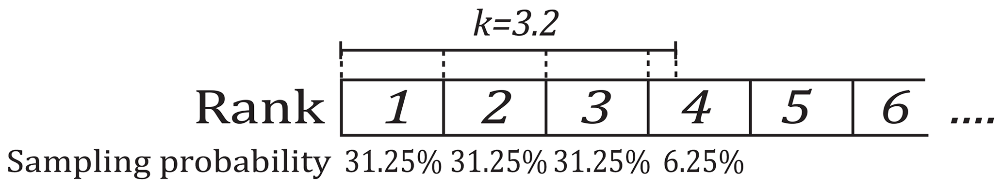
In detail, the candidate selection procedure is as follows: All possible candidates are ranked according to their mismatch, and one candidate is randomly sampled among the k best. This number, k, can be seen as a quantile over the training dataset. However, parameter k has the advantage of being an easy representation for users, who can associate k=1 with the best candidate, k=2 with the two best candidates, etc. For fine-tuning parameter k, the sampling strategy can be extended to non-integer values of k by sampling the candidates with probabilities that are not uniform. For example, if the user sets k=1.5, the best candidate has a probability of two-thirds of being sampled and the second best a probability of one-third. For k=3.2 (Fig. 2), each of the three best candidates are sampled with an equal probability of 0.3125 and the fourth best with a probability of 0.0625. This feature is especially useful for tuning k between 1 and 2 and for avoiding a value of k=1, which can result in the phenomenon of verbatim copy.

Figure 2 Illustration of the k-sampling strategy.

An alternative sampling strategy for reducing the simulation time is presented in Appendix A3. However, this strategy can result in a reduction in the simulation quality.

The value of non-integer k values is not only in the fine tuning of parameters. It also allows for direct comparisons between QS and DS. Indeed, under the hypothesis of a stationary training image, using DS with a given max fraction of scanned training image (f) and a threshold (t) of 0 is statistically similar to using QS with $k=\mathrm{1}/f$. In both situations, the best candidate is sampled in a fraction f of the training image.

2.5 Simplifications in the case of a fully informed training image

In many applications, spatially exhaustive TIs are available. In such cases, the equations above can be simplified by dropping constant terms from Eq. (1), thereby resulting in a simplified form for Eq. (13). Here, we take advantage of the ranking to know that a constant term will not affect the result.

As in Tahmasebi et al. (2012), in the L² norm, we drop the squared value of the searched pattern, namely b², from Eq. (2). Hence, we can express Eq. (4) as follows:

$$\begin{array}{}\text{(14)}& \mathit{\epsilon }\left(\mathit{a},\mathit{b}\right)=\sum _{i\in I}{a}_i^{\mathrm{2}}-\mathrm{2}\sum _{i\in I}{a}_i\cdot b_i.\end{array}$$

The term a², which represents the squared value of the candidate pattern in the TI, differs among training image locations and therefore cannot be removed. Indeed, the assumption that ∑a² is constant is only valid under a strict stationarity hypothesis on the scale of the search pattern. While this hypothesis might be satisfied in some cases (as in Tahmasebi et al., 2012), we do not believe it is generally valid. Via the same approach, Eq. (3) can be simplified by removing the constant terms; then, we obtain the following for the L⁰ norm:

$$\begin{array}{}\text{(15)}& \mathit{\epsilon }\left(\mathit{a},\mathit{b}\right)=-\sum _{i\in I}\sum _{j\in C}{\mathit{\delta }}_{a_i,j}\cdot {\mathit{\delta }}_{b_i,j}.\end{array}$$

2.6 Efficient implementation

An efficient implementation of QS was achieved by (1) performing precomputations, (2) implementing an optimal partial sorting algorithm for selecting candidates, and (3) optimal coding and compilation. These are described below.

According to Eq. (13), $\stackrel{\mathrm{‾}}{\mathcal{F}\left\{\mathrm{1}\left(T_i\right)\circ f_j\left(T_i\right)\right\}}$ is independent of the searched pattern N(s). Therefore, it is possible to precompute it at the initialization stage for all i and j. This improvement typically reduces the computation time for an MPS simulation by a factor of at least 2.

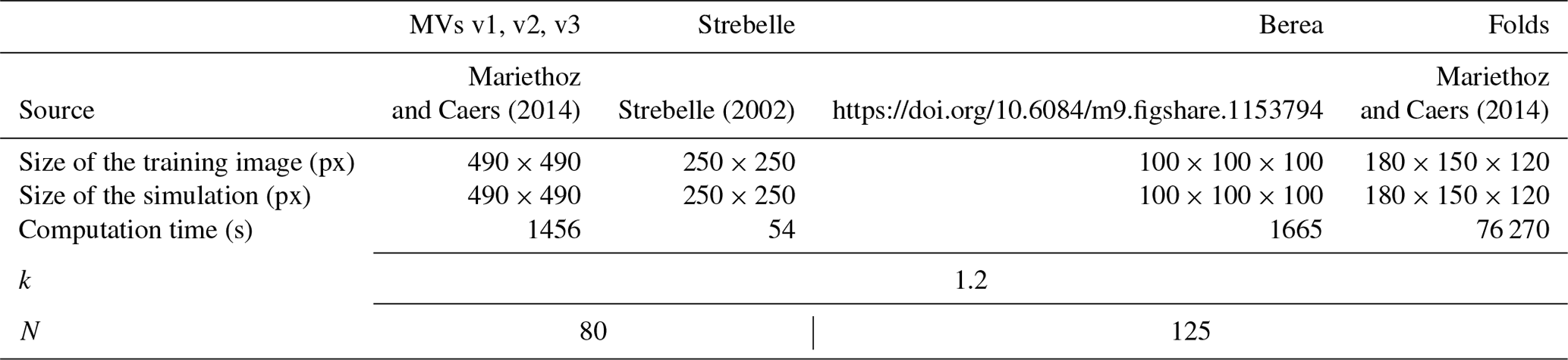
Table 1 Parameters that were used for the simulations in Fig. 3. Times are specified for simulations without parallelization. MVs represents multivariates.

Table 2 Hardware that was used in the experiments.

In the QS algorithm, a substantial part of the computation cost is incurred in identifying the k best candidates in the mismatch map. In the case of non-integer k, the upper limit ⌈k⌉ is used. Identifying the best candidates requires sorting the values of the mismatch map and retaining the candidates in the top k ranks. For this, an efficient sorting algorithm is needed. The operation of finding the k best candidates can be implemented with a partial sort, in which only the elements of interest are sorted while the other elements remain unordered. This results in two sets: S_s with the k smallest elements and S_l with the largest elements. The partial sort guarantees that $x\le y\mathrm{|}\left(x,y\right)\in S_{\mathrm{s}}\times S_{\mathrm{l}}$. More information about our implementation of this algorithm is available in Appendix A1. Here, we use a modified vectorized online heap-based partial sort (Appendix A1). With a complexity of O(nln (k)), it is especially suitable for small values of k. Using the cache effect, the current implementation yields results that are close to the search of the best value (the smallest value of the array). The main limitation of standard partial sort implementations is that in the case of equal values, either the first or the last element is sampled. Here, we develop an implementation that can uniformly sample a position among similar values with a single scan of the array. This is important because systematically selecting the same position for the same pattern will reduce the conditional probability density function to a unique sample, thereby biasing the simulation.

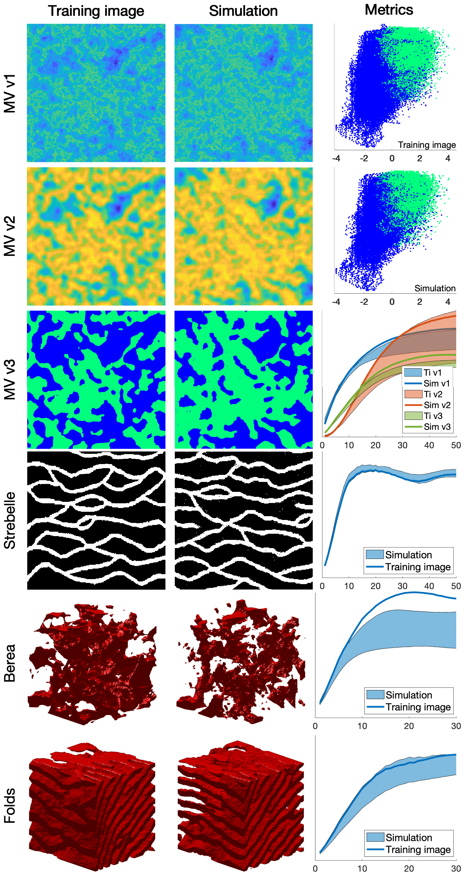
Figure 3 Examples of unconditional continuous and categorical simulations in 2D and 3D and their variograms. The first column shows the training images that were used, the second column one realization, and the third column quantitative quality metrics. MV v1, MV v2, and MV v3 represent a multivariate training image (and the corresponding simulation) using three variables. The first two metrics are scatter plots of MV v1 vs. MV v2 of the training image and the simulation, respectively. The third metric represents the reproduction of the variogram for each of MV v1, MV v2, and MV v3.

Due to the intensive memory access by repeatedly scanning large training images, interpreted programming languages, such as MATLAB and Python, are inefficient for a QS implementation and, in particular, for a parallelized implementation. We provide a NUMA-aware (Blagodurov et al., 2010) and flexible C/C$++$/OpenMP implementation of QS that is highly optimized. Following the denomination of Mariethoz (2010), we use a path-level parallelization with a waiting strategy, which offers a good trade-off between performance and memory requirements. In addition, two node-level parallelization strategies are available: if many training images are used, a first parallelization is performed over the exploration of the training images; then, each FFT of the algorithm is parallelized using natively parallel FFT libraries.

The FFTw library (Frigo and Johnson, 2018) provides a flexible and performant architecture-independent framework for computing n-dimensional Fourier transformations. However, an additional speed gain of approximately 20 % was measured by using the Intel MKL library (Intel Corporation, 2019) on compatible architectures. We also have a GPU implementation that uses clFFT for compatibility. Many Fourier transforms are sparse and, therefore, can easily be accelerated in n-dimensional cases with “partial FFT” since Fourier transforms of only zeros result in zeros.

3 Results

3.1 Simulation examples

This section presents illustrative examples for continuous and categorical case studies in 2D and in 3D. Additional tests are reported in Appendix A4. The parameters that are used for the simulations of Fig. 3 are reported in Table 1.

The results show that simulation results are consistent with what is typically observed with state-of-the-art MPS algorithms. While simulations can accurately reproduce TI properties for relatively standard examples with repetitive structures (e.g., MV, Strebelle, and Folds), training images with long-range features (typically larger than the size of the TI) are more difficult to reproduce, such as in the Berea example. For multivariate simulations, the reproduction of the joint distribution is satisfactory, as observed in the scatter plots (Fig. 3). More examples are available in Appendix A4, in particular Fig. A2 for 2D examples and Fig. A3 for 3D examples.

3.2 Comparison with direct sampling simulations

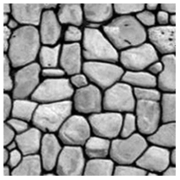
QS simulations are benchmarked against DS using the “Stone” training image (Fig. 4). The settings that are used for DS are based on optimal parameters that were obtained via the approach of Baninajar et al. (2019), which uses stochastic optimization to find optimal parameters. In DS, we use a fraction of scanned TI of f=1 to explore the entire training image via the same approach as in QS, and we use the L² norm as in QS. To avoid the occurrence of verbatim copy, we include 0.1 % conditioning data, which are randomly sampled from a rotated version of the training image. The number of neighbors N is set to 20 for both DS and QS and the acceptance threshold of DS is set to 0.001.

Figure 4 Training image that was used for benchmarking and sensitivity analysis.

The comparison is based on qualitative (Fig. 5) and quantitative (Fig. 6) metrics, which include directional and omnidirectional variograms, along with the connectivity function, the Euler characteristic (Renard and Allard, 2013), and cumulants (Dimitrakopoulos et al., 2010). The connectivity represents the probability for two random pixels to be in the same connected component. This metric is suited to detect broken structures. The Euler characteristic represents the number of objects subtracted by the number of holes of the objects, and is particularly adapted to detect noise in the simulations such as salt and pepper. Cumulants are high-order statistics and therefore allow for considering the relative positions between elements. The results demonstrate that the simulations are of a quality that is comparable to DS. With extreme settings (highest pattern reproduction regardless of the computation time), both algorithms perform similarly, which is reasonable since both are based on sequential simulation and both directly import data from the training image. The extra noise present in the simulation is shown in the Euler characteristic. Furthermore, it demonstrates that the use of a kernel can reduce this noise to get better simulations.

With QS, kernel weighting allows for fine tuning of the parametrization to improve the results, as shown in Fig. 8. In this paper, we use an exponential kernel:

$$\begin{array}{}\text{(16)}& {\mathit{\omega }}_{\mathit{l}}=e^{-\mathit{\alpha }{∥\mathit{l}∥}_{\mathrm{2}}},\end{array}$$

where α is a kernel parameter and ∥.∥₂ the Euclidean distance. The validation metrics of Fig 6 show that both QS and DS tend to slightly underestimate the variance and the connectivity. Figure 6 shows that an optimal kernel improves the results for all metrics, with all training image metrics in the 5 %–95 % realization interval, except for the Euler characteristic.

Figure 5 Examples of conditional simulations and their standard deviation over 100 realizations that are used in the benchmark between QS and DS.

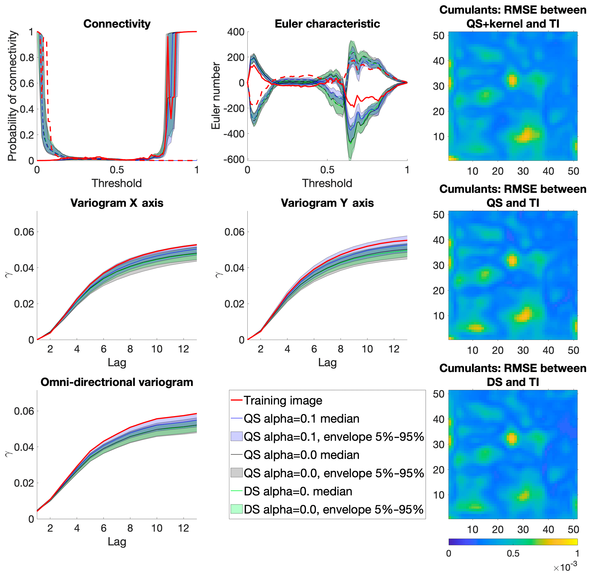
Figure 6 Benchmark between QS (with and without kernel) and DS over six metrics using each time 100 unconditional simulation.

3.3 Parameter sensitivity analysis

In this section, we perform a sensitivity analysis on the parameters of QS using the training image in Fig. 4. Only essential results are reported in this section (Figs. 7 and 8); more exhaustive test results are available in the appendix (Figs. A4 and A5). The two main parameters of QS are the number of neighbors N and the number of used candidates k.

Figure 7 (and Appendix Fig. A4) shows that large N values and small k values improve the simulation performance; however, they tend to induce verbatim copy in the simulation. Small values of N result in noise with good reproduction of the histogram.

ω can be a very powerful tool, typically using the assumption that the closest pixels are more informative than remote pixels. The sensitivity analysis of the kernel value α is explored in Figs. 8 and A5. They show that α provides a unique tool for improving the simulation quality. In particular, using a kernel can reduce the noise in simulations, which is clearly visible by comparing the Euler characteristic curves. However, reducing too much the importance of distant pixels results in ignoring them altogether and therefore damaging long-range structures.

3.4 Computational efficiency and scalability

In this section, we investigate the scalability of QS with respect to the size of the simulation grid, the size of the training image grid, the number of variables, incomplete training images, and hardware. According to the test results, the code will continue to scale with new-generation hardware.

As explained in Sect. 2.3 and 2.4, the amounts of time that are consumed by the two main operations of QS (finding candidates and sorting them) are independent of the pixel values. Therefore, the training image that is used is not relevant. (Here, we use simulations that were performed with the training image of Fig. 4 and its classified version for categorical cases.) Furthermore, the computation time is independent of the parametrization (k and N). However, the performance is affected by the type of mismatch function that is used; here, we consider both continuous (Eqs. 2 and 14) and categorical cases (Eqs. 3 and 15).

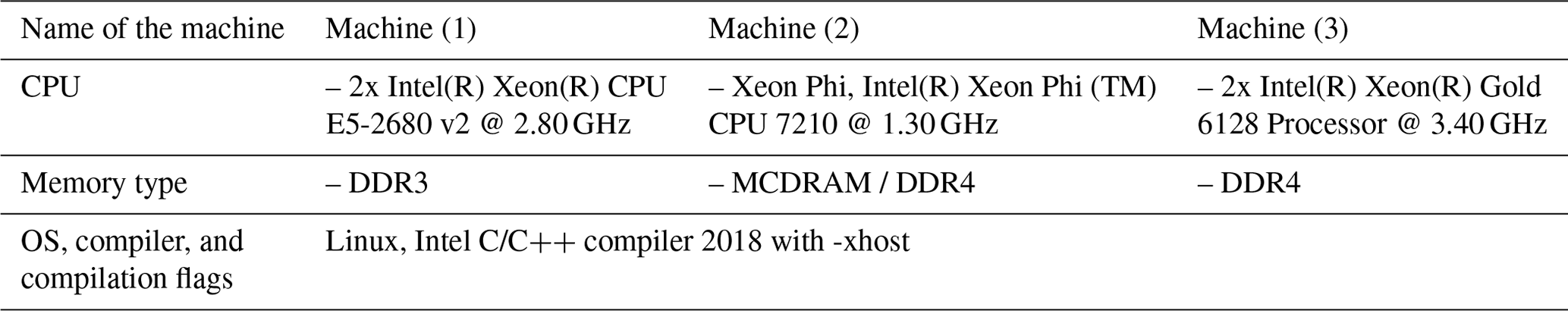
We also test our implementation on different types of hardware, as summarized in Table 2. We expect Machine (2) to be faster than Machine (1) for medium-sized problems due to the high-memory-bandwidth requirement of QS. Machine (3) should also be faster than Machine (1), because it takes advantage of a longer vector computation (512-bit vs. 256-bit instruction set).

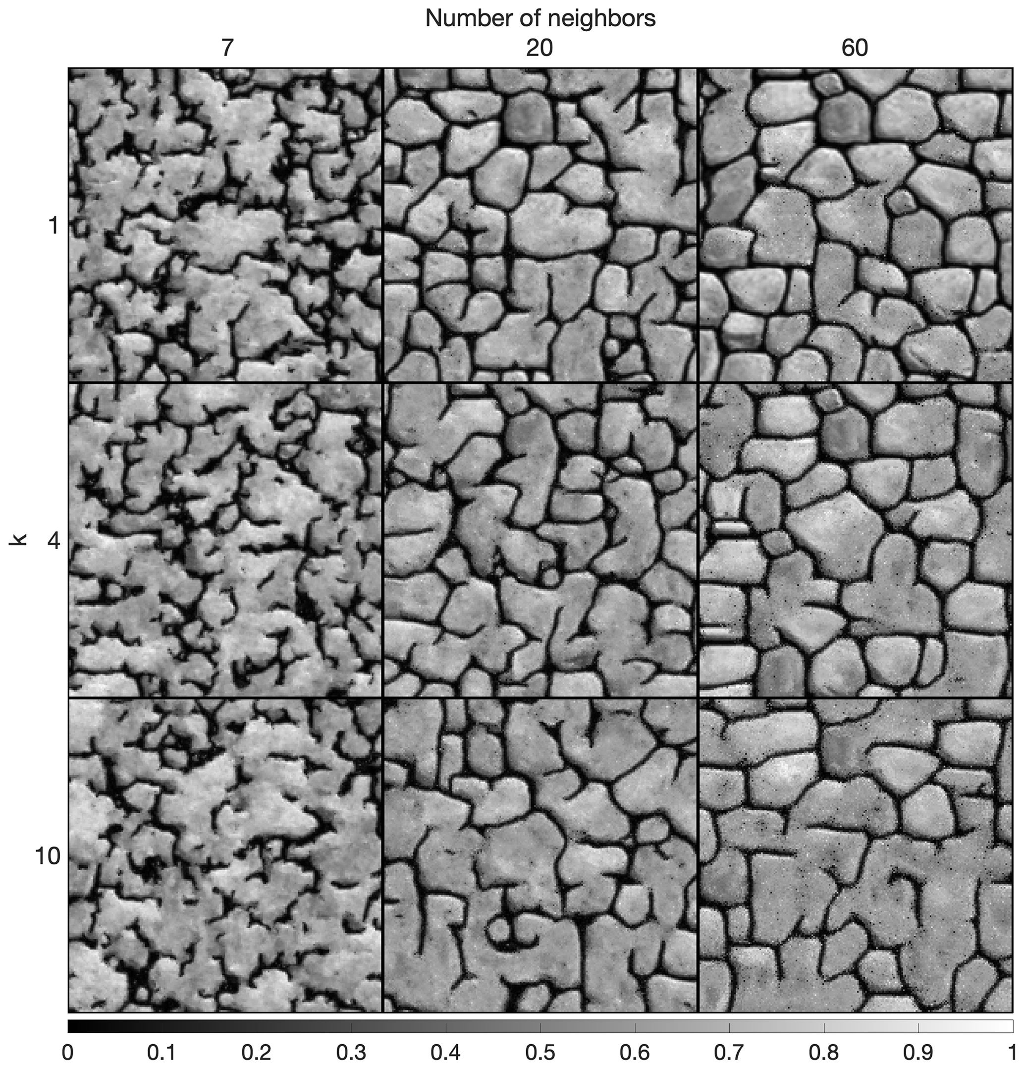
Figure 7 Sensitivity analysis on one simulation for the two main parameters of QS using a uniform kernel.

Figure 9 plots the execution times on the three tested machines for continuous and categorical cases and with training images of various sizes. Since QS has a predictable execution time, the influence of the parameters on the computation time is predictable: linear with respect to the number of variables (Fig. 9a, b), linear with respect to the size of the simulation grid, and following a power function of the size of the training image (Fig. 9c). Therefore, via a few tests on a set of simulations, one can predict the computation time for any other setting.

Figure 9d shows the scalability of the algorithm when using the path-level parallelization. The algorithm scales well until all physical cores are being used. Machine (3) has a different scaling factor (slope). This suboptimal scaling is attributed to the limited memory bandwidth. Our implementation of QS scales well with an increasing number of threads (Fig. 9d), with an efficiency above 80 % using all possible threads. The path-level parallelization strategy that was used involves a bottleneck for large numbers of threads due to the need to wait for neighborhood conflicts to be resolved (Mariethoz, 2010). This effect typically appears for large values of N or intense parallelization (>50 threads) on small grids. It is assumed that small grids do not require intense parallelization; hence, this problem is irrelevant in most applications.

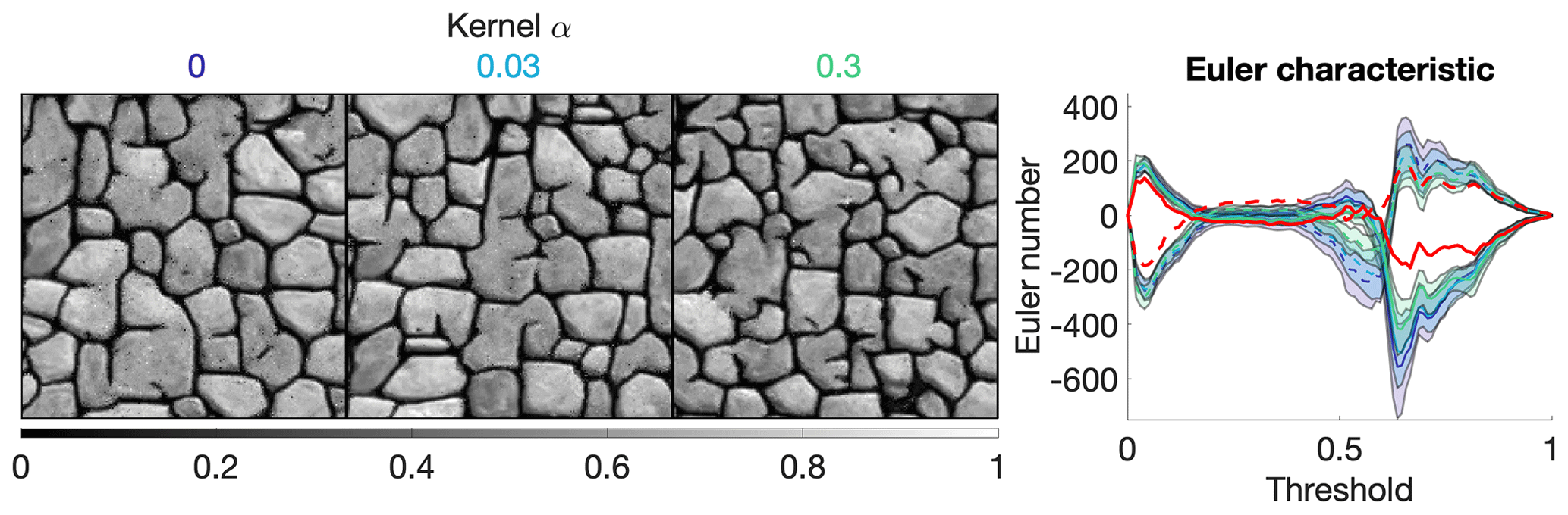
Figure 8 Sensitivity analysis on the kernel parameter α, with fixed parameters k=1.5 and N=40. The values of the kernels are shown in colors that correspond to the Euler characteristic lines (red is the training image).

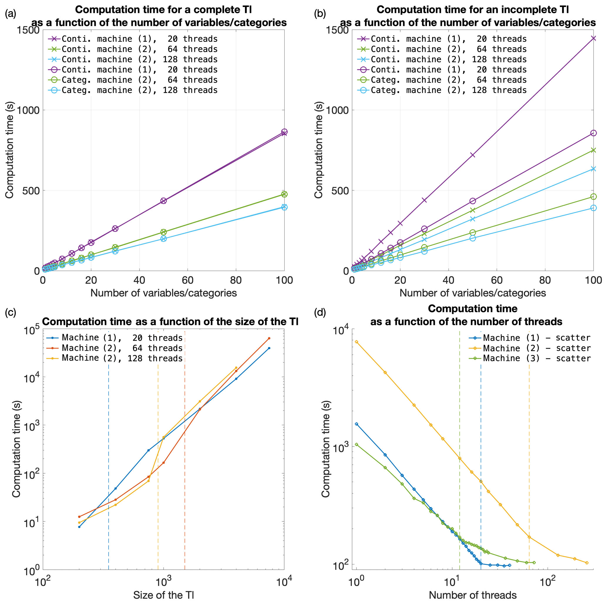
Figure 9 Efficiency of QS with respect to all key parameters. Panels (a) and (b) are the evolution of the computation time for complete and incomplete training images, respectively, with continuous and categorical variables. Panel (c) shows the evolution of the computation time as the size of the training image is varied; the dashed lines indicate that the training image no longer fits in the CPU cache. Panel (d) shows the evolution of the computation time as the number of threads is increased. The dashed lines indicate that all physical cores are used.

4 Discussion

The parametrization of the algorithm (and therefore simulation quality) has almost no impact on the computational cost, which is an advantage. Indeed, many MPS algorithms impose trade-offs between the computation time and the parameters that control the simulation quality, thereby imposing difficult choices for users. QS is comparatively simpler to set up in this regard. In practice, a satisfactory parametrization strategy is often to start with a small k value (say 1.2) and a large N value (>50) and then gradually change these values to increase the variability if necessary (Fig. 6 and A4).

QS is adapted for simulating continuous variables using the L² norm. However, a limitation is that the L¹ norm does not have a decomposition that satisfies Eq. (1), and therefore it cannot be used with QS. Another limitation is that for categorical variables, each class requires a separate FFT, which incurs an additional computational cost. This renders QS less computationally efficient for categorical variables (if there are more than two categories) than for continuous variables. For accelerated simulation of categorical variables, a possible alternative to reduce the number of required operations is presented in Appendix A2. The strategy is to use encoded variables, which are decoded in the mismatch map. While this alternative yields significant computational gains, it does not allow for the use of a kernel weighting and is prone to numerical precision issues.

Combining multiple continuous and categorical variables can be challenging for MPS approaches. Several strategies have been developed to overcome this limitation, using either a different distance threshold for each variable or a linear combination of the errors. Here we use the second approach, taking advantage of the linearity of the Fourier transform. The relative importance can be set in f_i and g_i functions in Eq. (1). However, it is computationally advantageous to use the kernel weights in order to have standard functions for each metric. Setting such variable-dependent parameters is complex. Therefore, in order to find optimal parameters, stochastic optimization approaches (such as Baninajar et al., 2019) are applied to QS. The computational efficiency of QS is generally advantageous compared to other pixel-based algorithms: for example, in our tests it performed faster than DS. QS requires more memory than DS, especially for applications with categorical variables with many classes and with a path-level parallelization. However, the memory requirement is much lower compared to MPS algorithms that are based on a pattern database, such as SNESIM.

There may be cases where QS is slower than DS, in particular when using a large training image that is highly repetitive. In such cases, using DS can be advantageous as it must scan only a very small part of the training image. For scenarios of this type, it is possible to adapt QS such that only a small subset of the training image is used; this approach is described in Appendix A3. In the cases of highly repetitive training images, this observation remains true also for SNESIM and IMPALA.

Furthermore, QS is designed to efficiently handle large and complex training images (up to 10 million pixels), with high variability of patterns and few repetitions. Larger training images may be computationally burdensome, which could be alleviated by using a GPU implementation thus allowing gains up to 2 orders of magnitude.

QS can be extended to handle the rotation and scaling of patterns by applying a constant rotation or affinity transformation to the searched patterns (Strebelle, 2002). However, the use rotation-invariant distances and affinity-invariant distances (as in Mariethoz and Kelly, 2011), while possible in theory, would substantially increase the computation time. Mean-invariant distances can be implemented by simply adapting the distance formulation in QS. All these advanced features are outside the scope of this paper.

5 Conclusions

QS is an alternative approach for performing n-dimensional pixel-based simulations, which uses an L² distance for continuous cases and an L⁰ distance for categorical data. The framework is highly flexible and allows other metrics to be used. The simple parametrization of QS renders it easy to use for nonexpert users. Compared to other pixel-based approaches, QS has the advantage of generating realizations in constant and predictable time for a specified training image size. Using the quantile as a quality criterion naturally reduces the small-scale noise compared to DS. In terms of parallelization, the QS code scales well and can adapt to new architectures due to the use of external highly optimized libraries.

The QS framework provides a complete and explicit mismatch map, which can be used to formulate problem-specific rules for sampling or even solutions that take the complete conditional probability density function into account, e.g., a narrowness criterion for the conditional probability density function of the simulated value (Gravey et al., 2019; Rasera et al., 2020), or to use the mismatch map to infer the optimal parameters of the algorithm.

Appendix A

A1 Partial sorting with random sampling

Standard partial sorting algorithms resolve tie ranks deterministically, which does not accord with the objective of stochastic simulation with QS, where variability is sought. Here, we propose an online heap-based partial sort. It is realized with a single scan of the array of data using a heap to store previously found values. This approach is especially suitable when we are interested in a small fraction of the entire array.

Random positions of the k best values are ensured by swapping similar values. If k=1, the saved value is switched with a smaller value each time it is encountered. If an equal value is scanned, a counter c is increased for this specific value and a probability of 1∕c of switching to the new position is applied. If k>1, the same strategy is extended by carrying over the counter c.

This partial sort outperforms random exploration of the mismatch map. However, it is difficult to implement efficiently on GPUs. A solution is still possible for shared-memory GPUs by performing the partial sort on the CPU. This is currently available in the proposed implementation.

• k: the number of value of interest

• D: the input data array

• S: the array with the k smallest value (sorted)

• Sp: the array with the positions that are associated with the values of S

1. for each value v of D

2. if v is smaller than the smallest value of S

3. search in S for the position p at which to insert v and insert it

4. if p=k // last position of the array

   • reinitialize the counter c to 0

   • insert v at the last position

   else

   • increment c by one

   • swap the last position with another of the same value

   • insert the value at the expected position p

   end

5. else if v is equal to the smallest value of S

   • increment c by one

   • change the position of v to one of the n positions of equal value with a probability of $n/(n+c)$

6. end

7. end

A2 Encoded categorical variables

To handle categorical variables, a standard approach is to consider each category as an independent variable. This requires as many FFTs as classes. This solution renders it expensive to use QS in cases with multiple categories.

An alternative approach is to encode the categories and to decode the mismatch from the cross-correlation. It has the advantage of only requiring only a single cross-correlation for each simulated pattern.

Here, we propose encoding the categories as powers of the number of neighbors, such that their product is equal to one if the class matches. In all other cases, the value is smaller than one or larger than the number of neighbors.

$$\begin{array}{}\text{(A1)}& {\mathit{\epsilon }}_{L^{\mathrm{0}}}\left(a,b\right)=\mathit{\psi }\left({\left(a-b\right)}^{\mathrm{0}}\propto -{\left(N+\mathrm{1}\right)}^{-p\left(a\right)}\cdot {\left(N+\mathrm{1}\right)}^{-p\left(b\right)}\right),\end{array}$$

where N is the largest number of neighbors that can be considered and p(c)  is an arbitrary function that maps index classes of C, c∈C.

In this scenario, in Eq. (1) this encoded distance $L_{\mathrm{e}}^{\mathrm{0}}$ can be decomposed into the following series of functions f_j and g_j:

$$\begin{array}{l}{f}_{\mathrm{0}}:x\to -{\left(N+\mathrm{1}\right)}^{p\left(x\right)}\\ g_{\mathrm{0}}:x\to {\left(N+\mathrm{1}\right)}^{-p\left(x\right)}\end{array}$$

and the decoding function is

$$\begin{array}{}\text{(A2)}& \mathit{\psi }\left(x\right)=⌊x⌋\mathrm{mod}N.\end{array}$$

Table A1 describes this process for three classes, namely a, b, and c, and a maximum of nine neighbors. Then, the error can be easily decoded by removing decimals and dozens.

Consider the following combination:

The decoding $⌊-\mathrm{213.12}⌋\mathrm{mod}\mathrm{10}=-\mathrm{213}\mathrm{mod}\mathrm{10}=-\mathrm{3}$ yields three matches (in green).

This encoding strategy provides the possibility of drastically reducing the number of FFT computations. However, the decoding phase is not always implementable if a nonuniform matrix ω is used. Finally, the test results show that the method suffers quickly from numerical precision issues, especially with many classes.

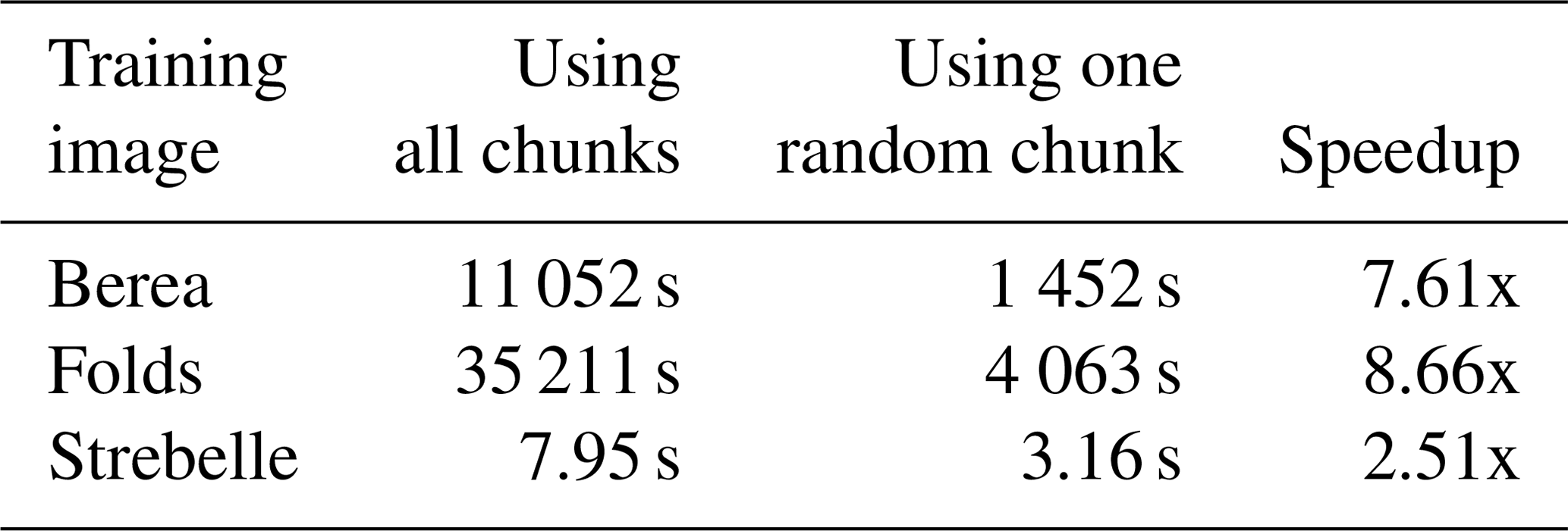
A3 Sampling strategy using training image splitting

The principle of considering a fixed number of candidates can be extended by, instead of taking the kth best candidate, sampling the best candidate in only a portion, $\frac{\mathrm{1}}{k}$, of the TI. For instance, as an alternative to considering k=4, this strategy searches for the best candidate in one-fourth of the image. This is more computationally efficient. However, if all the considered candidates are contiguous (by splitting the TI in k chunks), this approximation is only valid if the TI is completely stationary and all k equal subdivisions of the TI are statistically identical. In practice, real-world continuous variables are often nonstationary. However, in categorical cases, especially in binary ones, the number of pattern replicates is higher and this sampling strategy could be interesting.

The results of applying this strategy are presented in Table A2 and Fig. A1. The experimental results demonstrate that the partial exploration approach that is provided by splitting substantially accelerates the processing time. However, Fig. A1 shows that the approach has clear limitations when dealing with training images with complex and nonrepetitive patterns. The absence of local verbatim copy can explain the poor-quality simulation results.

Table A1 Example of encoding for three classes and nine neighbors and their associated products. The emboldened main diagonal shows the situations when the search classes match their corresponded values.

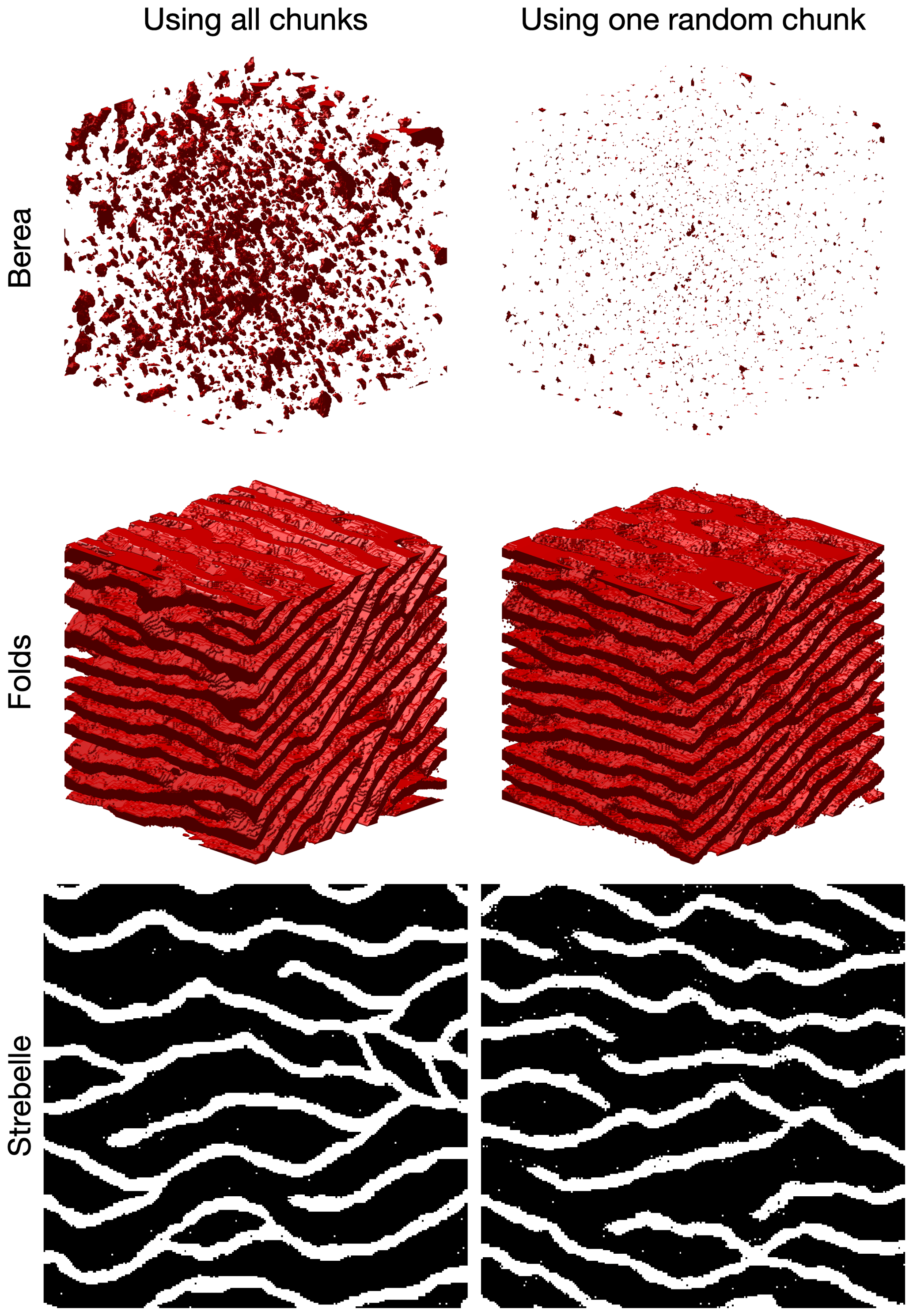
Figure A1 Comparison of QS using the entire training image and using training image splitting. In these examples, the training image is split into two images over each dimension. The original training images are presented in Fig. 2.

Table A2 Computation times and speedups for the full and partial exploration approaches. Times are specified for simulations with path-level parallelization.

A4 Additional results

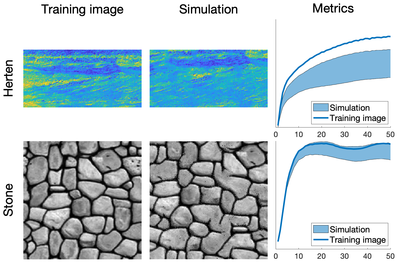
Figure A2 Examples of 2D simulations: the first three rows represent three variables of a single simulation. Parameters available in Table A3.

Figure A3 Examples of 3D simulation results. Parameters available in Table A4.

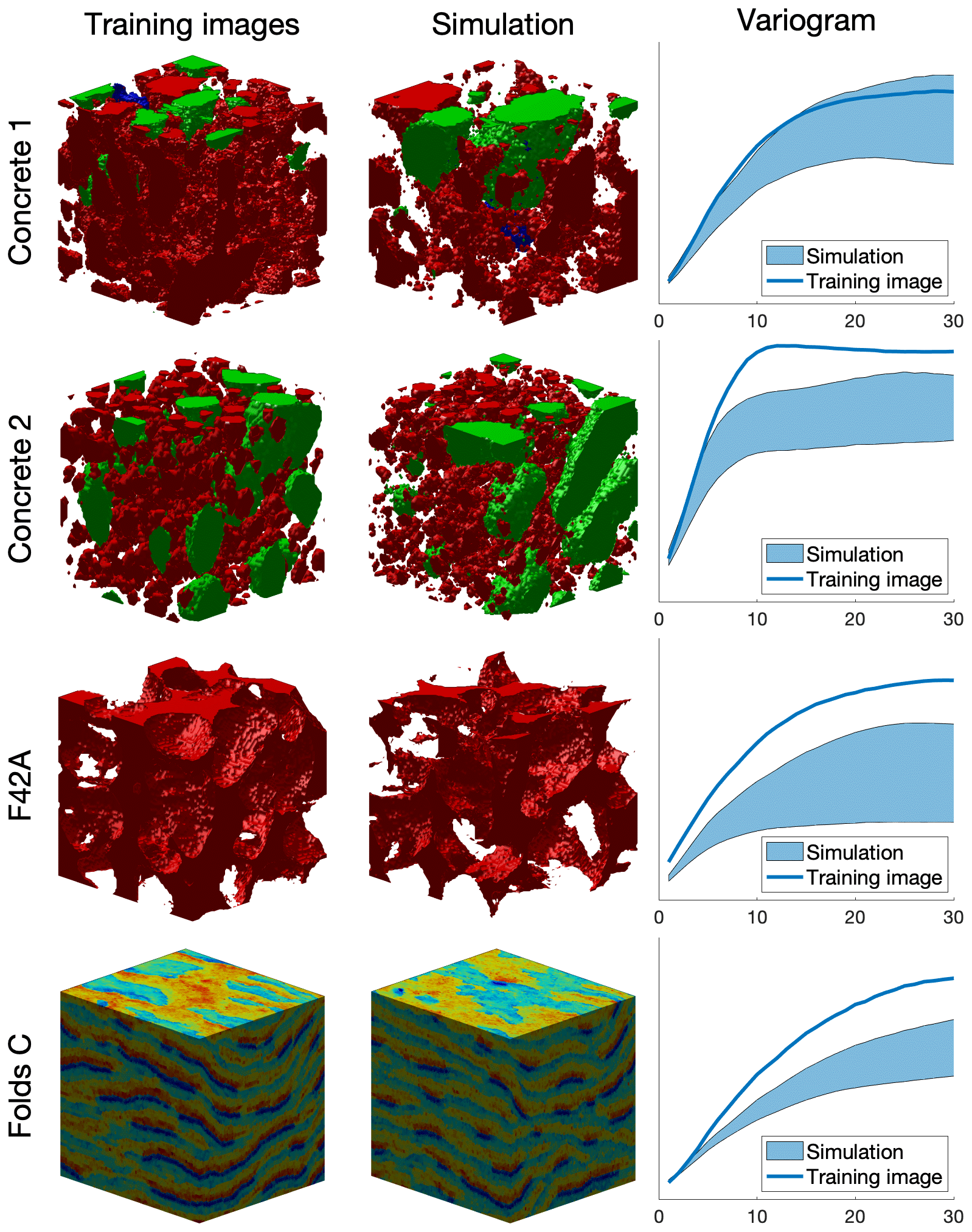
Table A3 Simulation parameters for Fig. A2. Times are specified for simulations without parallelization.

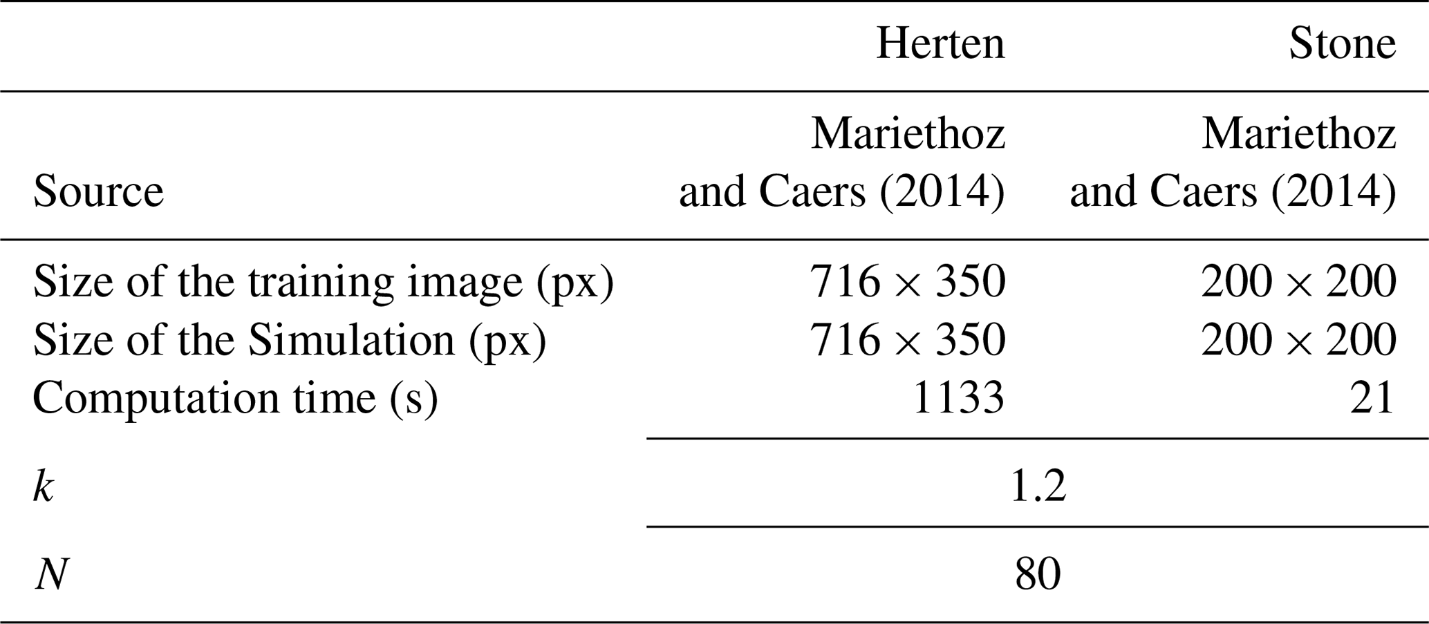
Table A4 Simulation parameters for Fig. A3. Times are specified for simulations without parallelization.

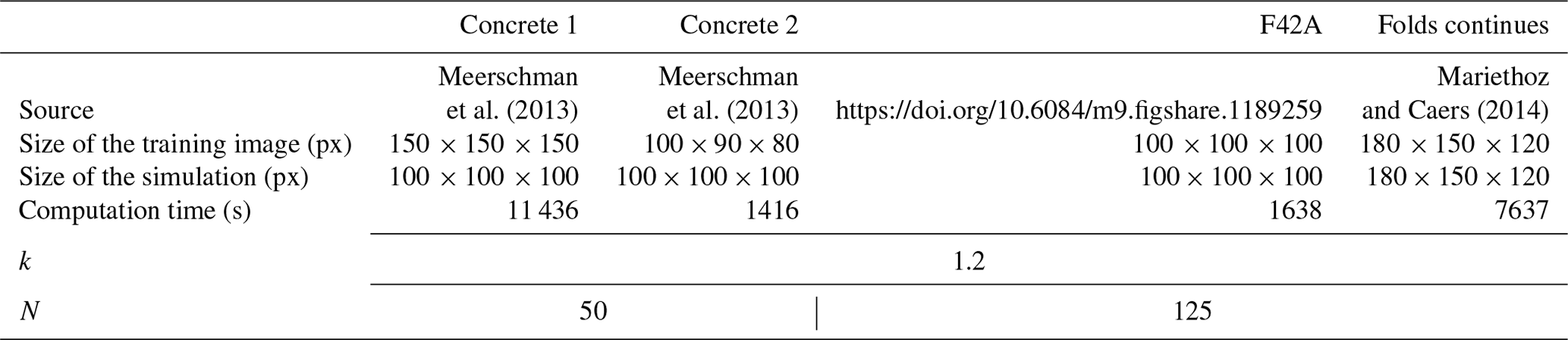
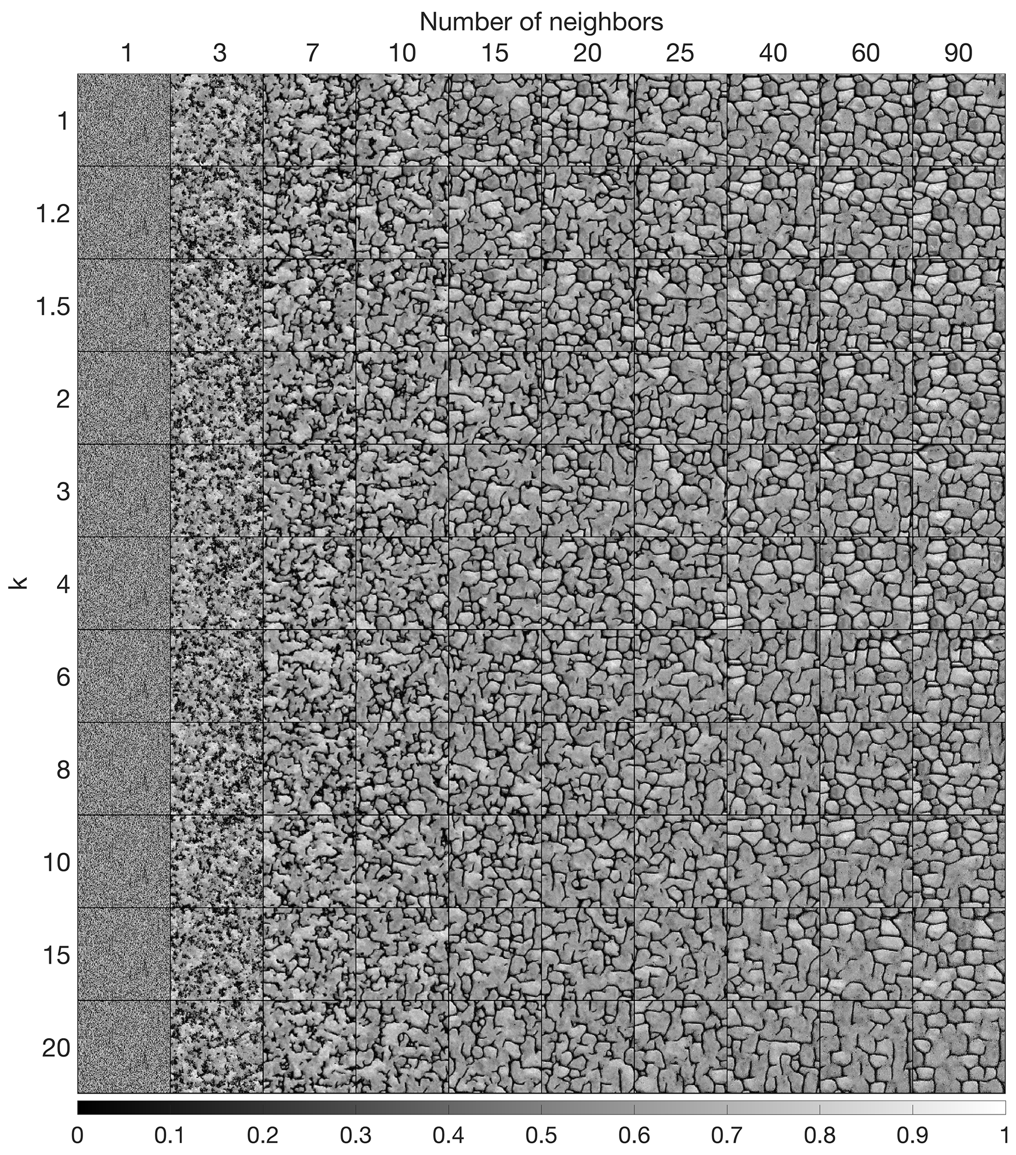
Figure A4 Complete sensitivity analysis, with one simulation for the two main parameters of QS.

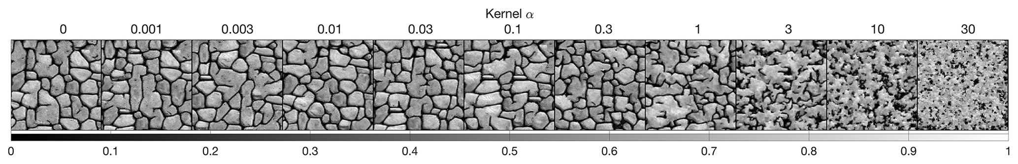
Figure A5 Complete sensitivity analysis, with one simulation for each kernel with k=1.5 and N=40.

A5 Mathematical derivation

The convolution theorem (Stockham, 1966; Krant, 1999; Li and Babu, 2019) can be easily extended to cross-correlation (Bracewell, 2000). The flowing derivation shows the validity of the theorem for any function f and g.

$$\begin{array}{}\text{(A3)}& \begin{array}{rl}F\left\{f\star g\right\}& =\int \left(f\star g\right)\left(t\right)e^{it\cdot \mathit{\xi }}\mathrm{d}t\\ & =\int \int \stackrel{\mathrm{‾}}{f\left(s\right)}g(s+t)\mathrm{d}s{e}^{it\cdot \mathit{\xi }}\mathrm{d}t\\ & =\int \int \stackrel{\mathrm{‾}}{f\left(s\right)}{e}^{i\left(-s\right)\cdot \mathit{\xi }}\mathrm{d}s\cdot g(s+t)\mathrm{d}s{e}^{i(t+s)\cdot \mathit{\xi }}\mathrm{d}t\\ & =\int \int \stackrel{\mathrm{‾}}{f\left(s\right)e^{i\left(s\right)\cdot \mathit{\xi }}}\mathrm{d}s\cdot g(s+t)\mathrm{d}s{e}^{i(t+s)\cdot \mathit{\xi }}\mathrm{d}t\\ & =\stackrel{\mathrm{‾}}{F\left\{f\right\}}\cdot F\left\{g\right\}\end{array}\end{array}$$

The discretization of this property can be obtained using two piecewise continuous functions associated with each discrete representation.