the Creative Commons Attribution 4.0 License.
the Creative Commons Attribution 4.0 License.
 | 29 Jan 2020
Turbulent kinetic energy over large offshore wind farms observed and simulated by the mesoscale model WRF (3.8.1)
Simon K. Siedersleben
Andreas Platis
Julie K. Lundquist
Bughsin Djath
Astrid Lampert
Konrad Bärfuss
Beatriz Cañadillas
Johannes Schulz-Stellenfleth
Jens Bange
Tom Neumann
Stefan Emeis
Wind farms affect local weather and microclimates; hence, parameterizations of their effects have been developed for numerical weather prediction models. While most wind farm parameterizations (WFPs) include drag effects of wind farms, models differ on whether or not an additional turbulent kinetic energy (TKE) source should be included in these parameterizations to simulate the impact of wind farms on the boundary layer. Therefore, we use aircraft measurements above large offshore wind farms in stable conditions to evaluate WFP choices. Of the three case studies we examine, we find the simulated ambient background flow to agree with observations of temperature stratification and winds. This agreement allows us to explore the sensitivity of simulated wind farm effects with respect to modeling choices such as whether or not to include a TKE source, horizontal resolution, vertical resolution and advection of TKE. For a stably stratified marine atmospheric boundary layer (MABL), a TKE source and a horizontal resolution on the order of 5 km or finer are necessary to represent the impact of offshore wind farms on the MABL. Additionally, TKE advection results in excessively reduced TKE over the wind farms, which in turn causes an underestimation of the wind speed deficit above the wind farm. Furthermore, using fine vertical resolution increases the agreement of the simulated wind speed with satellite observations of surface wind speed.
- Article
(7114 KB) - Full-text XML
- BibTeX
- EndNote


This work was authored in part by the National Renewable Energy Laboratory, operated by Alliance for Sustainable Energy, LLC, for the U.S. Department of Energy (DOE) under Contract No. DE-AC36-08GO28308. The U.S. Government retains and the publisher, by accepting the article for publication, acknowledges that the U.S. Government retains a nonexclusive, paid-up, irrevocable, worldwide license to publish or reproduce the published form of this work, or allow others to do so, for U.S. Government purposes.
Offshore wind energy in Europe has gained importance every year in the last decade. In 2017, the wind energy market experienced a new record in investments, with 3148 MW additional net installed offshore energy equal to 560 new offshore wind turbines at 17 wind farms. Two-thirds of these turbines were installed at the North Sea, equal to an increase of 2105 MW in net installed capacity (WindEurope, 2017).
Compared to onshore wind farms, offshore wind farms are larger in size; hence, the efficiency of large offshore wind farms is mainly driven by the turbulent vertical momentum flux (e.g., Emeis, 2010, 2018). Wind turbines extract kinetic energy from the mean flow and convert it partly into electrical energy. The resulting wind deficit downwind is balanced by the advection of momentum of the mean flow and the turbulent momentum fluxes. Within large wind farms, the kinetic energy deficit is mostly balanced by the vertical momentum flux as the inner turbines are surrounded by wind turbines extracting the kinetic energy from the mean horizontal flow. Given generally low mean vertical velocities on the mesoscale, the turbulent vertical momentum flux is crucial when determining the power density of large offshore wind farms.
Climate simulations and weather models investigating the impact of wind farms have a horizontal grid too coarse to resolve wind turbines explicitly. Therefore, these studies are all based on models using wind farm parameterizations (WFPs). In the past, areas of wind farms were represented as areas with increased surface roughness (Ivanova and Nadyozhina, 2000; Keith et al., 2004). Recently, wind turbines are parameterized as an elevated momentum sink at the levels intersecting with the rotor area (Fitch et al., 2012; Volker et al., 2015). Additionally, the WFP of Fitch et al. (2012) adds turbulent kinetic energy (TKE) at the rotor area, whereas the WFP of Volker et al. (2015) suggests that the TKE should be allowed to develop due to the resolved shear. However, both WFPs deliver similar results when calculating the power density (Volker et al., 2017).
Whether or not TKE enhancements should be included when using wind farm parameterizations to estimate impacts of wind farms is still a matter of debate. Several studies based on simulations (e.g., Eriksson et al., 2015; Vanderwende et al., 2016) suggest that the wind farm parameterization of Fitch et al. (2012) adds too much TKE into the model, causing exaggerated mixing, while Vanderwende et al. (2016) also point out that removing TKE completely results in poor agreement with large-eddy simulations of wind farms. However, an accurate representation of observed TKE and the associated change in the vertical fluxes over a wind farm is difficult to evaluate but necessary.
In this study, we present aircraft observations taken approximately 60 m above large offshore wind farms at the North Sea in the framework of the project Wind Park Far Field (WIPAFF) (Emeis et al., 2016), measuring the wind speed and the TKE above two different wind farms. We use these data to evaluate the wind farm parameterization of Fitch et al. (2012) for three real case studies. More specifically, we try to find answers to the following research questions:
-
Do wind farm parameterizations for mesoscale models need a TKE source to resolve the enhanced TKE above wind farms?
-
How sensitive is the impact of the wind farm parameterization on the TKE to the horizontal and vertical grid of the driving model?
-
How sensitive is the impact of the wind farm parameterization to the advection of TKE?
Section 2 gives an overview about the aircraft data, the configuration of the Weather Research and Forecasting model (WRF) and the synthetic aperture radar (SAR) satellite data for our case study of 14 October 2017. Additionally, we summarize the wind farm parameterization of Fitch et al. (2012). We present the synoptic and atmospheric conditions during the three case studies in Sect. 3. The measurements of the research aircraft are compared to the simulations in Sect. 4, followed by a sensitivity analysis with respect to the TKE source of the used WFP, horizontal and vertical grid resolution, and TKE advection in Sect. 5. Recommendations for mesoscale offshore wind farm simulations are finally discussed in Sect. 6.
Unique in situ aircraft measurements, described in Sect. 2.1, allow evaluation of the simulated marine atmospheric boundary layer (MABL) in the vicinity of the wind farms as well as TKE and wind speed over the wind farms. We have a SAR satellite image for one of the cases investigated in this study; a brief description of the SAR data is given in Sect. 2.2. In Sect. 2.3, the numerical model is presented, followed by a description of the wind farms (Sect. 2.4).
2.1 Aircraft measurements
In the framework of the WIPAFF project, the research aircraft Dornier 128-6 operated by TU Braunschweig was used for measuring the wakes of several large offshore wind farms within several campaigns. In these campaigns, the aircraft flew with a true air speed of 66 m s−1 on leveled and straight flight legs to measure wind speed, humidity, temperature and pressure at a sampling frequency of 100 Hz. Consequently, our measurements provide a data value every 0.66 m along the flight leg (Platis et al., 2018). Wind speed observations have a relative error of 1 % during the flights above the wind farms and 10 % during the climb flights resulting from different sample sizes, i.e., 3000 data points during the flights above offshore wind farms and 300 data points during the climb flights (Platis et al., 2018; Siedersleben et al., 2018b). The errors in the wind speed measurements cause an error of ±3∘ in the wind direction shown in the vertical profiles in Sect. 3 (Siedersleben et al., 2018b). Details about the measurement devices installed on the Dornier 128-6 can be found in Corsmeier et al. (2001).
Three sets of aircraft observations are discussed herein, labeled as cases I, II and III, summarized in Table 1. The aircraft observations were conducted on 9 August (case study I), 14 October (case study II) and 15 October 2017 (case study III) at two different wind farm clusters (Fig. 1 and Sect. 2.4). The observations above the wind farms on 9 August and 14 October 2017 started at ≈14:15 UTC and lasted 35 and 52 min. The measurements on 15 October 2017 took place from 08:28 to 09:21 and 09:52 to 10:17 UTC. The different observational periods are summarized in Table 1.
All aircraft measurements were conducted using the same pattern. Before we started the measurements over the wind farms, the aircraft profiled the MABL in the vicinity of the wind farms of interest, followed by several flights over the wind farms oriented perpendicular to the large-scale synoptic forcing. During all observations, the aircraft overflew the wind farm at least four times. Case study III included two additional measurements over the wind farms of interest conducted 40 min after the first four flight legs (Table 1).
The measurements were executed at two different wind farms (Figs. 1 and 2) with two different rotor types (more details in Sect. 2.4). Therefore, different flight heights were necessary – the aircraft flew at 200 m for case study I and 250 m for case studies II and III over the wind farms (Fig. 3) Meerwind Süd Ost (MSO) and OWP Nordsee Ost (ONO), and Godewind 1, 2 (GW), respectively.
Table 1Date, time, number of flight legs above the wind farms, location and flight height during the airborne observations.
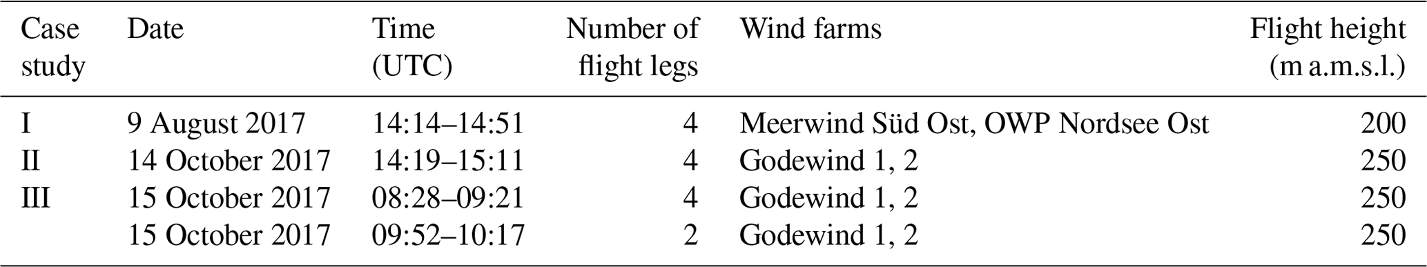
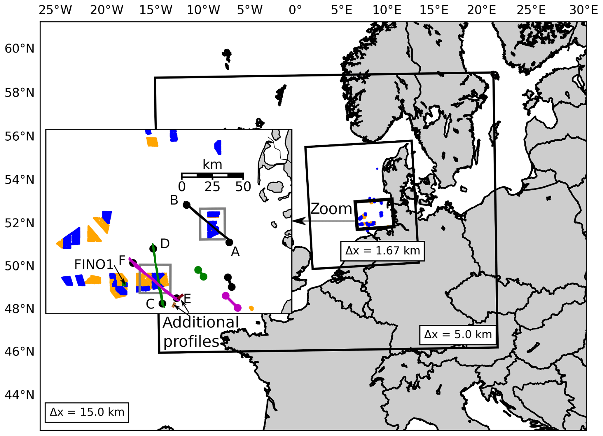
Figure 1Locations of WRF domains and wind farms at the North Sea. A close-up on the German Bight shows the wind farms of interest framed with gray rectangles and the flight tracks of the three measurements in black, green and magenta, corresponding to the measurements executed on 9 August, 14 and 15 October 2017, respectively. All measurements over the wind farms have a start and end point indicated with a capital letter for better orientation in Figs. 8, 10 and 11. Blue wind farms are operational; orange wind farms are approved or under construction during the time period investigated in this study. The thick lines indicate the locations of the climb flights, whereby the coloring corresponds to the coloring of the flight tracks over the wind farms, except the light red and red thick line showing the two additional profiles (see annotations) before and after the two additional flight legs. A detailed look (close-up on gray rectangles) at the wind turbine distribution of the wind farms of interest is provided in Fig. 2. The wind turbine location data were provided by the German Federal Maritime and Hydrographic Agency (BSH) and Bundesnetzagentur (2019).
2.2 SAR data
Active remote sensing sensors, such as satellite-borne SAR, have demonstrated the ability to provide 2-D mapping of spatial variation of offshore wind farm wakes (e.g., Christiansen and Hasager, 2005; Li et al., 2014; Hasager et al., 2005, 2015; Djath et al., 2018; Ahsbahs et al., 2018) due to the large coverage and spatial resolution of a few meters. Indeed, based on Bragg scattering principle, SAR captures the small-scale sea surface roughness, which is strongly related to wind conditions and returns the normalized radar cross section (NRCS). The combination of the C-band SAR satellite Sentinel-1A (launched in April 2014) and its twin Sentinel-1B (since April 2016) provides continuous measurements of the sea surface roughness of the German Bight with a repeat cycle of 6 d, but the same region can be sampled after 1 or 2 d with a different incidence angle. Due to its Sun-synchronous orbit, Sentinel-1 passes the German Bight at around 05:00 or 17:00 UTC. Figure 4a shows the 10 m wind speed derived from Sentinel-1A data acquired on 14 October 2017 at 17:17 UTC. The SAR scene is first calibrated to the NRCS using SNAP (Zuhlke et al., 2015) software supplied by European Space Agency. Then, the 10 m wind speed is derived using the geophysical model function CMOD5N (Hersbach et al., 2007; Verhoef et al., 2008) and hourly wind direction from German Weather Service (DWD) forecast model. The detailed methodology for the data processing and wind retrieval is described in Djath et al. (2018).
2.3 Numerical setup
All simulations were performed with the Weather Research and Forecasting Model WRF (version 3.8.1) (Skamarock et al., 2008). We used three domains, with 15 km in the outermost domain, followed by two domains with 5 and 1.67 km, respectively (Fig. 1). The boundary and initial conditions were provided by ERA5 data (Copernicus Climate Change Service, C3S, 2018), with a horizontal resolution of 0.25∘ and 138 vertical levels.
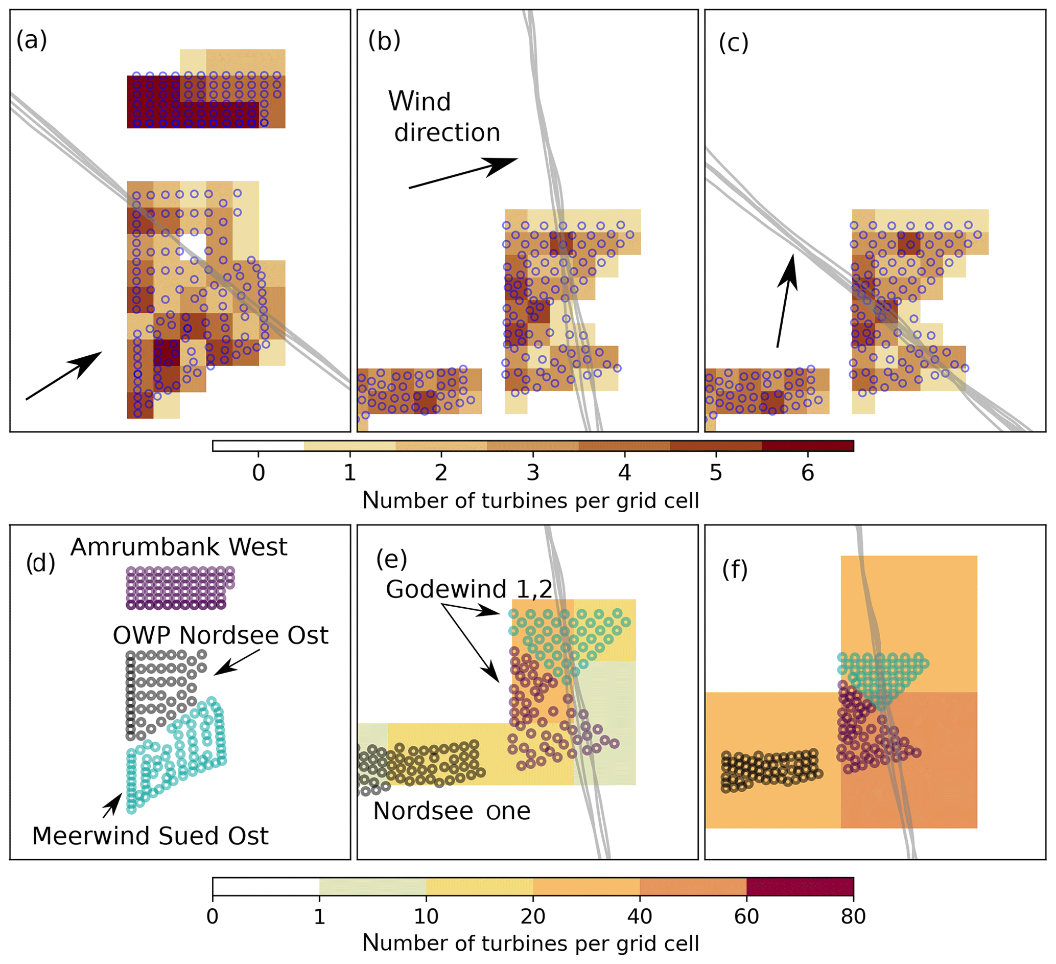
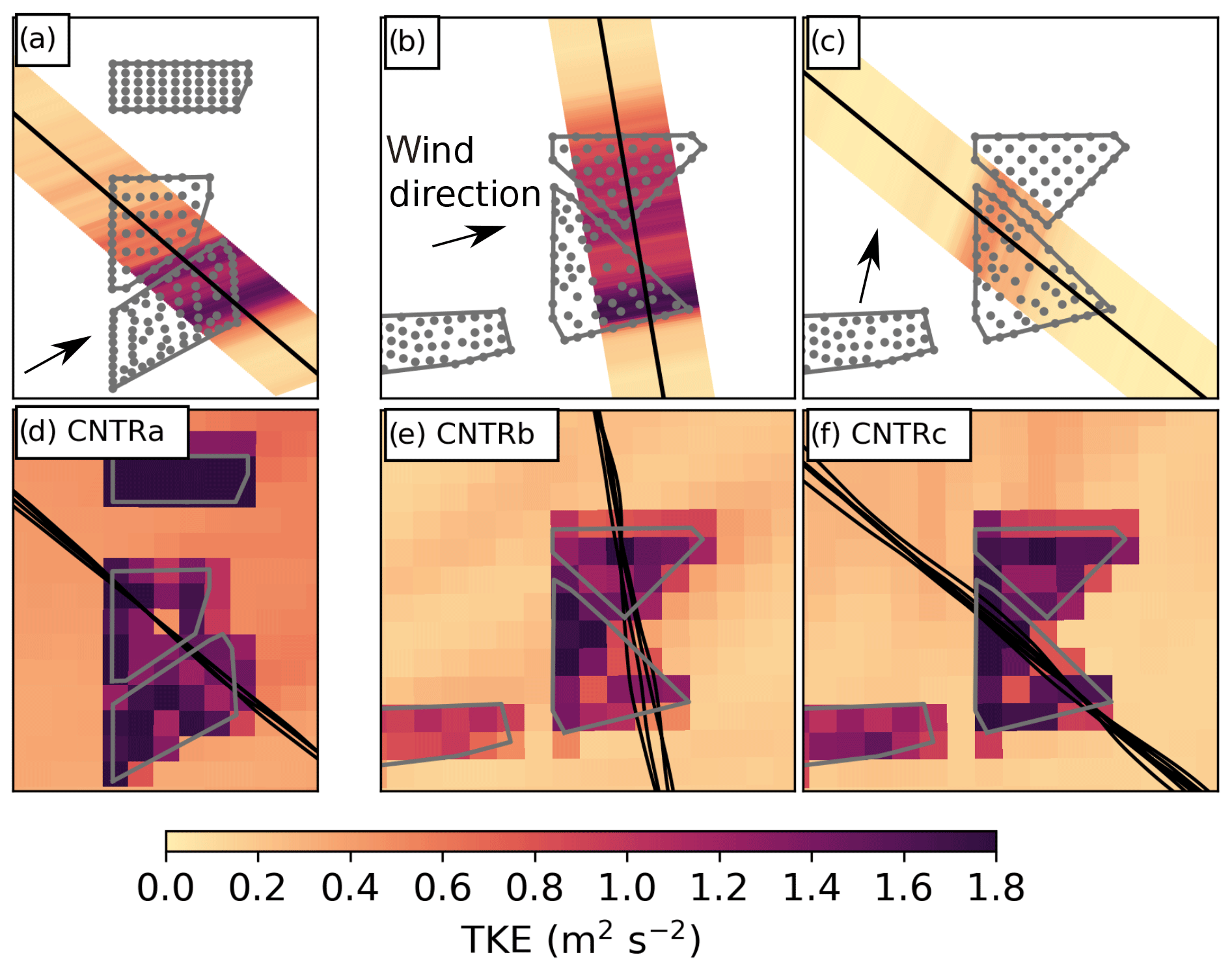
Figure 2The number of wind turbines within one grid cell in colored contours for the wind farms: (a) Meerwind Süd Ost (MSO) and OWP Nordsee Ost (ONO) and (b–c) Godewind Wind 1, 2 (GW) for the control simulations (CNTRa, CNTRb, CNTRc). The size of the contour areas corresponds to the size of the horizontal model grid. The circles denote the exact locations of the single wind turbines, whereby the wind turbines are colored according to the wind farm they belong to in panels (d)–(f); additionally, panels (e)–(f) show the horizontal grid with 5 and 16 km resolution for the following sensitivity studies: DX5, DX16, DX5noTKEsource and DX16noTKEsource (see Table 2 for an overview of all simulations). The wind turbines are not colored in panels (a)–(c) for better visibility of the wind turbine density. The gray lines denote the flight track of the research aircraft.
We conducted three control simulations, namely CNTRa, CNTRb and CNTRc, corresponding to the three case studies. These three simulations are identical in terms of their numerical setup; they only simulate different days.
All simulations were initialized the night before the observations at 00:00 UTC, resulting in a spin-up time of more than 12 h for case studies I and II, as suggested by Hahmann et al. (2015). Case study III took place earlier; hence, we originally started the simulations on 14 October 12:00 UTC. However, we obtained better results initializing the mode at 00:00 UTC the night before, resulting in a spin-up time of less than 12 h.
We use two different sets of vertical levels. The default configuration corresponds to that of Siedersleben et al. (2018a, b) with a vertical spacing of 35 m in the lowest 200 m and increasing to 100 m at 1000 m above mean sea level (a.m.s.l.), corresponding to one vertical level below the rotor area and three within the rotor area for the wind turbine type installed at the MSO and ONO wind farms (case study I; Fig. 3). Four vertical levels are located within the rotor area for the GW wind farm (Fig. 3) due to the larger rotor area. Lee and Lundquist (2017) obtained best results with 80 vertical levels – equal to a vertical spacing of 12 m below 400 m a.m.s.l. Therefore, we tested the sensitivity of our results using the vertical levels of Lee and Lundquist (2017) – equal to three full levels below and 10 full levels within the rotor area for the MSO and ONO wind farms (case study I) and two full levels and 13 full levels within the rotor area for the GW 1 and 2 wind farms (case studies I and II; Fig. 3).
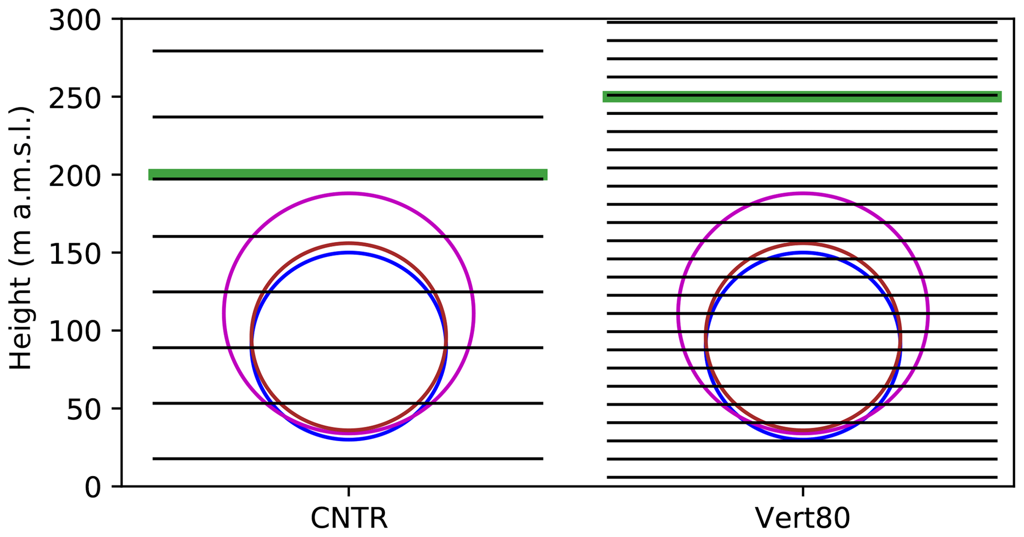
Figure 3Distribution of the vertical levels with height and the levels intersecting with the rotor areas of the two wind turbine types used in the wind farms, as listed in Table 3 for the CNTR and Vert80 simulations. The rotor areas of the wind turbines SIEMENS-SWT-6.0-154, SIEMENS SWT 3.6-120 and SENVION 6.2 are shown in magenta, blue and red, respectively. The green lines denote flight heights at 200 and 250 m a.m.s.l., which is necessary due to the different wind turbine heights.
We use the WFP of Fitch et al. (2012) to represent the wind farms in WRF. The parameterization extracts kinetic energy from the mean flow and adds TKE at the vertical levels intersecting with the rotor area, depending on the thrust and power coefficients of the wind turbines. The thrust coefficient describes the fraction of energy extracted from the mean flow in the parameterization of Fitch et al. (2012) (see Eq. 2 in Fitch et al., 2012); the power coefficient is the fraction of energy converted into electrical energy. These coefficients depend on the wind speed and wind turbine type because different wind turbine types are designed for different wind regimes.
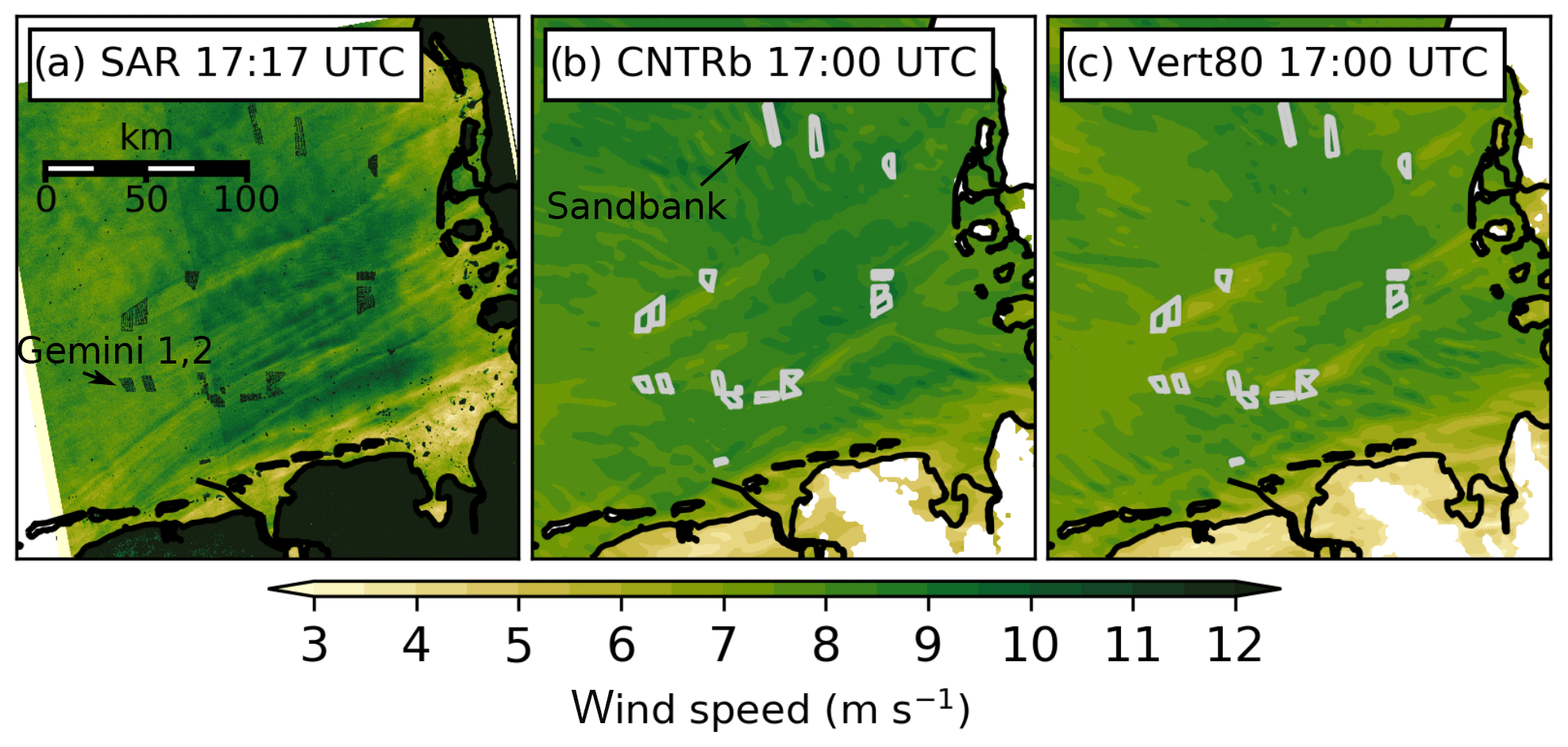
Figure 4A comparison of SAR from Copernicus Sentinel-1A and WRF retrieved wind speed at 17:17 and 17:00 UTC, respectively, on 14 October 2017 (case study II). The SAR data show the wind speed at 10 m, whereas the model output is taken from the model level closest to 10 m. Therefore, we show the wind speed at 17 and 15 m for the CNTR and Vert80 simulations, respectively. The grayish polygons (b–c) denote the locations of the wind farms.
The WFP of Fitch et al. (2012) neglects electrical and mechanical losses and assumes that all non-productive drag is converted into TKE. Consequently, the difference between the thrust and power coefficients describes the fraction of energy that is converted into TKE. More specifically, the amount of TKE added to the model is
whereby CT and CP are the thrust and power coefficients, and CTKE is the fraction of energy converted into TKE. Equation (1) is formulated for a Cartesian coordinate system with indexes i, j and k corresponding to directions x, y and z, that in turn are equal to the geographic directions west–east, south–north and the vertical axis with k=0 the level closest to the ground. The variable Nij describes wind turbine density within a grid cell i,j; Vijk is the horizontal wind speed at a grid cell ijk, intersecting with the rotor area, whereby VH is the wind speed at hub height at grid cell ij. (Redfern et al., 2019 showed that during strong shear events rotor-equivalent wind speed result in a different change in TKE.) Aijk is the rotor area between the two vertical levels k and k+1, at a height zk and zk+1. Consequently, the increase in TKE with time is highest for high wind speeds at the rotor area, high number of wind turbines in one grid cell and a large difference between the power and the thrust coefficient.
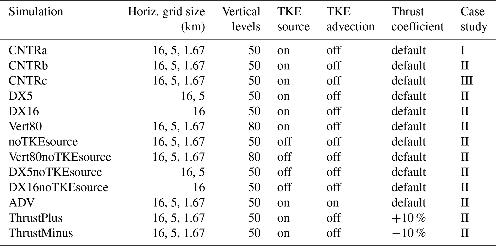
A summary of the setups of our sensitivity tests appears in Table 2. The sensitivity of our results with respect to the horizontal grid size was tested with simulations of 5 and 16 km horizontal resolution, respectively. Consequently, the number of turbines within one grid cell changes (Fig. 2). In Siedersleben et al. (2018a, b), we obtained best results using a horizontal grid size of 1.67 km.
The two sets of vertical levels demand two different time step configurations. For the default configuration, we use a time step of 60 s in the outermost domain, 20 s in the second domain and 5 s in the third domain. For the simulations using refined vertical levels, smaller time steps are necessary due to the higher resolution. Therefore, we use 10, 3.33 and 0.67 s, corresponding to the three domains. We named the simulations using 80 vertical levels Vert80.
Recently, some published studies (e.g., Abkar and Porté-Agel, 2015; Eriksson et al., 2015; Vanderwende et al., 2016; Pan and Archer, 2018) suggested that the mixing induced by the WFP of Fitch et al. (2012) is too high due to the added TKE into the model (see Eq. 1). Therefore, we tested the sensitivity of our simulations by switching the TKE source off. Three simulations were performed using a horizontal grid spacing of 1.67, 5 and 16 km with a disabled TKE source (noTKEsource, DX5noTKEsource, DX16noTKEsource). As we expect a simulation with more vertical levels to resolve more vertical shear, we additionally performed a simulation using 80 vertical levels with a grid size of 1.67 km and no TKE source (Vert80noTKEsource).
Starting from WRF version 3.5.0, TKE advection can be activated in the boundary scheme of Nakanishi and Niino (2006) (see Eq. 1.4 in Skamarock et al., 2008). In previously published studies (e.g., Mangara et al., 2019), this option was used. Therefore, we tested the sensitivity of our results with respect to this option. A summary of all sensitivity tests is shown in Table 2.
Public information on turbine thrust and power coefficients is not widely available, and so we also explored the sensitivity of our results to these parameters. We altered the estimated thrust coefficient similar to Siedersleben et al. (2018b) by ±10 %, resulting in two simulations (ThrustMinus, ThrustPlus) that are expected to introduce more and less TKE into the model than the CNTRb simulation. The results are presented in Sect. 5.4.
The following parameterizations were used: the WRF double-moment six-class cloud microphysics scheme (WDMS; Lim and Hong, 2010), the Rapid Radiative Transfer Model for GCMs (RRTMG) scheme for short- and longwave radiation (Iacono et al., 2008), the Noah land surface model (Chen and Dudhia, 2001) and the Mellor–Yamada–Nakanishi–Niino (MYNN) boundary layer parameterization (Nakanishi and Niino, 2006) interacting with the WFP of Fitch et al. (2012). Only the first domain uses the cumulus parameterization of Kain (2004) as the two innermost domains have a convection-permitting resolution.
Table 2Overview of performed numerical simulations and parameter choices for the sensitivity experiments.
2.4 Wind farms at measurement sites and in the mesoscale model
We conducted the three measurements at two different sites. Case study I took place at the wind farms Meerwind Süd Ost (MSO) and OWP Nordsee Ost (ONO) (Fig. 2a, d), whereas the other two case studies focus on Godewind 1 and 2 (GW) (Fig. 2b, c).
The wind farms MSO and ONO are equipped with SIEMENS SWT-3.6-120 and SENVION 6.2 turbines having a hub height of 90 and ≈95–97 m, respectively; a rotor diameter of 120 m, resulting in a rotor top of 150 and 157.4 m at most. GW wind farms are equipped with Siemens SIEMENS SWT-6.0-154 wind turbines that have a hub height of 110 m and diameter of 154 m, resulting in a rotor top of 187 m. Further details are provided in Table 3.
Table 3Wind turbine types installed at the measurement sites according to the data of the Bundesnetzagentur (2019).
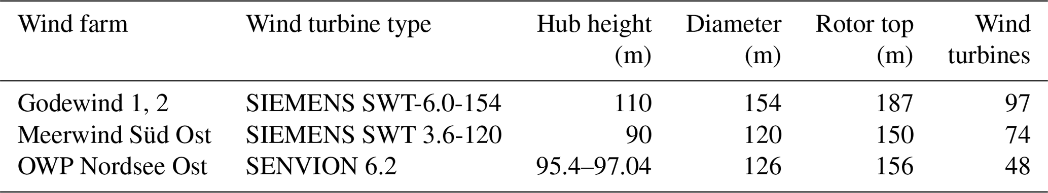
In this study, we use, as in Siedersleben et al. (2018b), the thrust and power coefficients of the wind turbine SWT 3.6-120-onshore, as these are freely available online (http://www.wind-turbine-models.com/turbines/646-siemens-swt-3.6-120-onshore, last access: 16 January 2018). We use these power and thrust coefficients for all wind turbines implemented in the model. However, the hub height and the rotor diameter were adapted for each wind turbine type in the simulations. The locations of the installed wind turbines (i.e., all blue wind turbines in Fig. 1) were taken from Bundesnetzagentur (2019).
According to the energy charts provided by Fraunhofer ISE (2019), all wind farms of interest were fully operational during the aircraft observations. Therefore, we used all wind turbines of the wind farms as given in Bundesnetzagentur (2019).
Here, we use ERA5 data to provide overviews of the synoptic situations before and during each case study (Copernicus Climate Change Service, C3S, 2018). Additionally, the vertical structure of the atmosphere is discussed by the use of the climb flight data. Finally, the results of the aircraft measurements over the wind farms for the three case studies are described in Sect. 3.2 and 3.3.
3.1 Synoptics and mesoscale overview based on ERA5 reanalysis, SAR and aircraft data
Case study I was slightly stably stratified with wind from the southwest (Fig. 6a, g). On 9 August 2017 at 15:00 UTC, a trough approached the German Bight from the north (Fig. 5a) associated with southwesterly winds of 10–12 m s−1 at hub height near MSO (Fig. 6d, g). Weak warm air advection was associated with a slightly stably stratified atmosphere according to the climb flight (Fig. 6g, anticyclonic turning of the wind with height) upwind of the wind farm cluster (for location of climb flight, see Fig. 1, black thick line). Despite the stably stratified atmosphere, the sea surface temperature (SST) was higher than the air temperature close to the surface. At the FINO1 tower, a SST of 292 K was measured, ≈2 K higher than the air temperature. As expected for summertime, the SST was highest closest to the coast (Fig. 5a).
Case study II was also stably stratified, with stronger winds from the west. On 14 October 2017 at 15:00 UTC, a deep trough located over the Atlantic caused a zonal jet over the North Sea (Fig. 5b) associated with wind speeds of up to 15 m s−1 at hub height (Fig. 6e) at the location of the climb flight (Fig. 1, green thick line). Due to the stably stratified atmosphere, the wind profile was characterized by strong vertical shear between 30 and 190 m a.m.s.l. (Fig. 6e), corresponding to the rotor area limits of the wind farm. According to the SAR data, the stably stratified atmosphere was associated with wakes longer than 50 km (Fig. 4a). Long wakes are visible downwind of the wind farms located near the German and Netherlands coasts. Further to the north, around the Sandbank wind farm (see annotation in Fig. 4a), only subtle wakes are visible, indicating less favorable conditions for wakes. However, Sandbank has only two turbine rows; hence, we expect generally weaker wakes during westerly winds at the Sandbank wind farm.
Case study III also experienced a stably stratified flow with 10 m s−1 wind speed and southerly wind direction (Fig. 6c, f, i). On 15 October 2017 (case study III), the trough over the Atlantic moved further to the west, causing a southwesterly warm air advection, that in turn resulted in a pronounced inversion with a temperature difference of 4 K between 30 and 190 m a.m.s.l. according to the profile recorded by the aircraft (Fig. 6c, magenta thick line in Fig. 1). Associated with the top of the inversion is a wind speed maximum at ≈190 m a.m.s.l. (Fig. 6f). From previous literature (e.g., Smedman et al., 1997; Dörenkämper et al., 2015; Svensson et al., 2016), we would expect a SST lower than the air temperature close to the sea surface. However, a SST of 288.5 K was measured at FINO1, in contrast to a potential air temperature of 285 K at 50 m a.m.s.l., according to the airborne measurements, indicating that the SST was higher than the air temperature. The two additional vertical profiles taken before and after the additional flyovers revealed a destabilization of the atmosphere (Fig. 6c).
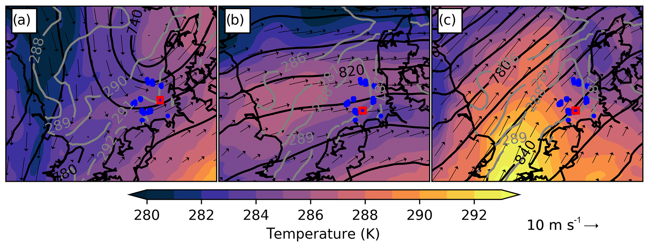
Figure 5ERA5 reanalysis data: temperature (colored contours; K) and geopotential height (20 m increments) as black contour lines at 925 hPa for the three case studies as listed in Table 1, at 15:00 UTC on 9 August 2017, at 15:00 UTC on 14 October 2017 and at 09:00 UTC on 15 October 2017 (Table 1). The gray solid contour lines show the SST.
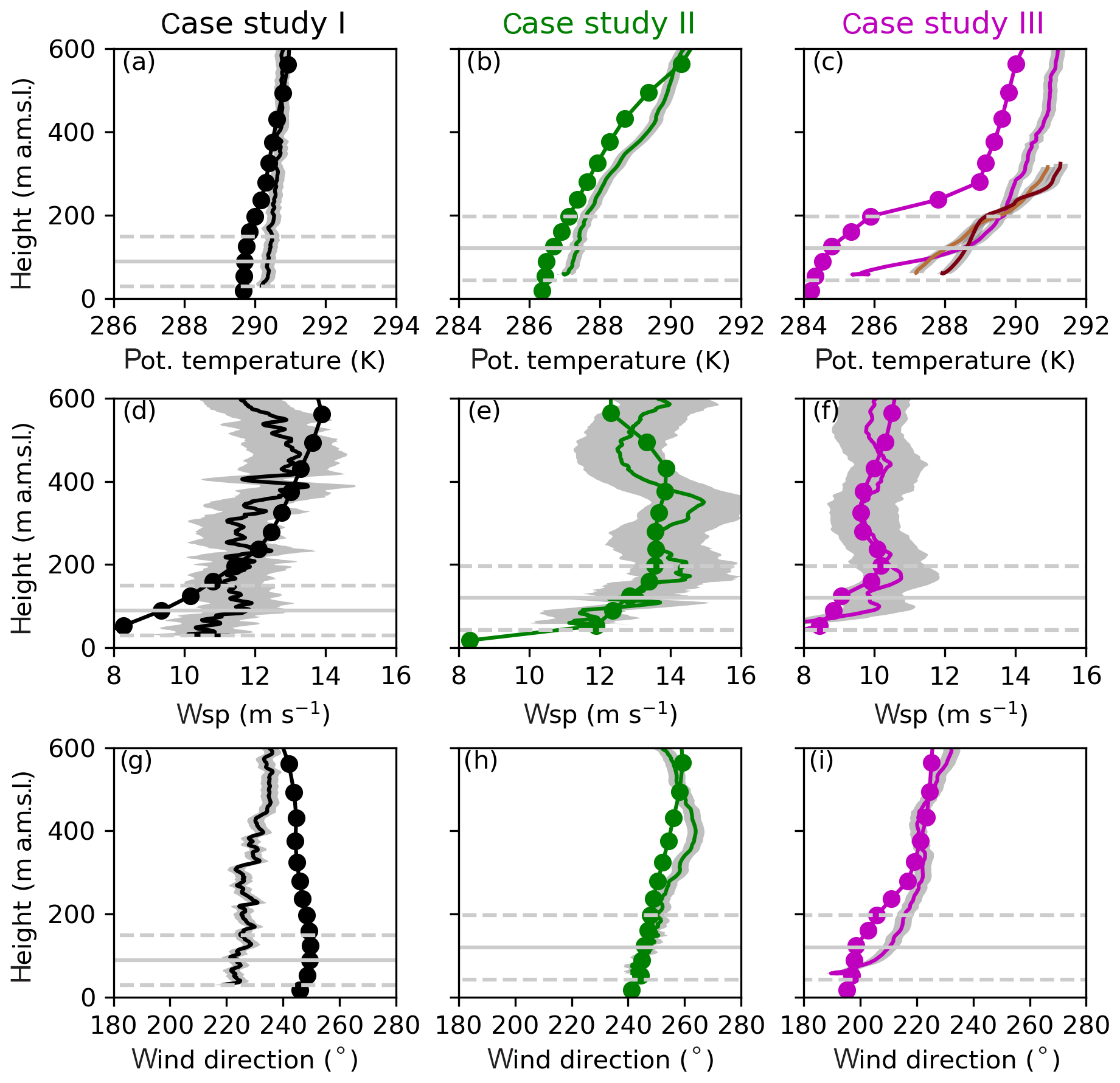
Figure 6Vertical profiles of potential temperature (a–c), wind speed (d–f) and wind direction (g–i) obtained by probing the atmosphere with the research aircraft (solid lines). The interpolated WRF data along the climb flight are shown with the line having the circles on top, whereby each circle represents a vertical level of the WRF control simulation (CNTRa, CNTRb, CNTRc). The gray shadings represent the error bars of the measurements. The dashed and solid gray lines denote the rotor area and the hub height of the wind turbines. As the measurements were conducted at two sites with two different wind turbine types, the heights of the hub and rotor areas vary. In panel (c), two additional vertical profiles are shown (red and light red) that were taken before and after the additional flyovers in case study III; for further details, see the text. Each column corresponds to one case study; i.e., the (a, d, g) column corresponds to case study I, similar to the coloring of flight tracks in Fig. 1.
3.2 Wind speed above and next to the wind farms
For case study I, wind speeds on the order of 13 m s−1 were observed at 200 m a.m.s.l. near the wind farms (Figs. 7a, 8a). During the four flights above the wind farms, the wind speed varied only by ± 0.5 m s−1, indicating that the weather situation was stationary. However, the variability of the wind speed measurements increases over the northern edge of the ONO wind farm. At the downwind side of the wind farm, the wind speed decreased in each observation by more than 1 m s−1, indicating that the wake of the wind farm extended to a height of 200 m. As the aircraft approached the upwind side of the wind farm (i.e., at 54.46∘ N latitude), the wind speed deficit decreased.
During case study II, the distinct wind farm wake was also accompanied by a speed-up around the farm, such as indicated by Nygaard and Hansen (2016). We observed a horizontal wind speed of ≈15 m s−1 at 250 m a.m.s.l. south of GW and slightly lower winds speeds to the north (Figs. 8b, 9b). At the southern edge of the wind farm, oriented parallel to the large-scale synoptic forcing, the wind speed dropped consistently in all four flight legs by up to 2 m s−1, associated with a speed up further south (see annotation of Fig. 8b). We suggest that this acceleration emerges due to an enhanced flow around the wind farm due to the stably stratified atmosphere. This stability hinders the flow to extend vertically above the wind farm and forces it to flow around the wind farm leading to a speed-up at the wind farm edges. Similar to case study I, the wind speed showed low variability during the measurements that were performed within a time interval of 50 min; highest variability occurred over the wind farms.
In comparison to case studies I and II, in III, the wind speed was barely influenced by the GW wind farms during the first flight legs. We suggest that this phenomenon is rooted in the strong inversion between 40 and 180 m a.m.s.l., decoupling the layer over the inversion from the surface layer. Consequently, the wind speed measurements showed only weak enhanced variability over the wind farms. However, two additional measurements were taken 40 min later. These two flyovers both show an enhanced deceleration over the wind farms, especially the last flight leg (purple line, Fig. 8c). The mean (shown in Fig. 8c) was calculated using only the first four flight legs.
3.3 TKE above and next to the wind farms
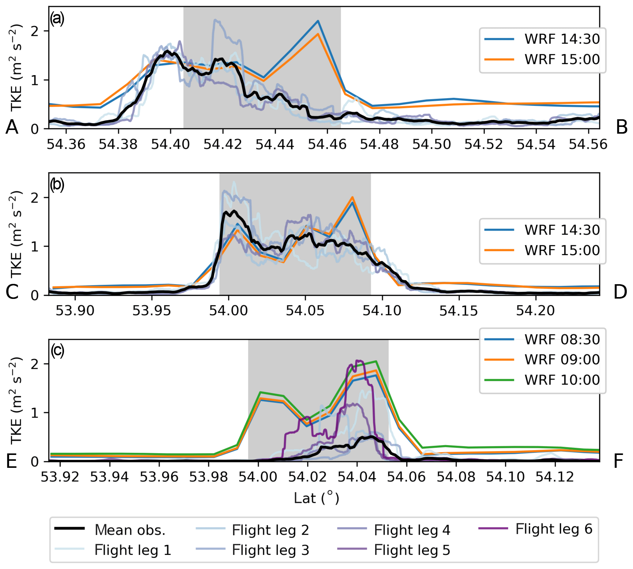
In case study I, the observed TKE above the wind farm was a factor of 10 higher than in the ambient flow. The TKE above the MSO and ONO wind farms was increased compared to the surroundings (Figs. 9a, 10a). More specifically, the research aircraft measured a TKE of up to 2.0 m2 s−2 but 0.2 m2 s−2 within the undisturbed environment, meaning that the TKE above the wind farms is almost 10 times higher, 50 m over the rotor top compared to the surrounding environment. This pattern was observed during all four flyovers (Fig. 10a). The mean of all measurements clearly indicates that the highest TKE was observed in the wake region of the MSO wind farm where the shear was largest (shown in Fig. 8a).
In case study II, TKE above the wind farms was a factor of 20 higher than that in the ambient flow. A TKE of up to 2.5 m2 s−2 was observed at 250 m a.m.s.l. above the GW wind farms and 0.1 m2 s−2 within the background flow (Fig. 9b). The TKE maximum, visible in all four flights (Fig. 10b), corresponds to the southern edge of the GW wind farms – the region with the highest horizontal wind shear (Fig. 8b). In contrast, no TKE maximum can be observed upwind at the northern edge of the GW wind farms.
In case study III, a strong inversion generated a stably stratified environment, resulting in the lowest TKE values observed within our three case studies in the background flow and above the wind farm (Figs. 9c and 10c). Nevertheless, the values of TKE above the wind farms during all six flights were elevated compared to surroundings. The TKE maximum matched in location with the western edge of the wind farm where the horizontal wind shear was largest (Fig. 8c) due to the southwesterly background flow. During the last flight leg, the aircraft observed TKE on the order of 1.6 m2 s−2, 3 times higher than in the measurements conducted 40 min before (Fig. 10c). This specific flight leg also showed the strongest wind deceleration above the wind farm (Fig. 8c).
In summary, in every case, above the wind farm, the aircraft observed values of TKE between 5 and 20 times larger than the ambient values of TKE.
Herein, we present control simulations for each of the three case studies (I, II and III). We start with a comparison of the vertical profiles of the aircraft measurements and the profiles obtained by the simulations. As we want to evaluate the TKE above the wind farms that is in turn highly dependent on wind shear, we compare the wind speed measurements with simulations before we evaluate the simulated TKE in Sect. 4.3.
4.1 Evaluation of the background flow
For case study I, the simulated potential temperature profile and the observations show a weakly stratified atmosphere (Fig. 6a), whereas the model is more stably stratified between 90 and 250 m a.m.s.l., resulting in stronger vertical wind shear in the model (Fig. 6d). This deviation could be rooted in a dislocation of the incoming trough, causing more westerly winds in the simulations than in the observations.
For case study II, the observed and simulated vertical structure of the atmosphere agree except for a cold bias in the potential temperature. The model predicts a potential temperature profile with a lapse rate similar to the observed one but with a cold bias of 0.5 K. The strong vertical wind shear within the lower rotor area is well represented, and so is the wind direction. Consequently, the orientation of the wakes in the SAR satellite observations (Fig. 4a) matches with that of the simulated wakes in Fig. 4b). Note that the SAR image taken on 14 October 2017 at 17:17 UTC should be only used to evaluate the orientation of the wakes. The lowest level of the control simulation is at 17 m a.m.s.l. Consequently, interpolating the wind speed to a height of 10 m is difficult. Therefore, we show the simulated wind speed at 17 m in Fig. 4b) for simplicity.
For case study III, the simulations show a less pronounced inversion than the observations (Fig. 6c). This behavior of the model is similar to the case study presented in Siedersleben et al. (2018b), where an inversion similar to the one shown in Fig. 6c) developed and the WRF model also had problems representing the inversion. In this case, the inversion is even more pronounced, most likely associated with the proximity of the vertical profile to the coast (Fig. 1, thick magenta line), increasing the challenge for the model to capture the heterogeneity. However, this inversion weakened during the observation but the stratification of the atmosphere in the model did not change over time. Therefore, the simulated profiles before and after additional flights are not shown in Fig. 6c.
4.2 Impact of wind farm parameterization on wind speed above wind farm
The simulation for case study I generally underestimates the wind speed at 200 m a.m.s.l. above and next to the wind farms by up to 2 m s−1 (Figs. 7a, 8a). The sharp decrease of 1 m s−1 within the wake is captured by the model at 15:00 UTC but not at the beginning of the measurements at 14:30 UTC. A weak increase in wind speed similar to the observation is represented over the wind farm (i.e., within the gray shaded area in Fig. 8a), associated with the shorter distance of the upwind edge of the wind farm. A possible explanation for the wind speed bias between model and observation could be a more unstably stratified atmosphere in the simulations. However, the model adequately represented the stratification of the atmosphere in the vicinity of the wind farms (Fig. 6a). Therefore, we suggest that the atmosphere was more stably stratified to the west during the observation than in the simulations.

Figure 7Plan view on observed (a–c) and simulated (d–f) horizontal wind speed at 14:30, 15:00 and 09:00 UTC on 9 August, 14 and 15 October 2017, respectively, with horizontal wind speed in colored contours at 200 (a, d) and 250 m a.m.s.l. (b, c, e, f). Black lines denote the flight path over the wind farms. The observations show the mean of the observed wind speed, similar to Fig. 8a–c. The locations of wind farms and single wind turbines are shown in gray polygons and dots, respectively. Each column corresponds to one case study (e.g., panels a and d correspond to the measurements taken on 9 August 2017). The wind direction is denoted by the black arrow as retrieved by the aircraft observations.
The simulations for case study II represent the stationary background flow (i.e., no variance between 14:30 and 15:00 UTC) and the impact of the GW wind farms well. The averaged wind speed matches with the simulated wind speed within ±0.2 m s−1, except at the southern edge of the wind farm – there, the horizontal wind speed gradient is more pronounced in the observations than in the simulations. However, this deviation is likely rooted in the rather coarse horizontal grid size of the model.
The model underestimates the wind speed compared to the measurements conducted during case study III. Over the wind farms, the deviations between simulations and observations are largest for the first four flyovers, indicating a more pronounced impact of the wind farms on the atmosphere in the simulations than in the observations. However, at 10:00 UTC, the observation showed a more pronounced decreased wind speed over the wind farms, similar to simulations, with a constant negative bias of ≈2.0 m s−1.
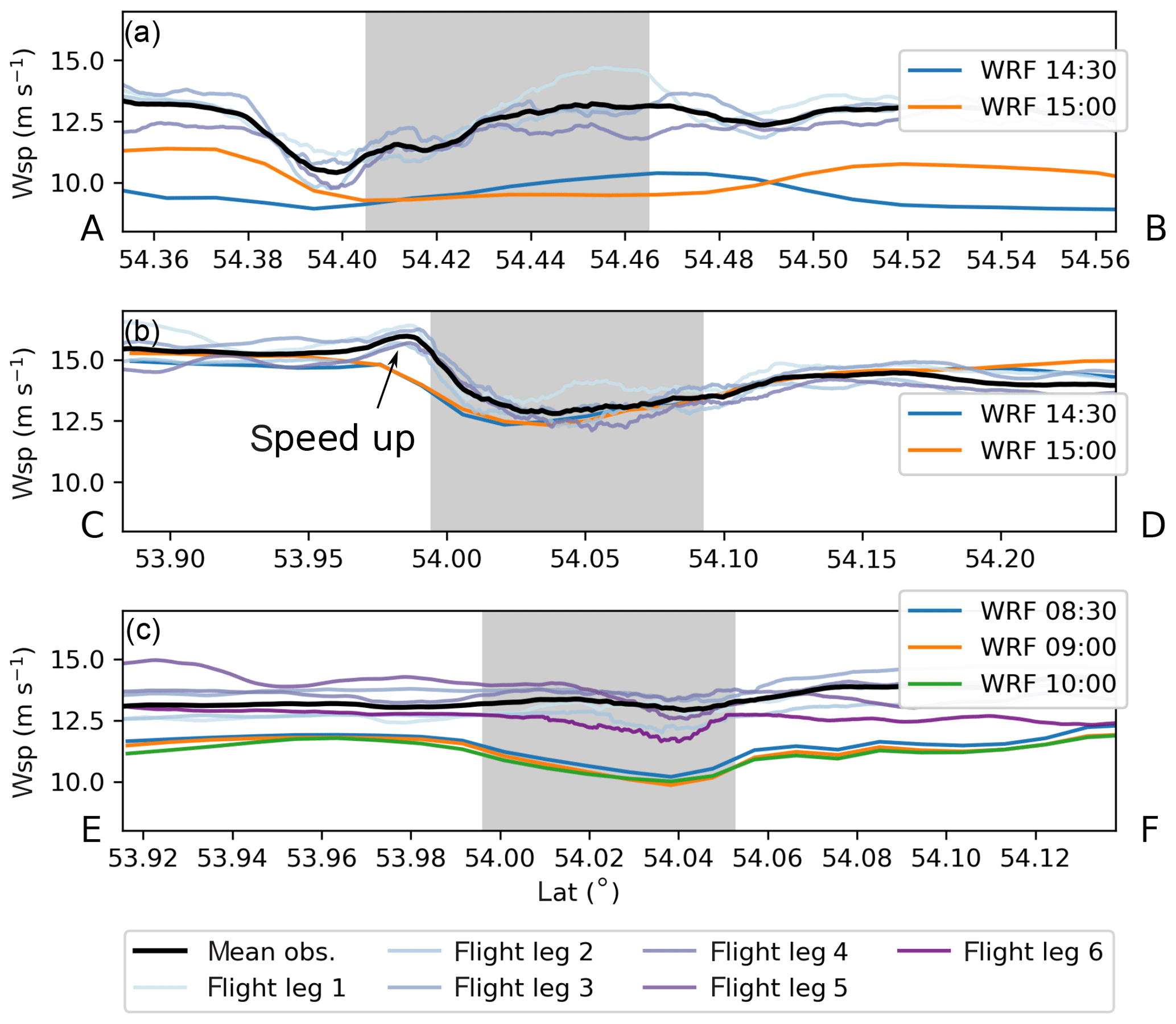
Figure 8Observed (thin blue and purplish lines; the purple amount is increased based on how late the flight leg was flown) and simulated wind speed interpolated onto the flight track, as shown in Figs. 1 and 2 for the three case studies (a–c) as indicated in Table 1. Note the mean speed is more or less perpendicular to the flight legs (see Fig. 7a, b, c); hence, the mean wind speed points into the paper plane. The thick black line shows the mean of all wind speed measurements over the wind farms similar to the measurements shown in Fig. 7a–c. The gray shaded areas denote the location of the wind farm. The capital letters on the x axis show the orientation of the axis as indicated in Fig. 1.
4.3 Impact of wind farm parameterization on TKE above wind farms
The increased TKE over the wind farms is captured by the simulations but not the shape of the TKE profile over the wind farms. For example, in case study I, the WFP simulates a TKE over the wind farms with two peaks (Figs. 9a, 10a), whereby the first peak matches with the observed TKE maximum with ≈1.5 m2 s−2. However, this peak in TKE corresponds in the observations to the southern edge of the wake that developed behind the farm, whereas in the simulations this peak corresponds to the southern edge of the wind farm (Fig. 2a). The second peak at 54.46∘ N in simulations with a TKE of 2.0 m2 s−2 corresponding to the upwind side of the wind farm was not observed.
A similar pattern can be observed for the simulations of 14 October 2017. The TKE maximum at the southern edge of the wind farms is captured by the model (Figs. 9b, 10b). In contrast, the declining trend of TKE towards the northern edge of the wind farm is interrupted in the model. The TKE of the undisturbed flow next to the wind farm is very similar to the observed TKE, increasing the confidence in this simulation.
In contrast to the other case studies, in case study III, the TKE in the observations evolves over time. Initially, the simulated TKE is more than twice as high as the averaged observed TKE over the wind farms: 1.0 m2 s−2 for the first four flyovers compared to 2.0 m2 s−2 (Figs. 9c, 10c). However, 40 min later, the measured TKE from the additional two flight legs shows a value similar to the simulations. Especially the last flight leg shows a TKE of 2.0 m2 s−2 at the western edge of the wind farm. This flight leg also has the most pronounced wind speed deficit over the wind farm, agreeing best with simulated impact on the horizontal wind speed at 250 m a.m.s.l.
In case study II, the model captures the background flow providing a sound basis for sensitivity studies. In contrast, the simulations for case studies I and III both have a bias in the wind speed at 200 m or 250 m over and next to the wind farms associated with a deviation considering the intensity of an inversion for case study III. For case study I, we can only suggest that the negative bias in the horizontal wind speed is rooted in the stratification of the model due to the lack of measurements available at the North Sea.
Given the success with the simulation CNTRb – case study II, we explore the sensitivity of the WFP of Fitch et al. (2012) with respect to horizontal grid size, the TKE source, vertical resolution, TKE advection and thrust coefficient in Sect. 5.1, 5.2, 5.3 and 5.4.
5.1 Sensitivity to horizontal and vertical resolution with an active TKE source
We conducted two additional simulations with a horizontal grid size of 5 and 16 km with the TKE source of the WFP of Fitch et al. (2012) activated; these simulations are called DX5 and DX16. Additionally, a third simulation was performed with the same configuration as CNTRb but with 80 vertical levels (Vert80). A summary of all sensitivity tests is given in Table 2.
Coarsening the horizontal resolution of the simulations to 5 km resolution degrades the agreement between the simulations and observations (Figs. 11, 12b). As expected, the sharp drop in the horizontal wind speed in the observations at the southern edge of the wind farm oriented parallel to the incoming flow cannot be represented in a mesoscale simulation with a horizontal grid size of 5 km, a result similar to the CNTRb simulation (Fig. 11b). However, the wake impact on the horizontal wind speed at 200 m a.m.s.l. (i.e., 60 m above the wind farms) is captured well, rooted in a TKE only 0.3 m2 s−2 lower than the observed mean (Figs. 11a, 12b), except for the region of strong horizontal shear (Fig. 13b) that cannot be captured by a mesoscale model.
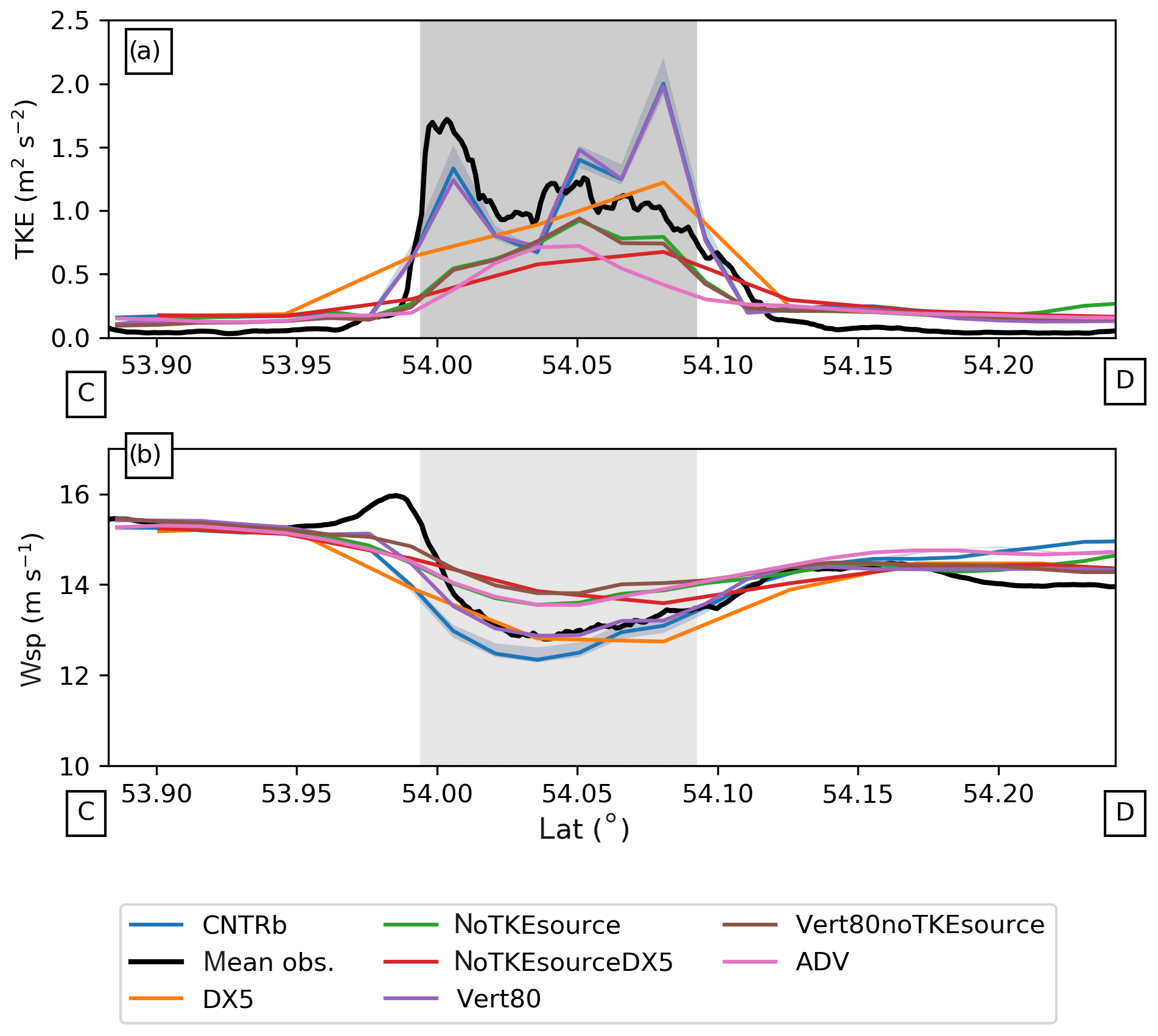
Figure 11As in Fig. 8 but for TKE (a) and wind speed (b) for the sensitivity simulations DX5, noTKEsource, DX5noTKEsource, Vert80, Vert80noTKEsource and ADV conducted for case study II at 15:00 UTC. A summary of all sensitivity tests is listed in Table 2. For better comparison, the control simulation CNTRb is plotted as well.
Simulation DX16 reveals that a grid size of 16 km cannot capture the effect of wind farms with a size on the order of 100 km2 by the use of a WFP. Compared to CNTRb, the decrease in wind speed downwind of the GW wind farms is on the order of 1 m s−1 instead of 2 m s−1, suggesting that the vertical mixing is underestimated. Accordingly, Fig. 12c reveals that the simulated TKE is 2 times lower than observed.
More vertical levels cause the same amount of TKE over the wind farm compared to CNTRb (Figs. 11a, 12g), but the wind speed deficit at the southern edge of wind farm is in better agreement with the observations (Figs. 13g, 11b) by up to 0.5 m s−1. Additionally, the wakes as seen in the SAR image match better with the ones simulated in Vert80 than those in CNTRb (Fig. 4). The wakes in Vert80 (Fig. 4c) are more pronounced compared to those in CNTRb (Fig. 4b) and hence fit better to the observed SAR image.
5.2 Sensitivity to vertical resolution with a disabled TKE source
For comparison to wind farm parameterizations without an explicit turbulence source (e.g., Volker et al., 2015), we conducted three simulations with the TKE source of the Fitch et al. (2012) parameterization switched off using the CNTRb configuration and two coarser horizontal grids than in CNTRb (noTKEsource, DX5noTKEsource, DX16noTKEsource; Figs. 12d–f, 13d–f). Additionally, we performed a simulation having the TKE source disabled with 80 vertical levels, namely Vert80noTKEsource (Fig. 13h).
All simulations with the TKE source switched off show larger wind speeds over the wind farms. For example, in the simulation noTKEsource, wind speeds are ≈14 m s−1 above the wind farm (Fig. 13d) associated with a lower TKE (Fig. 11a) than in CNTRb. Consequently, we expected even higher wind speeds in DX5noTKEsource over the wind farms associated with the lower TKE that can be resolved in a simulation with a grid size of 5 km. Indeed, the wind speed and the TKE over the farms is up to 0.5 and 0.3 m2 s−2 lower than that in CNTRb (Fig. 13e). Obviously, simulation DX16noTKEsource fails in representing the impact of the wind farms on the wind speed (Fig. 13f) and the TKE (Fig. 12f).
Surprisingly, the simulation Vert80noTKEsource with 80 vertical levels shows approximately the same TKE as that simulated in noTKEsource with 50 vertical levels, although more vertical shear should be resolved in Vert80 (Fig. 11a). This amount of TKE is similar to the noTKEsource simulation. Consistently, the wind speed reduction over the wind farm is almost similar to the noTKEsource simulation (Fig. 13b).
Summarized, all simulations without a TKE source produced too-small amounts of TKE compared to the observations. Therefore, we conclude that additional TKE is necessary to parameterize wind farms in mesoscale models in stable conditions.
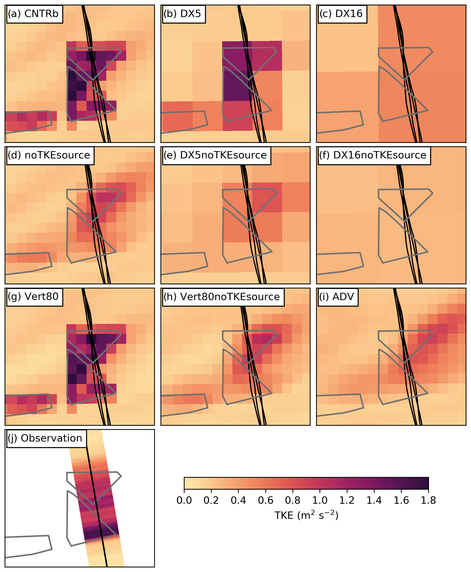
Figure 12As in Fig. 9 but for the sensitivity simulations (b–i) DX5, DX16, noTKEsource, DX5noTKEsource, DX16noTKEsource, Vert80, Vert80noTKEsource and ADV at 15:00 UTC. A summary of all sensitivity tests is listed in Table 2. For better comparison, the control simulation CNTRb is shown in panel (a) and the observations in (j).
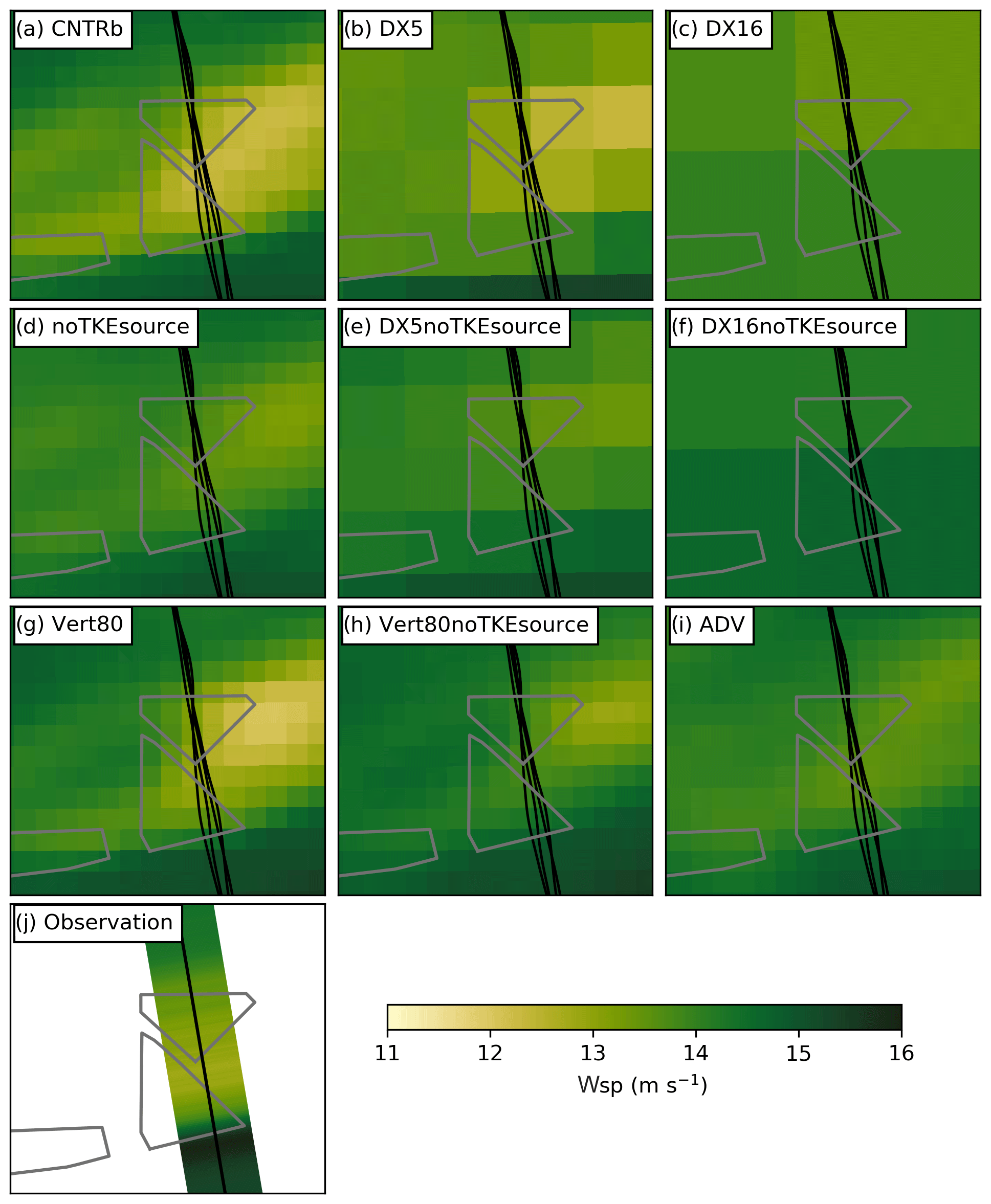
Figure 13As in Fig. 7 but for the sensitivity simulations (b–i) DX5, DX16, noTKEsource, DX5noTKEsource, DX16noTKEsource, Vert80, Vert80noTKEsource and ADV at 15:00 UTC. A summary of all sensitivity tests is listed in Table 2. For better comparison, the control simulation CNTRb is shown in panel (a) and the observations in (j).
5.3 Sensitivity to advection of TKE
The TKE advection option results in a largely reduced TKE over the wind farm associated with a lower wind speed reduction over the wind farm. The simulated TKE is almost the lowest parameterized in all simulations performed for this study (Fig. 11a), resulting in an underestimation of the wind farm impact on the wind speed over the wind farm of −2 m s−1 less than the observed mean deficit (Figs. 13i, 11b). However, the ADV (i.e., advection of TKE is active) simulation shows the highest TKE values within the wake of the GW wind farm (Fig. 12i). The simulated TKE within the wake is on the order of 0.6–0.8 m2 s−2, meaning that the simulated TKE in the wake is more than twice as high as that in the undisturbed flow. This finding is in contrast to the observations reported in Platis et al. (2018); they measured the lower TKE values within the wake than in the ambient flow during stable conditions. Summarized, although it is expected that the advection of TKE is supposed to improve generally mesoscale simulations with horizontal resolutions on the order of 1 km, we observed here two drawbacks with respect to the wind farm parameterization of Fitch et al. (2012). Firstly, the TKE above the wind farm was too low associated with too-high wind speeds above the wind farm. Secondly, according to airborne observations of Platis et al. (2018), the TKE within the wake is lower than that in the ambient flow and enhanced at the edges of wakes; in contrast, activating the TKE advection option results in an enhanced TKE within the wake. Therefore, we conclude not to use the TKE advection option for wake simulations during stable conditions at offshore sites.
5.4 Sensitivity to thrust coefficient
Two simulations (ThrustMinus, ThrustPlus) were performed to investigate the uncertainty introduced by the estimated thrust and power coefficients. The corresponding uncertainty is shown in Fig. 11 as shaded area around the results of the CNTRb simulation. The uncertainty in TKE due to the unknown power and thrust coefficients is smaller than the deviation caused by all sensitivity studies, except for simulation Vert80 (Fig. 11a). The uncertainty resulting for the wind speed deficit is smaller than the effect of all the other physics and numeric permutations tested here, including a change in the number of vertical levels (Fig. 11b).
Obviously, the most important ingredient for simulating realistic wind speeds over offshore wind farms is the correct representation of the atmospheric state, regardless in which configuration the WFP is used. In two of the three case studies examined here, the simulations analyzed here failed to represent the atmospheric background correctly. WRF captured the state of the atmosphere for case study II, as the boundary layer upwind of the GW wind farms was not modified by land. In contrast, the upwind conditions were not captured for case studies I and III. Both cases were characterized by a large-scale flow modified by the land upwind and stable conditions although the SST was higher than the air temperature. The model evaluation in Sect. 4.1 revealed that the associated inversion in case study III, that developed as warm air masses were advected from the land upwind over the German Bight, is challenging for the simulation, as described in Siedersleben et al. (2018b). The inversion almost decoupled the layer at 250 m from any processes below 200 m (i.e., top of inversion height), resulting in a very low signal of the wind farm in the TKE and wind speed (Figs. 9c, 10c). In contrast, the simulation showed TKE values up to 2.0 m2 s−2. However, during the additional two flyovers, the TKE increased up to 2.0 m2 s−2 in the observations associated with a destabilizing MABL as Fig. 6c) reveals. Consequently, the TKE over the wind farms increased, corresponding to an increased wind speed deficit during the last flyover. As the destabilization of the MABL resulted in a profile with a potential temperature gradient similar to the simulated profile, the simulated and observed TKE values have the same magnitude for the last two flyovers, underlining that the upwind conditions are crucial for representing the impact of offshore wind farms.
Based on the successful representation of case study II, we suggest that mesoscale wind farm simulations should use an additional TKE source during stable conditions, as the mixing and the associated wind deficit over the wind farms are too low otherwise.
Given the success with the TKE source switched on, we recommend for regional climate simulations using horizontal grids on the order of 5 km to use a WFP with an active TKE source. Additionally, the grid size must accommodate the size of the wind farms installed in the region of interest. For example, a regional climate simulation using a grid as Vautard et al. (2014); Miller and Keith (2018) (i.e., 50 and 30 km grids, respectively) would be unsuited for determining the climate impact of offshore wind farms on the German Bight, because we have shown that simulations with a horizontal grid size of 16 km are already too coarse to represent the impact on the MABL realistically. In contrast, simulations with a horizontal grid size of 5 km performed adequately when TKE was actively added to the model.
Strong shear lines that originate in the flow around the wind farm cannot be captured by mesoscale models. The strong horizontal shear, observed at the GW wind farm at the southern edge oriented parallel to the impinging flow, has a horizontal extent of ≈2 km. Following Skamarock (2004), realistic solutions only exist for processes having 7 times the grid size. Consequently, the horizontal shear with the associated TKE cannot be represented by mesoscale models. However, in the simulation for case study II, one could think that the model is able to present the shear line at the southern edge, when considering only the TKE. Both the simulation and the observation show a TKE maximum at the southern edge of the wind farm. However, the peak in the observations was associated with the horizontal wind shear. In the model, the GW wind farm extends more to the south than in reality; hence, the TKE peak in the simulations is associated with the TKE source of the WFP and not with the horizontal shear.
The WFP's TKE source possibly introduces too much TKE on the upwind edge of a wind farm. Although the simulations did not capture the atmospheric background in case study I, we noticed an important difference between the simulated and observed TKE. In the observations, the TKE over the wind farms increased as the flow penetrated through the wind farms (Fig. 10a), whereas the model added the most TKE at the upwind side of the wind farm. The amount of TKE added to the model depends on the wind speed, number of wind turbines and CTKE (see Eq. 1). Therefore, the added TKE is highest at the locations with the highest wind speeds within the farm, that is, at the front row of the wind farm. Of course, if the front row is associated with a high wind turbine density, the WFP also adds the most TKE at the upwind side of the wind farm. In case study I, wind turbine density is high, with up to five turbines per grid cell at the western edge of the wind farms (Fig. 2a). Additionally, we had southwesterly winds exposing the western edge of the wind farms to the highest wind speeds (Fig. 7a). Consequently, the simulated TKE has a maximum at the upwind side that was not observed in the aircraft measurements (Figs. 9a, 10a). However, without a TKE source, the deceleration was too low compared to the observations, especially when horizontal grids are larger than or equal to 5 km. The recommendations given here are based on one case study and might have to be adapted for wind farms of a different size.
The uncertainty of our simulations for case study II, introduced by the estimated thrust and power coefficients, is smaller than the effect of changing either the horizontal resolution or disabling the TKE source of the WFP of Fitch et al. (2012). Therefore, our sensitivity experiments conducted for case study II give useful and general recommendations for offshore wind farm simulations under stable conditions.
Using airborne measurements of wind speed and turbulent kinetic energy near offshore wind farms, we evaluate the wind speed and turbulent nature of the wind farm wakes as well as the parameterization of those wind farm wake effects enabled by the Weather Research and Forecasting Model (WRF) wind farm parameterization (WFP) of Fitch et al. (2012). Our study considered three cases at two different sites. Three case studies were all characterized by stable conditions. During two case studies, the marine boundary layer was highly influenced by the land upwind, resulting in deviations between observation and simulations. However, during one case study, the impinging flow was coming from the west, resulting in an inflow unaffected by any land. Hence, the WRF model represented the state of the atmosphere in the vicinity of the wind farms reasonably well. That allowed us to perform sensitivity studies in terms of horizontal and vertical resolution. Additionally, we investigated the effect of the TKE source of the WFP of Fitch et al. (2012) on the MABL as well as the option of advecting TKE in the boundary layer scheme of WRF. These are our main findings:
-
We recommend using the TKE source of the WFP of Fitch et al. (2012) for offshore wind farm simulations under stable conditions, especially for simulations having a horizontal grid coarser than or equal to 5 km. However, we notice that the WFP adds too much TKE at the upwind side of a wind farm. We observed during two case studies that the TKE over the wind farms increased with the path of the air through the wind farm, meaning that the TKE is higher at the downwind side of a wind farm than on the upwind side. In contrast, the WFP simulated the highest TKE at the upwind side of the wind farm associated with the highest wind speeds and wind farm density at the front row turbines. Nevertheless, the wind speed deficit is underestimated with disabled TKE source. Therefore, we suggest using the TKE source for stable conditions.
-
Simulations using the WFP of Fitch et al. (2012) using a grid size of ≈15 km or more underestimate the impact of wind farms on the MABL under stable conditions, regardless of the mode of the TKE source. Given the fact that the impact of offshore wind farms is largest during stable conditions, we suggest that climate simulations assessing the impact of offshore wind farms should use a horizontal grid on the order of 5 km or finer. This horizontal resolution is difficult to achieve for global simulations but feasible for regional climate and weather simulations.
-
In terms of the vertical resolution, we obtained best results with 80 vertical levels, equal to a spacing of 12 m below 400 m a.m.s.l. as in Lee and Lundquist (2017). We tested two sets of vertical levels, resulting in 3 (1) and 13 (4) levels below and within the rotor area. In the case of an activated TKE source, only minor differences were observed between the two sets of vertical levels. However, the wind speed deficit was captured better with the finer vertical resolution. Additionally, the simulated wakes agreed better with SAR data due to the smaller spacing of the vertical levels close to the surface. Therefore, we recommend a spacing of the vertical levels on the order of ≈12 m for offshore simulations. In the event that computational resources are limited, simulations with a horizontal and vertical resolution of 5 km and 35 m below 100 m also captured the most important features over the wind farms.
-
Activating the TKE advection in the boundary layer scheme was associated with too-low TKE over the wind farms that in turn resulted in an underestimation of the wind speed deficit over the wind farm.
These results support the hypothesis that the TKE source in the WFP of Fitch et al. (2012) is necessary under stable conditions at offshore wind farm sites, although we suggest that the added TKE is overestimated at the upwind side of the wind farms, suggesting possible future improvements. For comparison, it would be interesting to simulate case study II with the wind farm parameterization of Volker et al. (2015). Given the results of this study, previously published studies assessing the impact of offshore wind farms have possibly underestimated the impact on the marine boundary layer. Hence, we suggest regional climate simulations for offshore sites with a grid size of 5 km or finer. However, the skill of such regional climate simulations is lessened when flow is from onshore due to difficulty in parameterizing coastal effects. Thus, future work on wake effects of large offshore wind farms should primarily focus on boundary layer parameterizations that are able to capture the transition from land to open sea, and vice versa.
The WRF code is publicly available at http://www2.mmm.ucar.edu/wrf/users/downloads.html (National Center of Atmospheric Research, 2017). The WRF configuration files and the wind farm parameterization of Fitch et al. (2012) with the TKE source switched off are available on Zenodo (https://doi.org/10.5281/zenodo.3490732; Siedersleben et al., 2019).
The airborne data are available on PANGAEA (https://doi.org/10.1594/PANGAEA.902845; Bärfuss et al., 2019), whereby the data are described in detail in Lampert et al. (2019). The locations of the wind turbines are available at https://www.bundesnetzagentur.de (Bundesnetzagentur, 2019). The ERA5 data that were used for driving the WRF model can be downloaded via two Python scripts provided in the Zenodo repository (https://doi.org/10.5281/zenodo.3490732; Siedersleben et al., 2019).
SKS and JKL outlined the manuscript, and SKS wrote the manuscript with comments from JKL, AL, AP, BD, JSS, SE, JB and BC. BD drafted Sect. 2.2. SKS and AP performed the analysis of the simulations and the aircraft measurements, respectively. AL, KB, AP and JB executed the aircraft measurements. AP and JB designed the flight pattern over the wind farms. SE and JKL supervised SKS. The WIPAFF project was led by SE and TN.
The authors declare that there is no conflict of interest.
The views expressed in the article do not necessarily represent the views of the DOE or the U.S. Government.
Julie K. Lundquist's effort was supported by an APUP agreement with the National Renewable Energy Laboratory. Funding was provided by the US Department of Energy, Office of Energy Efficiency and Renewable Energy, Wind Energy Technologies Office.
The graduate school GRACE funded the research stay at CU of Simon K. Siedersleben. The WRF output was post-processed by the use of the Python library wrf-python (Ladwig, 2019) and visualized with Matplotlib (Hunter, 2007). The simulations were performed on the keal cluster hosted by IMK-IFU and gratefully managed by Benjamin Fersch. We would like to thank the aircraft crew (Rolf Hankers, Thomas Feuerle, Helmut Schulz and Mark Bitter) for conducting the flights. We visualized the WRF data by using colors, as suggested by Stauffer et al. (2015) and Thyng et al. (2016). We also thank the European Space Agency (ESA) for making Copernicus Sentinel-1 SAR data freely available.
The WIPAFF project is funded by the German Federal Ministry of Economic
Affairs and Energy (grant no. FKZ 0325783) on the basis of a decision by the German Bundestag. Funding provided by the U.S. Department of Energy Office of Energy Efficiency and Renewable Energy Wind Energy Technologies Office.
The article processing charges for this open-access
publication were covered by a Research
Centre of the Helmholtz Association.
This paper was edited by Simon Unterstrasser and reviewed by Tobias Ahsbahs and two anonymous referees.
Abkar, M. and Porté-Agel, F.: A new wind-farm parameterization for large-scale atmospheric models, J. Renew. Sustain. Ener., 7, 013121, https://doi.org/10.1063/1.4907600, 2015. a
Ahsbahs, T., Badger, M., Volker, P., Hansen, K. S., and Hasager, C. B.: Applications of satellite winds for the offshore wind farm site Anholt, Wind Energ. Sci., 3, 573–588, https://doi.org/10.5194/wes-3-573-2018, 2018. a
Bärfuss, K., Hankers, R., Bitter, M., Feuerle, T., Schulz, H., Rausch, T., Platis, A., Bange, J., and Lampert, A.: In-situ airborne measurements of atmospheric and sea surface parameters related to offshore wind parks in the German Bight, https://doi.org/10.1594/PANGAEA.902845, 2019. a
Bundesnetzagentur: Anlagenregister, available at: https://www.bundesnetzagentur.de/DE/Sachgebiete/ElektrizitaetundGas/Unternehmen_Institutionen/ErneuerbareEnergien/ZahlenDatenInformationen/EEG_Registerdaten, last access: 21 September 2019. a, b, c, d, e
Chen, F. and Dudhia, J.: Coupling an Advanced Land Surface-Hydrology Model with the Penn State-NCAR0 MM5 Modeling System. Part I: Model Implementation and Sensitivity, Mon. Weather Rev., 129, 569–585, https://doi.org/10.1175/1520-0493(2001)129<0569:CAALSH>2.0.CO;2, 2001. a
Christiansen, M. B. and Hasager, C. B.: Wake effects of large offshore wind farms identified from satellite SAR, Remote Sens. Environ., 98, 251–268, https://doi.org/10.1016/j.rse.2005.07.009, 2005. a
Copernicus Climate Change Service (C3S): ERA5 Fifth generation of ECMWF atmospheric reanalyses of the global climate, Copernicus Climate Change Service Climate Data Store, available at: https://cds.climate.copernicus.eu/cdsapp#!/home, last access: 14 November 2018. a, b
Corsmeier, U., Hankers, R., and Wieser, A.: Airborne turbulence measurements in the lower troposphere onboard the research aircraft Dornier 128-6, D-IBUF, Meteorol. Z., 10, 315–329, https://doi.org/10.1127/0941-2948/2001/0010-0315, 2001. a
Djath, B., Schulz-Stellenfleth, J., and Cañadillas, B.: Impact of atmospheric stability on X-band and C-band synthetic aperture radar imagery of offshore windpark wakes, J. Renew. Sustain. Ener., 10, 043301, https://doi.org/10.1063/1.5020437, 2018. a, b
Dörenkämper, M., Optis, M., Monahan, A., and Steinfeld, G.: On the Offshore Advection of Boundary-Layer Structures and the Influence on Offshore Wind Conditions, Bound.-Lay. Meteorol., 155, 459–482, https://doi.org/10.1007/s10546-015-0008-x, 2015. a
Emeis, S.: A simple analytical wind park model considering atmospheric stability, Wind Energy, 13, 459–469, https://doi.org/10.1002/we.367, 2010. a
Emeis, S.: Wind energy meteorology: atmospheric physics for wind power generation, Springer, 2nd Edn., 2018. a
Emeis, S., Siedersleben, S., Lampert, A., Platis, A., Bange, J., Djath, B., Schulz-Stellenfleth, J., and Neumann, T.: Exploring the wakes of large offshore wind farms, J. Phys. Conf. Ser., 753, 092014, https://doi.org/10.1088/1742-6596/753/9/092014, 2016. a
Eriksson, O., Lindvall, J., Breton, S.-P., and Ivanell, S.: Wake downstream of the Lillgrund wind farm-A Comparison between LES using the actuator disc method and a Wind farm Parametrization in WRF, J. Phys. Conf. Ser., 625, p. 012028, https://doi.org/10.1088/1742-6596/625/1/012028, 2015. a, b
Fitch, A. C., Olson, J. B., Lundquist, J. K., Dudhia, J., Gupta, A. K., Michalakes, J., and Barstad, I.: Local and Mesoscale Impacts of Wind Farms as Parameterized in a Mesoscale NWP Model, Mon. Weather Rev., 140, 3017–3038, https://doi.org/10.1175/MWR-D-11-00352.1, 2012. a, b, c, d, e, f, g, h, i, j, k, l, m, n, o, p, q, r, s, t, u, v
Fraunhofer ISE: energy charts, available at: https://https://www.energy-charts.de/, last access: 21 September 2019. a
Hahmann, A. N., Vincent, C. L., Peña, A., Lange, J., and Hasager, C. B.: Wind climate estimation using WRF model output: method and model sensitivities over the sea, Int. J. Climatol., 35, 3422–3439, https://doi.org/10.1002/joc.4217, 2015. a
Hasager, C. B., Nielsen, M., Astrup, P., Barthelmie, R., Dellwik, E., Jensen, N. O., Jørgensen, B. H., Pryor, S., Rathmann, O., and Furevik, B.: Offshore wind resource estimation from satellite SAR wind field maps, Wind Energy, 8, 403–419, https://doi.org/10.1002/we.150, 2005. a
Hasager, C. B., Vincent, P., Badger, J., Badger, M., Di Bella, A., Peña, A., Husson, R., and Volker, P. J.: Using Satellite SAR to Characterize the Wind Flow Around Offshore Wind Farms, Energies, 8, 5413–5439, https://doi.org/10.3390/en8065413, 2015. a
Hersbach, H., Stoffelen, A., and de Haan, S.: An improved C-band scatterometer ocean geophysical model function: CMOD5, J. Geophys. Res., 112, C03006, https://doi.org/10.1029/2006JC003743, 2007. a
Hunter, J. D.: Matplotlib: A 2D graphics environment, Comput. Sci. Eng., 9, 90–95, https://doi.org/10.1109/MCSE.2007.55, 2007. a
Iacono, M. J., Delamere, J. S., Mlawer, E. J., Shephard, M. W., Clough, S. A., and Collins, W. D.: Radiative forcing by long-lived greenhouse gases: Calculations with the AER radiative transfer models, J. Geophys. Res., 113, D13103, https://doi.org/10.1029/2008JD009944, 2008. a
Ivanova, L. A. and Nadyozhina, E. D.: Numerical simulation of wind farm influence on wind flow, Wind Engineering, 24, 257–269, https://doi.org/10.1260/0309524001495620, 2000. a
Kain, J. S.: The Kain–Fritsch Convective Parameterization: An Update, J. Appl. Meteorol. Clim., 43, 170–181, https://doi.org/10.1175/1520-0450(2004)043<0170:TKCPAU>2.0.CO;2, 2004. a
Keith, D. W., DeCarolis, J. F., Denkenberger, D. C., Lenschow, D. H., Malyshev, S. L., Pacala, S., and Rasch, P. J.: The influence of large-scale wind power on global climate, P. Natl. Acad. Sci. USA, 101, 16115–16120, https://doi.org/10.1073/pnas.0406930101, 2004. a
Ladwig, W.: wrf-python (version 1.3.0) [Software], Tech. rep., UCAR, NCAR, Boulder, Colorado, USA, available at: https://github.com/NCAR/wrf-python, last access: 14 September 2019. a
Lampert, A., Bärfuss, K., Platis, A., Siedersleben, S., Djath, B., Cañadillas, B., Hankers, R., Bitter, M., Feuerle, T., Schulz, H., Rausch, T., Angermann, M., Schwithal, A., Bange, J., Schulz-Stellenfleth, J., Neumann, T., and Emeis, S.: In-situ airborne measurements of atmospheric and sea surface parameters related to offshore wind parks in the German Bight, Earth Syst. Sci. Data Discuss., https://doi.org/10.5194/essd-2019-214, in review, 2019. a
Lee, J. C. Y. and Lundquist, J. K.: Evaluation of the wind farm parameterization in the Weather Research and Forecasting model (version 3.8.1) with meteorological and turbine power data, Geosci. Model Dev., 10, 4229–4244, https://doi.org/10.5194/gmd-10-4229-2017, 2017. a, b, c
Li, X., Chi, L., Chen, X., Ren, Y., and Lehner, S.: SAR observation and numerical modeling of tidal current wakes at the East China Sea offshore wind farm, J. Geophys. Res.-Oceans, 119, 4958–4971, https://doi.org/10.1002/2014JC009822, 2014. a
Lim, K.-S. S. and Hong, S.-Y.: Development of an effective double-moment cloud microphysics scheme with prognostic cloud condensation nuclei (CCN) for weather and climate models, Mon. Weather Rev., 138, 1587–1612, https://doi.org/10.1175/2009MWR2968.1, 2010. a
Mangara, R. J., Guo, Z., and Li, S.: Performance of the Wind Farm Parameterization Scheme Coupled with the Weather Research and Forecasting Model under Multiple Resolution Regimes for Simulating an Onshore Wind Farm, Adv. Atmos. Sci., 36, 119–132, https://doi.org/10.1007/s00376-018-8028-3, 2019. a
Miller, L. M. and Keith, D. W.: Climatic Impacts of Wind Power, Joule, 12, 2618–2632, https://doi.org/10.1016/j.joule.2018.09.009, 2018. a
Nakanishi, M. and Niino, H.: An improved Mellor–Yamada level-3 model: Its numerical stability and application to a regional prediction of advection fog, Bound.-Lay. Meteorol., 119, 397–407, https://doi.org/10.1007/s10546-005-9030-8, 2006. a, b
National Center of Atmospheric Research (NCAR): WRF model, available at: http://www2.mmm.ucar.edu/wrf/users/downloads.htm, last access: 2 February 2017. a
Nygaard, N. G. and Hansen, S. D.: Wake effects between two neighbouring wind farms, J. Phys. Conf. Ser., 753, 032020, https://doi.org/10.1088/1742-6596/753/3/032020, 2016. a
Pan, Y. and Archer, C. L.: A Hybrid Wind-Farm Parametrization for Mesoscale and Climate Models, Bound.-Lay. Meteorol., 168, 469–495, https://doi.org/10.1007/s10546-018-0351-9, 2018. a
Platis, A., Siedersleben, S. K., Bange, J., Lampert, A., Baerfuss, K., Hankers, R., Canadillas, B., Foreman, R., Schulz-Stellenfleth, J., Djath, B., Neuman, T., and Emeis, S.: First in situ evidence of wakes in the far field behind offshore wind farms, Sci. Rep., 8, 2163, https://doi.org/10.1038/s41598-018-20389-y, 2018. a, b, c, d
Redfern, S., Olson, J. B., Lundquist, J. K., and Clack, C. T.: Incorporation of the Rotor-Equivalent Wind Speed into the Weather Research and Forecasting Model's Wind Farm Parameterization, Mon. Weather Rev., 147, 1029–1046, https://doi.org/10.1175/MWR-D-18-0194.1, 2019. a
Siedersleben, S. K., Lundquist, J. K., Platis, A., Bange, J., Bärfuss, K., Lampert, A., Cañadillas, B., Neumann, T., and Emeis, S.: Micrometeorological impacts of offshore wind farms as seen in observations and simulations, Environ. Res. Lett., 13, 124012, https://doi.org/10.1088/1748-9326/aaea0b, 2018a. a, b
Siedersleben, S. K., Platis, A., Lundquist, J. K., Lampert, A., Bärfuss, K., Cañadillas, B., Djath, B., Schulz-Stellenfleth, J., Bange, J., Neumann, T., and Emeis, S.: Evaluation of a Wind Farm Parametrization for Mesoscale Atmospheric Flow Models with Aircraft Measurements, Meteorol. Z., 27, 401–415, https://doi.org/10.1127/metz/2018/0900, 2018b. a, b, c, d, e, f, g, h
Siedersleben, S. K., Platis, A., Lundquist, J. K., Djath, B., Lampert, A., Bärfuss, K., Canadillas, B., Schulz-Stellenfleth, J., Bange, J., Neumann, T., and Emeis, S.: Turbulent kinetic energy over large wind farms observed and simulated by the mesoscale model WRF (3.8.1) (Version 0.1) [Data set], Zenodo, https://doi.org/10.5281/zenodo.3490732, 2019. a, b
Skamarock, W., Klemp, J., Dudhia, J., Gill, D., Barker, D., Duda, M., Huang, X., Wang, W., and Powers, J.: A description of the advanced research WRF version 3, NCAR, Tech. rep., Mesoscale and Microscale Meteorology Division, National Center for Atmospheric Research, Boulder, Colorado, USA, https://doi.org/10.5065/D68S4MVH, 2008. a, b
Skamarock, W. C.: Evaluating mesoscale NWP models using kinetic energy spectra, Mon. Weather Rev., 132, 3019–3032, https://doi.org/10.1175/MWR2830.1, 2004. a
Smedman, A.-S., Bergström, H., and Grisogono, B.: Evolution of stable internal boundary layers over a cold sea, J. Phys. Conf. Ser., 102, 1091–1099, https://doi.org/10.1029/96JC02782, 1997. a
Stauffer, R., Mayr, G. J., Dabernig, M., and Zeileis, A.: Somewhere over the rainbow: How to make effective use of colors in meteorological visualizations, B. Am. Meteorol. Soc., 96, 203–216, https://doi.org/10.1175/BAMS-D-13-00155.1, 2015. a
Svensson, N., Bergström, H., Sahlée, E., and Rutgersson, A.: Stable atmospheric conditions over the Baltic Sea: model evaluation and climatology, Boreal Environ. Res., 21, 387–404, 2016. a
Thyng, K. M., Greene, C. A., Hetland, R. D., Zimmerle, H. M., and DiMarco, S. F.: True colors of oceanography: Guidelines for effective and accurate colormap selection, Oceanography, 29, 9–13, https://doi.org/10.5670/oceanog.2016.66, 2016. a
Vanderwende, B. J., Kosović, B., Lundquist, J. K., and Mirocha, J. D.: Simulating effects of a wind-turbine array using LES and RANS, J. Adv. Model. Earth Sy., 8, 1376–1390, https://doi.org/10.1002/2016MS000652, 2016. a, b, c
Vautard, R., Thais, F., Tobin, I., Bréon, F.-M., De Lavergne, J.-g. D., Colette, A., Yiou, P., and Ruti, P. M.: Regional climate model simulations indicate limited climatic impacts by operational and planned European wind farms, Nat. Commun., 5, 3196, https://doi.org/10.1038/ncomms4196, 2014. a
Verhoef, A., Portabella, M., Stoffelen, A., and Hersbach, H.: CMOD5. n-the CMOD5 GMF for neutral winds, Tech. rep., KNMI, De Bilt, Netherlands, 2008. a
Volker, P. J., Hahmann, A. N., Badger, J., and Jørgensen, H. E.: Prospects for generating electricity by large onshore and offshore wind farms, Environ. Res. Lett., 12, 034022, https://doi.org/10.1088/1748-9326/aa5d86, 2017. a
Volker, P. J. H., Badger, J., Hahmann, A. N., and Ott, S.: The Explicit Wake Parametrisation V1.0: a wind farm parametrisation in the mesoscale model WRF, Geosci. Model Dev., 8, 3715–3731, https://doi.org/10.5194/gmd-8-3715-2015, 2015. a, b, c, d
WindEurope: Offshore wind in Europe, available at: https://windeurope.org/about-wind/reports (last access: 21 February 2018), 2017. a
Zuhlke, M., Fomferra, N., Brockmann, C., Peters, M., Veci, L., Malik, J., and Regner, P.: SNAP (sentinel application platform) and the ESA sentinel 3 toolbox, in Proceedings of the Sentinel-3 for Science Workshop, Venice, Italy, Volume 734, 2015. a