the Creative Commons Attribution 4.0 License.
the Creative Commons Attribution 4.0 License.
 | 27 May 2020
Satellite-derived leaf area index and roughness length information for surface–atmosphere exchange modelling: a case study for reactive nitrogen deposition in north-western Europe using LOTOS-EUROS v2.0
Shelley C. van der Graaf
Richard Kranenburg
Arjo J. Segers
Martijn Schaap
Jan Willem Erisman
The nitrogen cycle has been continuously disrupted by human activity over the past century, resulting in almost a tripling of the total reactive nitrogen fixation in Europe. Consequently, excessive amounts of reactive nitrogen (Nr) have manifested in the environment, leading to a cascade of adverse effects, such as acidification and eutrophication of terrestrial and aquatic ecosystems, and particulate matter formation. Chemistry transport models (CTMs) are frequently used as tools to simulate the complex chain of processes that determine atmospheric Nr flows. In these models, the parameterization of the atmosphere–biosphere exchange of Nr is largely based on few surface exchange measurement and is therefore known to be highly uncertain. In addition to this, the input parameters that are used here are often fixed values, only linked to specific land use classes. In an attempt to improve this, a combination of multiple satellite products is used to derive updated, time-variant leaf area index (LAI) and roughness length (z0) input maps. As LAI, we use the Moderate Resolution Imaging Spectroradiometer (MODIS) MCD15A2H product. The monthly z0 input maps presented in this paper are a function of satellite-derived normalized difference vegetation index (NDVI) values (MYD13A3 product) for short vegetation types (such as grass and arable land) and a combination of satellite-derived forest canopy height and LAI for forests. The use of these growth-dependent satellite products allows us to represent the growing season more realistically. For urban areas, the z0 values are updated, too, and linked to a population density map. The approach to derive these dynamic z0 estimates can be linked to any land use map and is as such transferable to other models. We evaluated the sensitivity of the modelled Nr deposition fields in LOng Term Ozone Simulation – EURopean Operational Smog (LOTOS-EUROS) v2.0 to the abovementioned changes in LAI and z0 inputs, focusing on Germany, the Netherlands and Belgium. We computed z0 values from FLUXNET sites and compared these to the default and updated z0 values in LOTOS-EUROS. The root mean square difference (RMSD) for both short vegetation and forest sites improved. Comparing all sites, the RMSD decreased from 0.76 (default z0) to 0.60 (updated z0). The implementation of these updated LAI and z0 input maps led to local changes in the total Nr deposition of up to ∼30 % and a general shift from wet to dry deposition. The most distinct changes are observed in land-use-specific deposition fluxes. These fluxes may show relatively large deviations, locally affecting estimated critical load exceedances for specific natural ecosystems.
- Article
(26070 KB) - Full-text XML
-
Supplement
(1048 KB) - BibTeX
- EndNote


The nitrogen (N) cycle has been continuously disrupted by human activity over the past century (Fowler et al., 2015; Galloway et al., 2004, 2008), resulting in a doubling of the total reactive nitrogen (Nr) fixation globally and even a tripling in Europe. As a result, excessive amounts of Nr, defined as all N compounds except N2, have manifested in the environment contributing to acidification and eutrophication of sensitive terrestrial and aquatic ecosystems (Bobbink et al., 2010a; Paerl et al., 2014). NOx and NH3 affect air quality through their significant role in the formation of particulate matter, impacting human health and life expectancy (Lelieveld et al., 2015; Bauer et al., 2016; Erisman and Schaap, 2004). Nr also influences climate change through its impact on greenhouse gas emissions and radiative forcing (Erisman et al., 2011; Butterbach-Bahl et al., 2011). As Nr forms are linked through chemical and biological conversion in one another within the environmental compartments, one atom of N may even take part in a cascade of Nr forms and effects (Galloway et al., 2003). To minimize these adverse effects, effective nitrogen management and policy development therefore require consideration of all Nr forms simultaneously.
With the scarceness and inadequate distribution of available ground measurements, especially for reduced Nr, the most important method to assess and quantify total Nr budgets on a larger spatial scale to date remains the use of models. Models – chemistry transport models, in particular – are used for understanding the atmospheric transport and the atmosphere–biosphere exchange of nitrogen compounds. Most chemistry transport models compare reasonably with observations for oxidized forms of Nr but need improvement when it comes to the reduced forms of Nr (Colette et al., 2017). Modelled NH3 fields are in general uncertain due to the highly reactive nature and the uncertain lifetime of NH3 in the atmosphere. More importantly, NH3 emissions that are used as model input are very complex to estimate and remain highly uncertain (Reis et al., 2009; Behera et al., 2013), for example, due to the diversity in NH3 volatilization rates originating from different agricultural practices. Recently, a lot of effort has been made to improve the spatiotemporal distributions of bottom-up NH3 emissions (e.g. Hendriks et al., 2016; Skjøth et al., 2011). Emissions can also be estimated top-down through the usage of data assimilation and inversion techniques. Optimally combining observations and chemistry transport models has already enabled us to create large-scale emission estimates for various pollutants (e.g. Curier et al., 2014; Abida et al., 2017), for instance, for NO2 and will likely also be used for large-scale NH3 emission estimates in the future.
Most data assimilation and inversion methods rely on the assumption that sink terms in the model hold a negligible uncertainty. To obtain reasonable top-down emission estimates, we must thus also aim to reduce the uncertainty involved on this side of models. The sink strengths of trace gases and particles in chemistry transport models are often pragmatic and computed with relatively simple empirical functions (e.g. following Wesely, 1989; Emberson et al., 2000; Erisman et al., 1994), mostly linked to land use classification maps. The parameterization of the atmosphere–biosphere exchange of Nr components that is used in models is largely based on surface exchange measurements and is therefore very uncertain, especially for NH3 (Schrader et al., 2016). The deposition strengths in models may vary tremendously depending on the used deposition parameterization and velocities (Wu et al., 2018; Schrader and Brummer, 2014; Flechard et al., 2013). Moreover, inter-model discrepancies in deposition fluxes may also arise from differences in the used input variables. Here, we focus on the leaf area index (LAI) and the roughness length (z0) input values. The deposition velocity is often parameterized using both the LAI and the z0. Currently, most models use fixed, land-use-specific values for both parameters. In practice, however, spatial as well as seasonal variation is observed. In this paper, we aim to improve the deposition flux modelling by using more realistic, space- and time-variant LAI and z0 values that are derived from optical remote sensors.
The LAI is defined as the one-sided green leaf area per unit surface area (Watson, 1947). The LAI serves as a measure for the amount of plant canopy and herewith directly related to energy and mass exchange processes. As a result, the LAI is nowadays used as one of the main parameters in many ecological models. In deposition modelling, stomatal uptake is often parameterized using the LAI. The LAI can be determined in the field using either direct methods, such as leaf traps, or indirect methods, such as hemispherical photography (Jonckheere et al., 2004). For larger areas, the LAI can be simulated using land surface or biosphere models. Another group of indirect methods to estimate the LAI for large regions is the use of optical remote sensing. The LAI can, for instance, be estimated using empirical relationships between LAI and vegetation indices (e.g. Soudani et al., 2006; Davi et al., 2006; Turner et al., 1999) or by inversion of canopy reflectance models (e.g. Houborg and Boegh, 2008; Myneni et al., 2015). A well-known example of the latter is the LAI product from the Moderate Resolution Imaging Spectroradiometer (MODIS) instrument, which we will use in this study.
The z0 is used to describe the surface roughness. The surface roughness serves as a momentum sink for atmospheric flow and is therefore an important term in atmospheric modelling. The interaction between the boundary layer and the roughness of the Earth's surface results in shear stress that affects the wind speed profile. Under neutral conditions, the resulting wind profile can be approximated using a logarithmic profile:
U(z) represents the mean wind speed, u* the friction velocity and k the von Kármán constant. Here, z0 is a constant that represents the height at which the wind speed theoretically becomes zero. The z0 can be estimated from in situ wind speed measurements using bulk transfer equations. More recently, several studies have shown that z0 for specific, uniform land cover types can also be estimated from optical remote sensing measurements, for instance, using vegetation indices (e.g. Xing et al., 2017; Yu et al., 2016; Bolle and Streckenbach, 1993; Hatfield, 1988; Moran, 1990). The z0 can also be estimated using (satellite-derived) vegetation height (e.g. Raupach, 1994; Plate, 1971; Brutsaert, 2013; Schaudt and Dickinson, 2000).
The use of optical remote sensing data holds large potential for improvements to the representativeness of the surface characterization in chemistry transport models. Here, we present an approach to derive monthly z0 input maps using satellite-derived normalized difference vegetation index (NDVI) values (MYD13A3 product) for short vegetation types and a combination of satellite-derived forest canopy height and LAI for forests. We validate these z0 values by comparing them to z0 values computed from FLUXNET observations. We also update the z0 values for urban areas, using a population density map. We use the updated z0 values, as well as the MODIS LAI, as input in LOng Term Ozone Simulation – EURopean Operational Smog (LOTOS-EUROS) to illustrate the effect on transport and deposition modelling of Nr components. We evaluate the sensitivity of the Nr deposition fields to these input parameters, focusing on Germany, the Netherlands and Belgium. Moreover, we quantify and present the implications for land-use-specific fluxes on a model subpixel level. Also, we compare our model outputs with wet deposition measurements of and and surface concentration measurements of NH3 and NO2.
2.1 LOTOS-EUROS
2.1.1 Model description
The LOTOS-EUROS model is a Eulerian chemistry transport model that simulates air pollution in the lower troposphere (Manders et al., 2017). In this study, the horizontal resolution is set to 0.125∘ by 0.0625∘, corresponding to pixels of approximately 7 by 7 km in size. The model uses a five-layer vertical grid that extends up 5 km above sea level, starting with a surface layer with a fixed height of 25 m. The next layer is a mixing layer, followed by two time-varying dynamic reservoir layers of equal thickness and a top layer up to 5 km. LOTOS-EUROS follows the mixed layer approach and performs hourly results using European Centre for Medium-Range Weather Forecasts (ECMWF) meteorology. The gas-phase chemistry uses the Netherlands Organisation for Applied Scientific Research (TNO) carbon bond mechanism (CBM) IV scheme (Schaap et al., 2009) and the anthropogenic emissions from the TNO Monitoring Atmospheric Composition and Climate (MACC) III emission database (Kuenen et al., 2014). The wet deposition parameterization is based on the Comprehensive Air Quality Model with Extensions (CAMx) approach and includes both in-cloud and below-cloud scavenging (Banzhaf et al., 2012). LOTOS-EUROS makes use of the Coordination of Information on the Environment (CORINE)/Smiatek land use map to determine input values for surface variables.
2.1.2 Dry deposition
The dry deposition flux of gases is computed following the resistance approach, in which the exchange velocity Vd is equal to the reciprocal sum of the aerodynamic resistance Ra, the quasi-laminar boundary layer resistance Rb and the canopy resistance Rc:
Ra and Rb are both influenced by the wind profile, which is computed with (Eq. 1). The wind profile, in turn, depends on roughness length z0 associated with different land use classes. The aerodynamic resistance Ra is computed as follows:
Here, h is the canopy height, which is pre-defined per land use class. The empirical function is taken from Businger et al. (1971) and depends on the state of the atmosphere. Depending on the value of Monin–Obukhov length L, the following equations are used:
For a neutral atmosphere, it is equal to unity. The Monin–Obukhov length L is dependent on z0 and is determined as follows (Majumdar and Ricklin, 2010):
Here, a1, a2, b1, b2 and b3 are constants (0.004349, 0.003724, −0.5034, 0.2310 and −0.0325, respectively) and (3.0–0.5 us|CE|) with near-surface wind speed us and exposure factor CE, depending on cloud cover and solar zenith angle. The wind speed at a reference height (10 m) is used to obtain the friction velocity u*:
The quasi-laminar boundary layer resistance Rb is a function of the cross-wind leaf dimension Ld and the wind speed at canopy top, u(h), following the parameterization presented in McNaughton and Van Den Hurk (1995):
Ld is set to 0.02 m for arable land and permanent crops, and to 0.04 m for deciduous and coniferous forests. For other land use classes, Ld, and subsequently Rb, is equal to zero. The canopy resistance Rc is computed using the Deposition of Acidifying Compounds v3.11 (DEPAC3.11) module (van Zanten et al., 2010). Rc is a parallel system of the resistances of three different pathways, the external leaf surface or cuticular resistance Rw, the effective soil resistance Rsoil,eff and the stomatal resistance Rs, and is defined as
The external leaf surface resistance Rw is a function of the surface area index (SAI) and the relative humidity. The SAI is a function of the LAI. The effective soil resistance Rsoil,eff is the sum of the in-canopy resistance Rinc and the soil resistance Rsoil. Soil resistance Rsoil has a fixed value, depending on the land use class and conditions (frozen, wet or dry). In the case of , the in-canopy resistance for arable land, permanent crops and forest is computed as follows:
For and other land use classes, a fixed value is used. The stomatal conductance for optimal conditions is the product of the LAI and the maximum leaf resistance from Emberson et al. (2000). This maximum value is reduced by correction factors for photoactive radiation, temperature and vapour pressure deficit to obtain the stomatal conductance Gs. The Rs is then equal to 1∕Gs. The resistance parameterizations differ with land use type. A total of nine different land use classes are used in DEPAC. LOTOS-EUROS uses a fixed z0 value for each of these land use classes. The default LAI values are also linked to the DEPAC classes and follow a fixed temporal behaviour that describes the growing season of each land use class (Emberson et al., 2000). The bi-directional exchange of NH3 is included in the implementation of the DEPAC3.11 module (Wichink Kruit et al., 2012), allowing emissions of NH3 under certain atmospheric conditions. More information about the most recent version of the model can be found in Manders et al. (2017).
2.2 Datasets
The following section gives a short description of all the datasets that are used in this study. Firstly, a description of the LAI dataset is given. Subsequently, the datasets that are used to derive the updated z0 maps are described. Finally, the in situ observations used for validation are discussed in the last paragraphs.
2.2.1 MCD15A2H leaf area index
The satellite-derived LAI is a combined product of the MODIS instruments aboard the Terra and Aqua satellites (Myneni et al., 2015). The LAI algorithm compares bidirectional spectral reflectances observed by MODIS to values evaluated with a vegetation canopy radiative transfer model that are stored in a look-up table. The algorithm then archives the mean and the standard deviation of the derived LAI distribution functions. We used the sixth version of the product, MCD15A2H, which has a temporal resolution of 8 d and a spatial resolution of 500 m.
2.2.2 MYD13A3 NDVI
NDVI is a vegetation index computed with reflectances observed by the MODIS instrument aboard the Aqua satellite (Didan, 2015). The NDVI is the normalized transform of the near infrared to the red reflectance and is expressed by
We used the MYD13A3 product, which is the monthly NDVI product with a spatial resolution of 1 km.
Table 1Overview of eddy covariance sites used to compute z0. The following abbreviations for land use types are used: DBF – deciduous broadleaf forest, ENF – evergreen needleleaf coniferous forest, MF – mixed forest, CRO – croplands, WET – permanent wetlands, GRA – grasslands.

References for each Site ID: BE-Bra: Janssens (2016); BE-Lon: De Ligne et al. (2016a); BE-Vie: De Ligne et al. (2016b); DE-Akm: Bernhofer et al. (2016a); DE-Geb: Brümmer et al. (2016); DE-Gri: Bernhofer et al. (2016b); DE-Hai: Knohl et al. (2016); DE-Kli: Bernhofer et al. (2016c); DE-Obe: Bernhofer et al. (2016d); DE-RuR: Schmidt and Graf (2016a); DE-RuS: Schmidt and Graf (2016b); DE-Seh: Schneider and Schmidt (2016); DE-SfN: Klatt et al. (2016); DE-Tha: Bernhofer et al. (2016e); NL-Hor: Dolman et al. (2016); NL-Loo: Moors and Elbers (2016); FR-Fon: Berveiller et al. (2016); CH-Cha: Hörtnagl et al. (2016a); CH-Fru: Hörtnagl et al. (2016b); CH-Lae: Hörtnagl et al. (2016c); CH-Oe1: Ammann (2016); CH-Oe2: Hörtnagl et al. (2016d); CZ-wet: Dušek et al. (2016).
2.2.3 Forest canopy height
The forest canopy height is derived from lidar (light detection and ranging) data acquired by the GLAS (Geoscience Laser Altimeter System) instrument aboard the ICESat (Ice, Cloud, and land Elevation Satellite) satellite (Zwally et al., 2002). This instrument was an altimeter that transmitted a light pulse of 1024 nm and recorded the reflected waveform. We used the global forest canopy height product developed by Simard et al. (2011), which has a spatial resolution of 1 km.
2.2.4 Population density map
The population density grid used in this study available for all European countries and provided by the European Environmental Agency (Gallego, 2010). The population density is disaggregated with the CORINE Land Cover inventory of 2000, using data on population per commune. The resulting population density grid is downscaled to a spatial resolution of 100 m.
2.2.5 CORINE Land Cover
The CORINE Land Cover (CLC) is a land use inventory that consists of 44 classes (European Environmental Agency, 2014). The CLC is produced by computer-assisted visual interpretation of a collection of high-resolution satellite images. The CLC has a minimum mapping unit of 25 ha and a thematic accuracy of >85 %. We used the latest version of the product, CLC2012, in this study.
Table 2An overview of the datasets that are used to derive z0 input values for each DEPAC land use category.

2.2.6 In situ reactive nitrogen observations
The modelled and wet deposition fluxes are compared to observations of wet-only samplers. We used observation from the Dutch Landelijk Meetnet Regenwatersamenstelling (LMRe) network (Van Zanten et al., 2017) and the German lander network (Schaap et al., 2017). The location of the stations can be found in Fig. 16. The modelled NH3 surface concentrations are compared to observation from the Dutch MAN network (Lolkema et al., 2015) and the European Monitoring and Evaluation Programme (EMEP) network (EMEP, 2016). The modelled NO2 surface concentrations are compared to observation from AirBase (EEA, 2019). We only used background stations. The location of these stations can be found in Fig. 14.
2.2.7 Eddy covariance data
FLUXNET is a global network of micrometeorological towers that measure biosphere–atmosphere exchange fluxes using the eddy covariance (EC) method. We used half-hourly observations from the FLUXNET2015 dataset (Pastorello et al., 2017) to validate the z0 values. We use observations of the mean wind speed, the friction velocity, the sensible heat flux, precipitation and air temperature to determine z0 values. The sites used in this study are shown in Table 1.
Table 3Studies that relate the aerodynamic roughness length (z0) to satellite-derived NDVI values for specific land cover types and conditions.


Figure 1Several functions that relate the roughness length z0 (m) to the normalized difference vegetation index (NDVI). The dotted line shows the average of all the functions. This function is used to compute NDVI-dependent z0 values for the subcategories within DEPAC classes “arable”, “other” and “permanent crops”.
3.1 Updated z0 maps
The updated z0 maps are a composition of z0 values derived using different methods. We distinguish three different main approaches: (1) z0 values that depend on forest canopy height, (2) z0 values that depend on the NDVI and (3) new z0 values for urban areas that depend on the population density map. In addition to these three approaches, the z0 values of some urban classes were set to new default values. An overview of the datasets that are used for each DEPAC land use class is given in Table 2.
The MODIS NDVI, the MODIS LAI and the GLAS forest canopy height had to be pre-processed and homogenized in order to obtain consistent input maps that can be read into the LOTOS-EUROS model. To achieve this, we created input maps for each DEPAC class on the coordinate grid of the CORINE/Smiatek land use map in LOTOS-EUROS.
First of all, the original datasets were re-projected to geographic coordinates. The following approach is used to deal with the different horizontal resolutions of the datasets. We used the CLC2012 map, having the highest horizontal resolution, as a basis for the computation of the updated z0 values. For each of the other datasets, we first computed the percentages of each CORINE land cover class within every pixel. We define homogeneous pixels, consisting of nearly one CORINE land cover class, for which we will use a threshold value of 85 % of the pixels area. Then we isolate and use only these (nearly) homogeneous pixels to compute z0 values for each CORINE land cover class. The methods that were applied are described in the subsequent section.
3.1.1 Forest-canopy-height-derived z0 values
The forest canopy height dataset derived from GLAS lidar observations is used to compute the z0 values for each CLC2012 forest land cover class (broadleaved forest, coniferous forest and mixed forest) that corresponds to one of the DEPAC forest land use classes (4: coniferous forest and 5: deciduous forest). Several publications relate vegetation height to z0 (e.g. Raupach, 1994; Plate, 1971; Brutsaert, 2013). Here, we used the often-used equation from Brutsaert (2013):
The vegetation height is the most important parameter influencing turbulence near the surface, and for this reason, the used parameterization gives a reasonable estimate of z0, even though it ignores many other aspects that influence z0 (e.g. density, vertical distribution of foliage). Multiple studies have illustrated that there is a seasonal variation in z0∕h for different types of forests (e.g. Yang and Friedl, 2003; Nakai, 2008). The z0 of deciduous trees is therefore additionally linked to the leaf area index to account for changes in tree foliage. The following formula is used to compute the monthly z0 value for each deciduous forest pixel:
Here, the maximum roughness length z0,max is set to the lidar-derived z0 from (Eq. 12). The minimum roughness length z0,min represents the z0 of leafless deciduous trees. Following the dependence of z0∕h on LAI presented in Nakai (2008) and Yang and Friedl (2003), we set the z0,min to 80 % of z0,max.
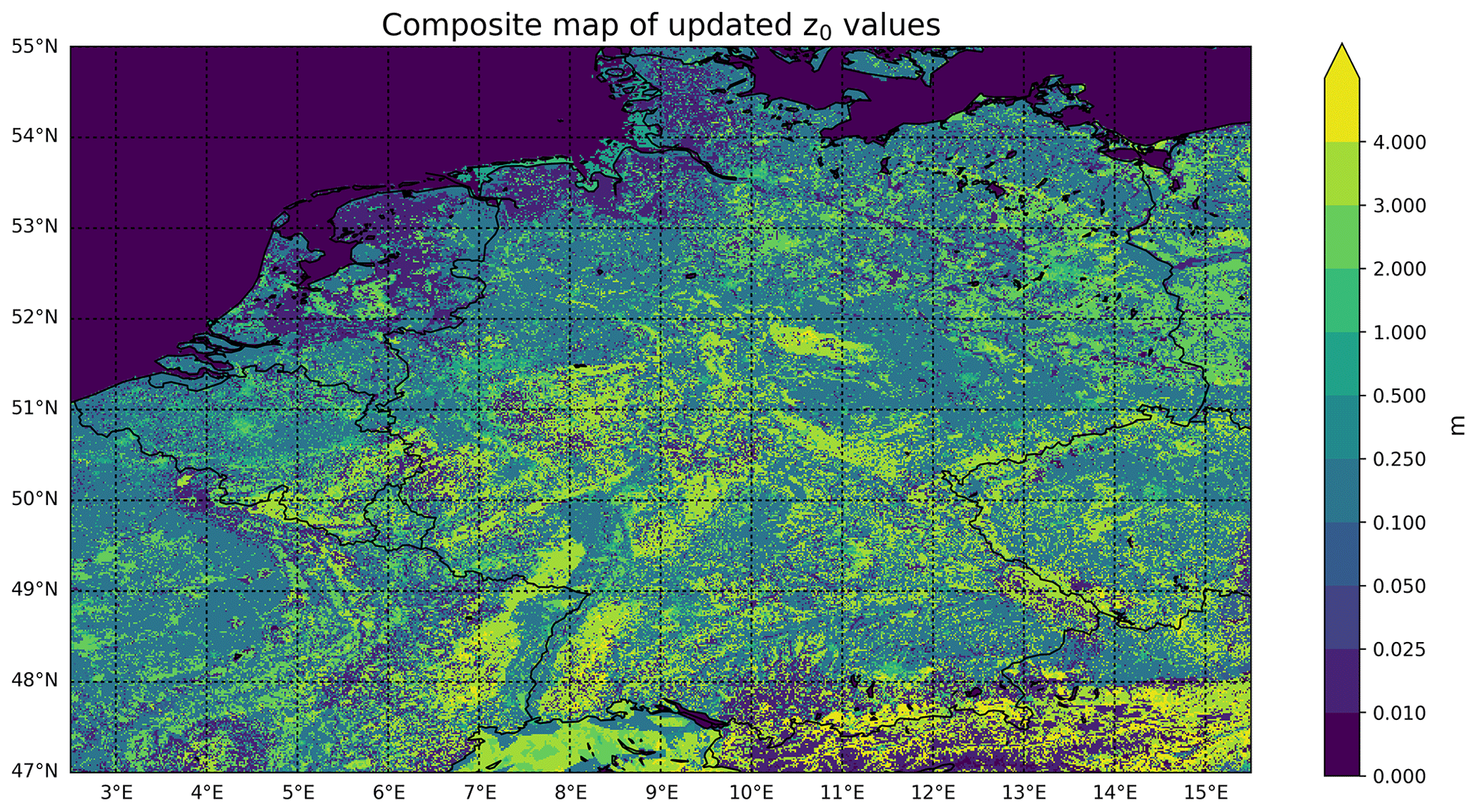
Figure 2Composite map of the new z0 values. The yearly mean is displayed for land use classes with time-variant z0 values.
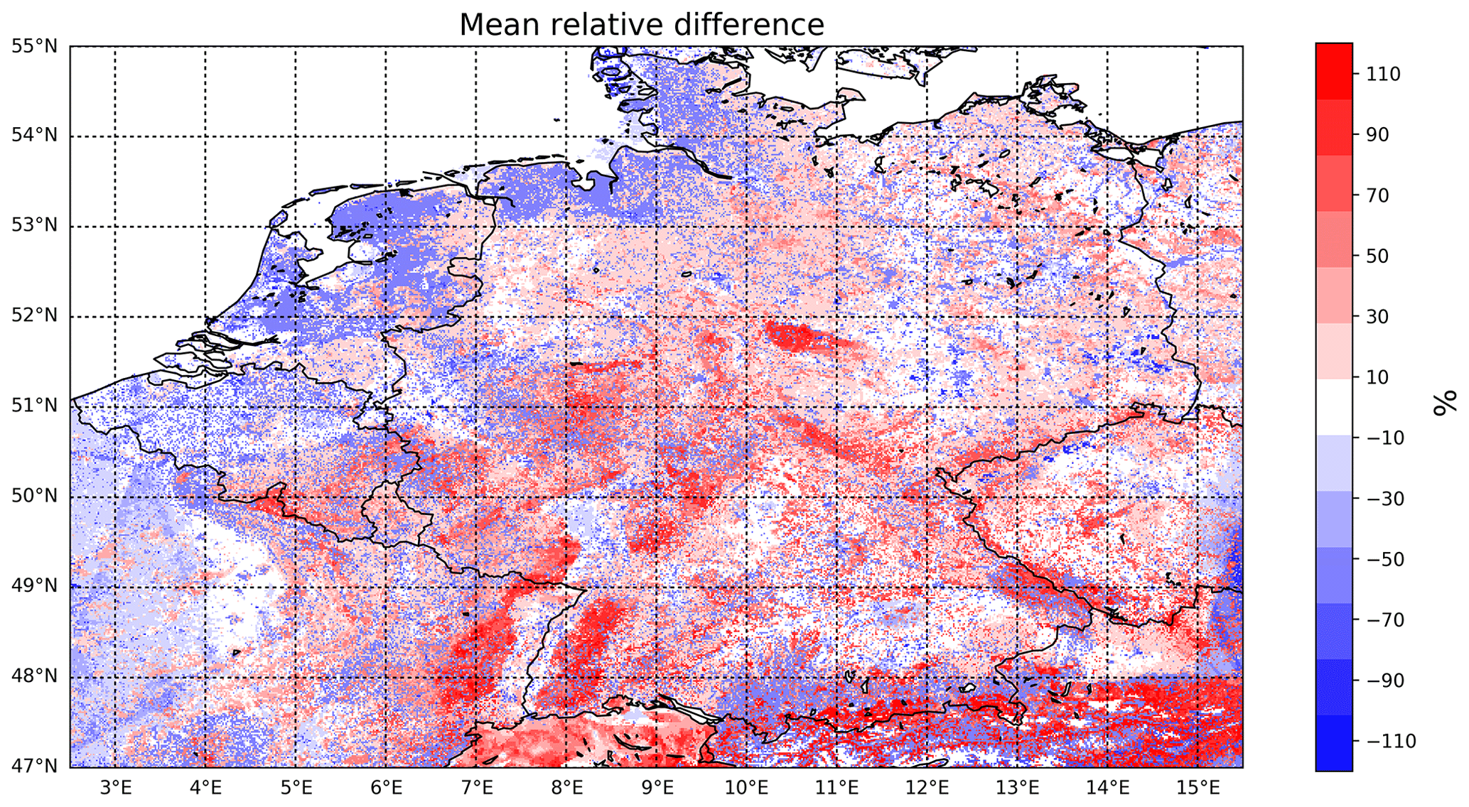
Figure 3Mean relative difference (%) of the updated z0 values with respect to the default z0 values.
Table 4An overview of the default and the adjusted roughness length of each DEPAC class used in LOTOS-EUROS for Germany, the Netherlands and Belgium. The datasets that are used to derive the updated z0 values are given in the last column. The mean z0 value of the DEPAC classes computed using the MODIS NDVI product is the yearly mean of all monthly z0 values.
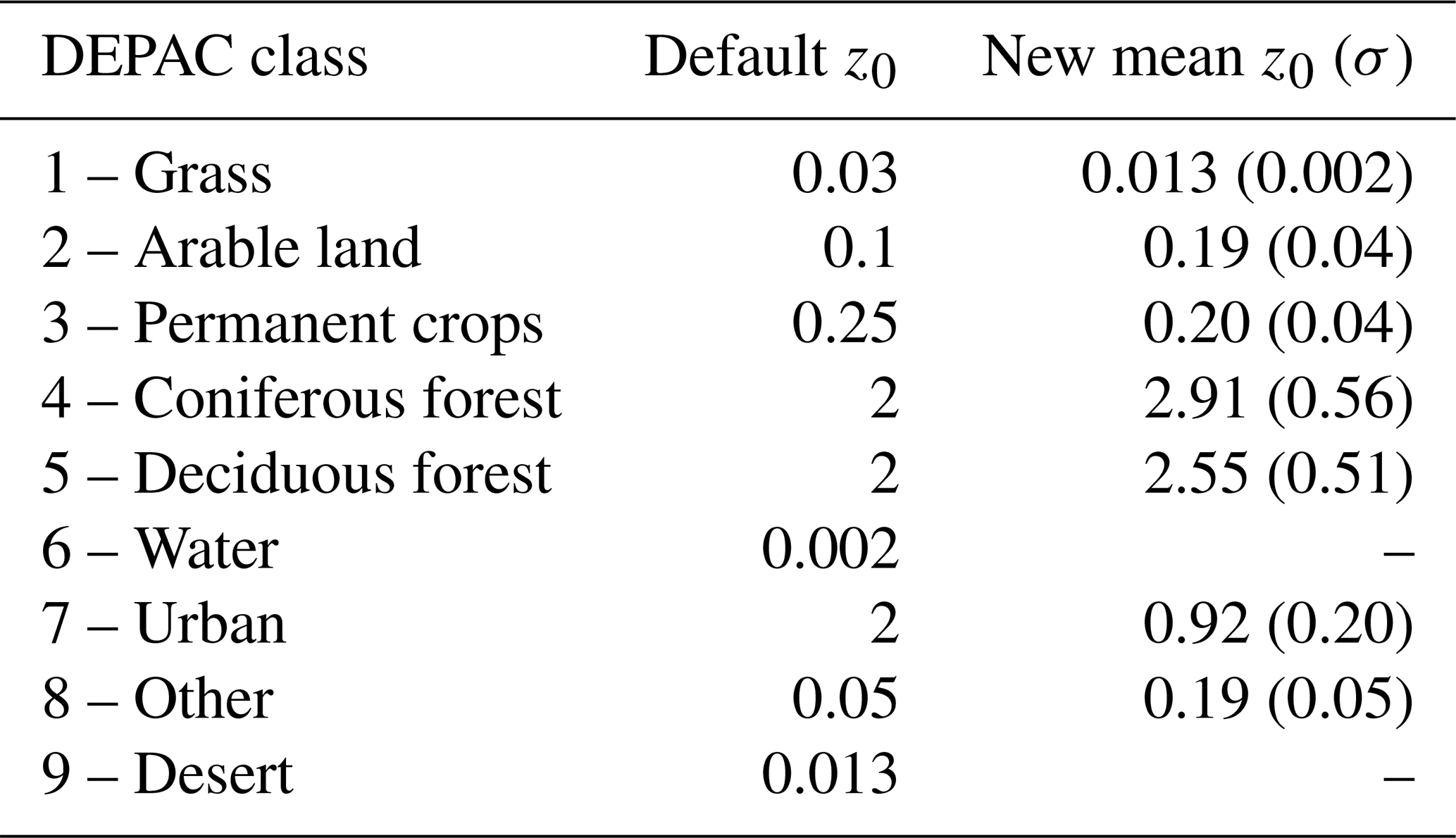
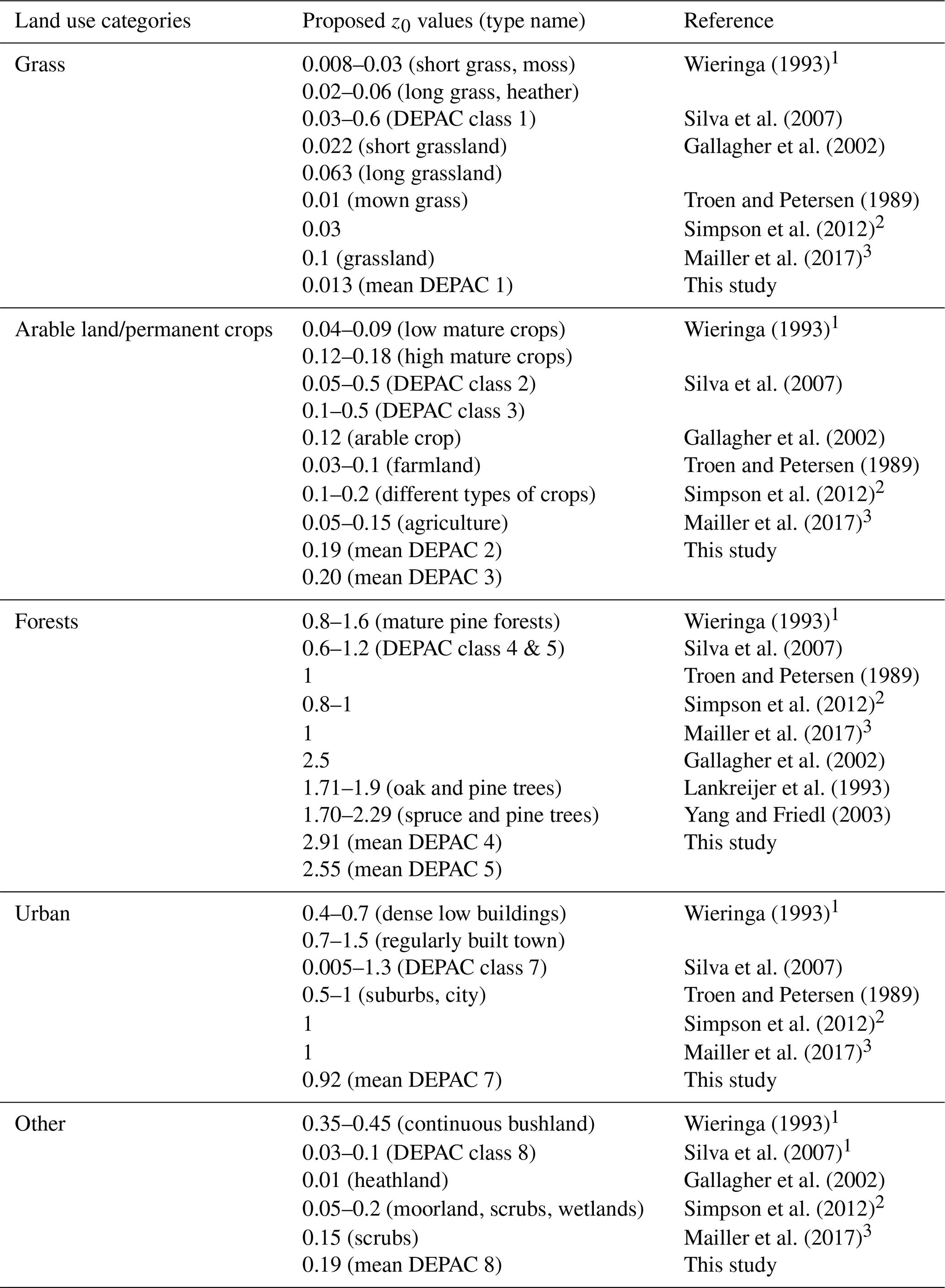
Table 5Roughness length values from different types of studies. The first column states the global land use category of the z0 values. The second column states the (range of) z0 values, as well as the specific type of land use they are derived for. The third column shows the reference. 1 Literature study. 2 Model input (EMEP Meteorological Synthesizing Centre – West; MSC-W). 3 Model input (CHIMERE).
3.1.2 NDVI-derived z0 values
Table 3 gives an overview of several studies that relate the z0 value to the NDVI. The functions are derived for different vegetation types under specific conditions. Equations (12)–(20) are derived for different types of agricultural land. These equations are all within a reasonable range from one another for NDVI values below ∼0.8. Therefore, we chose to use the average function of Eqs. (12)–(19) to compute z0 values for all CLC subcategories of the following DEPAC classes: “arable”, “other” and “permanent crops”. Figure 1 is a visualization of Eqs. (12)–(19) and the used mean function. Figure S1 in the Supplement shows a histogram of all NDVI values in our study area in 2014. We computed that 7.4 % of all NDVI values have a NDVI >0.8, 1.3 % have a NDVI >0.85 and only 0.04 % have a NDVI >0.9. Virtually all NDVI values thus fall within the range where the average function does not differ much from the individual functions. The z0 value of grasslands is in general lower than other vegetation types. The last equation, Eq. (20), is specifically derived for grassland and is therefore used for all CLC subcategories that fall under the DEPAC class “grass”.
3.1.3 z0 values for urban areas
The default z0 of urban areas in LOTOS-EUROS was set to 2 m. We have updated the z0 values for urban areas to avoid possible overestimation of z0 in sparsely populated urban areas. The updated z0 values for CLC2012 classes 1 and 2, “1: continuous urban fabric” and “2: discontinuous urban fabric” are time-invariant and coupled to the EEA population density map. The z0 values are set to 2 m in areas with a population density higher than 5000 inhabitants km−2 and to 1 m in areas with a population density lower than 5000 inhabitants km−2. The z0 values of the other urban subcategories, CLC2012 classes 3 to 9, are updated to the proposed values for CLC classes in Silva et al. (2007). Figure S2 shows the resulting updated z0 values for urban areas.
3.2 LAI and z0 in LOTOS-EUROS
After the computation of the z0 values, the maps for each CLC class were merged and converted into DEPAC classes using a pre-defined conversion table. As multiple CORINE land covers may translate to a single DEPAC class, the weighted average based on the respective percentage of each CORINE land cover class was computed for each pixel. We then used linear interpolation to obtain continuous z0 maps for each DEPAC class. Finally, the maps were regridded unto the CORINE/Smiatek grid and saved into one file per month.
The default parameterization of the LAI in LOTOS-EUROS is replaced by the MCD15A2H LAI product from MODIS. First, we applied a coordinate transformation to obtain the data in geographical coordinates. The data were then regridded unto the grid of the CORINE/Smiatek land use map using linear interpolation. The quality tags were evaluated to identify pixels with default fill values from the MCD15A2H product. These fill values were replaced by the default LAI values in LOTOS-EUROS, to avoid modelling discrepancies resulting from sudden jumps in LAI values. Finally, the values were sorted per DEPAC land use class and individual fields were created for each class as new input for LOTOS-EUROS.
4.1 Comparison of the default and updated z0 values
We used the CORINE/Smiatek land use map to combine all the updated z0 values into a single map. The resulting composite map has a horizontal resolution of 500 by 500 m and is shown in Fig. 2.
The mean relative difference (MRD) between the default and updated z0 values is presented in Fig. 3. The largest positive differences occur in forested areas, meaning that the default z0 values are lower than the updated z0 values. The largest negative deviations occur in urban areas and areas with “grass”. The updated z0 values are generally lower in the Netherlands and Belgium, and mostly higher in Germany. Table 4 gives an overview of the default z0 values in LOTOS-EUROS and the mean and standard deviation of the new z0 values for each of the DEPAC land use classes. The updated z0 values for “arable land”, “coniferous forest”, “deciduous forest” and “other” are on average higher than the default z0 values in LOTOS-EUROS. The updated z0 values for “grass”, “permanent crops” and “urban” are on average lower than the default z0 values in LOTOS-EUROS.
Table 6Comparison of the computed z0 values from FLUXNET observations and the corresponding satellite-derived z0 values. The table shows the mean and standard deviation of all z0 values in 1 year. For forest, only the maximum z0 value is given.
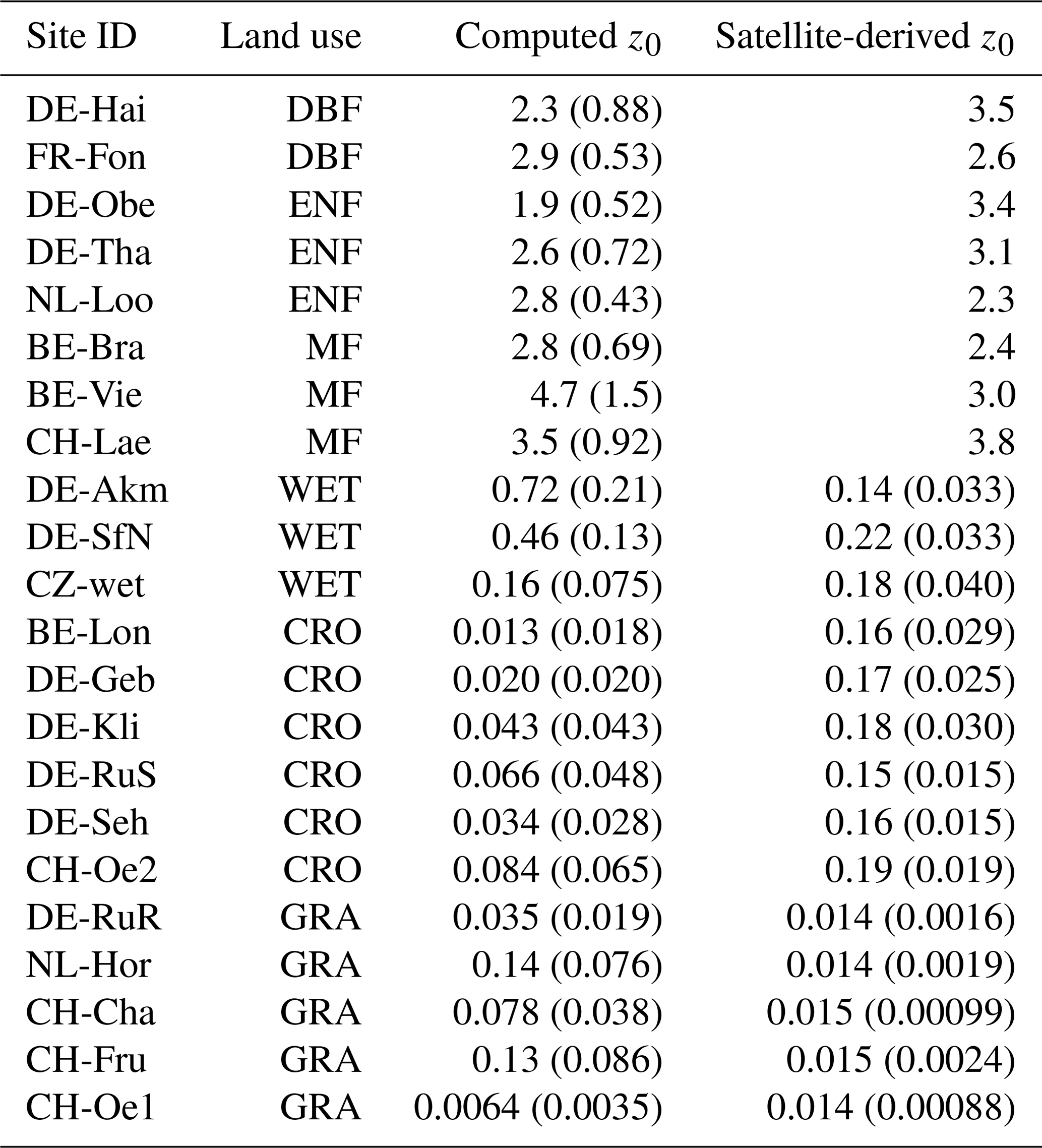
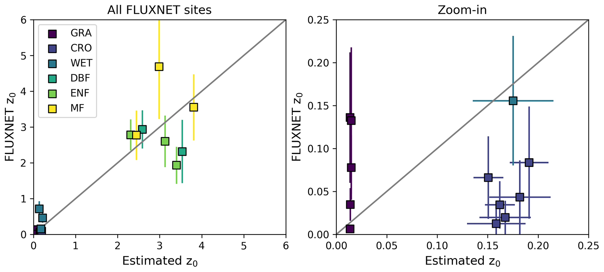
Figure 4Comparison of the updated z0 values (x axis) to the z0 values derived from EC measurements (y axis). The error bars indicate the standard deviation.
4.2 Comparison to z0 values from other studies
We compared the updated z0 values to z0 values from several studies (Wieringa, 1993; Silva et al., 2007; Troen and Petersen, 1989; Lankreijer et al., 1993; Yang and Friedl, 2003) and z0 values used in other CTMs (Simpson et al., 2012; Mailler et al., 2017). Table 5 gives an overview of these z0 values. There is in general good agreement with these z0 values, and the updated z0 values mostly fall within the stated ranges. The updated z0 values for coniferous and deciduous forest are on the high side compared to these studies. A histogram of the forest canopy heights derived from GLAS within our study area is given in Fig. S1 in the Supplement. These differences can in part be explained by the occurrence of relatively tall forest canopy (∼30 m) in the dataset, especially in forests in southern Germany, whereas most of these studies either assumed or studied shorter trees. Another possible explanation lies in the fact that we used a relatively large conversion factor of 0.136 (Eq. 12), whereas a factor of 0.10 is also used quite often.
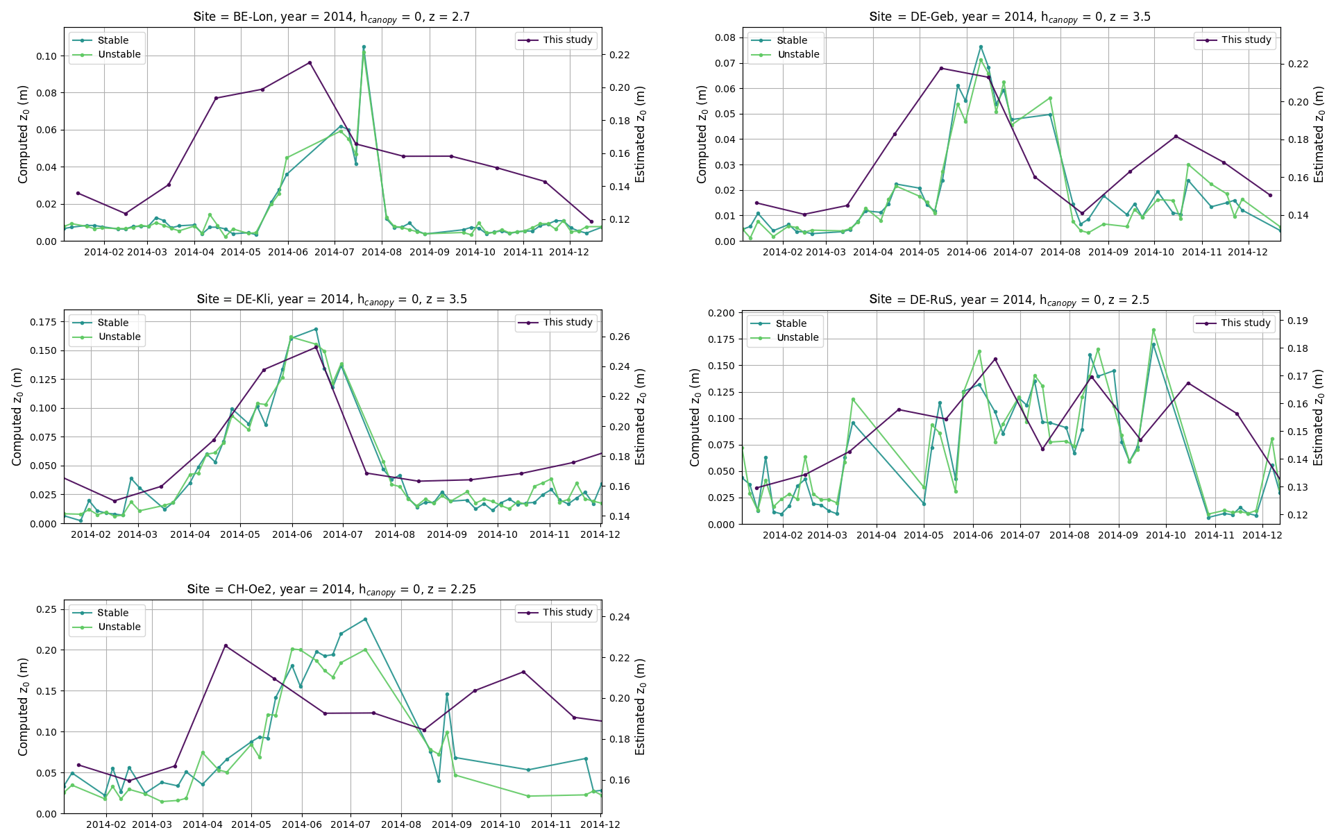
Figure 5Seasonal variation of the computed z0 values at the FLUXNET cropland sites in 2014 (left axis) and the corresponding z0 values estimated from NDVI values (right axis). The green lines indicate the estimated z0 values derived from FLUXNET measurements and the purple lines indicate the z0 values derived from NDVI values. The assumptions used to compute the z0 values are shown in the titles of the figures.
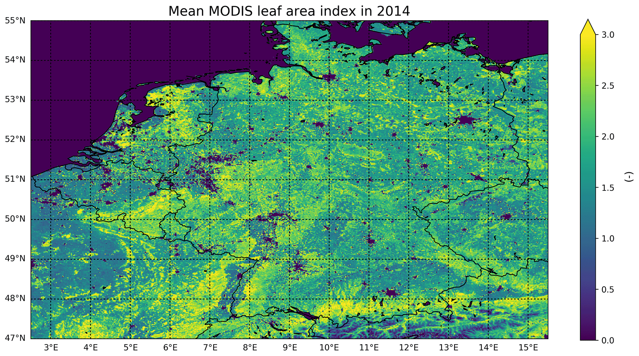
Figure 6The yearly mean MODIS leaf area index in 2014.
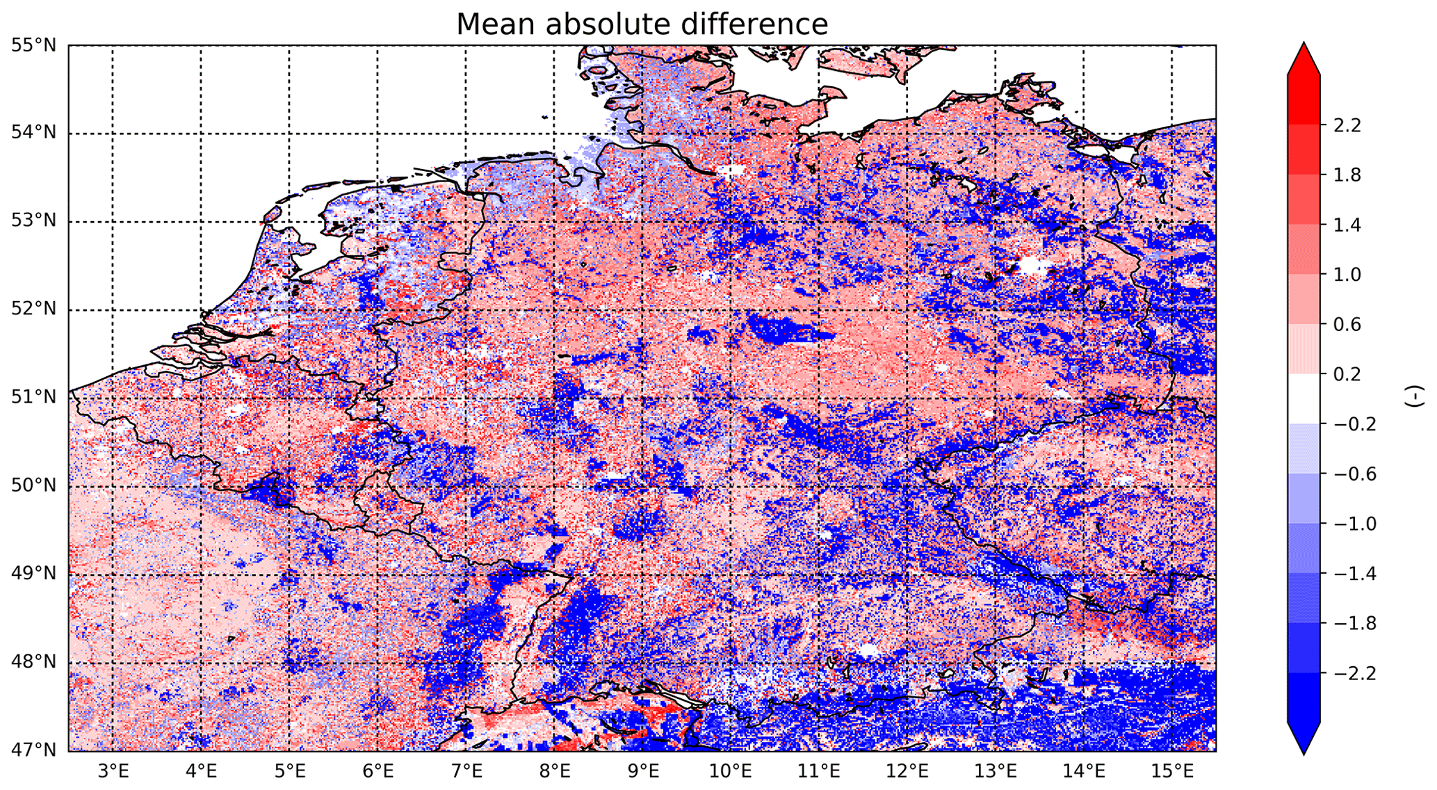
Figure 7The absolute differences (LAIMODIS – LAIdefault) between the MODIS leaf area index and the default leaf area index in LOTOS-EUROS.
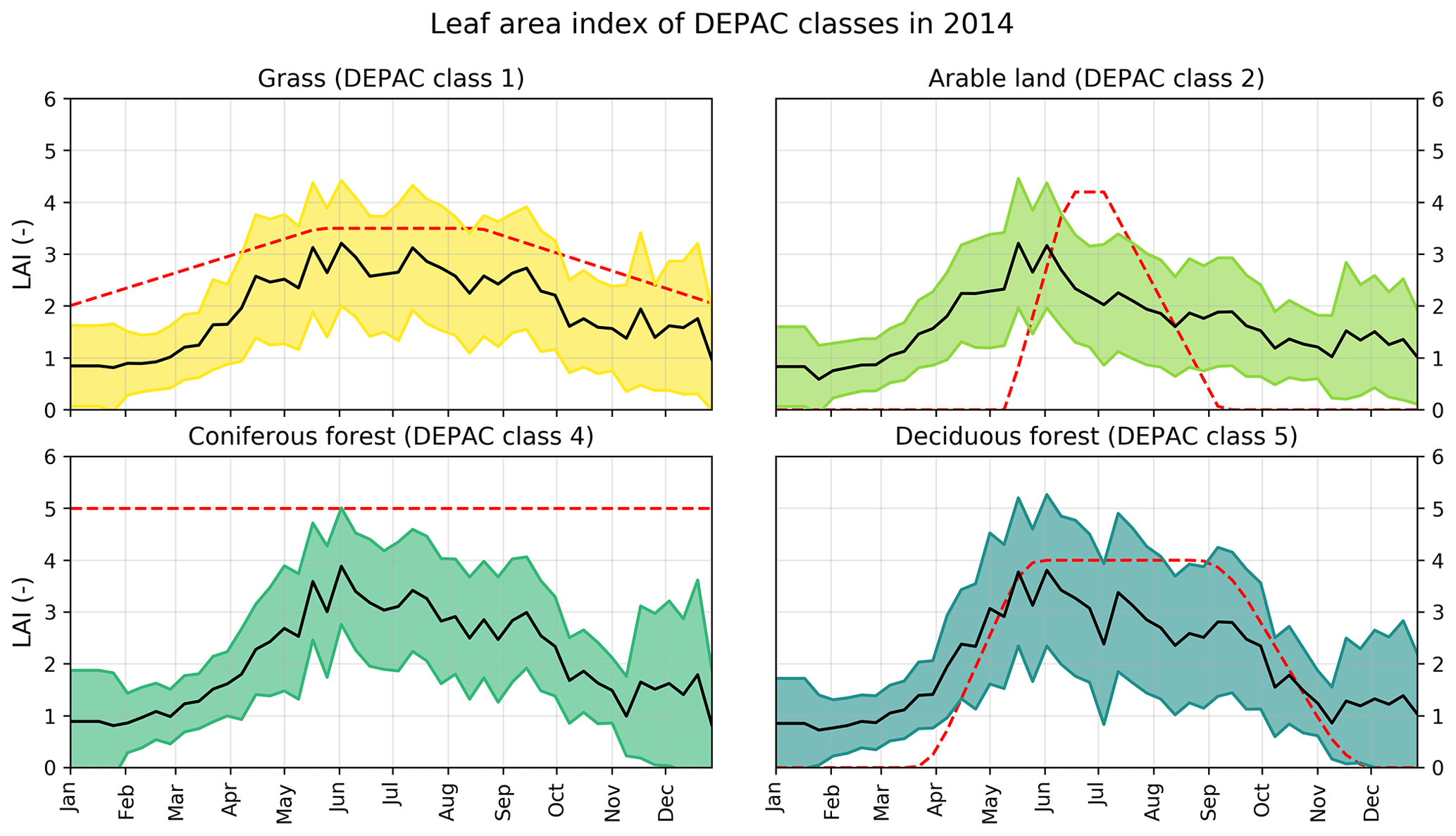
Figure 8Seasonal variation of the default and MODIS LAI values per DEPAC class. The black line represents the mean MODIS LAI of all pixels within the modelled grid for that particular DEPAC class; the ranges represent the mean plus and minus the standard deviation of the MODIS LAI. The red line depicts the default LAI values in LOTOS-EUROS.
4.3 Comparison to z0 values derived from EC measurement sites
We computed the z0 values of the EC sites, and we refer to Sect. S1 in the Supplement for a description of the methodology that is used to derive these values. We compared the z0 values based on their land use stated by FLUXNET to avoid issues arising from discrepancies in land use classifications. The forest sites (DBF, ENF and MF) are compared to z0 values derived from GLAS. The cropland and wetland sites (CRO and WET) are compared to the NDVI-dependent z0 values derived using the mean function shown in Fig. 1. The grassland sites (GRA) are compared to the NDVI-dependent z0 values for grassland specifically. The results per site are given in Table 6. Figure 4 shows the comparison of the z0 values from EC measurements and the updated z0 values for different land use classes. The z0 values for forests match quite well. Differences between the two can in part be explained by the influence of topography, which is not accounted for in the z0 values that are derived using forest canopy height only. The z0 values for short vegetation seem to be overestimated for crops and underestimated for grassland and wetland sites. The underestimation of some grassland and wetland sites can be explained by the large inter-site differences in vegetation cover. Some of the FLUXNET sites classified as grasslands are, for instance, mostly covered with short grass only (for instance, Oensingen), while other sites are covered with relatively tall herbaceous vegetation, such as reeds (for instance, Horstermeer). Compared to the default z0 values in LOTOS-EUROS, the root mean square difference (RMSD) improved from 0.76 (default z0) to 0.60 (updated z0). For forest, the RMSD improved from 1.23 (default z0) to 0.96 (updated z0). For short vegetation, the RMSD also decreased, from 0.22 (default z0) to 0.19 (updated z0). Figure 5 shows the comparison of the seasonal variation in computed and satellite-derived z0 values for the FLUXNET sites classified as crops in 2014. We can once more observe a clear offset between the two. The FLUXNET z0 values go to near-zero values in wintertime, whereas the satellite-derived z0 values never drop below 0.12 m. This seems to be due to the distribution of the NDVI values (Fig. S1), which shows that the NDVI >0.4 most of the time. The seasonal patterns, on the other hand, seem to match well in general, even though the satellite-derived z0 values rise somewhat earlier in the year.
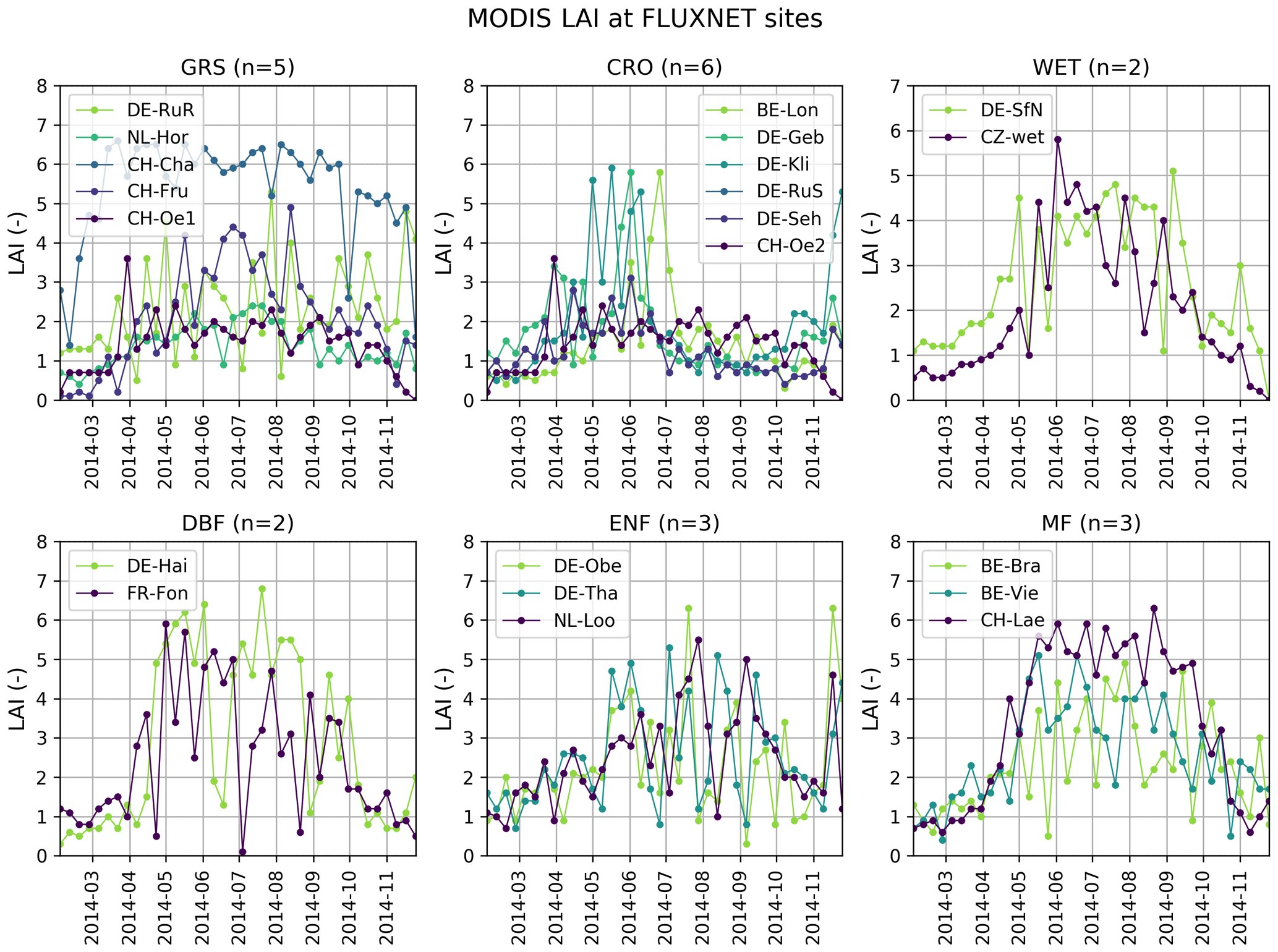
Figure 9Seasonal variation of the MODIS LAI at individual FLUXNET sites with different land use classifications.
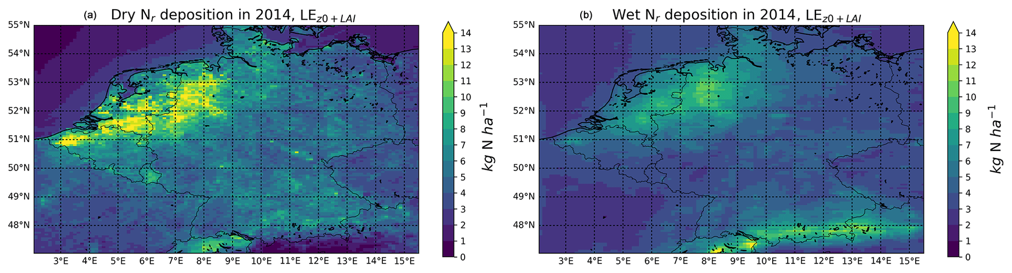
Figure 10The modelled amount of dry (a) and wet (b) deposition in kg N ha−1 in 2014.
4.4 Comparison of the default and MODIS LAI
The yearly mean MODIS LAI values are shown in Fig. 6. The mean differences between the MODIS and the default LAI values are presented in Fig. 7. The largest positive differences occur in areas with “arable land”, where the mean default LAI values are lower than the MODIS LAI values. The largest negative deviations occur in areas with forest, especially for “coniferous forest”. The seasonal variations of the MODIS and the default LAI values are shown in Fig. 8. The default LAI of “grass” and “deciduous forest” seems to fit the yearly variation of the MODIS LAI quite well. We matched the MODIS LAI with the locations of the FLUXNET sites to take a closer look at the pattern for different land use classes. Figures 9 and S3 show the seasonal variation of the MODIS LAI at FLUXNET sites with different land use classifications. The LAI of the grassland sites seems to vary the most, which corresponds to the large inter-site differences in vegetation cover as explained in Sect. 4.3. For the cropland sites, we can recognize the growing season and the apparent harvest, where the LAI values drop again. Of all the different land use classes, deciduous broadleaf forest sites reach the highest LAI values in the growing season. There is less variation in the LAI for evergreen needleleaf forest sites. However, the wintertime LAI values seem to be unrealistically low.
4.5 Implications for modelled Nr deposition fields
In the following section, the impact of the updated LAI and z0 values on modelled Nr deposition fields in LOTOS-EUROS is discussed. A total of four different LOTOS-EUROS runs are compared to examine the individual effect of the updated LAI and z0 values on the modelled Nr distributions and deposition fields. The first run, named “LEdefault”, is the standard run using default LAI and z0 values. The second run, named “LELAI”, uses updated LAI values and the default z0 values. The third run, named “LEz0”, uses updated z0 values and the default LAI values. The fourth run, named “LEz0+LAI”, uses both updated LAI and z0 values. From now on, we will refer to the outputs of these different runs using the abovementioned abbreviations.
4.5.1 Effect on total Nr deposition
Figure S4 shows the division of the total terrestrial Nr deposition over Germany, the Netherlands and Belgium into different Nr compounds for each of the model runs. A relatively larger portion of the total Nr deposition is attributed to oxidized forms of Nr in Germany. The reduced forms of Nr predominate in the Netherlands and Belgium. The largest change in total Nr deposition occurs in Belgium (+6.19 %) due to the inclusion of the MODIS LAI. This corresponds to the relative increase in LAI values here. The inclusion of the updated z0 values led to a minor decrease in total Nr deposition in the Netherlands (−1.45 %) and Belgium (−1.13 %), and a minor increase in Germany (+0.44 %).
4.5.2 Effect on wet and dry Nr deposition
We examined the direct effect of the updated LAI and z0 values on the modelled dry Nr deposition, as well as the related indirect effect in modelled wet Nr deposition. Figure 10 shows the dry and wet Nr deposition in kg N ha−1 in 2014, modelled with the updated LAI and z0 values as input in LOTOS-EUROS. Figure 11 shows the relative changes in the total amount of dry and wet Nr deposition of the different runs with respect to the default run. The combined effect shows an increase of the amount of dry Nr deposition over most parts of Belgium and Germany. The amount of wet Nr deposition decreases over most parts of Germany and eastern Belgium but remains unchanged in north-western parts of Germany. We observe a decrease in total Nr deposition in the Netherlands. In general, we observe changes ranging from approximately −20 % to +30 % in the total amount of dry Nr deposition. The changes in wet Nr deposition are smaller in magnitude and range from approximately −3 % to +3 %.
4.5.3 Effect on reduced and oxidized Nr deposition
We split up the total Nr deposition into NHx (NH3 and ) and NOy (NO and NO2 and and HNO3) deposition to look at the effect of the updated LAI and z0 input maps on the deposition of reduced and oxidized forms of Nr, respectively. Figure 12 shows the modelled NHx and NOy deposition in kg N ha−1 in 2014, including the updated LAI and z0 input values. Figure 13 shows the relative changes (%) in the total NHx and NOy of the different runs with respect to the default run of LOTOS-EUROS. The updated z0 values have a larger impact on the NHx deposition than on the NOy deposition. The implementation of the updated z0 values has led to a decrease in NHx deposition over most of the Netherlands and western Belgium, driven by the large fraction of grassland here. The updated LAI values led to relatively more NHx deposition in Belgium. The updated LAI values led to an increase of NOy deposition in almost all areas within the modelled region, except for some urban areas. Moreover, the impact seems to be limited in large forests located in background areas.

Figure 11The relative change in total dry (a, b, c) and wet (d, e, f) Nr deposition in 2014 for the different model runs relative to the default LOTOS-EUROS run. The first row indicates the changes related to the implementation of the updated z0 values. The second row indicates the changes related to the implementation of the MODIS LAI values. The third row shows the combined effect of both these updates. (Please note the different scales).
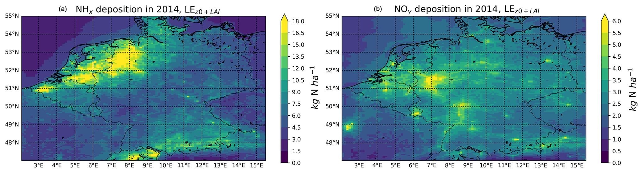
Figure 12NHx deposition (a) and NOy deposition (b) in kg N ha−1 in 2014.
Table 7Relative change (%) in total Nr deposition with respect to the default run over Germany, the Netherlands and Belgium in 2014 per land use class.

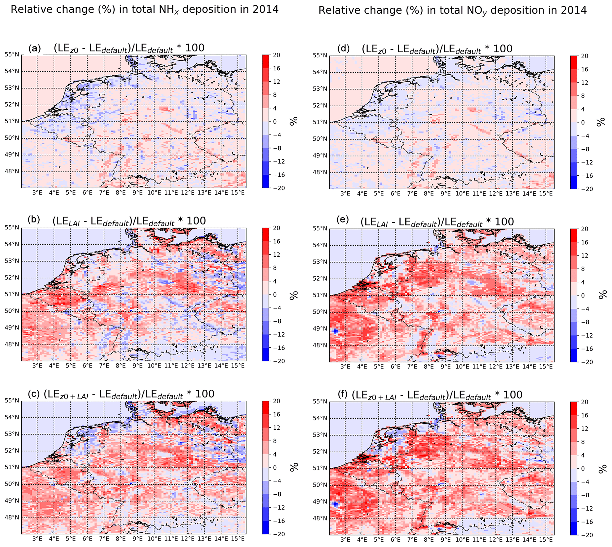
Figure 13The relative change in total NHx (a, d) and NOy (c, f) deposition in 2014 for the different model runs relative to the default LOTOS-EUROS run. The first row indicates the changes related to the implementation of the updated z0 values. The second row indicates the changes related to the implementation of the MODIS LAI values. The third row shows the combined effect of both these updates.
4.5.4 Effect on land-use-specific fluxes
Table 7 gives an overview of changes in the distribution of the land-use-specific fluxes in the whole study area (Germany, the Netherlands and Belgium combined) for the different runs. The most distinct changes in Nr deposition are due to the updated LAI values (“LELAI”), where we observe an increase in total Nr deposition on urban areas (+16.62 %) and arable land (+9.53 %), and a decrease on coniferous forests (−9.36 %). This coincides with the categories where we observe the largest changes in LAI values. The default LAI values in urban areas were first set to zero for all urban DEPAC categories. The MODIS LAI values, however, are only zero in densely populated areas and areas with industry. The main effects of the updated z0 values (“LEz0”) can be observed for grass (−3.95 %), permanent crops (+3.27) and arable land (−3.17 %). In the combined run, “LEz0+LAI”, we observe an amplified effect in total Nr deposition over grass (−8.05 %) and arable land (+12.88 %). The impact of the individual parameters on the remaining land use categories is attenuated in this run.
4.6 Implications for Nr distributions
The changes in Nr deposition amounts induce an effect in the modelled distribution of nitrogen components. Here, we look at the effect of the updated LAI and z0 values on NH3 and NO2 surface concentrations. Figure 14 shows the updated modelled NH3 and NO2 surface concentrations in 2014. The dots on top of the figures represent the stations that are used for validation and their observed mean NH3 and NO2 surface concentrations. Figure 15 shows the relative change in yearly mean NH3 and NO2 surface concentrations in 2014 of the different runs with respect to the default run of LOTOS-EUROS.
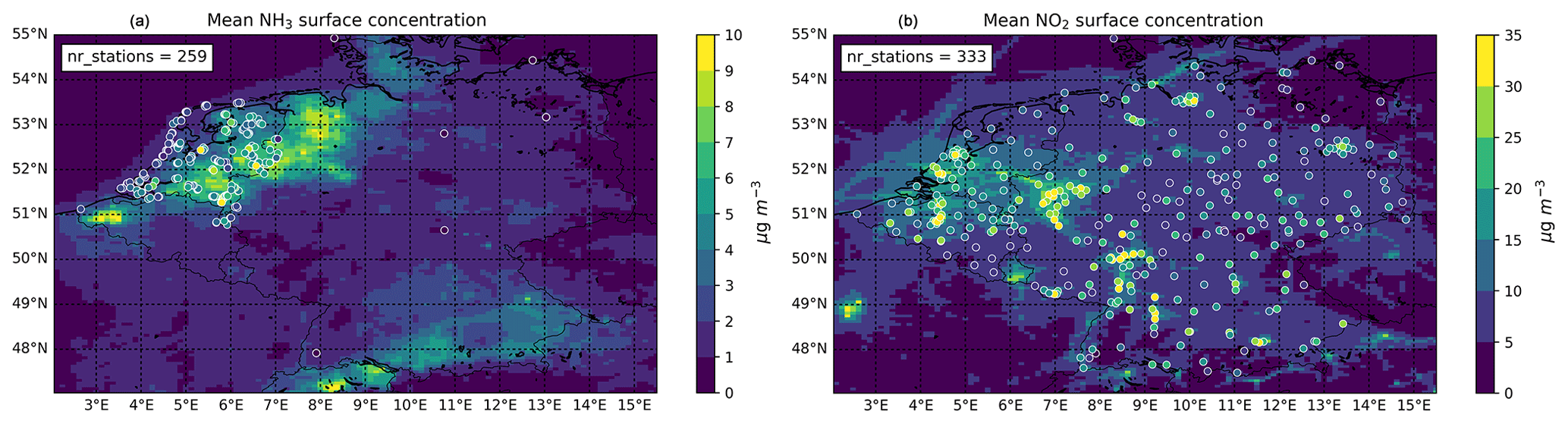
Figure 14The yearly mean NH3 (a) and NO2 (b) surface concentrations in µg m−3 in 2014 and the corresponding mean surface concentrations measured at the in situ stations.
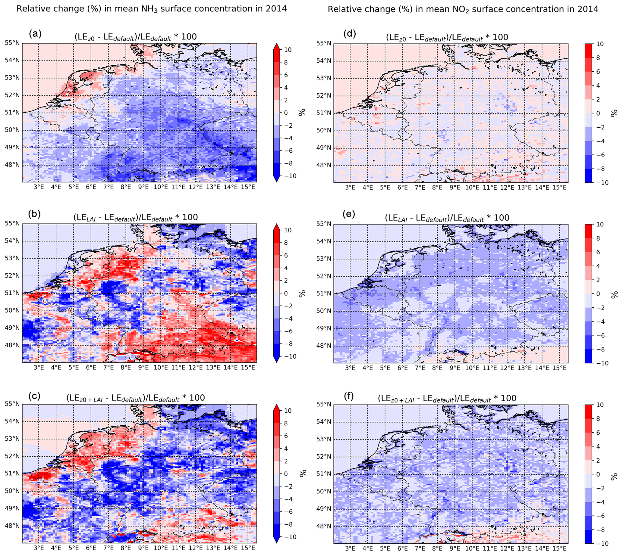
Figure 15The relative change (%) in mean NH3 (a, b, c) and NO2 (d, e, f) surface concentration in 2014 for the different model runs relative to the default LOTOS-EUROS run. The first row indicates the changes related to the implementation of the updated z0 values. The second row indicates the changes related to the implementation of the MODIS LAI values. The third row shows the combined effect of both these updates.
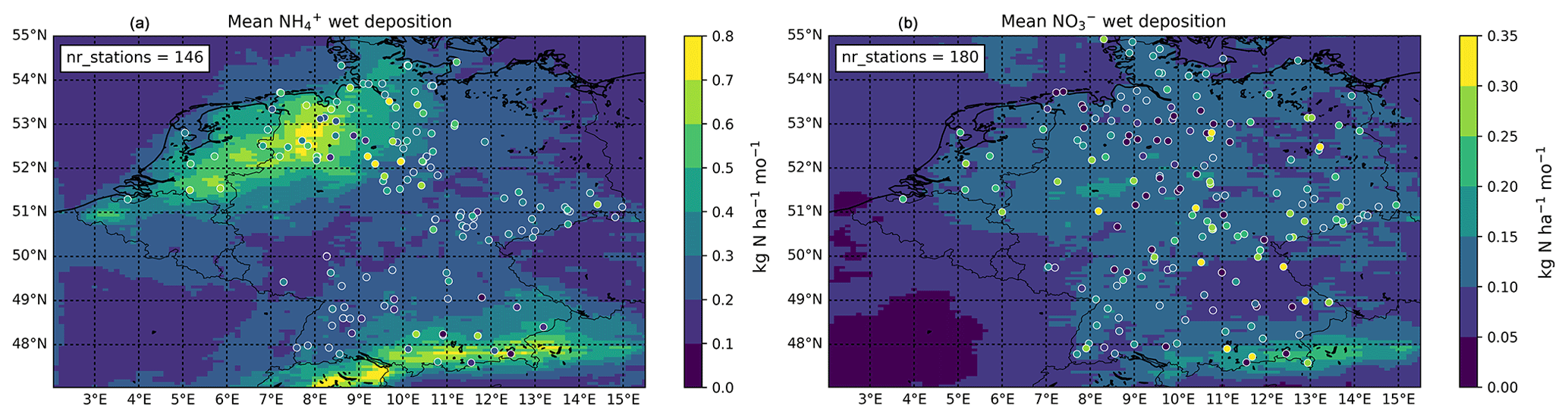
Figure 16The mean (a) and (b) wet deposition in kg N ha−1 month−1 in 2014. The mean observed wet deposition observed at the stations is plotted on top.
The first column represents the changes in NH3 and NO2 surface concentrations due to the updated z0 values. The NH3 surface concentration in the Netherlands has increased by up to ∼8 %. The NH3 surface concentration in almost all of Germany has decreased by up to ∼10 %. The changes in the NO2 surface concentration are less distinct and changed approximately minus to plus 4 % in most areas. The middle column represents the changes in NH3 and NO2 surface concentrations due to the inclusion of the MODIS LAI only. The NH3 surface concentration has increased with up to ∼10 % in the Netherlands, western Belgium and north-western and southern Germany. The NH3 surface concentration has decreased in eastern Belgium and central Germany. The NO2 surface concentrations have decreased with up to ∼6 % in almost all of the modelled area.
4.7 Comparison to in situ measurements
To analyse the effect of the updated LAI and z0 values, we compared our model output to the available in situ observations. Due to the lack of available dry deposition measurements, we decided to use and wet deposition and NH3 and NO2 surface concentrations measurements instead. The distribution of the wet deposition stations is shown in Fig. 16, as well as the modelled mean (left) and (right) wet deposition in 2014. The locations of the stations that measure the NH3 and NO2 surface concentrations are shown in Fig. 14.
The relationships between the modelled and observed fields are evaluated using the Pearson correlation coefficient (r), the RMSD and the coefficients (slope, intercept) of simple linear regression. Table S1 shows these measures for the comparison with monthly mean wet deposition, wet deposition and the monthly mean NH3 and NO2 surface concentrations in 2014. Table S1 shows the same statistics but computed per DEPAC land use class. Overall, we do not observe large changes in the shown measures due to the inclusion of the updated LAI and z0 values on a yearly basis. The model underestimates wet deposition, and to a lesser extent, too. The modelled NH3 surface concentrations are in general higher than observed concentrations. The opposite is true for NO2; here, the modelled surface concentrations are lower than the observed concentrations. The computed measures did not change drastically due to the inclusion of the updated z0 and LAI values.
Figure S5 shows the monthly mean wet deposition, wet deposition, NH3 surface concentration and NO2 surface concentrations for the different model runs and the mean of the corresponding in situ observations. The relative changes with respect to the default model run are shown in the bottom figures. For , the model captures the observed pattern quite well, although the mean spring peak has slightly shifted. The model captures the monthly variation of well in general, too. There appears to be an underestimation during the winter, especially in December. The observed NH3 surface concentrations are lower than the modelled concentrations at the beginning of spring and higher during summer. The measured NO2 surface concentrations are continuously higher than the modelled values. A potential reason for this might be the spread of the NO2 stations. Unlike NH3, NO2 is not only measured in nature areas but all types of locations. Even the selected background stations may therefore be located relatively closer to emission sources, leading to higher observed NO2 surface concentrations. The changes due to the inclusion of either the MODIS LAI or the updated z0 values in our model are limited.
Both Tables S1 and S2, and Fig. 16 illustrate that the comparability of the modelled wet deposition and surface concentration fields to the available in situ measurements did not change significantly. The impact of the updated LAI and z0 values on these fields is largely an indirect effect of the more distinct changes in the dry deposition and thus too small to lead to any drastic changes. We conclude that we are unable to demonstrate any major improvements with the use of the currently available in situ measurements.
This paper aimed to improve the surface characterization of LOTOS-EUROS through the inclusion of satellite-derived LAI and roughness length (z0) values. We used empirical functions to derive z0 values for different land use classes. The updated z0 values are compared to literature values, showing a good agreement in general. We also compared our z0 values to z0 values computed from FLUXNET sites. The z0 values for forests seemed to match well, but the z0 values for short vegetation seem to be overestimated for crops and underestimated for grassland and wetland sites. The differences for short vegetation types can be partially explained by the large inter-site variability in vegetation types within each classified land use (e.g. reeds versus short grass). The equation for short vegetation used here seems to work best for short grasslands. For our current study area, this does not pose a problem, since most grasslands in Germany, Belgium and the Netherlands are managed and grazed upon. We found an improved RMSD value of 0.60, compared to RMSD of 0.76 with default z0 values. Even though there is an offset between the satellite-derived and computed FLUXNET z0 values for crops, the seasonal pattern seemed to match well. The offset can be explained by the absence of low NDVI (<0.4) values.
The z0 is closely related to the geometric features and distributions of the roughness elements in a certain area. In reality, it is not only dependent on vegetation properties but, for instance, also the topography of the area. The updated z0 values are linked to specific land use pixels and are therefore assumed reasonable estimates for moderately homogeneous areas with this specific land use type. There are various approaches to combine these z0 values into an “effective” roughness for larger, mixed areas (e.g. Claussen, 1990; Mason, 1988). The LOTOS-EUROS model uses logarithmic averaging to compute an effective roughness for an entire model pixel. This averaging step seems to be one of the reasons why the effect of our updated z0 values on the deposition fields is limited. To illustrate this, the relative change in total dry NH3 deposition due to the updated z0 values were computed and shown in Fig. 17. We used increasing threshold percentages to sort the NH3 deposition on a model pixel level per land use type and fraction. Figure 17 shows that the differences in total NH3 deposition between the two runs increase with increasing land use fraction. The model pixels that mostly consist of one type of land use seem to show the largest change in NH3 deposition. The change thus appears to be less distinct in pixels that have a higher degree of mixing. Most of the model pixels largely contain mixtures of different land uses on the current model resolution. As a result, averaging of z0 on a model pixel level is thus likely to cause a levelling effect on the current model resolution. The impact of the updated z0 values is therefore expected to be larger at a higher model resolution. The use of another approach for computing the “effective” roughness could potentially lead to stronger changes in the modelled deposition fields.
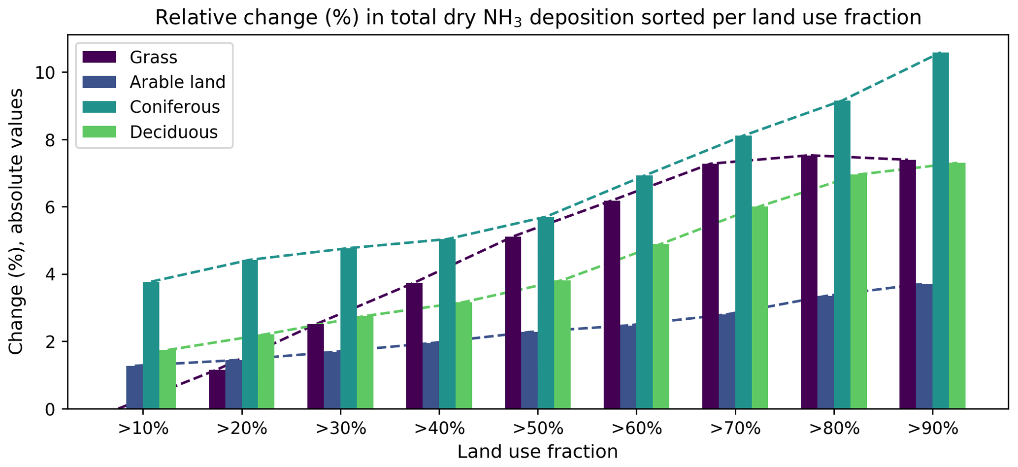
Figure 17The relative difference (%) in total dry NH3 deposition in 2014 between the default run (LEdefault) and the run with the updated z0 values (LEz0), sorted by increasing land use fraction.

Figure 18Critical load exceedances on forests in kg N ha−1 in 2014. The upper figures show the critical on deciduous (a) and coniferous (b) forest, as modelled with the updated z0 and LAI values. The lower figures show the absolute differences in critical load exceedance on deciduous (c) and coniferous (d) between the new and the default LOTOS-EUROS run.
Moreover, we should also consider the limitations of the datasets used in this study. The forest canopy height map used in this study has been validated against 66 FLUXNET sites (Simard et al., 2011). The results showed that root mean square error (RMSE) was 4.4 m and R2 was 0.7 after removal of seven outliers. For the FLUXNET forest sites used in this study, we compared the forest canopy heights from GLAS to the maximum forest canopy height at the FLUXNET sites taken from (Flechard et al., 2020). For all but one site (DE-Hai), the forest canopy heights from GLAS were lower than this value (Table S3). This method could potentially be improved by using another product with either a higher precision or resolution. For modelling studies on a national level, one could or instance consider the use of airborne lidar point clouds to retrieve forest canopy heights. This procedure, although it is computationally expensive, would allow us to create high-resolution z0 maps.
The MODIS LAI at the FLUXNET sites showed realistic seasonal variations for most land use classifications, except for relatively low wintertime values for evergreen needleleaf forests. The previous versions of the MODIS LAI have been validated in many studies (e.g. Fang et al., 2012; Wang et al., 2004; Kobayashi et al., 2010), showing an overall good agreement with ground-observed LAI values and other LAI products. The seasonality in LAI is properly captured for most biomes, but unrealistic temporal variability is observed for forest due to infrequent observations. Also, the previous versions overestimate LAI for forests (Fang et al., 2012; Kobayashi et al., 2010; Wang et al., 2004). The MODIS LAI products have been gradually improving with each update; however, these issues still exist in the newer versions of the product. For the most recent version of the MODIS LAI, version 6, Yan et al. (2016) found an overall RMSE of 0.66 and a R2 of 0.77 in comparison with LAI ground observation. More recently, using a different approach, Xu et al. (2018) found a slightly higher RMSE of 0.93 and a R2 of 0.77. Some studies (e.g. Tian et al., 2004) have reported an underestimation of the MODIS LAI in presence of snow cover, particularly affecting evergreen forests. With only limited amounts of snowfall, the regions in our study did not suffer from this problem. However, this issue should be carefully considered when using the MODIS LAI for regions with frequent snow cover, like Scandinavia. LOTOS-EUROS uses meteorological data to determine what regions are covered with snow and for these regions the standard parameterization for the canopy resistance is not used. LOTOS-EUROS uses a pre-defined value for the canopy resistance instead. As such, these low MODIS LAI values do not affect the modelled deposition in LOTOS-EUROS during snow cover.
Though the issues with the MODIS LAI should be considered with care, the spatial and temporal distributions of these LAI values are more realistic than those of the default LAI values used in LOTOS-EUROS. The same holds for the updated, time-variant z0 values. The representation of the growing season is now more realistic due to their dependence on NDVI and LAI values. Moreover, the z0 values for forests now also have a clear spatial variation, such as a latitudinal gradient with increasing z0 values towards the south of Germany. These type of patterns can simply not be captured by fixed values.
We evaluated the effect of updated z0 and LAI values on modelled Nr distribution and deposition fields. The distribution of the relative changes in deposition of the reduced and oxidized forms of reactive nitrogen showed a similar pattern. Here, the updated z0 values led to a variation of %, and the updated LAI values led to variations of % in both fields. The dry deposition fields were most sensitive to changes in z0 and LAI, as these varied from approximately −20 % to +20 % with the updated z0 map, and from −20 % even up to +30 % with the MODIS LAI values. As a result, we observed a shift from wet to dry deposition, except for the Netherlands, where we observe an opposite shift from dry to wet deposition. Moreover, we observed a redistribution of Nr deposition over different land use classes on a subgrid level. To illustrate the potential consequences on a local scale, we computed the critical load exceedances for deciduous and coniferous forest (Fig. 18) using critical loads of 10 kg following Bobbink et al. (2010b). Compared to the default run, the changes may be sizable locally, ranging from approximately −3 up to +2 kg for deciduous forest and even over −3 kg for coniferous forest.
The uncertainties of the LAI and z0 input data are but one aspect of the model uncertainty of CTMs. The model uncertainty has several other origins, like the physical parameterizations (e.g. deposition velocities) and the numerical approximations (e.g. grid size). Two of the most important uncertainties related to deposition modelling are the emissions and the surface exchange parameterization. The emission inventories for reactive nitrogen hold a relatively large uncertainty. The uncertainty of the reported annual total NH3 emissions is estimated to be at least ±30 %. This is mainly due to the diverse nature of agricultural emission sources, leading to large spatiotemporal variations. The annual NOx emissions total hold a lower uncertainty, of approximately ±20 % (Kuenen et al., 2014). Emissions at specific locations, especially for NH3, are even more uncertain due to assumptions made in the redistribution and timing of emissions. A recent paper of Dammers et al. (2019), for instance, found that satellite-derived NH3 emissions of large point sources are a factor of 2.5 higher than those given in emission N inventories. The surface exchange parameterization is another source of uncertainty. The complexity of the NH3 surface exchange schemes in CTMs is usually low compared to the current level of process understanding (Flechard et al., 2013). Moreover, large discrepancies exist between deposition schemes. Flechard et al. (2011), for instance, showed that the differences between four dry deposition schemes for reactive nitrogen can be as large as a factor of 2–3.
This work has shown that changes in two of the main deposition parameters (LAI, z0) can already lead to distinct, systematic changes (∼30 %) in the modelled deposition fields. This demonstrates the model's sensitivity toward these input values, especially the LAI. In addition to the known uncertainty involved with the surface exchange parameterization itself, this further stresses the need for further research. Another important aspect that should receive more attention is the validation of the dry deposition fields with in situ dry deposition measurements. Here, we illustrated the need for direct validation methods, as relatively large changes in modelled dry deposition field cannot be verified sufficiently by surface concentration and wet deposition measurements.
The surface–atmosphere exchange remains one of the most important uncertainties in deposition modelling. The use of satellite products to derive LAI and z0 values can help us to represent the surface characterization in models more accurately, which in turn might help us to minimize the uncertainty in deposition modelling. The approach to derive high-resolution, dynamic z0 estimates presented here can be linked to any land use map and is as such transferable to many different models and geographical areas.
LOTOS-EUROS v2.0 is available for download under license at https://lotos-euros.tno.nl/ (last access: 1 May 2020, Manders et al., 2017). The adjusted model routines to read in the z0 and LAI values are available in cooperation with TNO and can be disclosed upon request. All MODIS products used in this study are open source and can be downloaded at https://ladsweb.nascom.nasa.gov (last access: 1 January 2020, Myneni et al., 2015). The global forest canopy height dataset can be downloaded at https://daac.ornl.gov/ (last access: 1 January 2020, Simard et al., 2011). The population density grid can be downloaded at https://www.eea.europa.eu/ (last access: 1 May 2020, Gallego, 2010).
The supplement related to this article is available online at: https://doi.org/10.5194/gmd-13-2451-2020-supplement.
JWE, MS and SCvdG designed the research. RK, AJS and SCvdG performed the model simulations. SCvdG did the input data processing and model output analysis. All authors contributed to the interpretation of the results. SCvdG wrote the paper with contributions from all co-authors.
The authors declare that they have no conflict of interest.
We would like to thank the Umweltbundesamt (UBA), the German monitoring networks, as well as the European Monitoring and Evaluation Programme (EMEP) and the Rijksinstituut voor Volksgezondheid en Milieu (RIVM) for providing the in situ observations used for validation. This work used eddy covariance data acquired and shared by the FLUXNET community, including these networks: AmeriFlux, AfriFlux, AsiaFlux, CarboAfrica, CarboEuropeIP, CarboItaly, CarboMont, ChinaFlux, Fluxnet-Canada, GreenGrass, ICOS, KoFlux, LBA, NECC, OzFlux-TERN, TCOS-Siberia and USCCC. We would like to thank Dario Papale for providing us the measurement heights of the FLUXNET towers. The ERA-Interim reanalysis data are provided by ECMWF and processed by LSCE. The FLUXNET eddy covariance data processing and harmonization were carried out by the European Fluxes Database Cluster, AmeriFlux Management Project and Fluxdata project of FLUXNET, with the support of CDIAC and ICOS Ecosystem Thematic Center, and the OzFlux, ChinaFlux and AsiaFlux offices.
This paper was edited by Jason Williams and reviewed by two anonymous referees.
Abida, R., Attié, J.-L., El Amraoui, L., Ricaud, P., Lahoz, W., Eskes, H., Segers, A., Curier, L., de Haan, J., Kujanpää, J., Nijhuis, A. O., Tamminen, J., Timmermans, R., and Veefkind, P.: Impact of spaceborne carbon monoxide observations from the S-5P platform on tropospheric composition analyses and forecasts, Atmos. Chem. Phys., 17, 1081–1103, https://doi.org/10.5194/acp-17-1081-2017, 2017.
Ammann, C.: FLUXNET2015 CH-Oe1 Oensingen grassland, 2002–2008, Dataset, https://doi.org/10.18140/FLX/1440135, 2016.
Banzhaf, S., Schaap, M., Kerschbaumer, A., Reimer, E., Stern, R., Van Der Swaluw, E., and Builtjes, P.: Implementation and evaluation of pH-dependent cloud chemistry and wet deposition in the chemical transport model REM-Calgrid, Atmos. Environ., 49, 378–390, 2012.
Bauer, S. E., Tsigaridis, K., and Miller, R.: Significant atmospheric aerosol pollution caused by world food cultivation, Geophys. Res. Lett., 43, 5394–5400, 2016.
Behera, S. N., Sharma, M., Aneja, V. P., and Balasubramanian, R.: Ammonia in the atmosphere: a review on emission sources, atmospheric chemistry and deposition on terrestrial bodies, Environ. Sci. Pollut. Res., 20, 8092–8131, 2013.
Bernhofer, C., Grünwald, T., Moderow, U., Hehn, M., Eichelmann, U., Prasse, H., and Postel, U.: FLUXNET2015 DE-Akm Anklam, 2009–2014, Dataset, https://doi.org/10.18140/FLX/1440213, 2016a.
Bernhofer, C., Grünwald, T., Moderow, U., Hehn, M., Eichelmann, U., and Prasse H.: FLUXNET2015 DE-Gri Grillenburg, 2004–2014, Dataset, https://doi.org/10.18140/FLX/1440147, 2016b.
Bernhofer, C., Grünwald, T., Moderow, U., Hehn, M., Eichelmann, U., and Prasse, H.: FLUXNET2015 DE-Kli Klingenberg, 2004–2014, Dataset, https://doi.org/10.18140/FLX/1440147, 2016c.
Bernhofer, C., Grünwald, T., Moderow, U., Hehn, M., Eichelmann, U., and Prasse, H.: FLUXNET2015 DE-Obe Oberbärenburg, 2008–2014, Dataset, https://doi.org/10.18140/FLX/1440151, 2016d.
Bernhofer, C., Grünwald, T., Moderow, U., Hehn, M., Eichelmann, U., and Prasse, H.: FLUXNET2015 DE-Tha Tharandt, 1996–2014, Dataset, https://doi.org/10.18140/FLX/1440152, 2016e.
Berveiller, D., Delpierre, N., Dufrêne, E., Pontailler, J. Y., Vanbostal, L., Janvier, B., Mottet, L., and Cristinacce, K.: FLUXNET2015 FR-Fon Fontainebleau-Barbeau, 2005–2014, Dataset, https://doi.org/10.18140/FLX/1440161, 2016.
Bobbink, R., Hicks, K., Galloway, J., Spranger, T., Alkemade, R., Ashmore, M., Bustamante, M., Cinderby, S., Davidson, E., and Dentener, F.: Global assessment of nitrogen deposition effects on terrestrial plant diversity: a synthesis, Ecol. Appl., 20, 30–59, 2010a.
Bobbink, R., Hicks, K., Galloway, J., Spranger, T., Alkemade, R., Ashmore, M., Bustamante, M., Cinderby, S., Davidson, E., Dentener, F., Emmett, B., Erisman, J. W., Fenn, M., Gilliam, F., Nordin, A., Pardo, L., and De Vries, W.: Global assessment of nitrogen deposition effects on terrestrial plant diversity: a synthesis, Ecol. Appl., 20, 30–59, https://doi.org/10.1890/08-1140.1, 2010b.
Bolle, H. and Streckenbach, B.: Flux estimates from remote sensing, The Echival Field Experiment in a Desertification Threatened Area (EFEDA), final report, 406–424, 1993.
Brümmer, C., Lucas-Moffat, A. M., Herbst, M., and Kolle, O.: FLUXNET2015 DE-Geb Gebesee, 2001–2014, Dataset, https://doi.org/10.18140/FLX/1440146, 2016.
Brutsaert, W.: Evaporation into the atmosphere: theory, history and applications, Springer Science & Business Media, 2013.
Businger, J. A., Wyngaard, J. C., Izumi, Y., and Bradley, E. F.: Flux-profile relationships in the atmospheric surface layer, J. Atmos. Sci., 28, 181–189, 1971.
Butterbach-Bahl, K., Nemitz, E., Zaehle, S., Billen, G., Boeckx, P., Erisman, J. W., Garnier, J., Upstill-Goddard, R., Kreuzer, M., and Oenema, O.: Nitrogen as a threat to the European greenhouse gas balance, in: The European nitrogen assessment: sources, effects and policy perspectives, Cambridge University Press, 434–462, 2011.
Claussen, M.: Area-averaging of surface fluxes in a neutrally stratified, horizontally inhomogeneous atmospheric boundary-layer, Atmos. Environ., 24, 1349–1360, 1990.
Colette, A., Andersson, C., Manders, A., Mar, K., Mircea, M., Pay, M.-T., Raffort, V., Tsyro, S., Cuvelier, C., Adani, M., Bessagnet, B., Bergström, R., Briganti, G., Butler, T., Cappelletti, A., Couvidat, F., D'Isidoro, M., Doumbia, T., Fagerli, H., Granier, C., Heyes, C., Klimont, Z., Ojha, N., Otero, N., Schaap, M., Sindelarova, K., Stegehuis, A. I., Roustan, Y., Vautard, R., van Meijgaard, E., Vivanco, M. G., and Wind, P.: EURODELTA-Trends, a multi-model experiment of air quality hindcast in Europe over 1990–2010, Geosci. Model Dev., 10, 3255–3276, https://doi.org/10.5194/gmd-10-3255-2017, 2017.
Curier, R., Kranenburg, R., Segers, A., Timmermans, R., and Schaap, M.: Synergistic use of OMI NO2 tropospheric columns and LOTOS–EUROS to evaluate the NOx emission trends across Europe, Remote Sens. Environ., 149, 58–69, 2014.
Dammers, E., McLinden, C. A., Griffin, D., Shephard, M. W., Van Der Graaf, S., Lutsch, E., Schaap, M., Gainairu-Matz, Y., Fioletov, V., Van Damme, M., Whitburn, S., Clarisse, L., Cady-Pereira, K., Clerbaux, C., Coheur, P. F., and Erisman, J. W.: NH3 emissions from large point sources derived from CrIS and IASI satellite observations, Atmos. Chem. Phys., 19, 12261–12293, https://doi.org/10.5194/acp-19-12261-2019, 2019.
Davi, H., Soudani, K., Deckx, T., Dufrene, E., Le Dantec, V., and Francois, C.: Estimation of forest leaf area index from SPOT imagery using NDVI distribution over forest stands, Int. J. Remote Sens., 27, 885–902, 2006.
De Ligne, A., Manise, T., Moureaux, C., Aubinet, M., and Heinesch, B.: FLUXNET2015 BE-Lon Lonzee, 2004–2014, Dataset, https://doi.org/10.18140/FLX/1440129, 2016a.
De Ligne, A., Manise, T., Heinesch, B., Aubinet, M., and Vincke, C.: FLUXNET2015 BE-Vie Vielsalm, 1996–2014, Dataset, https://doi.org/10.18140/FLX/1440130, 2016b.
Didan, K.: MYD13A3 MODIS/Aqua Vegetation Indices Monthly L3 Global 1 km SIN Grid V006, NASA EOSDIS LP DAAC, https://doi.org/10.5067/MODIS/MYD13A3.006, 2015.
Dolman, H., Hendriks, D., Parmentier, F. J., Marchesini, L. B., Dean, J., and van Huissteden, K.: FLUXNET2015 NL-Hor Horstermeer, 2004–2011, Dataset, https://doi.org/10.18140/FLX/1440177, 2016.
Dušek, J., Janouš, D., and Pavelka, M.: FLUXNET2015 CZ-wet Trebon (CZECHWET), 2006–2014, Dataset, https://doi.org/10.18140/FLX/1440145, 2016.
Emberson, L., Simpson, D., Tuovinen, J., Ashmore, M., and Cambridge, H.: Towards a model of ozone deposition and stomatal uptake over Europe, EMEP MSC-W Note, 6, 1–57, 2000.
EMEP: The European Monitoring and Evaluation Programme EMEP Status Report, 2016.
Erisman, J. and Schaap, M.: The need for ammonia abatement with respect to secondary PM reductions in Europe, Environ. Pollut., 129, 159–163, 2004.
Erisman, J. W., Van Pul, A., and Wyers, P.: Parametrization of surface resistance for the quantification of atmospheric deposition of acidifying pollutants and ozone, Atmos. Environ., 28, 2595–2607, 1994.
Erisman, J. W., Galloway, J., Seitzinger, S., Bleeker, A., and Butterbach-Bahl, K.: Reactive nitrogen in the environment and its effect on climate change, Curr. Opin. Env. Sust., 3, 281–290, 2011.
European Environmental Agency: CLC2012 Addendum to CLC2006 Technical Guidelines, EEA Report, 2014.
European Environmental Agency: Airbase dataset, available at: http://discomap.eea.europa.eu (last access: 1 March 2020), 2019.
Fang, H., Wei, S., and Liang, S.: Validation of MODIS and CYCLOPES LAI products using global field measurement data, Remote Sens. Environ., 119, 43–54, 2012.
Flechard, C. R., Nemitz, E., Smith, R. I., Fowler, D., Vermeulen, A. T., Bleeker, A., Erisman, J. W., Simpson, D., Zhang, L., Tang, Y. S., and Sutton, M. A.: Dry deposition of reactive nitrogen to European ecosystems: a comparison of inferential models across the NitroEurope network, Atmos. Chem. Phys., 11, 2703–2728, https://doi.org/10.5194/acp-11-2703-2011, 2011.
Flechard, C., Massad, R.-S., Loubet, B., Personne, E., Simpson, D., Bash, J., Cooter, E., Nemitz, E., and Sutton, M.: Advances in understanding, models and parameterizations of biosphere-atmosphere ammonia exchange, in: Review and Integration of Biosphere-Atmosphere Modelling of Reactive Trace Gases and Volatile Aerosols, Springer, 11–84, 2013.
Flechard, C. R., Ibrom, A., Skiba, U. M., de Vries, W., van Oijen, M., Cameron, D. R., Dise, N. B., Korhonen, J. F. J., Buchmann, N., Legout, A., Simpson, D., Sanz, M. J., Aubinet, M., Loustau, D., Montagnani, L., Neirynck, J., Janssens, I. A., Pihlatie, M., Kiese, R., Siemens, J., Francez, A.-J., Augustin, J., Varlagin, A., Olejnik, J., Juszczak, R., Aurela, M., Berveiller, D., Chojnicki, B. H., Dämmgen, U., Delpierre, N., Djuricic, V., Drewer, J., Dufrêne, E., Eugster, W., Fauvel, Y., Fowler, D., Frumau, A., Granier, A., Gross, P., Hamon, Y., Helfter, C., Hensen, A., Horváth, L., Kitzler, B., Kruijt, B., Kutsch, W. L., Lobo-do-Vale, R., Lohila, A., Longdoz, B., Marek, M. V., Matteucci, G., Mitosinkova, M., Moreaux, V., Neftel, A., Ourcival, J.-M., Pilegaard, K., Pita, G., Sanz, F., Schjoerring, J. K., Sebastià, M.-T., Tang, Y. S., Uggerud, H., Urbaniak, M., van Dijk, N., Vesala, T., Vidic, S., Vincke, C., Weidinger, T., Zechmeister-Boltenstern, S., Butterbach-Bahl, K., Nemitz, E., and Sutton, M. A.: Carbon–nitrogen interactions in European forests and semi-natural vegetation – Part 1: Fluxes and budgets of carbon, nitrogen and greenhouse gases from ecosystem monitoring and modelling, Biogeosciences, 17, 1583–1620, https://doi.org/10.5194/bg-17-1583-2020, 2020.
Fowler, D., Steadman, C. E., Stevenson, D., Coyle, M., Rees, R. M., Skiba, U. M., Sutton, M. A., Cape, J. N., Dore, A. J., Vieno, M., Simpson, D., Zaehle, S., Stocker, B. D., Rinaldi, M., Facchini, M. C., Flechard, C. R., Nemitz, E., Twigg, M., Erisman, J. W., Butterbach-Bahl, K., and Galloway, J. N.: Effects of global change during the 21st century on the nitrogen cycle, Atmos. Chem. Phys., 15, 13849–13893, https://doi.org/10.5194/acp-15-13849-2015, 2015.
Gallagher, M., Nemitz, E., Dorsey, J., Fowler, D., Sutton, M., Flynn, M., and Duyzer, J.: Measurements and parameterizations of small aerosol deposition velocities to grassland, arable crops, and forest: Influence of surface roughness length on deposition, J. Geophys. Res.-Atmos., 107, AAC 8-1–AAC 8-10, https://doi.org/10.1029/2001JD000817, 2002.
Gallego, F. J.: A population density grid of the European Union, Popul. Environ., 31, 460–473, https://doi.org/10.1007/s11111-010-0108-y, 2010.
Galloway, J. N., Aber, J. D., Erisman, J. W., Seitzinger, S. P., Howarth, R. W., Cowling, E. B., and Cosby, B. J.: The nitrogen cascade, AIBS Bulletin, 53, 341–356, 2003.
Galloway, J. N., Dentener, F. J., Capone, D. G., Boyer, E. W., Howarth, R. W., Seitzinger, S. P., Asner, G. P., Cleveland, C. C., Green, P., and Holland, E. A.: Nitrogen cycles: past, present, and future, Biogeochemistry, 70, 153–226, 2004.
Galloway, J. N., Townsend, A. R., Erisman, J. W., Bekunda, M., Cai, Z. C., Freney, J. R., Martinelli, L. A., Seitzinger, S. P., and Sutton, M. A.: Transformation of the nitrogen cycle: Recent trends, questions, and potential solutions, Science, 320, 889–892, https://doi.org/10.1126/science.1136674, 2008.
Hatfield, J.: Large scale evapotranspiration from remotely sensed surface temperature, Planning Now for Irrigation and Drainage in the 21st Century, ASCE, 502–509, 1988.
Hendriks, C., Kranenburg, R., Kuenen, J. J. P., Van den Bril, B., Verguts, V., and Schaap, M.: Ammonia emission time profiles based on manure transport data improve ammonia modelling across north western Europe, Atmos. Environ., 131, 83–96, https://doi.org/10.1016/j.atmosenv.2016.01.043, 2016.
Hörtnagl, L., Feigenwinter, I., Fuchs, K., Merbold, L., Buchmann, N., Eugster, W., and Zeeman, M.: FLUXNET2015 CH-Cha Chamau, 2005–2014, Dataset, https://doi.org/10.18140/FLX/1440131, 2016a.
Hörtnagl, L., Feigenwinter, I., Fuchs, K., Merbold, L., Buchmann, N., Eugster, W., and Zeeman, M.: FLUXNET2015 CH-Fru Früebüel, 2005–2014, Dataset, https://doi.org/10.18140/FLX/1440133, 2016b.
Hörtnagl, L., Eugster, W., Buchmann, N., Paul-Limoges, E., Etzold S., and Haeni, M.: FLUXNET2015 CH-Lae Lägern, 2004–2014, Dataset, https://doi.org/10.18140/FLX/1440134, 2016c.
Hörtnagl, L., Maier, R., Eugster, W., Buchmann, N., and Emmel, C.: FLUXNET2015 CH-Oe2 Oensingen crop, 2004–2014, Dataset, https://doi.org/10.18140/FLX/1440136, 2016d.
Houborg, R. and Boegh, E.: Mapping leaf chlorophyll and leaf area index using inverse and forward canopy reflectance modeling and SPOT reflectance data, Remote Sens. Environ., 112, 186–202, 2008.
Janssens, I.: FLUXNET2015 BE-Bra Brasschaat, 1996–2014, Dataset, https://doi.org/10.18140/FLX/1440128, 2016.
Jonckheere, I., Fleck, S., Nackaerts, K., Muys, B., Coppin, P., Weiss, M., and Baret, F.: Review of methods for in situ leaf area index determination: Part I. Theories, sensors and hemispherical photography, Agr. Forest Meteorol., 121, 19–35, 2004.
Klatt, J., Schmid, H. P., Mauder, M., and Steinbrecher, R.: FLUXNET2015 DE-SfN Schechenfilz Nord, 2012–2014, Dataset, https://doi.org/10.18140/FLX/1440219, 2016.
Knohl, A., Tiedemann, F., Kolle, O., Schulze, E. D., Kutsch, W., Herbst, M., and Siebicke, L.: FLUXNET2015 DE-Hai Hainich, Dataset, https://doi.org/10.18140/FLX/1440148, 2016.
Kobayashi, H., Delbart, N., Suzuki, R., and Kushida, K.: A satellite-based method for monitoring seasonality in the overstory leaf area index of Siberian larch forest, J. Geophys. Res.-Biogeo., 115, G01002, https://doi.org/10.1029/2009JG000939, 2010.
Kuenen, J. J. P., Visschedijk, A. J. H., Jozwicka, M., and Denier van der Gon, H. A. C.: TNO-MACC_II emission inventory; a multi-year (2003–2009) consistent high-resolution European emission inventory for air quality modelling, Atmos. Chem. Phys., 14, 10963–10976, https://doi.org/10.5194/acp-14-10963-2014, 2014.
Lankreijer, H., Hendriks, M., and Klaassen, W.: A comparison of models simulating rainfall interception of forests, Agr. Forest Meteorol., 64, 187–199, 1993.
Lelieveld, J., Evans, J. S., Fnais, M., Giannadaki, D., and Pozzer, A.: The contribution of outdoor air pollution sources to premature mortality on a global scale, Nature, 525, 367–371, 2015.
Lolkema, D. E., Noordijk, H., Stolk, A. P., Hoogerbrugge, R., van Zanten, M. C., and van Pul, W. A. J.: The Measuring Ammonia in Nature (MAN) network in the Netherlands, Biogeosciences, 12, 5133–5142, https://doi.org/10.5194/bg-12-5133-2015, 2015.
Mailler, S., Menut, L., Khvorostyanov, D., Valari, M., Couvidat, F., Siour, G., Turquety, S., Briant, R., Tuccella, P., Bessagnet, B., Colette, A., Létinois, L., Markakis, K., and Meleux, F.: CHIMERE-2017: from urban to hemispheric chemistry-transport modeling, Geosci. Model Dev., 10, 2397–2423, https://doi.org/10.5194/gmd-10-2397-2017, 2017.
Majumdar, A. K. and Ricklin, J. C. (Eds.): Free-space laser communications: principles and advances, Vol. 2, Springer Science & Business Media, 2010.
Manders, A. M. M., Builtjes, P. J. H., Curier, L., Denier van der Gon, H. A. C., Hendriks, C., Jonkers, S., Kranenburg, R., Kuenen, J. J. P., Segers, A. J., Timmermans, R. M. A., Visschedijk, A. J. H., Wichink Kruit, R. J., van Pul, W. A. J., Sauter, F. J., van der Swaluw, E., Swart, D. P. J., Douros, J., Eskes, H., van Meijgaard, E., van Ulft, B., van Velthoven, P., Banzhaf, S., Mues, A. C., Stern, R., Fu, G., Lu, S., Heemink, A., van Velzen, N., and Schaap, M.: Curriculum vitae of the LOTOS–EUROS (v2.0) chemistry transport model, Geosci. Model Dev., 10, 4145–4173, https://doi.org/10.5194/gmd-10-4145-2017, 2017.
Mason, P.: The formation of areally-averaged roughness lengths, Q. J. Roy. Meteor. Soc., 114, 399–420, 1988.
McNaughton, K. G. and Van Den Hurk, B. J. J. M.: A “Lagrangian” revision of the resistors in the two-layer model for calculating the energy budget of a plant canopy, Bound.-Lay. Meteorol., 74, 261–288, https://doi.org/10.1007/bf00712121, 1995.
Moors, E. and Elbers, J.: FLUXNET2015 NL-Loo Loobos, 1996–2014, Dataset, https://doi.org/10.18140/FLX/1440178, 2016.
Moran, M. S.: A satellite-based approach for evaluation of the spatial distribution of evapotranspiration from agricultural lands, PhD thesis, University of Arizona, Tucson, USA, 1990.
Myneni, R., Knyazikhin, Y., and Park, T.: MCD15A2H MODIS/Terra+Aqua Leaf Area Index/FPAR 8-day L4 Global 500m SIN Grid V006, NASA EOSDIS Land Processes DAAC, https://doi.org/10.5067/MODIS/MCD15A2H.006, 2015.
Nakai, T., Sumida, A., Daikoku, K. i., Matsumoto, K., van der Molen, M. K., Kodama, Y., Kononov, A. V., Maximov, T. C., Dolman, A. J., and Yabuki, H.: Parameterisation of aerodynamic roughness over boreal, cool-and warm-temperate forests, Agr. Forest Meteorol., 148, 1916–1925, 2008.
Paerl, H. W., Gardner, W. S., McCarthy, M. J., Peierls, B. L., and Wilhelm, S. W.: Algal blooms: noteworthy nitrogen, Science, 346, p. 175, 2014.
Pastorello, G., Papale, D., Chu, H., Trotta, C., Agarwal, D., Canfora, E., Baldocchi, D., and Torn, M.: The FLUXNET2015 dataset: The longest record of global carbon, water, and energy fluxes is updated, EOS T. Am. Geophys. Un., 98, https://doi.org/10.1029/2017EO071597, 2017.
Plate, E. J.: Aerodynamic Characteristics of Atmospheric Boundary Layers, Argonne National Lab., Ill. Karlsruhe Univ., 1971.
Raupach, M.: Simplified expressions for vegetation roughness length and zero-plane displacement as functions of canopy height and area index, Bound.-Lay. Meteorol., 71, 211–216, 1994.
Reis, S., Pinder, R. W., Zhang, M., Lijie, G., and Sutton, M. A.: Reactive nitrogen in atmospheric emission inventories, Atmos. Chem. Phys., 9, 7657–7677, https://doi.org/10.5194/acp-9-7657-2009, 2009.
Schaap, M., Manders, M., Hendriks, E., Cnossen, J., Segers, A., van der Gon, H. D., Jozwicka, M., Sauter, F., Velders, G., and Mathijssen, J.: Regional modelling of particulate matter for the Netherlands, Technical Report BOP, 2009.
Schaap, M., Banzhaf, S., Scheuschner, T., Geupel, M., Hendriks, C., Kranenburg, R., Nagel, H.-D., Segers, A. J., von Schlutow, A., Wichink Kruit, R., and Builtjes, P. J. H.: Atmospheric nitrogen deposition to terrestrial ecosystems across Germany, Biogeosciences Discuss., https://doi.org/10.5194/bg-2017-491, in review, 2017.
Schaudt, K. and Dickinson, R.: An approach to deriving roughness length and zero-plane displacement height from satellite data, prototyped with BOREAS data, Agr. Forest Meteorol., 104, 143–155, 2000.
Schmidt, M. and Graf, A.: FLUXNET2015 DE-RuR Rollesbroich, 2011–2014, Dataset, https://doi.org/10.18140/FLX/1440215, 2016a.
Schmidt, M. and Graf, A.: FLUXNET2015 DE-RuS Selhausen Juelich, 2011–2014, Dataset, https://doi.org/10.18140/FLX/1440216, 2016b.
Schneider, K. and Schmidt, M.: FLUXNET2015 DE-Seh Selhausen, 2007–2010, Dataset, https://doi.org/10.18140/FLX/1440217, 2016.
Schrader, F. and Brummer, C.: Land Use Specific Ammonia Deposition Velocities: a Review of Recent Studies (2004–2013), Water Air Soil. Poll., 225, 2114, https://doi.org/10.1007/s11270-014-2114-7, 2014.
Schrader, F., Brümmer, C., Flechard, C. R., Wichink Kruit, R. J., van Zanten, M. C., Zöll, U., Hensen, A., and Erisman, J. W.: Non-stomatal exchange in ammonia dry deposition models: comparison of two state-of-the-art approaches, Atmos. Chem. Phys., 16, 13417–13430, https://doi.org/10.5194/acp-16-13417-2016, 2016.
Silva, J., Ribeiro, C., and Guedes, R.: Roughness length classification of Corine Land Cover classes, Proceedings of the European Wind Energy Conference, Milan, Italy, 710, p. 110, 2007.
Simard, M., Pinto, N., Fisher, J. B., and Baccini, A.: Mapping forest canopy height globally with spaceborne lidar, J. Geophys. Res.-Biogeo., 116, G04021, https://doi.org/10.1029/2011jg001708, 2011.
Simpson, D., Benedictow, A., Berge, H., Bergström, R., Emberson, L. D., Fagerli, H., Flechard, C. R., Hayman, G. D., Gauss, M., Jonson, J. E., Jenkin, M. E., Nyíri, A., Richter, C., Semeena, V. S., Tsyro, S., Tuovinen, J.-P., Valdebenito, Á., and Wind, P.: The EMEP MSC-W chemical transport model – technical description, Atmos. Chem. Phys., 12, 7825–7865, https://doi.org/10.5194/acp-12-7825-2012, 2012.
Skjøth, C. A., Geels, C., Berge, H., Gyldenkærne, S., Fagerli, H., Ellermann, T., Frohn, L. M., Christensen, J., Hansen, K. M., Hansen, K., and Hertel, O.: Spatial and temporal variations in ammonia emissions – a freely accessible model code for Europe, Atmos. Chem. Phys., 11, 5221–5236, https://doi.org/10.5194/acp-11-5221-2011, 2011.
Soudani, K., François, C., Le Maire, G., Le Dantec, V., and Dufrêne, E.: Comparative analysis of IKONOS, SPOT, and ETM+ data for leaf area index estimation in temperate coniferous and deciduous forest stands, Remote Sens. Environ., 102, 161–175, 2006.
Tian, Y., Dickinson, R. E., Zhou, L., Zeng, X., Dai, Y., Myneni, R., Knyazikhin, Y., Zhang, X., Friedl, M., and Yu, H.: Comparison of seasonal and spatial variations of leaf area index and fraction of absorbed photosynthetically active radiation from Moderate Resolution Imaging Spectroradiometer (MODIS) and Common Land Model, J. Geophys. Res.-Atmos., 109, D01103, https://doi.org/10.1029/2003JD003777, 2004.
Troen, I. and Petersen, E. L.: European Wind Atlas. Risø National Laboratory, Roskilde, 656 pp., ISBN 87-550-1482-8, 1989.
Turner, D. P., Cohen, W. B., Kennedy, R. E., Fassnacht, K. S., and Briggs, J. M.: Relationships between leaf area index and Landsat TM spectral vegetation indices across three temperate zone sites, Remote Sens. Environ., 70, 52–68, 1999.
Van Zanten, M., Kruit, R. W., Hoogerbrugge, R., Van der Swaluw, E., and Van Pul, W.: Trends in ammonia measurements in the Netherlands over the period 1993–2014, Atmos. Environ., 148, 352–360, 2017.
van Zanten, M. C., Sauter, F. J., Wichink Kruit, R. J., van Jaarsveld, J. A., and van Pul, M. A. J.: Description of the DEPAC module: Dry deposition modelling with DEPAC_GCN2010, Rivm Report 680180001/2010, RIVM, Bilthoven, Netherlands, 2010.
Wang, Y., Woodcock, C. E., Buermann, W., Stenberg, P., Voipio, P., Smolander, H., Häme, T., Tian, Y., Hu, J., and Knyazikhin, Y.: Evaluation of the MODIS LAI algorithm at a coniferous forest site in Finland, Remote Sens. Environ., 91, 114–127, 2004.
Watson, D. J.: Comparative physiological studies on the growth of field crops: I. Variation in net assimilation rate and leaf area between species and varieties, and within and between years, Ann. Bot., 11, 41–76, 1947.
Wesely, M.: Parameterization of surface resistances to gaseous dry deposition in regional-scale numerical models, Atmos. Environ., 23, 1293–1304, 1989.
Wichink Kruit, R. J., Schaap, M., Sauter, F. J., van Zanten, M. C., and van Pul, W. A. J.: Modeling the distribution of ammonia across Europe including bi-directional surface–atmosphere exchange, Biogeosciences, 9, 5261–5277, https://doi.org/10.5194/bg-9-5261-2012, 2012.
Wieringa, J.: Representative roughness parameters for homogeneous terrain, Bound.-Lay. Meteorol., 63, 323–363, 1993.
Wu, Z., Schwede, D. B., Vet, R., Walker, J. T., Shaw, M., Staebler, R., and Zhang, L.: Evaluation and intercomparison of five North American dry deposition algorithms at a mixed forest site, J. Adv. Model. Earth Sy., 10, 1571–1586, 2018.
Xing, Q., Wu, B., Yan, N., Yu, M., and Zhu, W.: Evaluating the relationship between field aerodynamic roughness and the MODIS BRDF, NDVI, and wind speed over grassland, Atmosphere, 8, 16, https://doi.org/10.3390/atmos8010016, 2017.
Xu, B., Li, J., Park, T., Liu, Q., Zeng, Y., Yin, G., Zhao, J., Fan, W., Yang, L., and Knyazikhin, Y.: An integrated method for validating long-term leaf area index products using global networks of site-based measurements, Remote Sens. Environ., 209, 134–151, 2018.
Yan, K., Park, T., Yan, G., Liu, Z., Yang, B., Chen, C., Nemani, R. R., Knyazikhin, Y., and Myneni, R. B.: Evaluation of MODIS LAI/FPAR product collection 6. Part 2: Validation and intercomparison, Remote Sens., 8, 460, https://doi.org/10.3390/rs8060460, 2016.
Yang, R. and Friedl, M. A.: Determination of roughness lengths for heat and momentum over boreal forests, Bound.-Lay. Meteorol., 107, 581–603, 2003.
Yu, M., Wu, B., Yan, N., Xing, Q., and Zhu, W.: A method for estimating the aerodynamic roughness length with NDVI and BRDF signatures using multi-temporal Proba-V data, Remote Sensing, 9, 6, https://doi.org/10.3390/rs9010006, 2017.
Zwally, H., Schutz, B., Abdalati, W., Abshire, J., Bentley, C., Brenner, A., Bufton, J., Dezio, J., Hancock, D., and Harding, D.: ICESat's laser measurements of polar ice, atmosphere, ocean, and land, J. Geodyn., 34, 405–445, 2002.