Hindcasting and forecasting of regional methane from coal mine emissions in the Upper Silesian Coal Basin using the online nested global regional chemistry–climate model MECO(n) (MESSy v2.53)

Methane is the second most important greenhouse gas in terms of anthropogenic radiative forcing. Since pre-industrial times, the globally averaged dry mole fraction of methane in the atmosphere has increased considerably. Emissions from coal mining are one of the primary anthropogenic methane sources. However, our knowledge about different sources and sinks of methane is still subject to great uncertainties. Comprehensive measurement campaigns and reliable chemistry–climate models, are required to fully understand the global methane budget and to further develop future climate mitigation strategies. The CoMet 1.0 campaign (May to June 2018) combined airborne in situ, as well as passive and active remote sensing measurements to quantify the emissions from coal mining in the Upper Silesian Coal Basin (USCB, Poland). Roughly 502 kt of methane is emitted from the ventilation shafts per year. In order to help with the flight planning during the campaigns, we performed 6 d forecasts using the online coupled, three-time nested global and regional chemistry–climate model MECO(n). We applied three-nested COSMO/MESSy instances going down to a spatial resolution of 2.8 km over the USCB. The nested global–regional model system allows for the separation of local emission contributions from fluctuations in the background methane. Here, we introduce the forecast set-up and assess the impact of the model's spatial resolution on the simulation of methane plumes from the ventilation shafts. Uncertainties in simulated methane mixing ratios are estimated by comparing different airborne measurements to the simulations. Results show that MECO(3) is able to simulate the observed methane plumes and the large-scale patterns (including vertically integrated values) reasonably well. Furthermore, we obtain reasonable forecast results up to forecast day four.

1 Introduction

In terms of radiative forcing methane is the second most important anthropogenically altered greenhouse gas (Myhre et al., 2013). The globally averaged dry mole fraction of methane has increased rapidly since 2007 (Nisbet et al., 2014, 2016), and its growth even accelerated in 2014 (Nisbet et al., 2019; Fletcher and Schaefer, 2019) when the annual rise was 12.7±0.5 ppb (Nisbet et al., 2019). The reason for the rapid methane growth in the atmosphere is currently under debate and discussed in several studies (Schaefer et al., 2016; Nisbet et al., 2016, 2019; Saunois et al., 2017; Thompson et al., 2018). The largest increase in methane is observed in the tropics and midlatitudes (Nisbet et al., 2019). Differences in isotopic methane source signatures (δ¹³C and δD) can further help to constrain different source contributions (e.g. of thermogenic or biogenic origin) to the global methane budget. A depletion in global δ¹³C indicates a shift from fossil fuel emissions towards more microbial sources (Schaefer et al., 2016; Nisbet et al., 2016, 2019). Nisbet et al. (2016) suggest that natural emissions from wetlands as a result of positive climate feedback are the primary source of the methane enhancement. In contrast, Schaefer et al. (2016) propose that the increase in atmospheric methane since 2007 mainly originates from enhanced agricultural activity. Additionally, a change in the atmospheric oxidation capacity, i.e. a reduction of the OH sink, could play a role and may explain the shift in isotopic signature (Rigby et al., 2017). Increasing fossil fuel emissions could also explain the rise in atmospheric methane (Thompson et al., 2018). Shale gas is more depleted in δ¹³C relative to conventional gas and could be associated with the observed global depletion in δ¹³C, too (Howarth, 2019). And Schwietzke et al. (2016) pointed out that fossil fuel emissions are 20 % to 60 % higher than previously thought. However, we still do not fully understand all factors that affect the sources and sinks of methane (Saunois et al., 2016). Furthermore, a reduction of anthropogenic emissions is attractive and inexpensive, and due to its relatively short lifetime (∼9 years), it could rapidly cause a change in the global methane budget (Dlugokencky et al., 2011). Comprehensive measurements and the use of chemistry–climate models can therefore help to improve further climate change projections and to develop potential climate change mitigation strategies.

The AIRSPACE project (Aircraft Remote Sensing of Greenhouse Gases with combined Passive and Active instruments) aims for a better understanding of the sources and sinks of the two most important anthropogenic greenhouse gases: carbon dioxide and methane. Several measurement campaigns within the project, e.g. CoMet (Carbon Dioxide and Methane Mission), are carried out to increase the number of airborne and ground-based (Luther et al., 2019) measurements of CO₂ and CH₄. CoMet 0.5 in August 2017 combined ground-based in situ and passive remote sensing measurements in the Upper Silesian Coal Basin (USCB) in Poland, where large amounts of methane are emitted due to hard coal mining (roughly 502 kt CH₄ a⁻¹; CoMet internal CH₄ and CO₂ emissions over Silesia, version 2 (2018-11), further denoted as CoMet ED v2). CoMet 1.0, which took place in May and June 2018, additionally included airborne in situ as well as passive and active remote sensing measurements in Upper Silesia and central Europe. In order to localize the methane plumes and to obtain the best measurement strategies for the campaigns, it is helpful to have reliable forecasts of the methane distribution in the atmosphere. We performed model-based forecasts over the entire period of the campaigns using a coupled global and regional chemistry–climate model. While local features are often not resolved in global climate models, it is important for the CoMet forecasts to resolve the local methane emissions from the coal mining ventilation shafts in the USCB. Therefore, a smaller-scale atmospheric chemistry model is required, which is provided by the online coupled model system “MESSyfied ECHAM and COSMO models nested n times” (MECO(n); Kerkweg and Jöckel, 2012b; Mertens et al., 2016). To increase the resolution of our forecasts, we apply a nesting approach with three simultaneously running COSMO/MESSy instances down to a spatial resolution of 2.8 km. Section 2.2 presents the model set-up and the implementation of two different methane tracers. We describe the details of the new forecast system (Sect. 2.3) and discuss its evaluation. We evaluate the model performance by comparing the methane mixing ratios simulated by the two finest-resolved COSMO/MESSy instances with airborne observational data. In Sect. 3 we show the comparisons with data that were sampled using three different measuring methods during the CoMet 1.0 campaign. Moreover, we assess the forecast performance firstly by internal comparison of the individual forecast days with the analysis simulation of CoMet 1.0 (Sect. 4.1) and secondly by comparison of the forecast results with the observations of CoMet 1.0 (Sect. 4.2).

2 Model and forecast system

2.1 Model description

The numerical global chemistry–climate model ECHAM/MESSy (EMAC; Jöckel et al., 2010) consists of the Modular Earth Submodel System (MESSy) coupled to the general circulation model ECHAM5 (Roeckner et al., 2006). EMAC comprises various submodels that describe different tropospheric and middle atmospheric processes. It is operated with a 90-layer vertical resolution up to about 80 km of altitude, a T42 spectral resolution (T42L90MA) and a time step length of 720 s. For our purpose, EMAC is nudged by Newtonian relaxation of temperature, vorticity, divergence and the logarithm of surface pressure towards the European Centre for Medium-Range Weather Forecasts (ECMWF) operational forecast or analysis data. Sea surface temperature (SST) and sea ice coverage (SIC), which are also derived from the ECMWF data sets, are prescribed as boundary conditions. The EMAC model is used as a global driver model for the coarsest COSMO/MESSy instance.

The model COSMO/MESSy consists of the Modular Earth Submodel System (MESSy; Jöckel et al., 2005) connected to the regional weather prediction and climate model of the Consortium for Small Scale Modelling (COSMO-CLM, further denoted as COSMO; Rockel et al., 2008). The COSMO-CLM is the community model of the German regional climate research community jointly further developed by the CLM community. Details on how the MESSy infrastructure is connected to the COSMO model are given in the first part of four MECO(n) publications (Kerkweg and Jöckel, 2012a). Several COSMO/MESSy instances can be nested online into each other in order to reach a regional refinement. For chemistry–climate applications the exchange between the driving model and the respective COSMO/MESSy instances at its boundaries must occur with high frequency. This is important to achieve consistency between the meteorological situation and the tracer distribution. Furthermore, the chemical processes should be as consistent as possible. In MECO(n) the model instances are coupled online to the respective coarser COSMO/MESSy instance. The coarsest COSMO/MESSy instance is then online coupled to EMAC. In contrast to the offline coupling, the boundary and initial conditions are provided by direct exchange via computer memory using the Multi-Model-Driver (MMD) library. This coupling technique is described in detail in Part 2 of the MECO(n) documentation series (Kerkweg and Jöckel, 2012b). The chemical processes are described in submodels, which are part of MESSy. These submodels do not depend on spatial resolution and can be used similarly in EMAC and all COSMO/MESSy instances. A detailed evaluation of MECO(n) with respect to tropospheric chemistry is given in the fourth part of the MECO(n) publication series (Mertens et al., 2016). In the present study we use MECO(3) based on MESSy version 2.53.

The MESSy submodel S4D (Jöckel et al., 2010) online samples the model results along a specific track of a moving object, such as airplanes or ships. The simulation data are horizontally (and optionally also vertically) interpolated to the track and sampled at every time step of the model. This guarantees the highest possible output frequency (each model time step) of respective vertical curtains along the track. The submodel SCOUT (Jöckel et al., 2010) online samples the model results as a vertical column at a fixed horizontal position. The high-frequency model output is useful for comparison with stationary observations, such as ground-based spectroscopy or lidar measurements.

2.2 Model set-up

To resolve the local emissions from the ventilation shafts in the USCB, we operate MECO(n) with three nested instances, MECO(3); see Fig. 1. The first COSMO/MESSy instance (hereafter called CM50) covers the European area and is operated at a resolution of 0.44^∘ (∼50 km) and with a time step length of 240 s. CM50 is online coupled to EMAC, resulting in a direct exchange of boundary conditions between the global model and the regional COSMO/MESSy model.

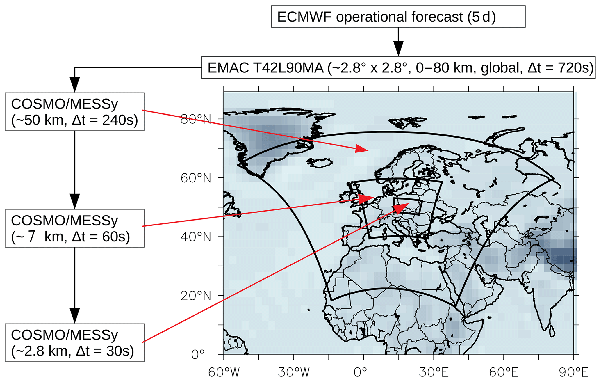
Figure 1 Overview of all three COSMO/MESSy domains over Europe (CM50), over central Europe (CM7) and over the USCB in Poland (CM2.8), as well as the corresponding temporal and spatial resolution. The black arrows indicate the data exchange between the different models. The driving model EMAC is nudged towards divergency, vorticity, temperature and the logarithm of surface pressure from the ECMWF. SST and SIC are prescribed as boundary conditions.

The second COSMO/MESSy instance (hereafter called CM7) covers the area over central Europe and is operated with a resolution of 0.0625^∘ (∼7 km) and a time step length of 60 s. The smallest instance (hereafter called CM2.8) covers the Upper Silesia in Poland and thus also the target region. CM2.8 has a resolution of 0.025^∘ (∼2.8 km) and a time step length of 30 s. The individual finer COSMO/MESSy instances (CM7 and CM2.8) are online driven from the respective coarser model domain (CM50 and CM7). In doing so, the respective coarser domain provides the boundary data for the smaller domain at each of its model time steps (EMAC: 720 s → CM50: 240 s → CM7: 60 s → CM2.8: 30 s). Figure 2 shows an overview of the initial and boundary data exchange between the different domains. CM50 and CM7 are operated with 40 vertical layers, and the smallest domain CM2.8 is operated with 50 vertical layers that cover the atmosphere from the surface up to an altitude of 22 km. A sponge zone begins at 11 km, which reaches the model top and nudges the model prognostic variables with increasing weights towards the driving model.

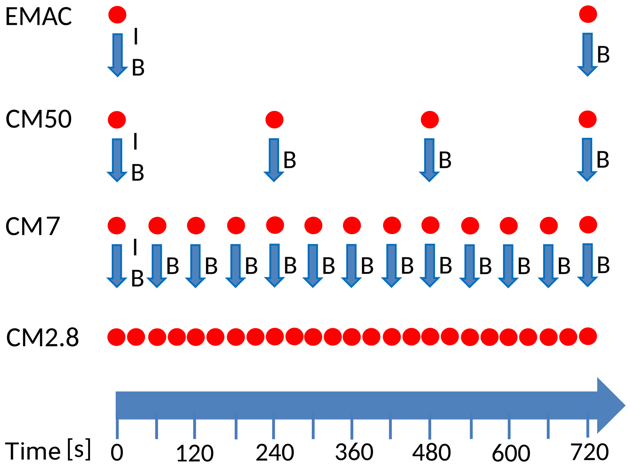
Figure 2 The illustration shows the initial and boundary data exchange between EMAC and the different COSMO/MESSy instances. The blue arrows symbolize the data exchange between the different model instances. B stands for boundary data and I for initial data. The red circles visualize the specific time steps of data exchange.

2.2.1 Methane tracers

CoMet aims to quantify the methane emissions in the USCB region, which actually arise from coal mining. In order to separate these emissions within our model, we define two different methane tracers. One tracer takes into account all methane emission fluxes (hereafter called CH4_FX) and includes the background methane, which is advected into the model domain. The second tracer (hereafter called PCH4) only considers the point source emissions of the ventilation shafts. In this way, we are able to trace back the methane enhancements of the first tracer CH4_FX (equivalent to what has been measured) to the coal mine emissions. Figure 3 shows an overview of both tracers, the involved submodels and the corresponding emission inventories. We initialize these two independent tracers for EMAC and for all three COSMO/MESSy instances equally. The initial conditions for the forecast simulations are derived from a continuous analysis simulation, which is described in detail in Sect. 2.3.

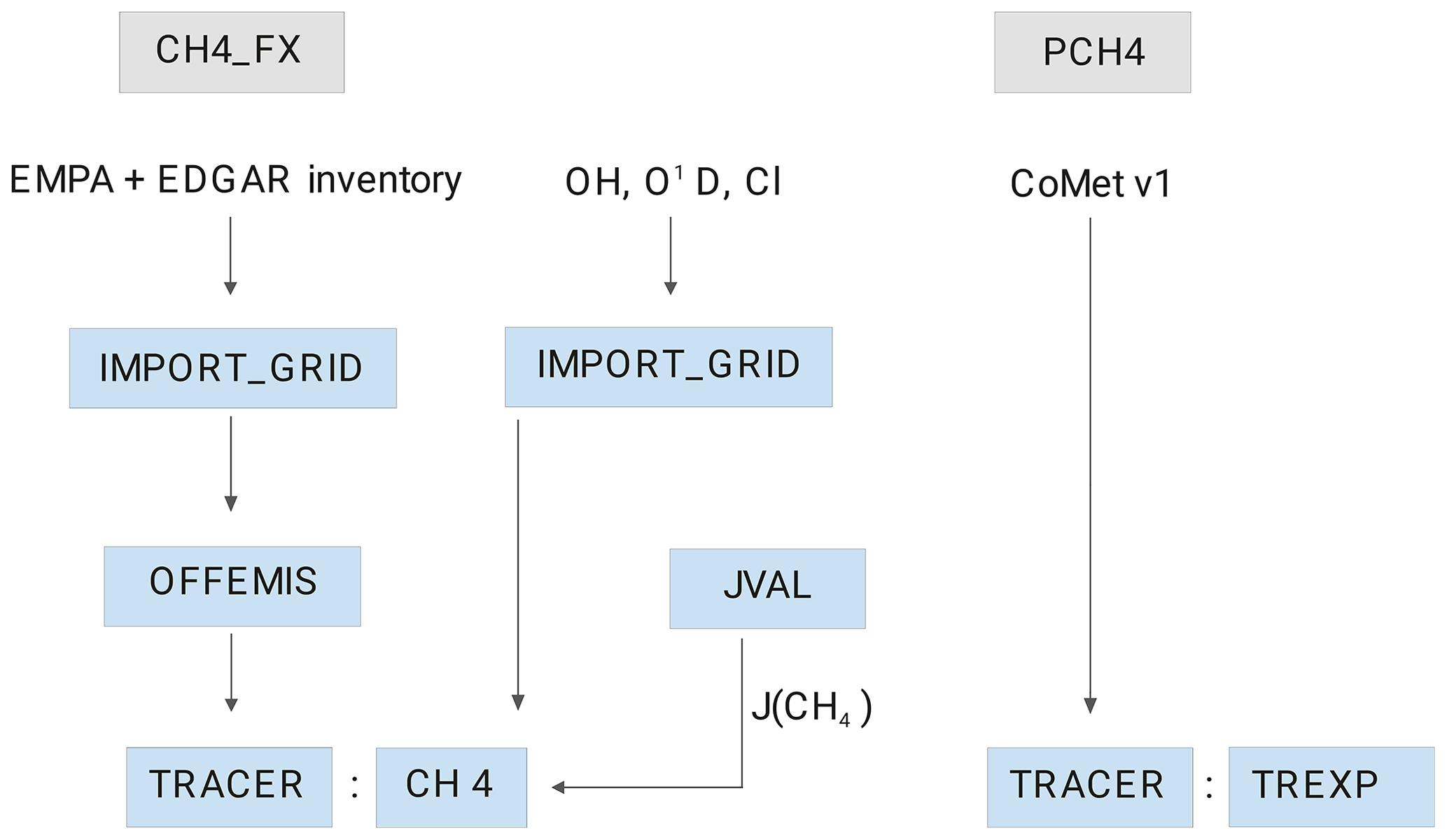
Figure 3 Illustration of the submodels which are used for the different methane tracers. CH4_FX tracer (left side): methane emission data and the oxidation reaction partners OH, O¹D and Cl are read from the NetCDF files and transformed to the computational grid by the submodel IMPORT_GRID. OFFEMIS converts the emission fluxes into tracer tendencies, and the CH4 submodel simulates the chemical loss of methane using the predefined fields of the oxidation partners and the calculated photolysis rate from the submodel JVAL. PCH4 (right side): the submodel TREXP is used for the point source emissions and tracer definition.

CH₄ point sources (PCH4)

The PCH4 tracer considers only point source emissions that are emitted by the ventilation shafts of the various coal mines in the USCB. In Fig. 4 the entire territory (49.90–50.40^∘ N latitude and 18.30^∘–19.40^∘ E longitude), together with the location of the ventilation shafts, is shown. To prescribe the emissions coming from the different shafts, we use CoMet ED v1, an inventory mainly based on the European Pollutant Release and Transfer Register (E-PRTR, 2014) but also on data from Wyzszy Urzad Gorniczy (2014). Further details on the names and exact positions of the different mines can be found in the Supplement. The total point source methane emissions in this area are estimated to be 465 kt a⁻¹ (CoMet ED v1 inventory). Emissions of single coal mines are split equally between the corresponding ventilation shafts. For the definition of point sources, we apply the MESSy submodel TREXP that is described in detail by Jöckel et al. (2010).

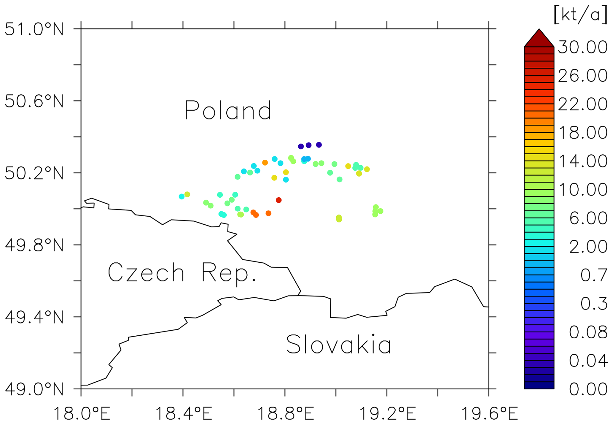
Figure 4 The map shows the locations and the emissions of methane in tons per year of the ventilation shafts in the USCB (CoMet ED v1). All ventilation shafts are gathered in the south-west of Poland close to the polish city Katowice and the Czech border.

Gridded methane emissions (CH4_FX)

The second tracer is called CH4_FX and includes all methane emission fluxes, anthropogenic and natural. We use an inventory which consists of two different parts, both monthly averaged: the year 2012 of the Swiss Federal Laboratories for Materials Science and Technology (EMPA) inventory (Frank, 2018) with a $\mathrm{1.0}{}^{\circ }\times \mathrm{1.0}{}^{\circ }$ grid resolution and the EDGAR v4.2FT2010 (2017) inventory with a finer grid resolution of $\mathrm{0.1}{}^{\circ }\times \mathrm{0.1}{}^{\circ }$. All anthropogenic (including rice cultivation) emissions are used from the EDGAR v4.2FT2010. Natural emissions and emissions caused by biomass burning are used from the EMPA inventory. The emission data are imported and transformed to the computational grid (IMPORT_GRID; Kerkweg and Jöckel, 2015). The emission fluxes are then converted into tendencies of the tracer CH4_FX (OFFEMIS; Kerkweg and Jöckel, 2012b, therein described as OFFLEM). Processes that are related to the methane chemistry in the model are described in the MESSy submodel CH4 (Frank, 2018). The submodel simulates the chemical loss of methane including the depletion by photolysis rate calculated by the submodel JVAL (Sander et al., 2014). The CH4 submodel uses predefined fields of the oxidation reaction partners OH, O¹D and Cl which, for our set-up, are derived as monthly averages (2007–2016) from a previous interactive chemistry simulation and read by IMPORT_GRID.

2.3 The forecast system

In order to achieve the best initial conditions of PCH4 and CH4_FX, the daily forecast simulations are branched from a continuous analysis simulation, which is essentially a hindcast simulation until the start of the forecast day. In the analysis simulation EMAC is nudged by Newtonian relaxation of temperature, vorticity, divergence and the logarithm of surface pressure towards the 6-hourly ECMWF operational analysis data. SST and SIC, derived from the same data set, are prescribed as boundary conditions for EMAC. The initial conditions of CH4_FX are derived as a monthly climatological average (2007–2016) of the simulation SC1SD-base-01, which is similar to the RC1SD-base-10 simulation (described in detail by Jöckel et al., 2016). PCH4 is initialized with zero. The starting date of the analysis simulations is 1 April 2018, which results in a spin-up time of 45 d. Nudging is applied in every model time step. The nudging fields (6-hourly data) and the prescribed SST and SIC (12-hourly data) are linearly interpolated in time. For this interpolation in time, starting and continuing the analysis simulation requires two nudging time steps ahead of the simulated time. An analysis simulation which should start at 00:00 UTC hence requires the nudging data of the time steps 06:00 and 12:00 UTC. Once the respective time period is simulated and the corresponding restart file is written, a new forecast simulation is triggered. The forecast branches as a restart from the analysis simulation and simulates a time period of 6 d by using the 6-hourly ECMWF operational forecast data for the EMAC nudging. PCH4 and CH4_FX are automatically initialized from the restart files. Throughout this process the analysis simulation continues. The forecast system is visualized schematically in Fig. 5. As soon as the preprocessed nudging files become available, the analysis simulation runs for about 50 min. Each forecast simulation takes about 8 h, and the post-processing takes another 1.5 to 2 h. The 8 h are for 144 message-passing interface (MPI) tasks on an Intel Xeon E5-2680v3-based Linux cluster (six nodes, each with 12 dual cores), whereby 6, 18, 56 and 64 tasks were used for the model instances EMAC CM50, CM7 and CM2.8, respectively. In our example, a forecast that simulates a time period starting at forecast day one at 00:00 UTC is readily post-processed on forecast day two at around 04:30 UTC (after approximately 28.5 h). Throughout both campaigns, forecasts were delivered every 12 h and made available online on a web page. In order to guarantee a continuous and uninterrupted supply of forecasts, we run the simulations alternately on two independent HPC (high-performance computing) clusters. An example of a forecast web product, which shows the forecast starting on 7 June 2019 at 00:00 UTC, can be found here: https://doi.org/10.5281/zenodo.3518926 (Jöckel et al., 2019). The post-processing includes the vertical integration of PCH4 and CH4_FX into a total-column dry-air average mixing ratio, called XPCH₄ and XCH₄ for PCH4 and CH4_FX, respectively. It is calculated as follows:

$$\begin{array}{}\text{(1)}& {\mathrm{XCH}}_{\mathrm{4}}={\displaystyle \frac{\sum \left({\mathit{\chi }}_{{\mathrm{CH}}_{\mathrm{4}}}\cdot m_{\mathrm{dry}}\right)}{\sum m_{\mathrm{dry}}}},\end{array}$$

where ${\mathit{\chi }}_{{\mathrm{CH}}_{\mathrm{4}}}$ is the methane mixing ratio, m_dry stands for the mass of dry air in a grid box and summation is carried out over all vertical levels. Figure 6 shows the design of XPCH₄ and XCH₄ which appeared on the forecast website. It is an example of a snapshot during CoMet 1.0 simulated with CM2.8.

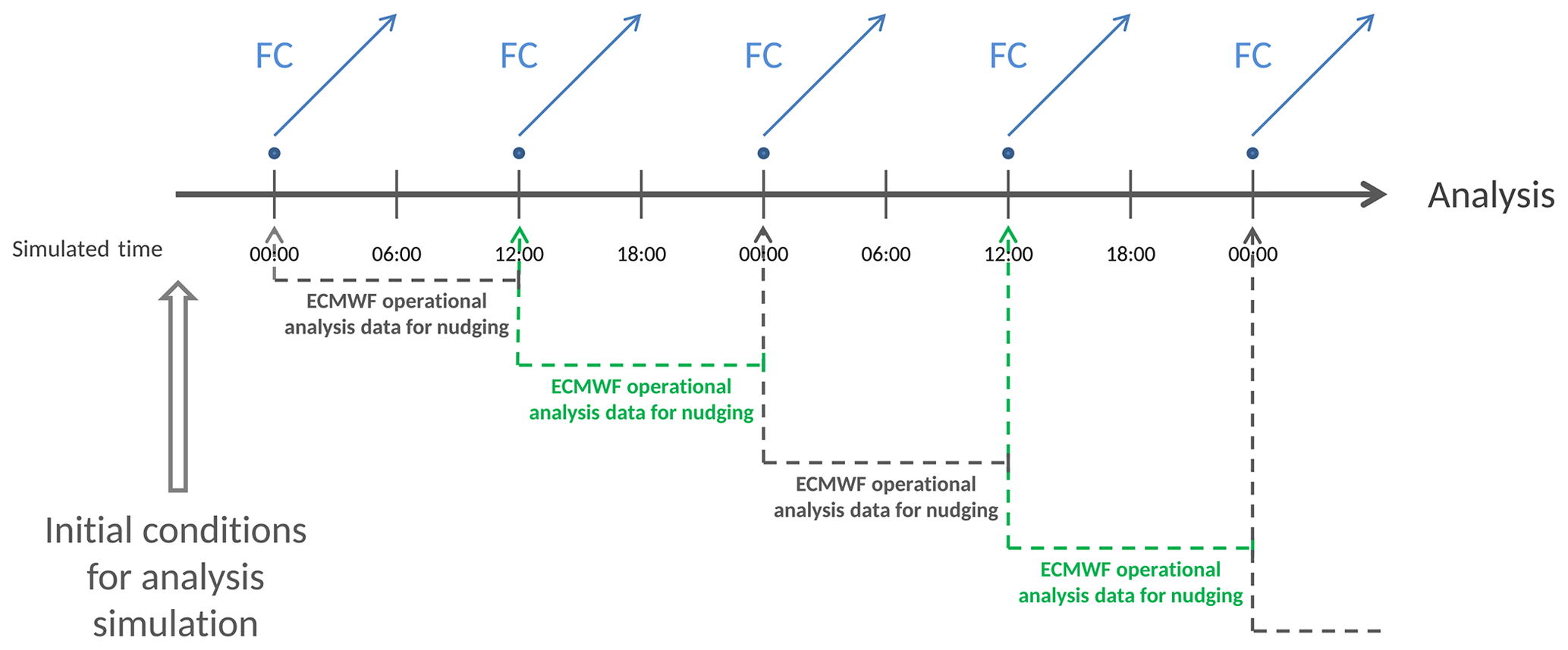
Figure 5 Chronology of the analysis simulation (dark grey) and the branching of the forecasts (FC, blue). The analysis simulation continues as soon as the ECMWF operational analysis data (two time steps ahead) are available for nudging. The required nudging time steps are indicated by the dotted lines in grey and green. A forecast simulation is branched (blue dots) every 12 h from the analysis at 00:00 or 12:00 and simulates a time period of 6 d. The initial conditions are provided by restart files of the analysis simulation.

3 Evaluation of analysis simulation

3.1 Observational data

During CoMet 1.0, methane was measured by active remote sensing. The instrument is an integrated-path differential absorption (IPDA) lidar called CHARM-F (Amediek et al., 2017), which was installed on board the German Research Aircraft HALO (High Altitude and LOng Range). CHARM-F was operated by the German Aerospace Center (DLR) in Oberpfaffenhofen and measured the weighted atmospheric columns of the methane dry-air mixing ratio from the surface to the flight altitude of the research aircraft. We compare our model results to the observations of the HALO D-ADLR flights on 6 and 7 June 2018. For simplicity, both data sets are hereafter called C1 and C2. See also Table 1, which lists all flights considered in this study and their abbreviations. Both data sets have a temporal resolution of 1 s and are already smoothed horizontally with a box window corresponding to 2 km of flight distance.

Table 1 Overview of the abbreviations for all observational methane data sets.

Additionally, methane was sampled in situ by cavity ring-down spectroscopy (CRDS). A JIG (Jena Instrument for Greenhouse Gases; Filges et al., 2015), which measured the methane mixing ratio in situ by CRDS, was installed on board HALO and operated by the Max Plank Institute for Biogeochemistry in Jena. Our model results are compared to the observations of the HALO flights on 6 and on 7 June 2018. Data sets are abbreviated as J1 or J2 (see Table 1). Both data sets have a temporal resolution of 1 s. A Picarro CRDS G1301-m instrument was installed on board the DLR research aircraft Cessna 208B (D-FDLR) and operated by the DLR in Oberpfaffenhofen. We compare seven flight observations to our model. Data sets are named accordingly as P1–P7 (see Table 1) and have a temporal resolution of 1 s.

Upon completion of CoMet 1.0, we conducted the analysis and forecast simulations again and used the specific geographical flight-track coordinates (degrees), pressure altitudes (hPa) and time steps (UTC) of all flights for the S4D submodel. The simulated data were then sampled as track-following curtains at each model time step, i.e. every 720 s, 240 s, 60 s and 30 s for EMAC, CM50, CM7 and CM2.8, respectively. However, our evaluation in this study only considers the two finest COSMO/MESSy instances CM7 and CM2.8. For the comparisons with the in situ observation, the curtain is further subsampled onto the flight altitude by linear interpolation. As the observed data have a finer temporal resolution than the model output, they are averaged over 60 s for CM7 and over 30 s for CM2.8. In order to compare our model results with those of the CHARM-F measurements, we calculate the dry-air mixing ratio between the surface and aircraft (in the following referred to as X_flCH4) using the S4D submodel output.

3.2 Comparison with analysis results

As the analysis simulation is nudged towards the ECMWF operational analysis data, we assume that this simulation reproduces the observed meteorology best. Thus, in order to find the best estimate of our model performance, the observations are compared to the analysis simulation results first. The model performance is analysed with respect to pattern similarity and amplitude, i.e. root mean square error (RMSE), standard deviation, correlation coefficient and normalized mean bias error (NMBE):

$$\begin{array}{}\text{(2)}& \mathrm{NMBE}={\displaystyle \frac{\sum \left({\mathit{\chi }}_{\mathrm{sim}}-{\mathit{\chi }}_{\mathrm{obs}}\right)}{n\cdot {\stackrel{\mathrm{‾}}{\mathit{\chi }}}_{\mathrm{obs}}}}\cdot \mathrm{100},\end{array}$$

where χ_sim is the simulated methane mixing ratio, χ_obs stands for the observed methane mixing ratio and the summation is over all n time steps. Compared to the observations, all CH4_FX model results are equally biased towards lower methane mixing ratios (see Figs. S2–S5 in the Supplement). The systematic bias is due to the lower background methane in the model. This is likely caused by the initialization from a monthly climatological average of a period between 2007 and 2016 (SC1SD-base-01; see Sect. 2.3), when global methane mixing ratios were lower than in 2018 (Nisbet et al., 2019). As OH is initialized from the same simulation (also as a monthly climatological mean) as methane, the OH field might also play a role. Yet, due to the short simulation period, this should not have a significant influence in our MECO(n) simulations. In order to evaluate the anomalies resulting from coal mine emissions rather than the discrepancies in background methane, we apply a bias correction to all model results involved in statistical comparisons with the in situ observations. For this purpose, we define an average bias of 0.108 µmol mol⁻¹ using the most frequently occurring difference between all D-FDLR in situ observations and the model results of instance CM2.8. Biases between CHARM-F and XCH4_FX are lower than the average offset of 0.108 µmol mol⁻¹, and it is difficult to determine a definite offset. Integration over a varying number of model levels or changes of topography, which are not resolved by the model, could be an explanation for this. The bias correction is therefore not applied to the vertically integrated values, which are compared to CHARM-F observations. The results are presented in Sect. 3.2.1 (CHARM-F) and Sect. 3.2.2 (D-FDLR and HALO in situ). In Sect. 3.2.3 we discuss all statistical results graphically.

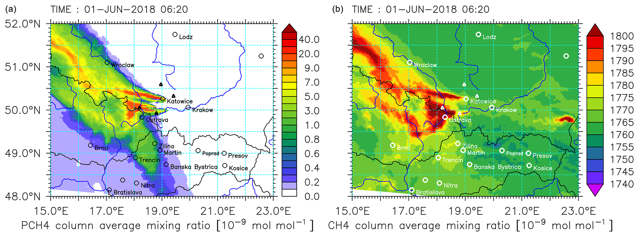
Figure 6 Snapshot of the methane forecasts during CoMet 1.0 simulated with the finest-resolved COSMO/MESSy instance CM2.8. The total-column dry-air average mixing ratio in micromoles per mole (µmol mol⁻¹) is calculated for PCH4 (a) and CH4_FX (b). The area encompasses the USCB and shows the evolution of methane plumes in the atmosphere. Note that the colour bar on the left is pseudo-logarithmic for better visualization.

3.2.1 Comparison with CHARM-F observations

Figure 7 shows the observed XCH₄ values of C1 and C2 as black lines. Red and blue dots display the simulated X_flCH₄ of CM7 and CM2.8, respectively, and all methane mixing ratios are given in micromoles per mole (µmol mol⁻¹). On both days the observed patterns agree well with the simulated patterns. Peaks in the observed methane mixing ratios are represented in CM7 and in CM2.8. From a visual point of view, amplitudes also appear to be similar. Mismatches can be seen on 6 June at around 09:30 UTC (see Fig. 7a) when model results are slightly shifted in time. Observed XCH₄ values follow a negative trend until 10:10 UTC, which is not simulated by the models. On 7 June the observed amplitudes are larger than those of the model results. On both days CM7 and CM2.8 do not differ significantly from each other. Furthermore, the comparisons reveal a continuous and constant bias. Simulated X_flCH₄ values are shifted towards smaller values compared to C1 and C2. Table 2 lists the root mean square error (RMSE; µmol mol⁻¹), the NMBE in percent and the correlation coefficient for all comparisons of the observations with the model results. NMBE is negative for all cases and ranges from −4.1 % to −5.3 %. NMBE and RMSE are lower for C1 (0.08 µmol mol⁻¹) than for C2 (0.10 µmol mol⁻¹), which confirms the assumption of higher mean amplitude similarity (standard deviation) on 6 June than on 7 June.

Table 2 Summary of the results of the statistical analysis of C1 and C2 compared to the simulated X_flCH4. Listed are the root mean square error (RMSE) in micromoles per mole (µmol mol⁻¹), the normalized mean bias error (NMBE) in percent and the correlation coefficient (R) for the model domains CM7 and CM2.8.

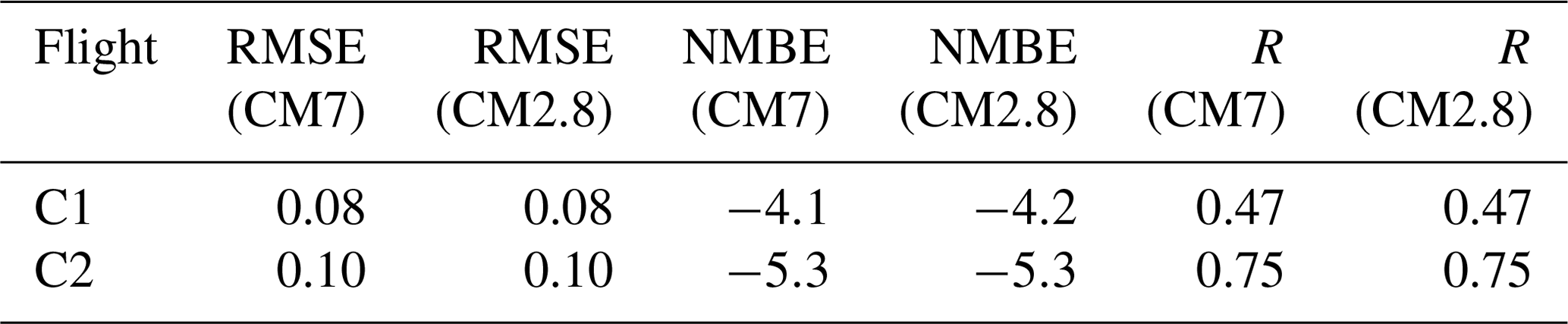
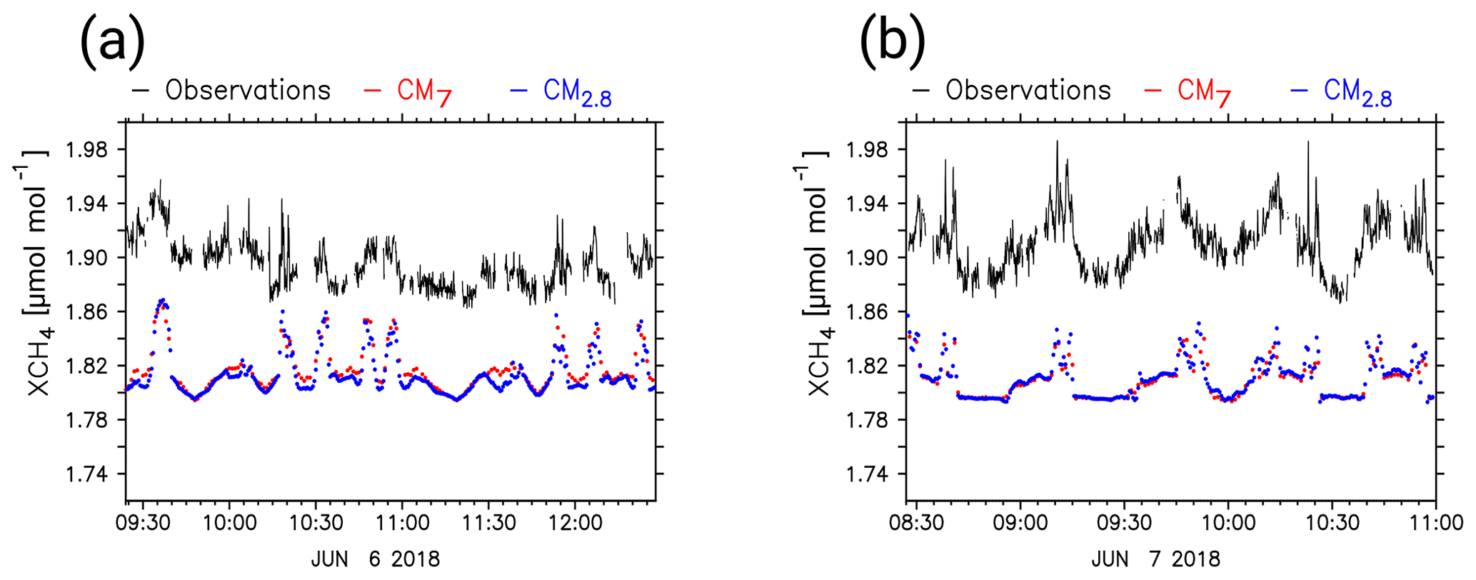
Figure 7 Results of the CHARM-F measurements and the S4D submodel sampling, which was vertically integrated to yield X_flCH4. XCH₄ values of C1 (a) and C2 (b) are displayed in black, and the simulated X_flCH₄ values of CM7 and CM2.8 are shown as red and blue dots, respectively. Mixing ratios are shown in micromoles per mole (µmol mol⁻¹). The time axes display the time of the specific flight in UTC.

3.2.2 Comparison with in situ measurements

Figure 8 shows the HALO in situ measurements of methane J1 and J2 in black, along with the simulated CH4_FX of CM7 and CM2.8 in red and blue, respectively. In addition, atmospheric pressure along the flight track is plotted in hectopascals (hPa) and indicates the changes in the flight altitude. The pressure follows a steep up-and-down movement between 900 and 200 hPa, which is because both flight paths were chosen to sample the vertical profile of methane in the atmosphere. The flight routes of J1 and J2 cover the USCB but also parts which are outside the smallest model domain (see Fig. 9). Gaps in the simulated CM2.8 mixing ratios mark the temporal leaving of the smallest area.

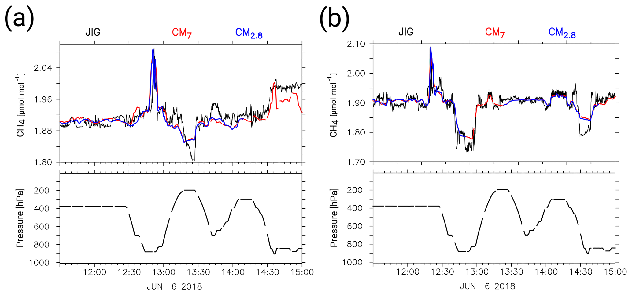
Figure 8 HALO in situ sampled methane mixing ratios (black lines) of J1 (a) and J2 (b), as well as the S4D submodel output at flight level for CM7 (red dots) and CM2.8 (blue dots). All mixing ratios are in micromoles per mole (µmol mol⁻¹), and the model results are bias-corrected. Below the methane mixing ratios, the atmospheric pressure along the flight track is shown in hectopascals (hPa). The time axis displays the time of the specific flight in UTC.

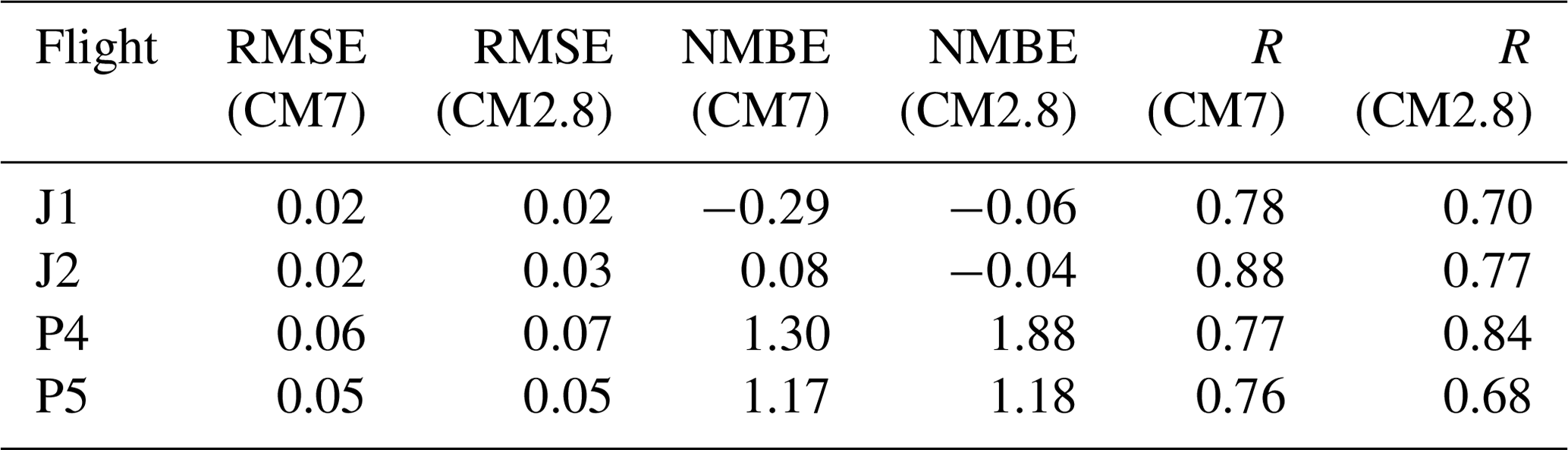
Overall, observed and simulated methane mixing ratios correlate closely with atmospheric pressure. Consequently, methane correlates negatively with flight altitude. Large-scale patterns and amplitudes are very similar in both model instances and in the observations. Table 3 lists the RMSE, NMBE and the correlation coefficient of J1 and J2 for the comparison with CM7 and CM2.8. NMBEs have similar values ranging from −0.29 % to 0.08 %. Although in very good agreement, the model is not able to simulate the small-scale fluctuations measured in the background methane at 400 hPa. Moreover, the model does not resolve the fine structure of the observations around 200 hPa. This can be seen in Fig. 8a at 13:20 UTC and in Fig. 8b at 12:00 and 14:30 UTC. As the mixing ratio at these altitudes is strongly influenced by the boundary conditions of the global model, we would not expect the model to be able to reproduce these features. In contrast, methane variability at lower altitudes is well represented in CM7 and CM2.8. In general, CM7 and CM2.8 are in good agreement. The RMSE for J1 is 0.02 µmol mol⁻¹ for CM7 and CM2.8. For the comparison with J2, the RMSE is similar with 0.02 µmol mol⁻¹ for CM7 and 0.03 µmol mol⁻¹ for CM2.8.

Table 3 Summary of the results of the statistical analysis of J1, J2, P4 and P5 compared to the simulated CH4_FX mixing ratios (bias-corrected). Listed are the root mean square error (RMSE) in micromoles per mole (µmol mol⁻¹), the normalized mean bias error (NMBE) in percent and the correlation coefficient (R) for the model domains CM7 and CM2.8.

Here, we discuss the D-FDLR flights P4, P5 and P2. All other D-FDLR observations and their comparison to the model results are shown in the Supplement. Figure 10 shows the comparison of the methane in situ measurements derived with the Picarro CRDS on board D-FDLR. The results shown are for the two flights P4 and P5. Both measurement flights aimed to sample the emissions of all methane sources within the USCB. The flight routes surround the USCB and follow a back-and-forth pattern along a horizontal track downwind of the mines, crossing the methane plume several times at different heights (see Fig. 11a and b). Figure 10a and b compare the simulated CH4_FX tracer mixing ratios along the flight tracks to the observations. Pattern similarity is good for both flights, and background methane shows little variability. Table 3 lists the respective RMSEs in micromoles per mole (µmol mol⁻¹), the NMBE in percent and the correlation coefficient for the comparison to both model instances of P4 and P5. On 6 June in the morning, the NMBE is 1.30 % for CM7 and 1.88 % for CM2.8. Peak mixing ratios of CM7 and CM2.8 reach values close to or higher than those of the observations, and around 10:15 UTC CM2.8 mixing ratios clearly exceed those of the observations. Although generally in good agreement, CM7 and CM2.8 differ from each other from 10:00 UTC to 10:30 UTC, when CM2.8 shows larger methane peaks than CM7. Regarding the afternoon flight (P5) model results again represent the observations well in terms of the time and location of the peaks. At 13:30 UTC the measured mixing ratios display a sharp increase, which is not distinctly presented in the model results. These high mixing ratios were taken very close to a specific coal mine, which is apparently not resolved well in CM2.8, and even less in CM7. In general, observed peaks during the afternoon flight are lower than those of the morning flight. This is also seen in the model results. Again, simulated methane peaks exceed the observational peaks but not as significantly, as seen for P4. The NMBE is consequently lower for P5, with 1.17 % and 1.18 % for CM7 and CM2.8, respectively.

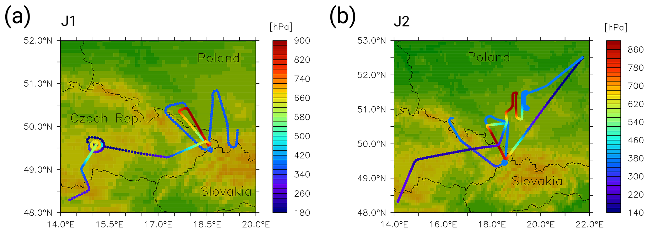
Figure 9 D-ADLR flight routes for J1 (a) and J2 (b). The colour bar refers to the atmospheric pressure at flight level.

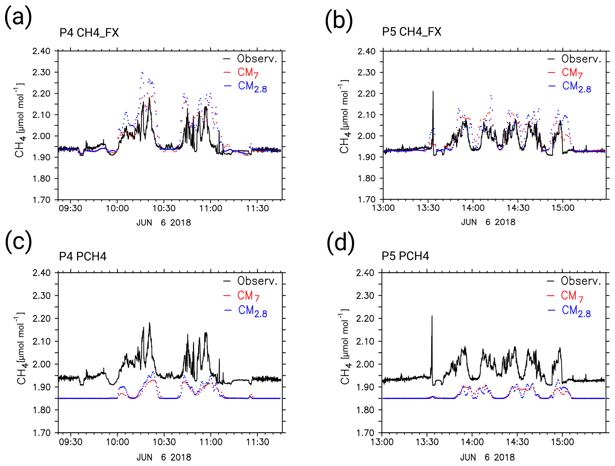
Figure 10 D-FDLR in situ sampled CH₄ mixing ratios (black lines) of P4 (a, c) and P5 (b, d), as well as the S4D submodel output at flight altitude for CM7 (red dots) and CM2.8 (blue dots). Panels (a) and (b) show the comparison with the CH4_FX tracer, whereas (c) and (d) show the comparison with the PCH4 tracer. All mixing ratios are in micromoles per mole (µmol mol⁻¹). CH4_FX is bias-corrected with 0.108 µmol mol⁻¹, and an offset of 1.85 µmol mol⁻¹ is added to PCH4 for a better visualization. The time axis displays the time of the specific flight in UTC.

Figure 10c and d show the comparison between the simulated PCH4 values along the flight track to P4 and P5. The black line illustrates the observed CH₄ mixing ratios micromoles per mole (µmol mol⁻¹), and the red and blue dots show the model results for CM7 and CM2.8, respectively. As PCH4 only considers the point source emissions without any background or other methane source emissions, one can assume that the enhancements seen in the model and in the measurements originate from the ventilation shafts. Smaller variations within the background methane are consequently not present in the model results and stay at a constant level of zero. To allow for a better comparison with the observations we added a constant offset of 1.85 µmol mol⁻¹ in both plots. The simulated PCH4 mixing ratios show a positive correlation with the major observed methane peaks. Although they have the same amplitudes, all methane elevations are simulated by the model. On 6 June in the morning, CM2.8 values exceed CM7 values and clearly show a more distinct structure. In the afternoon this difference is even more remarkable. CM2.8 is able to simulate the variability more precisely, whereas CM7 does not resolve the smaller patterns seen in the observations (e.g. at 14:30 UTC). The result for PCH4 contrasts with the CH4_FX tracer, for which peak emissions exceed the observations. We therefore compared the point source emissions of CoMet ED v1 to the anthropogenic emissions in the EDGAR v4.2FT2010 inventory. Whereas the point source emissions sum up to only 465 kt a⁻¹, the EDGAR v4.2FT2010 emissions, summed over all corresponding grid cells, are 1594 kt a⁻¹; 96.40 % of these emissions is attributed to the fugitive solid fuels of EDGAR sector 1B1.

Figure 11 D-FDLR flight pattern in the USCB for P4 (a, c) and P5 (b, d). Panels (a, b) show the vertical profile of the flight sections on 6 June 2018 between 10:10 and 11:20 UTC (a) and between 13:25 and 15:10 UTC (b). The colour bars refer to the bias-corrected CH4_FX mixing ratios in micromoles per mole (µmol mol⁻¹) simulated by CM2.8. Panels (c, d) show the flight routes in the USCB for P4 (c) and P5 (d). Here, the colour bars refer to the atmospheric pressure at flight level (hPa). Blue triangles show the locations of the coal mining ventilation shafts.

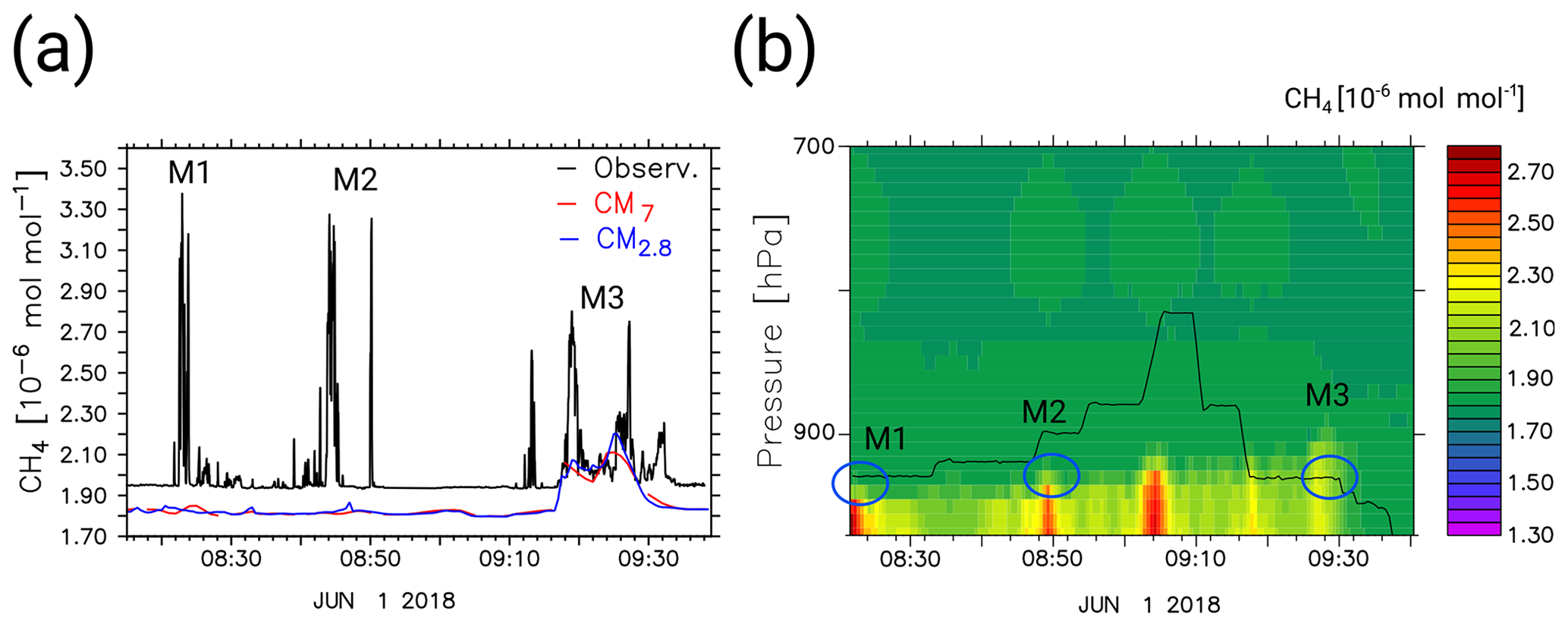
Figure 12 Panel (a) shows the D-FDLR in situ sampled CH₄ mixing ratios (black lines) of P2 and the S4D submodel output of CH4_FX at flight altitude for CM7 (red) and CM2.8 (blue). Panel (b) displays the corresponding flight altitude of P2 (black line) and the simulated profile (CM2.8) of the methane mixing ratio along this flight track. All mixing ratios are in micromoles per mole (µmol mol⁻¹). The time axes display the time of the flight in UTC. M1, M2 and M3 mark specific methane peaks seen in the observation (a) and in the simulated methane profile (b), but not necessarily in the sampled S4D output at flight altitude (a).

Figure 12a shows the comparison of the D-FDLR in situ observations of P2 on 1 June 2018 to the CH4_FX mixing ratios simulated by CM7 and CM2.8. Again, a systematic bias between observations and model results exists. Until 09:00 UTC atmospheric conditions were mostly stable and D-FDLR flew a back-and-forth pattern at a distance of 20 km downwind of the south-western cluster of USCB mines. The very high observed mixing ratios around 08:22, 08:45 and 08:50 UTC result from the only slightly diluted plumes. Those enhancements (M1 and M2) are barely detectable in the S4D output. The M3 enhancement was sampled further to the north, downwind of the northern USCB mines. Panel (b) shows the corresponding simulated (CM2.8) methane profile along a flight-track-following curtain and the flight altitude in black. The model results in panel (b) show elevated methane mixing ratios at M1 and M2. The methane peaks are below the top of the simulated planetary boundary layer height (PBLH) and below the flight track of P2. Consequently, they are not visible in the S4D results (panel a). These findings indicate that the simulated planetary boundary layer (PBL) during the morning is too low. In contrast, the observed methane peaks between 09:10 and 09:35 UTC (panel a) can be seen in the S4D results. Here, the PBL already extends towards higher altitudes and the flight track crosses the simulated methane plume (see panel b). Overall, CM7 and CM2.8 show smaller methane mixing ratios than observed.

3.2.3 Taylor diagram

Taylor diagrams combine three statistical metrics to better compare and interpret different model performances. They summarize the standard deviation (radial distance from the origin), correlation coefficient (angle) and centred RMSE (dashed semicircles) in a single diagram (Taylor, 2001). Thanks to the normalization of standard deviation and centred RMSE (NRMSE), metrics become non-dimensional and different model results can be compared to each other. The point on the horizontal axis displaying a normalized standard deviation of 1 outlines the point at which model results fit the observations perfectly. Figure 13 shows the results of the statistical analysis of CM7 (circles) and CM2.8 (triangles) compared to the observations (Table 1).

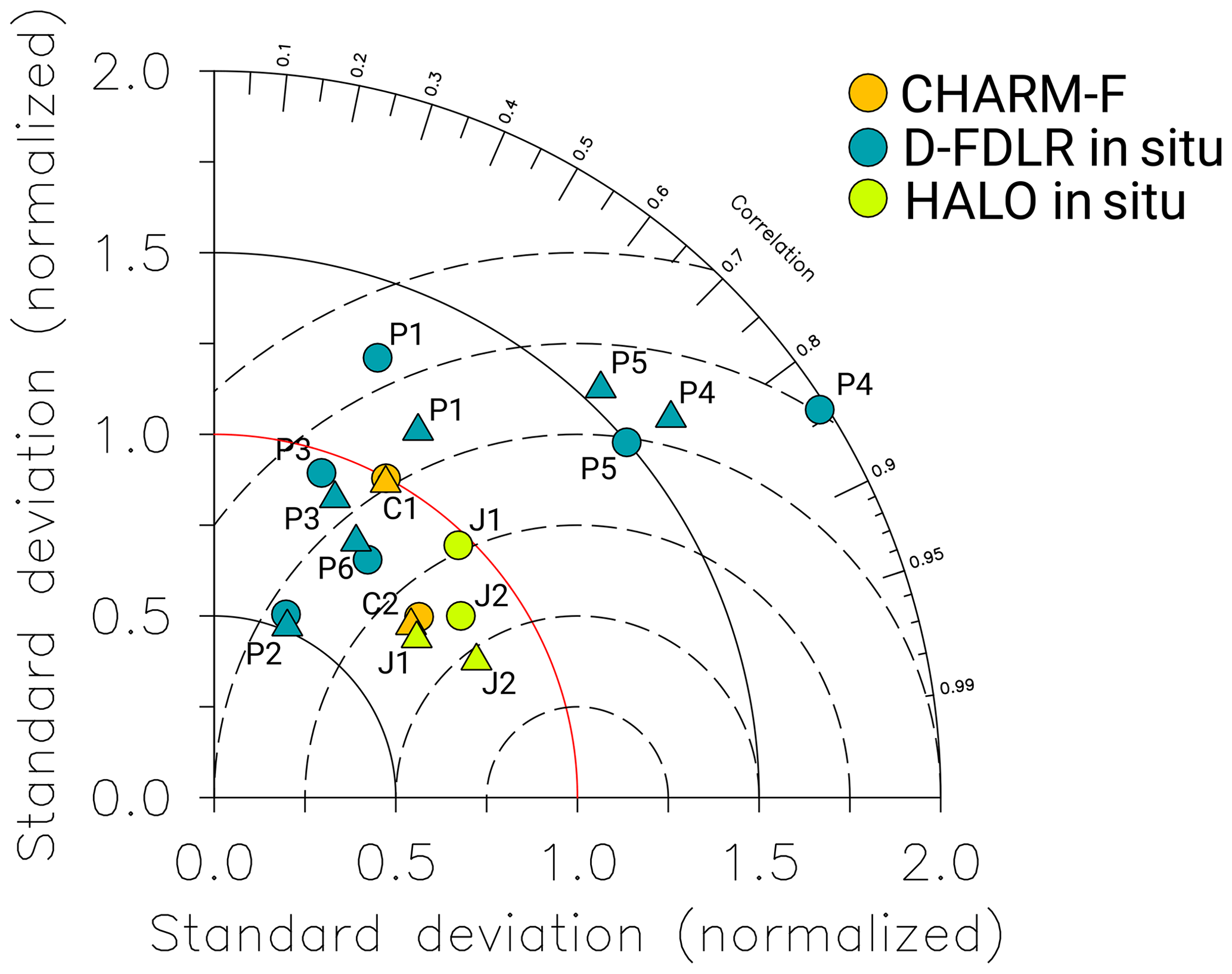
Figure 13 Taylor diagram summarizing normalized standard deviation (radius), correlation coefficient (angle) and centred NRMSE (dashed semicircles). Results show the comparison between observations and the model domain CM7 (triangles) and CM2.8 (circles). Comparisons to C1 and C2 are displayed in orange, those to P1 until P6 in blue and those to J1 and J2 in green. P7 is outside the diagram.

The three data sets differ in measuring technique and in their geographical extent, duration and daytime of sampling. This makes it difficult to define an overall model skill. The meteorological situation, such as wind conditions or convection, and topographical features may lead to further uncertainties. The comparison to J1 and J2 is the best in the Taylor diagram. Results are close to the reference point on the horizontal axis (normalized standard deviation 1.0) and correlation coefficients are very high, especially for CM7. The measurements cover larger areas outside the USCB including, for example, the Czech Republic. Other than for C and P observations, the horizontal distribution of the methane plumes only plays a minor role. The JIG samples focus on the vertical gradient of methane in the atmosphere, which is well represented in the model (Fig. S1 in the Supplement). The comparisons to C are also reasonably good. The C1 pattern statistically differs from the observations, which may be due to a temporal or spatial shift of the plume in the model at the beginning of 6 June. But normalized standard deviations are close to 1, and CM7 and CM2.8 agree equally with the observations. Since CHARM-F measures the total-column average mixing ratio, mismatches between actual and simulated PBLH are less apparent. The comparisons to the smaller-scale P observations assess the model ability to represent regional-scale features like coal mine emission plumes. As described in Sect. 3.2.2, the skill also depends on how well the model actually simulates the PBLH. We can further see the highest variability between CM2.8 and CM7 for the comparisons with P. Depending on the grid size of the model, the very localized methane enhancements can be either more diluted or more intensified in the model results. And mixing ratios sampled very close to the ventilation shafts are often not resolved by the model. Furthermore, high wind speeds, for example during the sampling of P7 (see the Supplement), lead to a low correlation with MECO(n) and a normalized standard deviation larger than 2. P7 is consequently not present in the Taylor diagram. Finally, C and J data were sampled on 6 and 7 June when wind conditions were stable. Additional data would be necessary in order to compare the models' skill on days with less perfect conditions, such as for P.

4 Evaluation of forecast skill

A good forecast should be able to simulate both the amplitude and pattern variability of the observed methane mixing ratios in the atmosphere. To identify the temporal evolution of the forecast skill with each forecast day, we therefore calculate skill scores (after Taylor, 2001) that consider standard deviation and correlation coefficient. We used the two different skill scores

$$\begin{array}{}\text{(3)}& S_{\mathrm{V}}={\displaystyle \frac{\mathrm{4}(\mathrm{1}+R)}{({\mathit{\sigma }}_{\mathrm{f}}+\mathrm{1}/{\mathit{\sigma }}_{\mathrm{f}}{)}^{\mathrm{2}}(\mathrm{1}+R_{\mathrm{0}})}}\end{array}$$

and

$$\begin{array}{}\text{(4)}& S_{\mathrm{C}}={\displaystyle \frac{\mathrm{4}(\mathrm{1}+R{)}^{\mathrm{4}}}{({\mathit{\sigma }}_{\mathrm{f}}+\mathrm{1}/{\mathit{\sigma }}_{\mathrm{f}}{)}^{\mathrm{2}}(\mathrm{1}+R_{\mathrm{0}}{)}^{\mathrm{4}}}},\end{array}$$

which either emphasize the similarity of the amplitudes or the similarity of the patterns. R is the correlation coefficient between the forecast and observation, R₀ is the maximum attainable correlation coefficient, and σ_f is the ratio of the standard deviation of the forecast to that of the observation. We assume R₀ to be 1, although in reality maximum correlation coefficients between observations and simulations cannot be reached due to differences in spatial and temporal resolution. The skill ranges between 0 and 1, with small values indicating low skill and high values indicating high skill. We use the analysis simulation as a reference observation to evaluate a theoretical forecast skill. As the forecasts are branched from the analysis simulation we aim to quantify the deviation of the forecast from the analysis with increasing forecast day. The results are discussed in Sect. 4.1. In order to find the actual skill of the forecast, we further compare the different forecast days to the observations C1, C2, J1, J2, P4 and P5. Section 4.2 describes these results.

4.1 Theoretical forecast skill

We compare every single forecast day out of six forecast days to the analysis simulation (between 1 and 22 June 2018) and calculate a daily skill score at each point on the respective two-dimensional model grid. The skill is calculated for the simulated CH4_FX values. In order to compare CM7 and CM2.8, the analysed area only covers the area obtained by removing the outermost 15 grid points of the CM2.8 domain (relaxation area). Figure 14 assigns to each forecast day the average percentage of the area which reveals a skill score larger than 0.7. The results are shown in red for CM7 and in blue for CM2.8. Panels (a) and (b) refer to the different skill scores S_V and S_C, respectively.

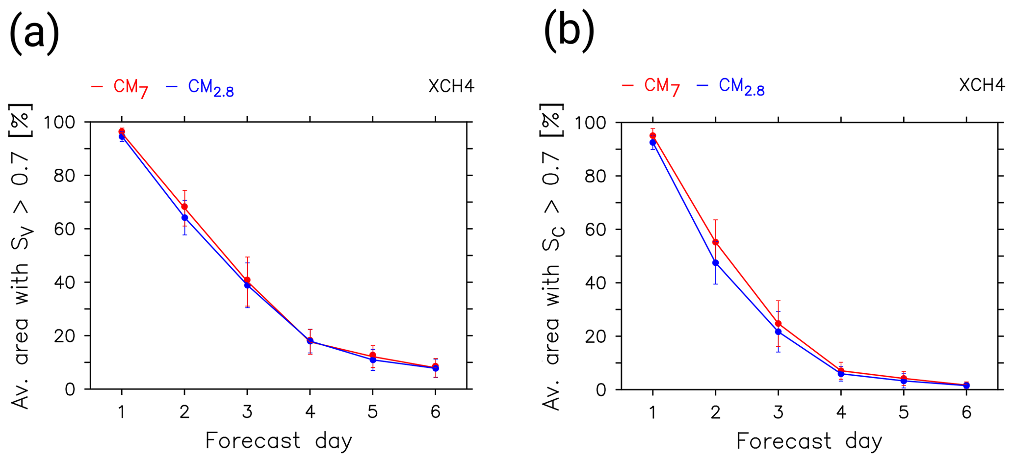
Figure 14 The graphic shows the evolution of the theoretical forecast skill with increasing forecast day for CM7 (red) and CM2.8 (blue). The vertical axis displays the average area (%), according to the smallest model domain, with a skill score >0.7. The horizontal axis shows the specific forecast days one to six. The skill scores are calculated for each day at each grid point from 1 to 22 June 2018 (CoMet 1.0). The CH4_FX total-column mixing ratios of the forecast simulations are compared to the CH4_FX total-column mixing ratios of the analysis simulation. The error bars indicate the interval which contains 95% of all skill scores per day. S_V (a) emphasizes variability and S_C (b) emphasizes the correlation.

On forecast days one to three, CM7 shows slightly larger values than CM2.8. This is most obvious for S_C, which puts greater emphasis on the correlation coefficient. However, differences between the two model instances are rather small. The forecast skill is very large at forecast day one. Here, the forecasts are branched from the analysis simulation, which results in good agreement between the reference and forecast. Both skills decrease with increasing forecast day, and the skill in Fig. 14b shows a steeper decrease than the skill in Fig. 14a. This suggests that the correlation between the forecast and analysis is reduced faster than the similarity of amplitudes. For S_V, the area which exceeds a threshold of 0.7 covers about 65 % and 40 % at forecast days two and three, whereas for S_C it only covers about 50 % and 25 %, respectively. From forecast day four onwards, less than 20 % (S_V) or 10 % (S_C) of the area reveals a skill larger than 0.7. The lower correlation could be attributed to a displacement of the simulated plume in time or space, which would also explain the fact that the normalized standard deviation remains within the given range.

4.2 Actual forecast skill

Figure 15 shows the skill score S_V calculated for the different forecast days one to six when compared to the observations C1, C2, J1 and J2 (see panel a) and to the observations P1–P7 (see panel b). Results for CM7 and CM2.8 are shown on the left and right side, respectively. In contrast to the theoretical skill, for which S_V and S_C clearly decrease with increasing forecast day, a reduction of the skill is not obvious here. Whereas the theoretical skill score is defined to measure the skill averaged over the entire model domain, the actual skill score compares the model results to observational data. The latter measure the downwind methane plumes, which are easier to forecast than the variability of the methane background in the overall model domain. Considering the difference between the single observations, S_V is highest for J1 and J2 with values above 0.8. They are followed by C1 and C2 with values above 0.65 (except for C1 on forecast day one) and P1, P4, P5 and P6 mainly showing a skill between 0.6 and 0.8. The skill is lowest for the comparison with P2 and P7. S_V emphasizes the similarity of amplitude between the forecast and observation. This similarity seems to be highest with HALO in situ and CHARM-F observations. As already discussed in Sect. 3.2.3, the models' skill differs between the three data sets, which is mainly due to different flight patterns and measurement techniques. J and C observations measure larger-scale vertical and integrated horizontal distributions of methane, respectively. Both are well represented in MECO(n). Modelling the smaller-scale features observed by P is, however, challenging, which is also reflected in the comparison with the forecasts. S_V does not vary significantly among the different forecast days nor does it show any specific trend. Results for C1, P4, P5 and P7 drop at forecast day five but increase again at forecast day six. In contrast, P2 suddenly increases at forecast day five. Differences between CM7 and CM2.8 are rather small. Figure 16 summarizes the results of the skill score S_C. S_C is generally lower than S_V, which is due to higher weighting of the correlation coefficient. Overall, the skill is best for J1, J2, C2, P4 and P5, meaning that the model and observations correlate well here. As mentioned in Sect. 3.2.3, conditions for measuring the downwind methane plumes on these days were favourable and model results agree better with the observations. In contrast, P2 and P7 again show very low values (see also Fig. 15). In panel (a), CM7 and CM2.8 show a similar pattern. The skill among the different forecast days almost stays at the same level or even increases until forecast day four. Forecast days five and six show lower skill, with the lowest values for C1 at forecast day five. The skill for J1 and J2 shows generally lower values in CM2.8 than in CM7. In panel (b) the skill is highly variable among all forecast days until day four. On forecast days five and six, skill decreases for all comparisons, with very low values for P7.

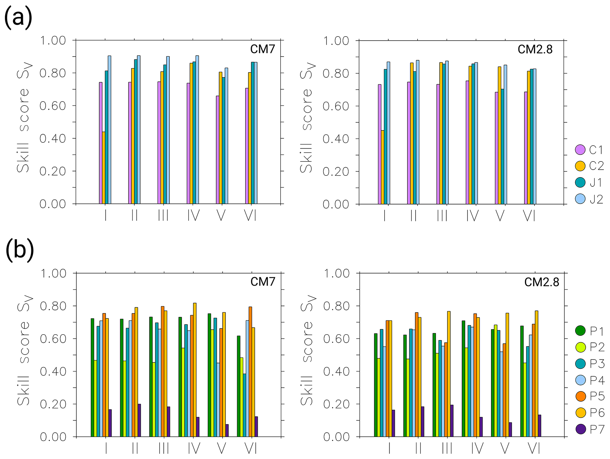
Figure 15 The bar plots show the calculated skill scores S_V for the comparison of forecast days one to six (horizontal axis) to the observations. The colours refer to the different observations. Panel (a) displays the results for C1, C2, J1 and J2. Panel (b) shows the results for P1–P7. The CM7 and CM2.8 results are shown on the left and right side, respectively.

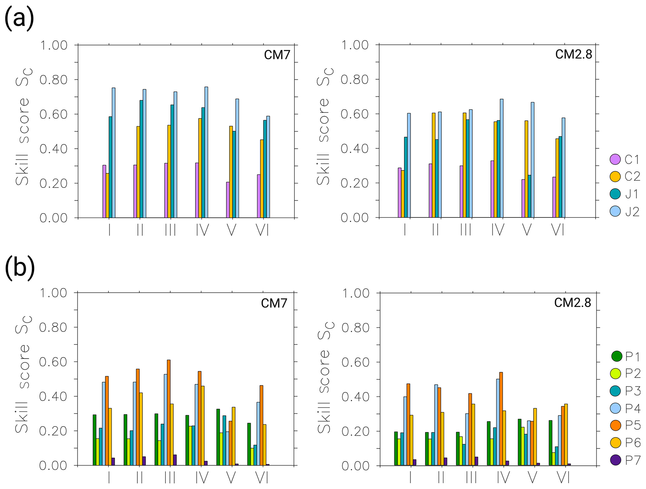
Figure 16 The bar plots show the calculated skill scores S_C for the comparison of forecast days one to six (horizontal axis) to the observations. The colours refer to the different observations. Panel (a) displays the results for C1, C2, J1 and J2. Panel (b) shows the results for P1–P7. The CM7 and CM2.8 results are shown on the left and right side, respectively.

5 Discussion

Overall, the comparison of the analysis simulation with airborne-derived measurements shows that MECO(n) is able to simulate the observed methane plumes reasonably well. This is the intended result considering that EMAC is nudged towards the ECMWF data at a coarser resolution (T42 spectral truncation), and CM50, CM7 and CM2.8 are nested into each other and only driven by relaxation at their boundaries by the next coarser model instance. Nevertheless, a continuous and constant offset of the simulated CH4_FX to all observations results from all model instances. As the bias is constant at all altitudes, it is most likely not caused by shortcomings in the vertical transport in the model. Instead, a global increase in methane emissions (Nisbet et al., 2019) could explain the discrepancy between the observations and the model results that are based on EDGAR v4.2FT2010 for anthropogenic emissions and on the EMPA inventory (Frank, 2018) for all other emissions fluxes. Apart from that, the timing of the simulated peaks is in good agreement for all observations. Compared to CHARM-F observations, the simulated X_flCH₄ peaks show similar or slightly lower amplitudes. The vertical methane gradient measured by the JIG is well represented by MECO(n). Besides the smaller variations in the background methane, the model results correlate well with the measured methane mixing ratios at different altitudes. By comparing the small-scale D-FDLR in situ measurements, the simulated amplitude of the peaks is mostly overestimated. This particularly applies for the CM2.8 results. Anthropogenic emissions in the EDGAR v4.2FT2010 inventory differ from the latest release of EDGAR v4.3.2 (2019). Total anthropogenic methane emissions for the USCB (here: long. 18.30–19.40^∘ E, lat. 49.90–50.40^∘ N) are 1636 kt a⁻¹ in EDGAR v4.2FT2010 and only 605.6 kt a⁻¹ in EDGAR v4.3.2. The overestimation of local methane plumes in the model can therefore be explained by the overestimation of methane emissions in EDGAR v.4.2FT2010. However, we also see high peaks in the methane mixing ratios of the D-FDLR in situ observations, which are very low in the model results or not present at all. This is mainly the case when D-FDLR sampled very close to the ventilation shafts (see results for P3 in the Supplement). Here, the model cannot resolve the very localized enhancements. Larger grid sizes lead to instantaneous dilution of the simulated mixing ratios close to the ventilation shafts. Or, as seen for 2 June 2018, the simulated PBL is too shallow and lies below the flight altitude. Consequently, the enhanced methane mixing ratios are not present in the S4D results along the flight track at flight altitude. Previous studies (i.e. Collaud Coen et al., 2014; Mertens et al., 2016) analysing the simulated PBLH of the COSMO model show results that oppose our findings. However, this is just a snapshot of a short-term simulation and our study does not provide a detailed analysis of the PBL. Additionally, PCH4, which only considers the emissions of the ventilation shafts, is in good agreement with the CH4_FX tracer and the observed methane elevations. This indicates that the observed methane plumes actually originate from coal mining. Although the assessment of the single point source emissions is not part of the current study, it should be noted that the different PCH4 point sources can be switched on and off in the model individually. This provides a good tool to distinguish between different sources and to assign them to the different measurements. When compared to the small-scale D-FDLR in situ measurements, PCH4 correlates well with the observed methane mixing ratios. In contrast to the CH4_FX results, the point source tracer does not overestimate the emissions. However, it also does not show the same emission strength as the observations. PCH4 peaks have considerably lower amplitudes than observed. The reason for this discrepancy is the different emission inventories for CH4_FX and PCH4. The sum of all methane emissions in CoMet ED v1 used for PCH4 is 465 kt a⁻¹, which is less than a third of the EDGAR v4.2FT2010 emissions (summed over the corresponding grid boxes). Updated estimates of emissions from CoMet ED v2 (based on E-PRTR, 2016) indicated larger emissions of 502 kt a⁻¹ and some changes in the distribution of emissions, following structural and operational changes in the mining sector over the period between reporting years (2014 and 2016 for CoMet ED v1 and v2, respectively). This implies that the simulated PCH4 using the latest emission inventory CoMet ED v2 is expected to match the observed amplitudes better. Another reason for the underestimation of the simulated PCH4 peaks might be the fact that we assume a temporally constant methane release from the ventilation shafts. But in reality the emitted amount of methane varies from day to day. This might have a small influence on the results but would not explain the large differences between PCH4 and the observations. Overall, CM7 is able to simulate the large-scale observations (HALO in situ) and the vertically integrated methane (CHARM-F) as precisely as CM2.8. When compared to small-scale measurements (D-FDLR in situ) the model overestimates the observed peaks. This is especially true for the finer-resolved CM2.8, whereby methane mixing ratios are larger than the mixing ratios simulated by CM7. Smaller grid cells may catch locally enhanced methane mixing ratios in the plume, whereas coarser grid cells cover a larger portion of the methane plume and mixing ratios may be more diluted. Additionally, CM2.8 is able to better simulate the fine structure of the small-scale observations. However, the differences are rather small and the observed methane peaks are well represented in both model instances.

The theoretical forecast skill illustrates the deviation of the forecast from the analysis simulation. Results show a decreasing trend with increasing forecast day. Nevertheless, the correlation and amplitude similarities of a single forecast day show a broad variation. The evaluation of the actual forecast skill reveals even less clear results. The amplitudes seem to be constant or at least do not show any specific trend with increasing forecast day, but the correlation between the observation and forecast slightly decreases. Forecast day five seems to yield the lowest skill for P4 and P5 and also for C1 and J1, which is less obvious than for P4 and P5. Due to the fact that these observations were sampled during only 1 d, namely 6 June 2018 in the morning and in the afternoon, all comparisons for the fifth forecast day are related to the forecast simulation start date on 2 June. Disagreement may be due to the specific meteorological situation of this day. In order to make a general statement about the forecast skill, it would be necessary to compare additional observations within a broader time span.

We successfully conducted 6 d forecast simulations of methane with the online coupled, three-time nested global and regional chemistry–climate model system MECO(3). The forecasts branch from a continuous analysis simulation, in which EMAC is nudged towards the operational ECMWF analysis data. This is essential for appropriate initial forecast conditions. We continuously delivered the forecasts during CoMet 1.0 and analysed the model and forecast performance with respect to the observations. The advantage of using the global–regional model system is that we are able to simulate both the point source emissions and the background methane. For the latter, it is essential to provide lateral boundary conditions to the nested model instances which are consistent with the meteorology, i.e. the dynamical boundary conditions. This makes it possible to distinguish between local source emissions and fluctuations in the background methane, which is important for the quantification of different methane sources. Even though the data for Newtonian relaxation are first coarsened to a horizontal grid resolution corresponding to the T42 spectral truncation and then nested three times down to a spatial resolution of 2.8 km, MECO(3) is able to simulate the observed methane plumes correctly. Overall, the vertically integrated values, e.g. total-column average mixing ratios, and the large-scale patterns, such as the vertical gradient of methane, are well represented. However, limitations exist for the simulation of small-scale patterns. A bias reduction and better agreement of small-scale simulated methane amplitudes with the observations may be achieved by updating the applied emission inventories to the EDGAR v4.3.2 inventory for anthropogenic emissions and the latest information on point source emissions (CoMet ED v2). Another anthropogenic emission inventory, which could reduce the bias, is the CAMS-GLOB-ANT inventory (Granier et al., 2019). CAMS-GLOB-ANT extrapolates the emissions to the current year by using EDGAR v4.3.2 as a basis for 2010 and by projecting emission trends for 2011 to 2014 from the Community Emissions Data System (CEDS) inventory (Hoesly et al., 2018) until 2018. Furthermore, we obtained decent results up to forecast day four. The skill score calculated for all forecast days is reasonable. However, due to the limited number of comparable observations, the skill score might not be representative and its interpretation must be treated with caution. All observed methane peaks are well represented in both model domains CM2.8 and CM7. For the purpose of the field campaign, it is therefore sufficient to perform the forecasts with CM7 only.