Similarities within a multi-model ensemble: functional data analysis framework

Despite the abundance of available global climate model (GCM) and regional climate model (RCM) outputs, their use for evaluation of past and future climate change is often complicated by substantial differences between individual simulations and the resulting uncertainties. In this study, we present a methodological framework for the analysis of multi-model ensembles based on a functional data analysis approach. A set of two metrics that generalize the concept of similarity based on the behavior of entire simulated climatic time series, encompassing both past and future periods, is introduced. To our knowledge, our method is the first to quantitatively assess similarities between model simulations based on the temporal evolution of simulated values. To evaluate mutual distances of the time series, we used two semimetrics based on Euclidean distances between the simulated trajectories and based on differences in their first derivatives. Further, we introduce an innovative way of visualizing climate model similarities based on a network spatialization algorithm. Using the layout graphs, the data are ordered on a two-dimensional plane which enables an unambiguous interpretation of the results. The method is demonstrated using two illustrative cases of air temperature over the British Isles (BI) and precipitation in central Europe, simulated by an ensemble of EURO-CORDEX RCMs and their driving GCMs over the 1971–2098 period. In addition to the sample results, interpretational aspects of the applied methodology and its possible extensions are also discussed.

1 Introduction

While numerical climate models serve as the cardinal tool of contemporary climatology, their outputs are typically burdened by distinct uncertainties, manifesting through substantial differences between individual simulations. Here, we address the issue of comparing various climate simulations and quantifying their differences by introducing a methodology for analysis of multi-model ensembles and the relationship between nested regional climate model simulation and its driving global climate model (GCM) run. We propose use of a metric generalizing the concept of similarity, based on the information contained in the entire simulated climate series, extending from historical to future periods. The evaluation framework is based on functional data analysis (further denoted as FDA; Ramsay and Silverman, 2005, 2007; Ferraty and Vieu, 2006).

The analysis of uncertainties in climate model outputs is a key research topic, especially due to the use of model simulations as inputs for studies of possible future climate change impacts. The results of the respective analyses serve as the basis for important adaptation and mitigation decisions, with a critical role belonging to the information on reliability of the projections and the structure of the relevant uncertainties. Climate model outputs are subject to uncertainties coming from various sources, including imperfect initial and boundary conditions, parameterizations of small scale processes, or necessary choices and simplifications in the model structure (numerical schemes, spatial resolution, etc.). For detailed discussion, see, for example, Tebaldi and Knutti (2007). When considering regional climate models (RCMs), it is necessary to take into account some additional factors, mainly connected to the limited integration domain (Laprise et al., 2008) or possible inconsistencies of parameterization schemes between driving and nested models (Denis et al., 2002). The estimate of the uncertainties in climate model outputs must accompany any future climate change scenario.

One of the most frequently used ways of uncertainty assessment is the analysis of multi-model ensemble (MME) spread (e.g., Belda et al., 2017; Holtanová et al., 2010; Prein et al., 2011). The main aim of MMEs is to sample the uncertainty stemming from choices in model structure, parameterization schemes and, in the case of RCMs, also boundary conditions. Estimating the uncertainty range based on the MME spread is not a straightforward task, as currently available MMEs suffer from various deficiencies. One obstacle is raised by the deficiencies in the statistical experimental design: models are developed voluntarily from institutions worldwide. This problem is further amplified when designing an ensemble of RCMs. An RCM is driven by a GCM, which has a substantial effect on the nested simulation (Déqué et al., 2007, 2012; Heinrich et al., 2014). It is not computationally feasible to run all combinations of RCMs with every GCM. Therefore, for a proper uncertainty assessment it is crucial to investigate the interactions between driving GCMs and nested RCMs and their respective influence on the total MME spread (e.g., Déqué et al., 2012; Holtanová et al., 2014; Heinrich et al., 2014; Holtanová and Mikšovský, 2016).

In addition, climate models (even across developing institutions) are known to share certain components, leading to inter-model similarities and dependencies. This makes it difficult to justify the independence assumption when quantifying the uncertainty of MMEs with standard statistical models. Recently, innovative methods have been developed to identify groups of similar climate models (e.g., Knutti et al., 2013) and account for the similarities (Annan and Hargreaves, 2017). However, these methods quantify model similarity based on either their behavior in approximating the historical climate or purely on their projected climate change signals. Some studies included evaluation of the relationship between the driving GCM and nested RCM based on more advanced climatic characteristics (e.g., Rajczak and Schär, 2017; Crhová and Holtanová, 2018), but their approach to the issue was rather qualitative. To our knowledge, our method is the first to quantitatively assess similarities between model simulations based on the temporal evolution of simulated values.

To illustrate a possible application of the proposed methodology we analyze similarities and dissimilarities between members of the EURO-CORDEX multi-model ensemble (Jacob et al., 2013) and their driving GCMs. The inter-model distances between the trajectories of the temporal development of running 30-year mean changes in seasonal mean air temperature and precipitation are evaluated. We first assessed the similarities between ensemble members for time series averaged over eight large European regions defined by Christensen and Christensen (2007) that have been widely used for climate model assessments (e.g., Rajczak and Schär, 2017; Holtanová and Mikšovský, 2016; Mendlik and Gobiet, 2016). Here we show the results for only two chosen cases, namely the winter mean air temperature over the British Isles (BI) and mean summer precipitation over eastern Europe (EA). These two cases were chosen to illustrate two distinct cases of GCM–RCM interaction.

The paper is structured as follows. In Sect. 2 the EURO-CORDEX regional climate models and their driving global climate models are briefly introduced. In Sect. 3 the methodology is described, including the basic information about the FDA approach. Section 4 explains the application of methodological framework, and Sect. 5 is devoted to description of the results of the case study. Section 6 summarizes key features of the proposed framework and offers possible further applications.

2 Data

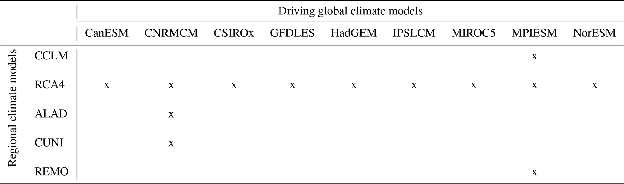
The methodological framework is presented with the sample of RCM simulations from the EURO-CORDEX initiative (Jacob et al., 2013; http://www.euro-cordex.net/, last access: 30 April 2018) together with their driving GCMs. We use 13 RCM simulations driven by nine different GCMs. All RCM simulations have 0.44^∘ horizontal resolution. The RCM simulations were conducted for the period 1951–2100, with some of them starting in 1971 or ending in 2098. We therefore concentrate on the period 1971–2098. After the year 2006 model simulations incorporated the representative concentration pathway RCP8.5 (van Vuuren et al., 2011). The GCM simulations were performed under the CMIP5 protocol (Taylor et al., 2012). The list of models is given in Table 1, and the GCM–RCM simulation matrix is given in Table 2. To identify individual simulations, we use the acronyms consisting of the abbreviations for the RCM and GCM (as defined in Table 1) connected with the underscore character. In the case of the driving GCM simulation, we use “dGCM” instead of the RCM identification.

Table 1 List of regional climate models and driving global climate models incorporated in the present study. The first column contains the acronyms used throughout the text. The type column indicates whether the model is regional (RCM) or global (GCM).

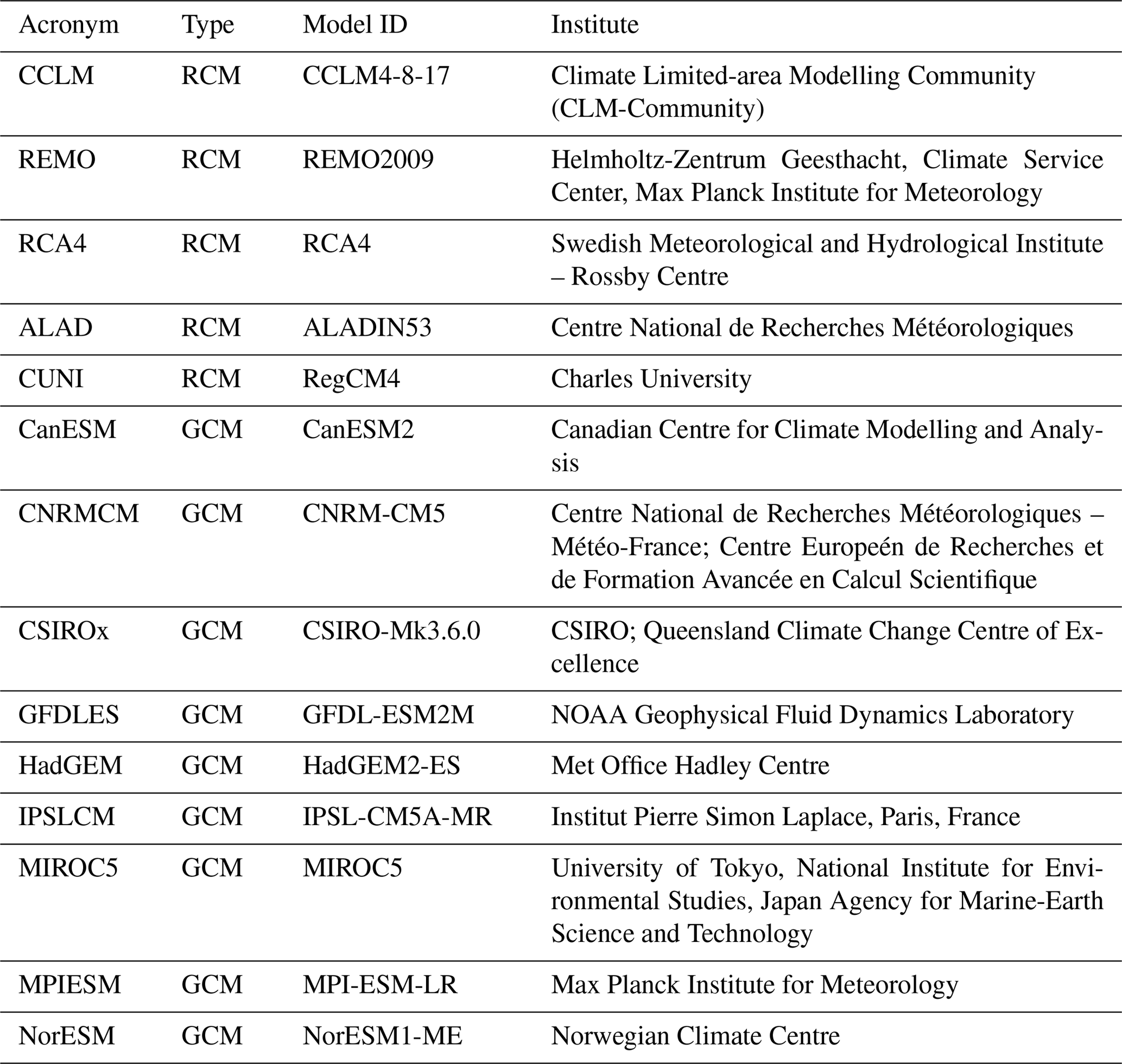
Table 2 Matrix of regional climate model simulations and their driving global climate models that are incorporated in the present study.

We concentrate on running 30-year mean changes in seasonal mean air temperature and precipitation (changes of running 30-year mean averages throughout the period 1971–2098 in comparison to the reference period 1971–2000). For the purpose of introducing the methodology, we only present two illustrative cases: winter mean air temperature changes over the British Isles (denoted as DJF tas over BI; data are shown in Fig. 1a) and summer precipitation changes over eastern Europe (JJA pr over EA; Fig. 2a).

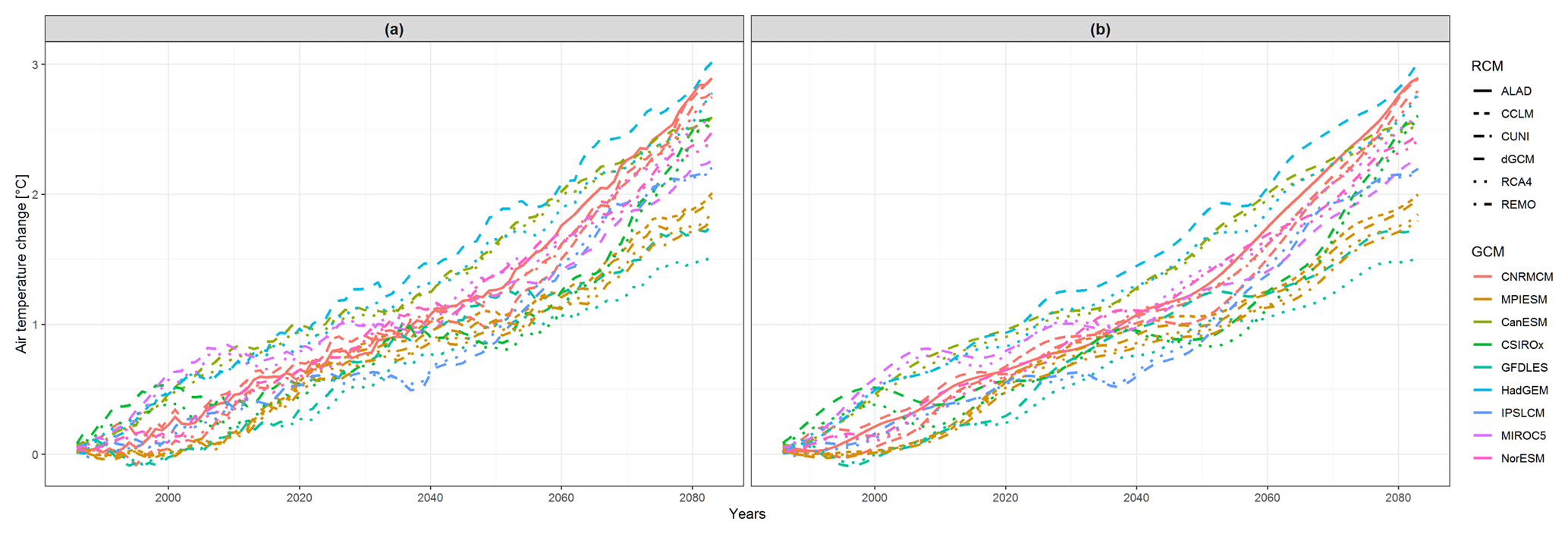
Figure 1 (a) Temporal development of running 30-year mean changes in winter (DJF) mean air temperature (changes of running 30-year mean averages throughout the period 1971–2098 in comparison to the reference period 1971–2000) averaged over the British Isles region. (b) Smoothed functional data from (a), created as described in Sect. 3. The lines in both panels are colored according to the driving global climate model (GCM), and the type of line corresponds to regional climate model (RCM). The acronyms of the model simulations are explained in Sect. 2; dGCM stands for the driving global climate model simulation.

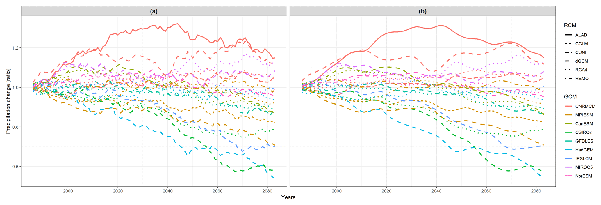
Figure 2 The same as Fig. 1, but for running 30-year mean changes in summer (JJA) mean precipitation (relative changes of running 30-year mean averages throughout the period 1971–2098 in comparison to the reference period 1971–2000), averaged over the eastern European region.

3 Methodology

3.1 Functional data analysis approach

We analyzed similarities and dissimilarities between the temporal development of simulated 30-year running mean air temperature and precipitation changes. The original dataset consisted of simulated values y_ik at central years of the 30-year periods, t_k, k=1, ..., K, ranging from 1986 to 2083 (hence K=98) for each model, i=1, ..., n. These sequences of simulations were converted to functional form using the B-spline basis system, B_j(t), j=1, ..., N. Each sequence was approximated by a spline function x_i(t) in the form

$$\begin{array}{}\text{(1)}& x_i\left(t\right)={\sum }_{j=\mathrm{1}}^N{c}_{ij}{B}_j\left(t\right),i=\mathrm{1},\mathrm{\dots },n.\end{array}$$

The B-splines B_j(t) were polynomials of order four with 20 equally spaced knots, and c_ij values were real coefficients in the B-spline basis. Such use of order-four B-splines implied N=22 basis functions. Spline functions x_i(t) were constructed in order to minimize the penalized squared error

$$\begin{array}{}\text{(2)}& {\sum }_{i=\mathrm{1}}^n{\sum }_{k=\mathrm{1}}^K{\left[y_{ij}-x_i\left(t_k\right)\right]}^{\mathrm{2}}+\mathit{\lambda }\underset{t_{\mathrm{1}}}{\overset{t_K}{\int }}{\left[{\displaystyle \frac{d^{\mathrm{2}}}{\mathrm{d}{t}^{\mathrm{2}}}}{x}_i\left(t\right)\right]}^{\mathrm{2}}\mathrm{d}t,\end{array}$$

with respect to the coefficients c_ij. The smoothing parameter λ was selected via the cross-validation method. The cross-validation method was based on the minimization of the following expression:

$$\begin{array}{}\text{(3)}& {\sum }_{i=\mathrm{1}}^n{\sum }_{k=\mathrm{1}}^K{\left[y_{ij}-x_i(t_k,\mathit{\lambda },-k)\right]}^{\mathrm{2}},\end{array}$$

where $x_i(t_k\mathit{\lambda },-k)$ denotes the leave-one-out estimator of x_i(t) omitting the k-th observation (t_k,y_ik). The actual calculation is based on minimization of the error of $x_i(t,\mathit{\lambda },-k)$ using a smoothing operator – see, for example, Craven and Wahba (1978) for details. The representative examples of the functional data from panel (a) of Figs. 1 and 2 are depicted in panel (b) of the respective figures.

One of the aims of this study was to explore the first derivative of the response function. Thus, the first derivative curves $x_i^{\prime }\left(t\right)$ were expressed in a similar manner, using the same B-spline basis with coefficients $c_{ij}^{\prime }$:

$$\begin{array}{}\text{(4)}& x_i^{\prime }\left(t\right)={\sum }_{j=\mathrm{1}}^N{c}_{ij}^{\prime }{B}_j\left(t\right),i=\mathrm{1},\mathrm{\dots },n.\end{array}$$

All subsequent analyses were conducted separately for both x_i(t) and $x_i^{\prime }\left(t\right)$.

For the representation of functional data in statistical software R (R Core Team, 2013), we used the package fda (Ramsay et al., 2017). It provides several basis options for functional data including the B-splines presented above and further functional data processing techniques.

Since the time series analyzed in the present study are relatively smooth, a metric and a semimetric were constructed to represent the distance separation between two curves (note that the smaller the cross distance, the more similar the two curves are). Such an approach seems to be appropriate, e.g., Pokora et al.(2017). Let f₁ and f₂ be two curves, specifically two cubic smoothing splines in our case. A well-known and widely-used distance between given curves f₁ and f₂ is the L₂ metric, d₀(f₁,f₂). It is a nonnegative number, whose square is defined as the integral

$$\begin{array}{}\text{(5)}& d_{\mathrm{0}}^{\mathrm{2}}\left(f_{\mathrm{1}}{f}_{\mathrm{2}}\right)=\underset{t_{\mathrm{1}}}{\overset{t_K}{\int }}{\left[f_{\mathrm{1}}\left(t\right)-f_{\mathrm{2}}\left(t\right)\right]}^{\mathrm{2}}\mathrm{d}t.\end{array}$$

Let us call this common metric d₀ distance (Euclidean distance).

Similarly, a common way to build a semimetric between two curves is to consider the L₂ distance between the first derivatives of the curves. More precisely, given two curves f₁ and f₂, we define the d₁ distance d₁(f₁,f₂) as a nonnegative number, whose square is given by the integral

$$\begin{array}{}\text{(6)}& d_{\mathrm{1}}^{\mathrm{2}}\left(f_{\mathrm{1}}{f}_{\mathrm{2}}\right)=\underset{t_{\mathrm{1}}}{\overset{t_K}{\int }}{\left[f_{\mathrm{1}}^{\prime }\left(t\right)-f_{\mathrm{2}}^{\prime }\left(t\right)\right]}^{\mathrm{2}}\mathrm{d}t.\end{array}$$

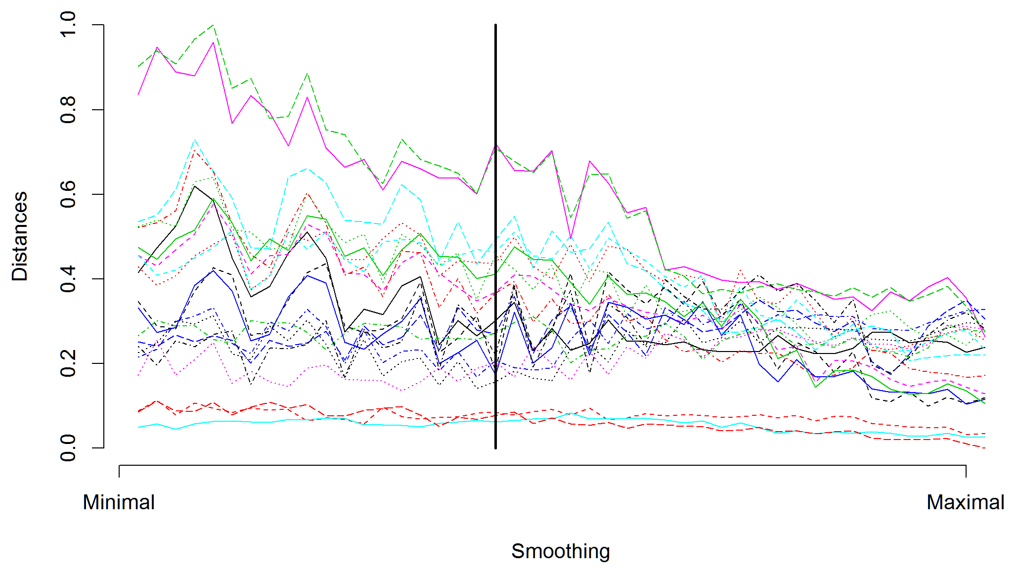
Figure 3 illustrates examples of two parts of time series that are evaluated as quite different with a large distance d₀=112.8 but are similar with a relatively small distance d₁=1.56. The main point is that the values of the semimetrics are inferred solely based on the chosen feature (e.g., Euclidean distance for d₀) and are independent of other time series characteristics. In Fig. 3 it is clearly seen that unlike d₀, the d₁ semimetric does not take into account the mutual bias of the two time series. It only focuses on the character of their temporal development. The analysis of sensitivity to the amount of smoothing was carried out. The mutual distances of the curves do not strongly depend on the smoothing parameter, as shown in Figs. 4 and 5.

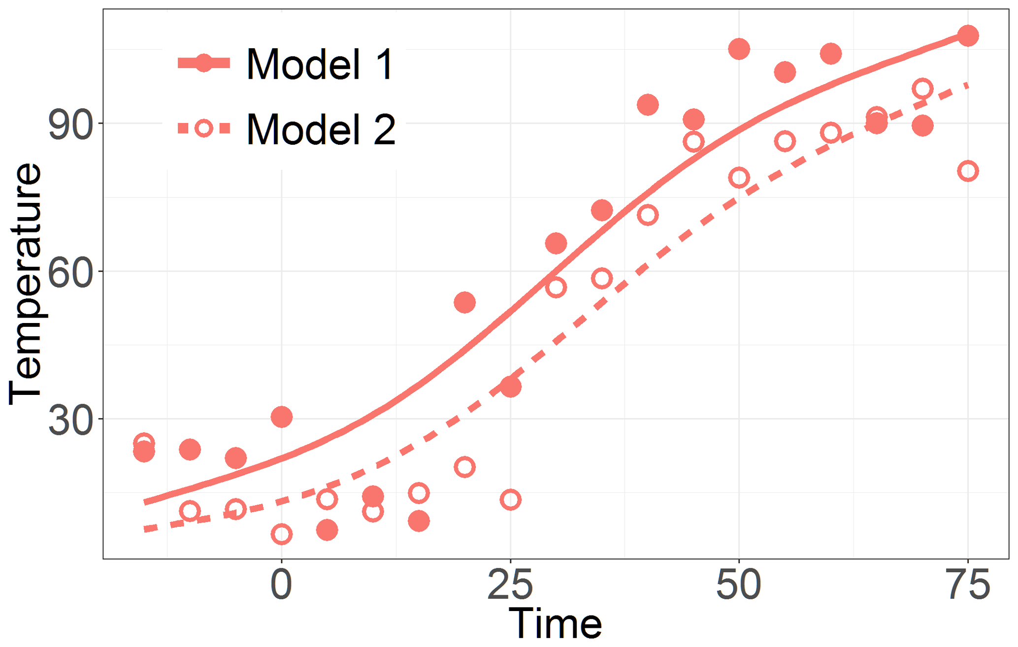
Figure 3 Illustration of the functional data analysis approach for evaluation of time series similarity. The two arbitrarily chosen time series shown here (Model 1 and 2) are evaluated to be quite different when based on d₀ but are similar when based on d₁.

Figure 4 Normalized d₀ distances between simulated air temperature curves (data are shown in Fig. 1a) of randomly selected model and other models, which depend on amount of smoothing. Starting values represent d₀ distances between original curves, and values at the end represent d₀ distances for oversmoothed data. The vertical line depicts the amount of smoothing used in the presented study.

Figure 5 The same as Fig. 4, but for distances d₁.

3.2 Visualization of the similarities

For visualization of mutual distances based on FDA semimetrics we use layout graphs created using the ForceAtlas2 algorithm (Jacomy et al., 2014) within the Gephi software (https://gephi.org/, last access: 31 May 2018). In these graphs individual members of the multi-model ensemble are visualized as nodes (each model simulation corresponding to a single node). The ForceAtlas2 algorithm creates a force-directed layout of the underlying data. The network of the nodes is created by simulating a physical system and its movement. The nodes are repulsed from each other in analogy to charged particles. At the same time the edges between the nodes attract them like springs (Jacomy et al., 2014). The iterative procedure of finding the nodes positions results in an equilibrium state which corresponds to the final network.

The interpretation of the layout graphs is straightforward. The closer the nodes are to each other, the lower the mutual distance of corresponding simulations, according to the semimetric of interest. The larger the node, the higher the number of close neighbors, meaning more similar simulations (with similarity defined by the values of selected semimetric). The edges between nearest 10 % of neighbors are made visible. The colors indicate the driving GCM.

4 Application of the methodology

Figures 1 and 2 illustrate the data used for the presented analysis. The lines are colored according to the driving GCM, and the type of line corresponds to RCM. The purpose of the presented methodology is to describe the structure of the multi-model ensemble based on mutual relationships between simulations over the whole investigated time period and evaluate whether the temporal development of the simulated changes is influenced more strongly by the driving GCM or the nested RCM. The first step is the calculation of mutual distances between the curves corresponding to individual ensemble members using the FDA semimetrics d₀ and d₁ defined in Sect. 3. In order to compare two semimetrics with substantially different ranges, we transform the values to the interval [0,1] in both cases. To facilitate viewing, we display the results in a pixel plot (see Figs. 6 and 7) with a temperature–color code (or heat map, with a redder color for more similarity and a brighter color for less similarity).

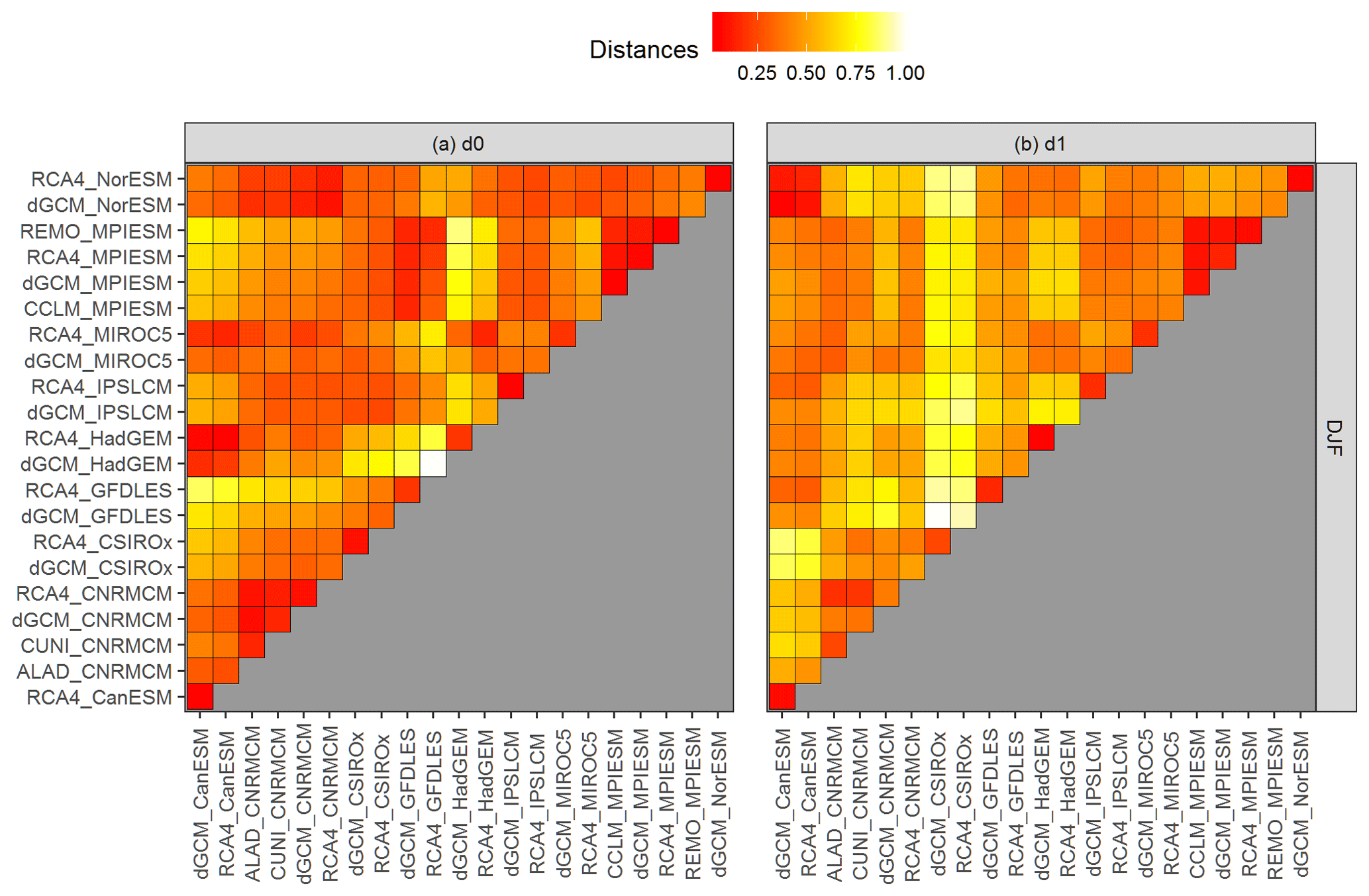
Figure 6 (a) Heat map of the d₀ distances for running 30-year mean changes in winter (DJF) mean air temperature over British Isles (the curves are shown in Fig. 1b, underlying data are shown in Fig. 1a) with redder color for more similarity and brighter color for less similarity between respective curves. The values of the semimetric d₀ are scaled to the interval [0,1]. The acronyms of the model simulations are explained in Sect. 2. The definition of the distances is explained in Sect. 3.1. (b) is the same as (a), but for d₁ distances.

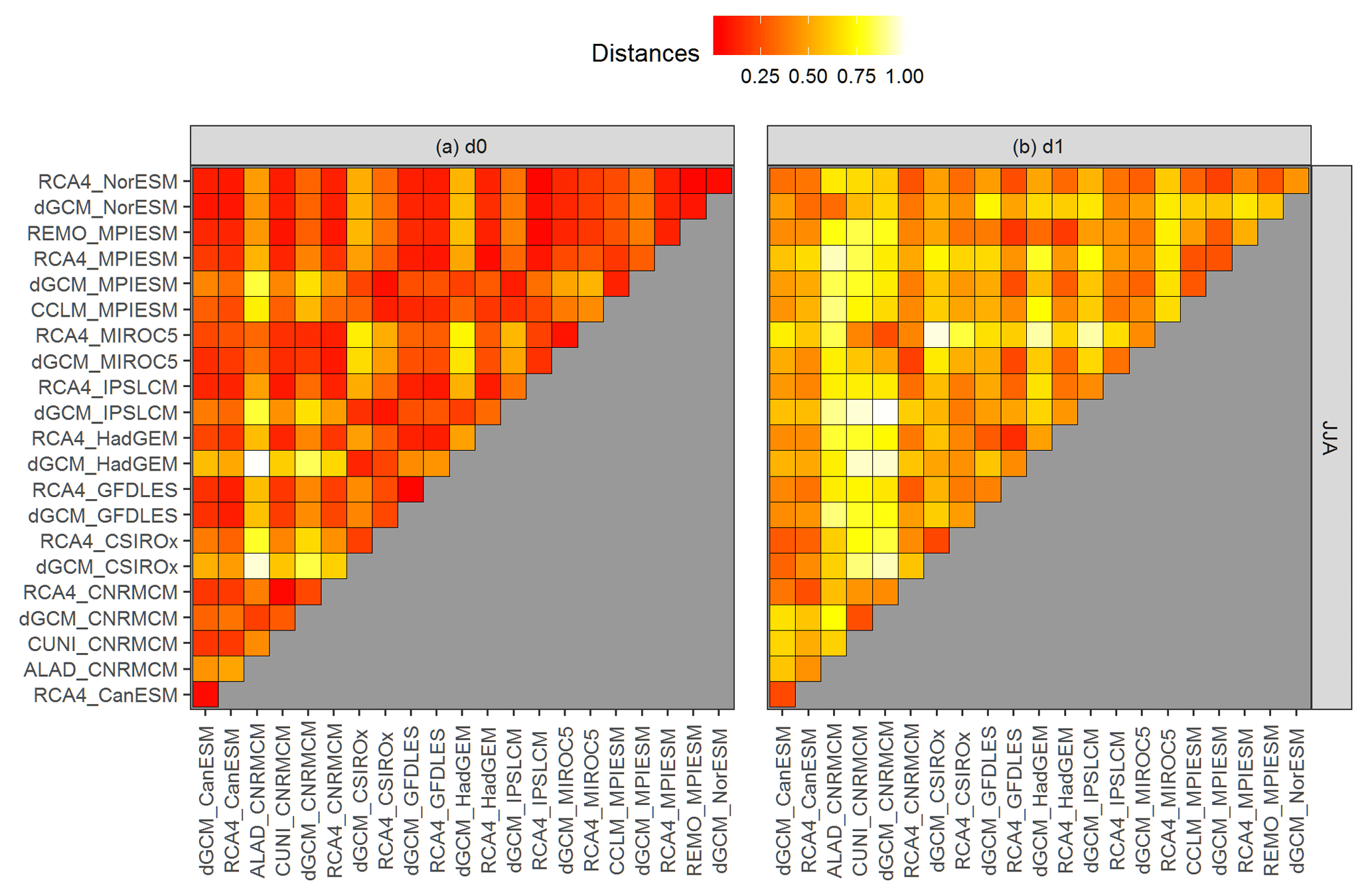
Figure 7 The same as Fig. 6, but for running 30-year mean relative changes in summer (JJA) mean precipitation over eastern European region (the curves are shown in Fig. 2b, underlying data are shown in Fig. 2a).

Figures 6 and 7 present the values of d₀ (panel a) and d₁ (panel b) distances for the two chosen datasets presented in Figs. 1 and 2. Firstly, there are clear differences between the evaluation based on d₀ and d₁ semimetrics, because each of them is based on different aspects of evaluated curves. It is well apparent from the comparison of maximum distances. In the case of JJA pr over EA (Fig. 7), the d₀ distance is the largest for the driving HadGEM GCM (dGCM_HadGEM) and ALADIN RCM driven by CNRMCM (ALAD_CNRMCM). These two simulations effectively represent lower and upper bounds of the multi-model ensemble (Fig. 2). In contrast, according to d₁ the most dissimilar time series are GCM simulations by IPSLCM and CNRMCM (Fig. 7b), because their temporal development has largely an opposite sign, even though they do lie “inside” the multi-model ensemble (Fig. 2).

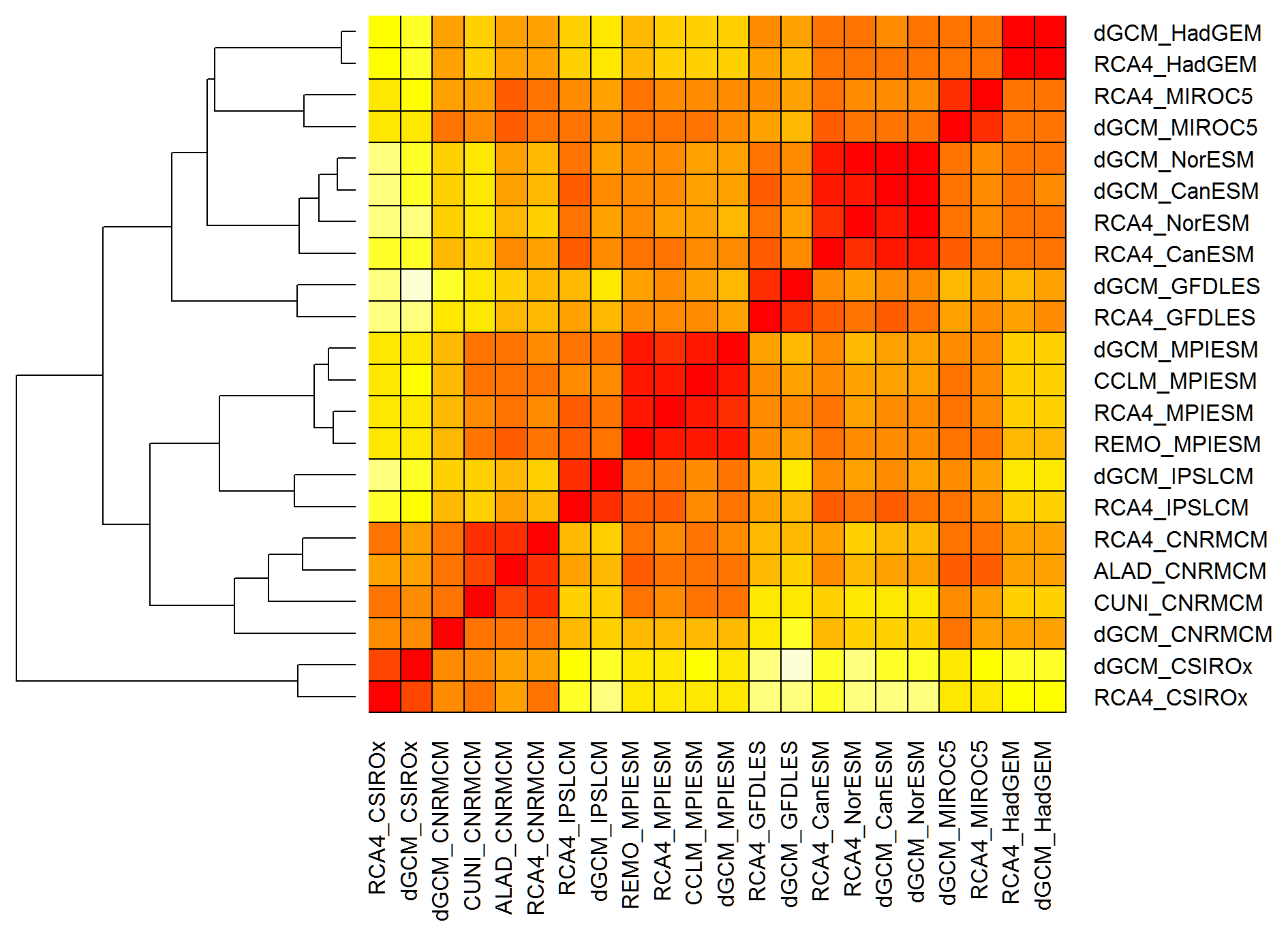
Figure 8 An example of the dendrogram resulting from hierarchical cluster analysis based on d₁ distances for running 30-year mean changes in winter (DJF) mean air temperature over British Isles (underlying similarity matrix in Fig. 6b).

The second step of the proposed methodology is to quantitatively evaluate and visualize the similarity between simulations and their clustering according to their mutual distances. This would traditionally be done by means of hierarchical cluster analysis which arranges the members of the multi-model ensemble into a dendrogram, as shown for example in Fig. 8 for the DJF tas over BI based on d₁ (R heatmap.2 function from the gplots package was used for the dendrogram creation; see Supplement). However, the interpretation of the dendrograms might not be straightforward, and relatively similar simulations might be assigned to quite remote clusters. In our example (Fig. 8) this is the case for the simulations of HadGEM and CNRM GCMs which are assigned to two remote clusters, even though their mutual d₁ distances are among the lowest in the whole ensemble (the same applies to RCM simulations driven by these two GCMs; Fig. 6b). A similar result can be seen in the case of CNRM and MIROC5 GCMs. To overcome this hurdle we propose an innovative method of visualization of the similarities based on evaluated semimetrics distances, using the layout graphs (see Sect. 3.2). Figures 9 and 10 show the layout graphs for the two investigated cases. The main advantage of the layout graphs in comparison to classical dendrograms is that the structure of the ensemble is shown in 2-D, therefore the mutual distances are seen easily. The relationships noted above between the HadGEM, MIROC5 and CNRM clusters are easily interpreted using the layout graph (Fig. 9b).

Figure 9 (a) Layout graph based on d₀ distances for running 30-year mean changes in winter (DJF) mean air temperature over the British Isles (underlying similarity matrix in Fig. 6a). (b) The same as (a), but for d₁ distances (underlying similarity matrix in Fig. 6b).

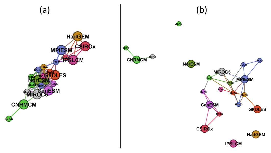
Figure 10 The same as Fig. 9, but for running 30-year mean relative changes in summer (JJA) mean precipitation over eastern European region (underlying similarity matrices in respective panels of Fig. 7).

5 Case study results

The methodology described in Sect. 3 was applied to the modeled temperature and precipitation changes from the EURO-CORDEX multi-model ensemble and the respective driving GCMs for eight large European domains (Christensen and Christensen, 2007). Here we only show two cases in order to illustrate the ability of the proposed method to assess the relationships within the members of the multi-model ensemble. These two sample cases, DJF tas over BI and JJA pr over EA, were chosen because they differ in terms of the results obtained by application of the proposed methodology, and the results are quite illustrative.

Since we analyze simulations incorporating RCP8.5, which assumes a rise in greenhouse gas concentrations during the whole 21st century, it is not surprising that all models give a rise in DJF near surface air temperature over the BI region throughout this period (Fig. 1). The RCMs tend to give a generally lower temperature change than their driving GCMs, except for RCMs driven by CNRMCM, MPIESM and MIROC5. Regarding the simulated changes in summer mean precipitation over the EA region (Fig. 2), the model simulations disagree on the sign of precipitation change, and the multi-model ensemble has quite a large variance. Some RCMs project larger changes than their driving GCMs (e.g., ALADIN driven by CNRMCM), and some give smaller changes (RCA4 driven by IPSLCM).

Based on d₀, the distances calculated for JJA pr over EA are mostly quite low (lower than 0.25) with a couple of outliers, namely ALAD_CNRMCM and driving simulations of HadGEM and CSIRO (Fig. 7a). The d₀ distances for DJF tas over BI are more evenly distributed (Fig. 6a), because there are not so many distinct outliers. The d₁ distances are higher than d₀ values in both regions and are generally higher for JJA pr over EA than for the other case (compare panel b in Figs. 6 and 7). That means that there are fewer members of the ensemble behaving in a similar manner for the EA case than for the BI case.

Regarding the influence of the driving GCM on the nested RCM simulation, based on both d₀ and d₁, for DJF tas over BI, the simulations driven by the same GCM are more clustered together than in the case of JJA pr over EA, which is visible when comparing Figs. 6 and 7 and is confirmed in Figs. 9 and 10. The clustering is stronger for d₁ results. An evaluation of Fig. 6b reveals that for DJF tas over BI the d₁ distance of the RCM simulation and its driving GCM simulation is close to zero in most cases as well as the mutual distances of RCA4 simulations driven by the same GCM (e.g., MPIESM, NorESM and CNRMCM). In the case of JJA pr over EA (Fig. 7b) the d₁ distances tend to be higher and rather independent of the driving GCM. For example, the distance between the simulations of RCA4 and REMO, both driven by MPIESM, is larger than the distances between RCA4 simulations driven by different GCMs. What we “dig” for in Figs. 6 and 7 is clearly seen at first sight in Figs. 9 and 10, respectively. The configuration of the layout graphs confirms a strong clustering according to the driving GCM in the case of DJF tas over BI and a higher degree of interaction between GCM and RCM in the case of JJA pr over EA (compare the corresponding panels in Figs. 9 and 10).

It is clearly seen that when large-scale phenomena are responsible for output, as in the case of temperature changes over the BI region, RCMs tend to be very close to the driving GCM, and different GCMs are apart from each other (Figs. 1 and 9). On the contrary, when smaller scale processes are more at play, such as in the case of JJA precipitation changes over EA, the results are more influenced by RCMs (Figs. 2 and 10). This does not automatically imply any real added value in the sense of a more realistic simulation. Rather, it points to differences in implementation of the local processes in different RCMs. In our case, different parameterization schemes employed to simulate convection, microphysical processes in clouds and surface processes including soil moisture are possible candidates.

Regarding the three RCM simulations driven by the CNRMCM GCM (RCMs denoted here as ALAD, CUNI and RCA4), it has been recently revealed that the boundary conditions for the historical period have been flawed with an inconsistency (personal communication with members of the EURO-CORDEX community). Specifically, 2-D and 3-D fields provided to the RCMs come from different members of the ensemble of CNRMCM simulations with perturbed initial conditions, therefore they are mutually out of phase. However, our results do not show any anomalous behavior in these simulations. When we calculated the distances for the curves for the first twenty 30-year periods (i.e., those with the central year before 2005, which is the end of the historical period) and for the last 20-year periods, we found out that the distance of RCM simulations driven by CNRMCM and their driving GCM is smaller for the future period than for the reference period (not shown). That is probably partly caused by above mentioned discrepancies in the boundary conditions, but the effect is rather small.

6 Discussion and conclusions

We have presented an innovative methodology for assessment of the structure of the multi-model ensemble and mutual relationships between its members. A case study evaluating the similarities within the EURO-CORDEX multi-model ensemble extended by the driving CMIP5 GCM simulations has been performed. Attention has especially been paid to the relationship between the driving GCM and nested RCM simulations in terms of temporal development of simulated temperature and precipitation changes over two European regions. Contrary to previous studies, the assessment takes into account not only simulated values for a certain time period (reference or future) but also the character of the simulated temporal development of studied variables as a whole. This is done between two time series by generalization to functional similarity. To evaluate mutual distances of the time series we used two semimetrics based on the Euclidean distances between the simulated trajectories (d₀) and on differences in their first derivatives (d₁). The similarity between an RCM and its driving GCM points to a strong forcing and rather low influence of RCM on the simulations of temporal development of the variable of interest. The d₁ distances are bias invariant, while similarity evaluated by d₀ is largely influenced by common biases of model simulations. A small d₁ mutual distance between two simulations does not automatically imply similarity in the climate change signal for a selected time period, it rather means that the shape of the temporal development is similar.

In the current study we have chosen to concentrate on temporal behavior of the time series averaged over the large European regions. We have decided to omit the spatial information, as the comparison of spatial fields from RCMs and GCMs is complicated, mainly because of large differences in spatial resolution and also because of differences in effective spatial resolution (which depends on numerical methods incorporated in the models). We have not figured out how the spatial information could be incorporated in our current setting of the methodology. Spatial fields from GCMs are much smoother than RCMs; therefore if we convert the fields into functions, the results will be very different in nature. Smoothing (regridding) the RCM fields to a GCM-like coarse resolution would result in throwing away a lot of information.

In general, the d₀ similarity indicates agreement in the bias and climate change signal, which is influenced by various feedbacks in the climate system and which might be differently pronounced in different models. The d₁ similarity points to a similar rate (speed and sign) of climate change in time that is partly modulated by internal variability of the models, which again is governed by feedbacks and nonlinearities in the climate system.

Furthermore, we presented a new way to visualize climate model similarities, based on a network spatialization algorithm. Instead of arranging the data in a one-dimensional incremental way (like in the case of hierarchical cluster analysis resulting in dendrograms), the data are ordered on a two-dimensional plane using the layout graphs, which enables an unambiguous interpretation of the results. The interpretation is only made harder by the fact that the graph can be rotated subjectively; the algorithm (see Sect. 3.2) only places each data node relatively to all other nodes, but no absolute coordinate system is defined. Even so, it is a very illustrative way of visualization of the mutual distances between the members of a multi-model ensemble. Unlike the similar approach of multidimensional scaling used in Sanderson et al. (2015), which also results in two-dimensional visualization of inter-model distances, the layout graphs do not require defining any data node as a central (reference) point of the whole ensemble.

Previously, in PRUDENCE and ENSEMBLES projects (predecessors of EURO-CORDEX), the studies of uncertainty and GCM–RCM interactions (mainly Déqué et al., 2007, 2012) relied on the analysis of variance of the multi-model ensemble. Their results were quite straightforward and clearly interpretable but suffered from additional uncertainty connected to the necessity to fill in values for missing GCM–RCM pairs using some statistical approach. The methodology proposed in the present paper overcomes this issue and uses only the outputs of dynamical models that are available. Further, as already mentioned above, the FDA similarities evaluate the whole simulated time series and are not limited to a reference or future time period.

The results of presented case study for two basic climatic variables over two European regions show that the structure of the multi-model ensemble and the GCM–RCM interactions can differ substantially in individual cases. Therefore, before the RCM outputs are used in any applied research (e.g., studies on impacts of projected future climate change), a thorough choice of RCMs to be used is necessary. The present paper offers a convenient tool for such analysis.

The methodology could be extended to include more climatic variables. Similarly, time series with different temporal aggregation (e.g., monthly or annual time series) could be used as input for the analysis. The results of multivariate evaluation of the similarities and relationships within the multi-model ensemble could be a basis for selection of representative models to be used in impact studies. Previously proposed procedures, such as in Mendlik and Gobiet (2016) or Herger et al. (2018), could be modified to use the FDA similarities introduced here.

As explained in the Introduction, the spread of multi-model ensembles is considered to be an estimate of structural model uncertainty. For analysis of the influence of internal variability on the overall uncertainty, simulations with perturbed initial conditions can be used. Unlike GCMs, for RCMs these are not generally available. In Supplement 3, a suite of figures showing FDA similarities between five simulations of the CNRM GCM with perturbed initial conditions is provided. The aim of these figures is to illustrate the range of uncertainty stemming from internal variability. We chose the CNRM GCM to maximize the number of RCMs driven by this GCM and the number of mini-ensemble members. The figures suggest that for air temperature changes, the spread of the CNRM mini-ensemble covers almost a half of the multi-model ensemble spread (Fig. S2.1 in the Supplement). In the case of precipitation, the portion of the spread is smaller (Fig. S2.2). The d₀ and d₁ distances between the members of CNRM mini-ensemble are shown in Figs. S2.3–S2.6. To enable the comparison with the distances for the multi-model ensemble, their values before normalization are provided in Figs. S2.7–S2.10. For air temperature, the maximum inter-model distances are almost twice as large as the inter-simulation distances within the CNRM mini-ensemble (compare Figs. S2.3, S2.4 and S2.7, and S2.8). In the case of precipitation, the d₀ distances between the simulations with perturbed initial conditions are very small in comparison to inter-model distances (Figs. S2.5 and S2.9). However, for d₁ distances the difference is not so staggering (Figs. S2.6 and S2.10). The fact that the range of uncertainty connected to internal variability is relatively larger (in comparison to structural uncertainty) for air temperature than for precipitation probably points to larger overall structural uncertainty in simulation of precipitation compared to air temperature, i.e., the inter-model differences in simulation of processes connected to precipitation changes are larger than in the case of air temperature changes. However, we have to keep in mind that presented results rely only on a limited number of simulations from one GCM.

The presented methodology does not take model performance explicitly into account. However, the influence of model quality on similarity is implicitly included. Worse performing models will likely be further away from good models. Furthermore, common modeling deficiencies can lead to common similarities in the validation statistics, and the metric used can account for it. A dissimilarity between the driving GCM and the nested RCM simulations can point to a situation where the GCM does not simulate a certain physical process correctly, while the RCM improves it. Moreover, the methodology can be easily modified to serve as a mean of model performance evaluation through performing the analysis for the reference period, including the observed time series. In that case, the results could be used for definition of model weights and calculation of weighted multi-model mean. For example, in Sanderson et al. (2017) the model weights are based on inter-model distance matrices, with the distances defined by the root-mean-square difference (RMSD) between the simulations. The FDA similarities between model simulations could be used instead of the RMSD. Similarly, the inter-model distances, if calculated for the whole CMIP5 GCM ensemble, could serve as a basis for the analysis of inter-model dependencies, as recently discussed, for example, in Annan and Hargreaves (2017). Finally, it can be mentioned that the presented methodology could be extended by using the functional principle component analysis (PCA). Nowadays, the functional PCA is a very popular and powerful exploratory technique. Its applications on real data indicate that it could further improve our results.