TOPMELT 1.0: a topography-based distribution function approach to snowmelt simulation for hydrological modelling at basin scale

Enhanced temperature-index distributed models for snowpack simulation, incorporating air temperature and a term for clear sky potential solar radiation, are increasingly used to simulate the spatial variability of the snow water equivalent. This paper presents a new snowpack model (termed TOPMELT) which integrates an enhanced temperature-index model into the ICHYMOD semi-distributed basin-scale hydrological model by exploiting a statistical representation of the distribution of clear sky potential solar radiation. This is obtained by discretizing the full spatial distribution of clear sky potential solar radiation into a number of radiation classes. The computation required to generate a spatially distributed water equivalent reduces to a single calculation for each radiation class. This turns into a potentially significant advantage when parameter sensitivity and uncertainty estimation procedures are carried out. The radiation index may be also averaged in time over given time periods. Thus, the model resembles a classical temperature-index model when only one radiation class for each elevation band and a temporal aggregation of 1 year is used, whereas it approximates a fully distributed model by increasing the number of the radiation classes and decreasing the temporal aggregation. TOPMELT is integrated within the semi-distributed ICHYMOD model and is applied at an hourly time step over the Aurino Basin (also known as the Ahr River) at San Giorgio (San Giorgio Aurino), a 614 km² catchment in the Upper Adige River basin (eastern Alps, Italy) to examine the sensitivity of the snowpack and runoff model results to the spatial and temporal aggregation of the radiation fluxes. It is shown that the spatial simulation of the snow water equivalent is strongly affected by the aggregation scales. However, limited degradation of the snow simulations is achieved when using 10 radiation classes and 4 weeks as spatial and temporal aggregation scales respectively. Results highlight that the effects of space–time aggregation of the solar radiation patterns on the runoff response are scale dependent. They are minimal at the scale of the whole Aurino Basin, while considerable impact is seen at a basin scale of 5 km².

1 Introduction

Seasonal snow cover is important as storage and source of meltwater for human use, irrigation and hydropower production in many regions of the world. On the other hand, snow cover and meltwater can be a cause of disastrous natural hazards, such as floods and avalanches. Additionally, snow cover is a key factor in the weather and climate system, both regionally and globally (Armstrong et al. , 2008). Owing to society's strong need for updated information on snow conditions, snow accumulation and melt, models have been developed with a wide range of features. Approaches for snowpack computation range from empirical models (e.g. simple temperature-index models) to more-sophisticated physically based energy-balance models (Zappa et al., 2003; Vionnet et al., 2012; Essery et al., 2013; Magnusson et al., 2015; Avanzi et al. , 2016). Temperature-index models require only temperature as input and are based on the assumption of a linear relationship between this variable and melt rates, whereas energy-balance models are based on the computation of all relevant energy fluxes at the snowpack surface, and thus require extrapolation of numerous meteorological and surface input variables at the local scale (Jóhannesson et al., 1995; Cazorzi and Dalla Fontana, 1996; Hock, 1999; Hock and Holmgren, 2005; Anslow et al. , 2008; Formetta et al., 2014). Advances over the simple dependence of melt on air temperature by addition of radiation terms have been suggested in the last decades (Hock, 1999; Pellicciotti et al., 2005; Carturan et al., 2012), and are termed enhanced temperature-index (ETI) models here. In contrast to simple temperature-index models, where melt varies in space only as a function of elevation (given by temperature lapse rates), ETI models include a term for clear sky potential solar radiation. This term accounts for topographic effects (e.g. aspect, slope and shading) on the spatial distribution of melt, without the need for additional meteorological variables (e.g. global radiation and cloud data). ETI models have been found to provide a better representation of the spatial and temporal variability of melt controlled by solar radiation, when compared with simple temperature-index models, as reported by a number of authors (Cazorzi and Dalla Fontana, 1996; Hock, 1999; Pellicciotti et al., 2005; Carenzo et al., 2009, among others). Some of these approaches also better cope with the physical character of the melt process and provide a promising approach to modelling the snowpack at the catchment scale with fewer input data than energy-balance models, but allow for better model parameter transferability than standard temperature-index models (Carenzo et al., 2009).

In spite of their improved accuracy compared to simpler approaches, ETI models have been so far not integrated within lumped or semi-distributed, basin-scale hydrological modelling schemes, which are still frequently used to model sparsely gauged mountainous catchments. Integration of ETI snowpack models into lumped or semi-distributed hydrological models may have the potential to increase spatial transferability of calibrated snowpack model parameters for hydrological applications over ungauged mountainous basins, as shown by Comola et al. (2015). Another important implication of the stronger physical basis of the ETI model with respect to simpler “degree day” models is that it might be more appropriate for the study of the climate-change impact on melt regimes, as shown by Pellicciotti et al. (2005). Finally, increasing the accuracy of the modelled snow water equivalent may improve the outcomes of data assimilation procedures of remotely sensed snow cover information. In a few cases, semi-distributed models incorporating a spatial discretization in classes of elevation and aspect have been applied to represent the effect of exposition on snowmelt and adjust snowpack parameters accordingly (Klok et al., 2001; Konz and Seibert, 2010; Abudu et al., 2016). In other cases, a mean value of radiation has been used over the basin area in the same elevation band, modifying accordingly the melt parameters (Li and Williams, 2008). However, these types of tessellations have no allowance for representing the actual variations of radiation distribution over space and time, which is an important feature in ETI models (Pellicciotti et al., 2005).

This work describes a novel snowpack model (termed TOPMELT herewith), which integrates the ETI snowpack method originally developed in a spatially distributed way by Cazorzi and Dalla Fontana (1996) within a semi-distributed basin-scale hydrological model. In the model developed by Cazorzi and Dalla Fontana (1996), local snowmelt is computed by using a combined melt factor which is multiplied by a radiation index and positive air temperature. With TOPMELT, pixels with a similar radiation index and air temperature are identified by subdividing basin elevation bands into a number of radiation index classes. Then, the snowpack modelling is carried out for each class of radiation index and for each elevation band. This ensures achieving significant computational efficiency, which characterizes the temperature-index models, allowing at the same time for a stronger physical basis for ETI models. This is a potentially significant advantage when several model simulation runs should be carried out, such as in Monte Carlo-based parameter sensitivity and uncertainty estimation procedures.

The model accounts for the temporal variability of the radiation index by using local mean values of the index computed over given temporal aggregation intervals, ranging from 1 to several weeks. This means that a time-averaged solar radiation distribution is used over a given temporal interval, before substituting it with a new averaged distribution. With decreasing the updating interval, the accuracy of the model is expected to increase at the expense of the computational efficiency.

As the spatial distribution of clear sky solar radiation changes with time, a radiation class computed over two different periods may sample two different portions of the elevation band. This means that a pixel belonging to a certain class at a given time will belong to a different class at another time. TOPMELT incorporates a time-integration routine, which accounts for the temporal variability of the radiation index distribution, ensuring a consistent temporal simulation of the snowpack. Thus, TOPMELT permits full implementation of the ETI snowpack method, taking into account the seasonal evolution of the spatial distribution of solar radiation. Moreover, it provides a spatially continuous mapping of simulated snow water equivalent, in spite of the computationally efficient semi-distributed representation of basin-scale snowpack modelling. Depending on the number of radiation classes which are used in the model, the snowpack model makes use of solar radiation values which are spatially averaged over different areas. Effectively, the model resembles a classical temperature-index model when only one radiation class for each elevation band is used, whereas it approximates a fully distributed model with increasing the number of the radiation classes (and correspondingly decreasing the area corresponding to each class).

This paper describes in detail the structure of TOPMELT and of the time-integration routine. The integration of TOPMELT within the ICHYMOD hydrological model is also illustrated. Finally, results are reported from the application of TOPMELT over the 614 km² Aurino Basin at San Giorgio in the Upper Adige River system (eastern Italian Alps). The case study is exploited to (i) examine the sensitivity of the snowpack and runoff model results to the temporal and spatial aggregation of the radiation fluxes, and (ii) to identify suitable spatial and temporal aggregation intervals for model simulation. The sensitivity analysis is performed on modelled snowpack in terms of snow water equivalent and on the ensuing simulated runoff, comparing the output from simulations performed at different aggregation intervals with a reference represented by the finest aggregation levels.

2 TOPMELT structure

In TOPMELT, the basin area is subdivided into elevation bands to account for air temperature variability with elevation. Then, each elevation band is subdivided into a number of radiation classes. This is carried out by dividing each elevation band into a number n_c of equally distributed radiation classes, where the ith class contains the band sub-area corresponding to the ith percentile of the incident radiation energy. Therefore, the model spatial domain is represented by n_b elevation bands and by n_c radiation classes for each elevation band. TOPMELT deals with separate snow and glacier melt: to account for the presence of a glacier area associated to an energy class, each one of the n_b×n_c model cells is characterized by the corresponding fraction of glacier area. The spatial subdivisions controls the balance between computational efficiency and model accuracy in the snowpack model.

The following sections describe the main input and modules of the model, where an hourly temporal interval is used for model computations.

2.1 Clear sky potential radiation computation and derivation of radiation distributions

For the application of TOPMELT presented in this work, clear sky shortwave solar radiation (W m⁻²) is computed at each element of the digital terrain model (DTM) by taking into account shadow and complex topography, calculating the apparent sun motion (Swift , 1976; Lee, 1978; Oke, 1992) and the intersection of radiation with topography (Dubayah et al., 1990; Ranzi and Rosso, 1991). Diffuse radiation is computed by accounting for self-shading (by slope and aspect) and occlusions produced by the visible horizon. Since the model uses radiation values averaged over a given time interval, maps of potential radiation averaged over time are also computed. The spatial distribution of time-averaged clear sky solar radiation are calculated over each elevation band, and n_c equally distributed radiation classes are identified. For each radiation class, the mean daily cumulated clear sky radiation value is computed (termed radiation index, RI, herewith; MJ m⁻²) and used in the snowmelt computation. Radiation is pre-processed and provided as model input. Therefore, the relative module is not included in TOPMELT code, but made available as a stand-alone tool (see the code availability section at the end of the paper).

2.2 Computation of precipitation amount and phase

Snow accumulation is computed starting from estimates of precipitation and air temperature, based on air temperature and precipitation data from the available weather stations. Similarly to radiation, the model permits the use of several techniques, ranging from Thiessen's polygons to multi-quadratic interpolation (Borga and Vizzaccaro, 1997) for the estimation of basin mean areal precipitation values, which are provided to the model as input data. For the analyses reported in this work, the Thiessen method was used to calculate the mean precipitation over the basin. Air temperature data are used to estimate an unique hourly vertical lapse rate for the whole basin.

To account for gauge catch deficiencies that occur during periods of snow, precipitation data are corrected with a snow correction factor (SCF). This is a multiplier of the precipitation data which is applied when station temperature is lower than a threshold temperature T_c. Finally, the basin precipitation value p_basin is obtained by applying a non-dimensional precipitation correction factor (PCF) to account for poor spatial representativeness of rain-gauge stations.

TOPMELT computes the precipitation value at the ith elevation band p_i (mm h⁻¹) by using a vertical precipitation gradient, accounting for increased precipitation over elevation. Based on results from Tuo et al. (2016), this is obtained by means of a precipitation gradient G (km⁻¹), as follows:

$$\begin{array}{}\text{(1)}& p_i=p_{\text{basin}}\cdot \left(\mathrm{1}+G\cdot {\displaystyle \frac{h_i-h_{\text{ref}}}{\mathrm{1000}}}\right),\end{array}$$

where h_i and h_ref (m a.s.l.) are the mean altitude of the ith elevation band and of the basin respectively. Equation (1) is applied in a way to modify only the distribution of precipitation across the elevation bands without altering the value of p_basin.

PCF and G parameters are generally obtained by comparing model-based snow cover simulations with satellite-based snow-cover estimates. Since the average areal precipitation p_basin is a TOPMELT input, only G is a TOPMELT parameter. Optionally, TOPMELT permits different precipitation values for each elevation band.

Temperature T_i (^∘C) is provided as input for each elevation band and time step. In this work, a mean value of air temperature T_i over the ith elevation band is obtained by using the aforementioned vertical temperature lapse rate. Estimation of the precipitation phase (solid or liquid) is therefore performed over each elevation band, according to the threshold temperature T_c.

2.3 Computation of snow and ice melt

For the generic model cell represented by the ith elevation band and the jth radiation class, snowmelt rate f_i,j(t) (mm h⁻¹) at time t is computed taking into account air temperature, clear sky radiation and albedo. During daytime hours, the snowmelt is given by the following:

$$\begin{array}{}\text{(2)}& \begin{array}{rl}{f}_{i,j}\left(t\right)=& \text{CMF}\cdot {\text{RI}}_{i,j}\left(t\right)\cdot d\cdot \left(\mathrm{1}-{\text{ALB}}_i\left(t\right)\right)\\ & \cdot max\left[\mathrm{0},\left(T_i\left(t\right)-T_{\text{b}}\right)\right],\end{array}\end{array}$$

where T_i(t) is the elevation band temperature; RI_i,j(t) (MJ m⁻²) is the cell radiation index; d (–) is the fraction of daylight hours in a day (i.e. the number of daylight hours divided by 24); CMF (mm ^∘C⁻¹ MJ⁻¹ m² h⁻¹) is the combined melt factor, accounting for both thermal and radiative effects; alb_i (t) (–) is the albedo of snow; and T_b=0 ^∘C is a threshold base temperature. Snow albedo is computed for each elevation band based on Brock et al. (2000):

$$\begin{array}{}\text{(3)}& {\text{alb}}_i\left(t\right)=\text{ALBS}-{\mathit{\beta }}_{\mathrm{2}}\cdot \left[{\log }_{\mathrm{10}}\sum _k{T}_i\left(t_k\right)\right]\end{array}$$

where ALBS (–) is the fresh snow albedo, β₂ (–) is a dimensionless parameter, and ∑_kT_i(t_k) (^∘C) is the sum of the positive hourly temperatures exceeding the threshold base temperature T_b since the last snowfall until the current time t.

During nighttime hours, snowmelt is simulated accounting only for air temperature, as follows:

$$\begin{array}{}\text{(4)}& f_{i,j}\left(t\right)=\text{NMF}\cdot max\left[\mathrm{0},\left(T_i\left(t\right)-T_{\text{b}}\right)\right],\end{array}$$

where NMF (mm h^−1 ∘C⁻¹) is the night melt factor.

For rain-on-snow conditions (Anderson , 1976), melting is computed depending on air temperature and on the energy provided by rain:

$$\begin{array}{}\text{(5)}& f_{i,j}\left(t\right)=\left[\text{RMF}+{\displaystyle \frac{p_{i,j}\left(t\right)}{\text{COST}}}\right]\cdot max\left[\mathrm{0},\left(T_i\left(t\right)-T_{\text{b}}\right)\right]\end{array}$$

where RMF (mm h^−1 ∘C⁻¹) is the rain melt factor and COST (^∘C⁻¹) is a parameter accounting for the influence of rain on snowmelt (Carturan et al., 2012). For each model cell, the snow water equivalent (we_i,j; mm) is updated by accounting for snow accumulation, rain-on-snow, melt and freezing water. Water due to snowmelt or rainfall is first retained in the snowpack as interstitial water termed liquid water liqw_i,j (mm). When liquid water exceeds a water-holding capacity of the snowpack (termed LWT), this propagates through the snowpack at a rate DYTIME (m h⁻¹), to form net water flow at the snowpack base.

When air temperature is less than the threshold base temperature, part of the liquid water refreezes and liqw_i,j is reduced and added to the snowpack through a freezing rate, termed ice (mm h⁻¹). This is computed as follows:

$$\begin{array}{}\text{(6)}& {\text{ice}}_i\left(t\right)=\text{REFRZ}\cdot min\left[\mathrm{0},\left(T_{\text{b}}-T_i\left(t\right)\right)\right],\end{array}$$

where T_b is the threshold base temperature (Eq. 2) and REFRZ (mm ^∘C⁻¹ h⁻¹) is the freezing factor. When we_i,j is less than a threshold (termed WETH), ice melt starts. This is computed similarly to snow (Eq. 2), but where the snow albedo is replaced by a constant glacial albedo, ALBG (–), as follows:

$$\begin{array}{}\text{(7)}& \begin{array}{rl}{f}_{i,j}\left(t\right)=& \text{CMF}\cdot {\text{RI}}_{i,j}\cdot d\cdot \left(\mathrm{1}-\text{ALBG}\right)\\ & \cdot max\left[\mathrm{0},\left(T_i\left(t\right)-T_{\text{b}}\right)\right]\end{array}\end{array}$$

At night and during rainfall events, glacier melt is computed by means of Eqs. (4) and (5) respectively.

All model parameters and their values are listed in Table 1, along with variable names and units. TOPMELT is majorly sensitive to the melt factor CMF, the most significant calibration parameter of the snowmelt model. It is constant both in time and space, as the variability of the melt rate is accounted for by the radiation index and by air temperature. Other important parameters are the fresh snow albedo, ALBS; the rain melt factor, RMF, which is a constant calculated from a simplified energy budget (Anderson , 1976); the precipitation gradient G, which drives the re-distribution of precipitation with the elevation; the base temperature T_b, which defines the fusion temperature of snow and ice.

Table 1 Model parameters and variables: short name, description and measuring units. Parameters are written with capital letters, variables in lowercase.

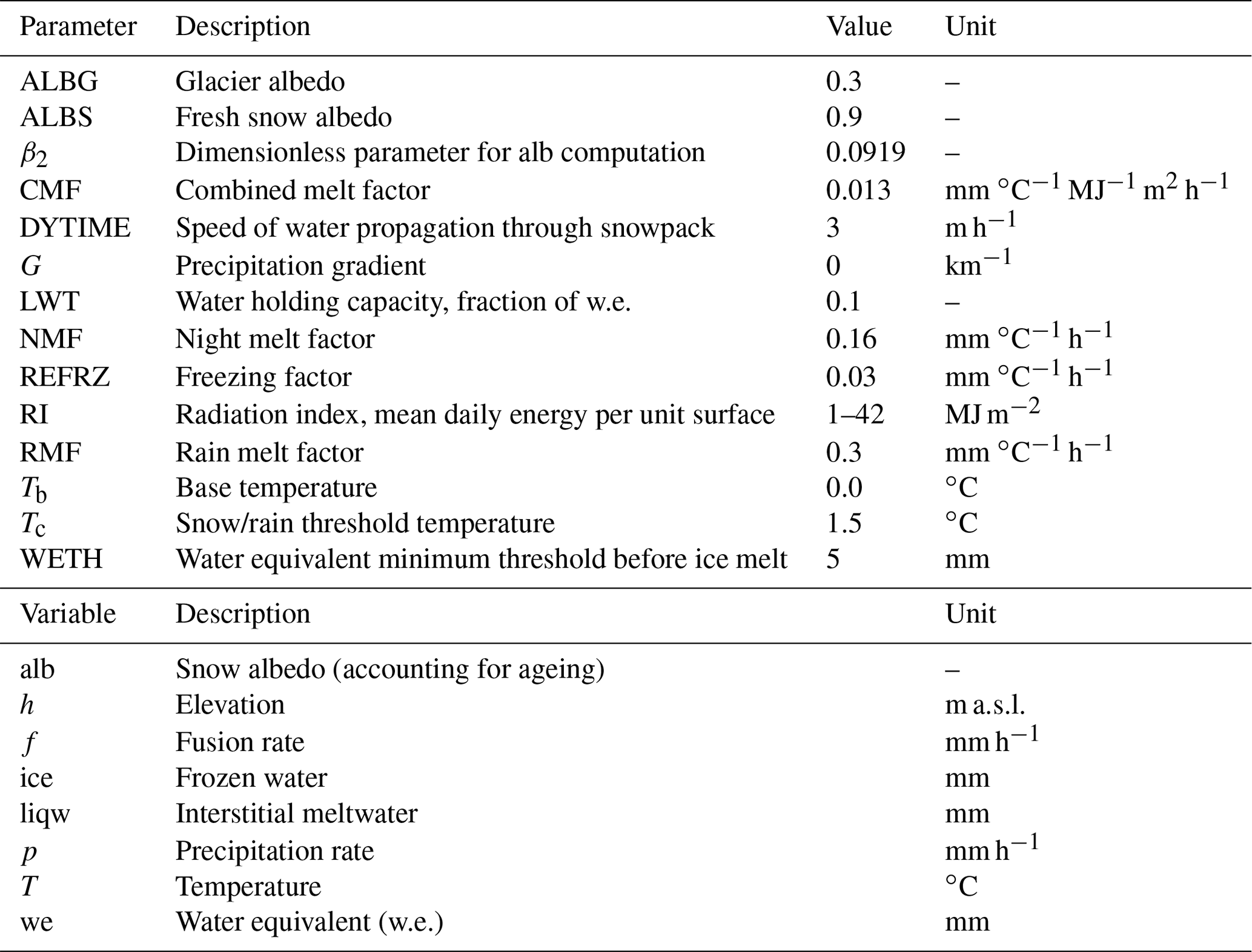
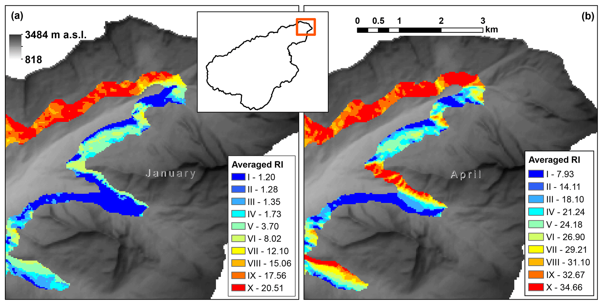
Figure 1 Comparison between radiation index distribution over the 2000–2200 m elevation band of the Aurino Basin for (a) 1 January and (b) 1 April (10 subdivision classes). The figures show the north-eastern portion of the basin and report the average radiation index M (J m⁻²), with the corresponding radiation class identified by a roman number.

2.4 Updating the radiation index distribution: the time-integration routine

As reported in the previous sections, the spatial distribution of clear sky solar radiation changes with time, based both on astronomic variation of the radiation flux and its interaction with a complex topography. This implies that the statistical distribution of the radiation index over each elevation band will be also modified and should be updated. In general a radiation class, computed at two different time steps, covers two different areas of the elevation band. Thus, a pixel belonging to a certain class at a given time will belong to a different class at another time. Figure 1 shows two different maps of RI, (representing 1 January and 1 April, from an elevation band ranging from 2000 to 2200 m a.s.l., taken from the basin selected for the case study of this work. The radiation index is distributed using 10 equally distributed classes. While the radiation index varies from 1.2 to 20.5 MJ m⁻² in January, it ranges from 7.9 to 34.7 MJ m⁻² in April. However, differences are not restricted to the magnitude of the index. Despite each class having the same area within the elevation band, their spatial distribution changes from one map to the other. Examination of the figures shows that a number of pixel belonging to class V in January are included in class IX in April.

Since the two snowpack state variables, we(t) and liqw(t), are computed at the model cell level, pixel transition from a given cell to another must be accounted for, whenever the radiation index distribution is updated with time (termed switch date here). To account for pixel transition through classes, TOPMELT implements an adjusting procedure for model state variables. The procedure is here described applied to the arbitrary cell state variable x_i,j, corresponding to the ith elevation band and the jth radiation class of the basin. When updating from one radiation index map to another, pixels from a certain class can, in principle, move to all other classes, and pixels from other classes can conversely move to that class. The x_i,j variable, which corresponds to certain model cell, should be updated accordingly. Therefore, a 2-D array accounting for the pixels' transition and the associated variables among classes is defined, namely the transition matrix M_i of the ith elevation band.

The transition matrix is n_c×n_c sized and is computed for each elevation band and is unique for each switch date of the radiation index maps. The element $M_{i,j,k}$ of the matrix represents the number of pixels moving at a switch date from the jth source class to the kth destination class, within a given elevation band i. $M_{i,j,j}$ is the diagonal element of M_i, representing the pixels that did not move from the source radiation class. Provided that the total number of pixels belonging to a class must remain constant, a property of the transition matrix is that the sum of the elements along the ith row is equal to the sum of the elements of the jth column (i.e. the number of pixels leaving a class is replaced by an equivalent number of pixels migrating from other classes):

$$\begin{array}{}\text{(8)}& \sum _{h=\mathrm{1}}^{n_{\text{c}}}{M}_{i,j,h}=\sum _{h=\mathrm{1}}^{n_{\text{c}}}{M}_{i,h,j}=N_{i,j},\end{array}$$

where N_i,j is the number of pixels in the jth radiation class within the ith elevation band. When TOPMELT switches from one radiation index map to another, the cell state variable x_i,j in the new model cell will be the sum of the pixel contribution from other classes and of the pixels remaining in the source class, where the number of incoming or remaining pixels is weighted with respect to the total number of pixels of the source class. Therefore, x_i,j is corrected through a matrix C_i of correction coefficients, relative to the ith elevation band, which can be derived from M_i through the following relation:

$$\begin{array}{}\text{(9)}& C_{i,j,k}={\displaystyle \frac{M_{i,j,k}}{N_{i,j}}}.\end{array}$$

Following Eqs. (8) and (9) that the sum of each line or column of the correction factors matrix C_i must be equal to 1,

$$\begin{array}{}\text{(10)}& \sum _{j=\mathrm{1}}^{n_{\text{c}}}{C}_{i,j,k}=\sum _{j=\mathrm{1}}^{n_{\text{c}}}{\displaystyle \frac{M_{i,j,k}}{N_{i,j}}}=\mathrm{1}.\end{array}$$

The coefficient $C_{i,j,k}$ represents the correction factor for the state variable x_i,j that must be redistributed among the other classes through the updating process, within the ith elevation band. With the updating, if x_i,j is the source class variable band and x_i,j is transformed (i.e. destination), the class variable correction is computed through the following:

$$\begin{array}{}\text{(11)}& {\widehat{\mathbf{x}}}_i={\mathbf{C}}_i\cdot {\mathbf{x}}_i,\end{array}$$

or through the equivalent forms:

$$\begin{array}{}\text{(12)}& \left[\begin{array}{c}{\widehat{x}}_{i,\mathrm{1}}\\ {\widehat{x}}_{i,\mathrm{2}}\\ \mathrm{⋮}\\ {\widehat{x}}_{i,n_{\text{c}}}\end{array}\right]=\left[\begin{array}{cccc}{C}_{i,\mathrm{1},\mathrm{1}}& C_{i,\mathrm{1},\mathrm{2}}& \mathrm{\cdots }& C_{i,\mathrm{1},n_{\text{c}}}\\ C_{i,\mathrm{2},\mathrm{1}}& C_{i,\mathrm{2},\mathrm{2}}& \mathrm{\cdots }& C_{i,\mathrm{2},n_{\text{c}}}\\ \mathrm{⋮}& \mathrm{⋮}& \mathrm{\ddots }& \mathrm{⋮}\\ C_{i,n_{\text{c}},\mathrm{1}}& C_{i,n_{\text{c}},\mathrm{2}}& \mathrm{\cdots }& C_{i,n_{\text{c}},n_{\text{c}}}\end{array}\right]\cdot \left[\begin{array}{c}{x}_{i,\mathrm{1}}\\ x_{i,\mathrm{2}}\\ \mathrm{⋮}\\ x_{i,n_{\text{c}}}\end{array}\right],\end{array}$$

and

$$\begin{array}{}\text{(13)}& {\widehat{x}}_{i,j}=\sum _{k=\mathrm{1}}^{n_{\text{c}}}{C}_{i,j,k}{x}_{i,k}.\end{array}$$

Eq. (13) represents the weighted sum of x_i,k pixels that moved from the n_c source classes to the destination kth class. Since the correction factors matrix C_i can be computed once for all simulations, the model computational efficiency is preserved.

To exemplify the computational flow and its constraints, the example of the water equivalent (w.e.) state variable is reported here. At a given radiation index switch, we_i,j, will be transferred within the ith elevation band across different classes transforming into ${\widehat{\text{we}}}_{i,j}$, for $j=\mathrm{1},n_{\text{c}}$. The total volume of snow at a given elevation band i of the destination distribution is as follows:

$$\begin{array}{}\text{(14)}& {\widehat{V}}_i^{\text{we}}=\sum _{j=\mathrm{1}}^{n_{\text{c}}}\left({\widehat{\text{we}}}_{i,j}{N}_{i,j}{A}_{\text{p}}\right),\end{array}$$

where A_p is the pixel size. Combining Eqs. (13) and (14), and provided that the number of pixels is the same for each class of the ith elevation band ($N_{i,j}=N_i$ for $j=\mathrm{1},n_{\text{c}}$),

$$\begin{array}{}\text{(15)}& \begin{array}{rl}{\widehat{V}}_i^{\text{we}}& =N_i{A}_{\text{p}}\sum _{j=\mathrm{1}}^{n_{\text{c}}}\left[\sum _{k=\mathrm{1}}^{n_{\text{c}}}\left(C_{i,j,k}{\text{we}}_{i,k}\right)\right]\\ & =N_i{A}_{\text{p}}\sum _{k=\mathrm{1}}^{n_{\text{c}}}\left({\text{we}}_{i,k}\sum _{j=\mathrm{1}}^{n_{\text{c}}}{C}_{i,j,k}\right).\end{array}\end{array}$$

Eq. (10) plus Eq. (15) yield that the transformed w.e. volume is equal to original volume:

$$\begin{array}{}\text{(16)}& {\widehat{V}}_i^{\text{we}}=N_i{A}_{\text{p}}\sum _{k=\mathrm{1}}^{n_{\text{c}}}{\text{we}}_{i,k}=V_i^{\text{we}}.\end{array}$$

Therefore, Eq. (10) is a constraint that holds conservation of w.e. through the updating process.

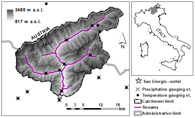
Figure 2 The Aurino River basin ending at San Giorgio with the position of the hydro-meteorological monitoring stations.

2.5 Representation of the water equivalent distribution and snow cover

The model allows one to provide the representation of spatially continuous water equivalent maps (as well as any other model cell variable) at a given time. This is carried out by exploiting a routine which links each model cell to the corresponding topographic elements, accounting for variation of the radiation index maps. Then, the water equivalent maps may be converted to snow cover maps by using suitable threshold values. In this work, we used a minimum threshold of 10 mm (Parajka and Blöschl, 2008) for the intercomparison with the MODIS snow cover products.

3 TOPMELT integration into ICHYMOD

TOPMELT is integrated within a semi-distributed hydrological model (ICHYMOD; Norbiato et al., 2008), which transforms excess precipitation plus melt contribution into runoff at the outlet of the basin. The total flow routed from TOPMELT to ICHYMOD is the areal weighted sum of each single cell flow, which is made by rainwater and excess meltwater. The model consists of a soil moisture routine and a flow routing routine.

The soil moisture routine uses a probability distribution to describe the spatial variation of water storage capacity across a basin, accordingly to the probability-distributed model (PDM) of Moore (2007). Drainage from the soil enters slow response pathways. The base discharge is routed from groundwater to the catchment outlet through a cubic law storage model. Direct runoff from the proportion of the basin where storage capacity has been exceeded is routed by means of a geomorphology-based distributed unit hydrograph (Da Ros and Borga , 1997), conceptualized by a cascade of two linear reservoirs in series. Runoff from ice melt is transferred to the outlet through two different routes, depending on glacial till imperviousness. Part of the ice meltwater is input to the soil moisture storage, while the remaining fraction flows directly to the outlet as a cascade of two linear reservoirs in series. The base discharge is routed from groundwater to the catchment outlet through a cubic law storage model. Storage-based representations of the fast and slow response pathways yield a spatially lumped representation fast and slow response at the basin outlet which, when summed, gives the total basin flow.

Losses due to evapotranspiration are calculated as a function of potential evapotranspiration and the status of the soil moisture store in the PDM. Potential evapotranspiration is estimated by using the Hargreaves method (Hargreaves and Samani, 1982).

4 TOPMELT: Impact of spatial and temporal aggregation scale

4.1 Study site, available data and model set-up

TOPMELT is applied to the Aurino River basin ending at San Giorgio, located in the Adige River system in the eastern Alps, Italy (Fig. 2).

The basin has an area of 614 km², 2.7 % of which is covered by glaciers for a total of 16.4 km². Forest covers 33.5 % of the basin, pasture and grassland 44.5 %, bare soil and rocks 21.6 % and urban areas the remaining 0.4 %. Elevation ranges from 817 to 3485 m a.s.l. Mean annual basin averaged precipitation is around 950 mm, with values ranging from 850 mm at lower elevations to 1300 mm at the highest elevations. Precipitation and temperature data at hourly time intervals are provided by 15 gauging stations (see Fig. 2 for locations), whereas observed discharge are available at the stream-gauge station in San Giorgio Aurino. The natural runoff regime is partially altered by the reservoir operations over the 25 km² Neves Basin. Basin topography is described by means of a DTM with a 30 m grid resolution.

Satellite observations of snow cover at 250 m resolution have been available for the study basin since January 2011 and are provided by an algorithm based on MODIS observations developed by Notarnicola et al. (2013a, b). With this algorithm, MODIS maps provide the presence of snow, clouds, bare soil or water bodies for each pixel or pixels with no feature detected. 50 MODIS maps are available during the period from 1 January to 30 June 2011 with a percentage of cloud cover of less than 10 %.

The basin was subdivided into 14 elevation bands of 200 m each, ranging from 800 to 3600 m a.s.l. Elevations bands were then subdivided into a number n_c of radiation classes. To assess the impact of different spatial aggregation levels of the radiation index on model results, five types of class subdivisions of the basin were considered. The elevation bands were divided into n_c=1, 5, 10, 15 and 20 classes, yielding five different spatial aggregation labelled with C1, C5, C10, C15 and C20 respectively. Similarly, to analyse the influence of using aggregation periods of the radiation index, five different updating times were used for the computation of the radiation index distribution, with durations of 1, 2, 4, 8 and 12 weeks and labelled W1, W2, W4, W8 and W12 respectively. Variable temporal and spatial discretization allows for different configurations of the space–time aggregation of the radiation index. For example, label W4-C10 refers to a model set-up with a temporal aggregation interval of 4 weeks combined with use of 10 radiation classes per elevation band. It is interesting to observe that the model set-up W12-C1 resembles a traditional temperature-index model with a radiation correction for the elevation band (as in Li and Williams, 2008), whereas the model set-up W1-C20 approximates a fully spatially distributed implementation of the enhanced temperature-index model. One should bear in mind that when just one radiation class is used, there is no need to update the distribution of the snow water equivalent.

4.2 The time-integration routine: assessment of pixel transition

An important feature of the model is the use of the time-integration routine to ensure consistency in the snowpack simulation. This routine accounts for pixel transition from one radiation index class to another at the switching time. In this section we analyse the pixel transition by using an index which represents the percentage of migrating pixels over the total number of pixels belonging to a given elevation band, as follows:

$$\begin{array}{}\text{(17)}& {\text{MI}}_i={\displaystyle \frac{{\widehat{N}}_i}{N_i}},\end{array}$$

where MI_i is the migration index of the transition, ${\widehat{N}}_i$ is the number of pixels changing class during a switch, and N_i is the number of pixels of the ith elevation band.

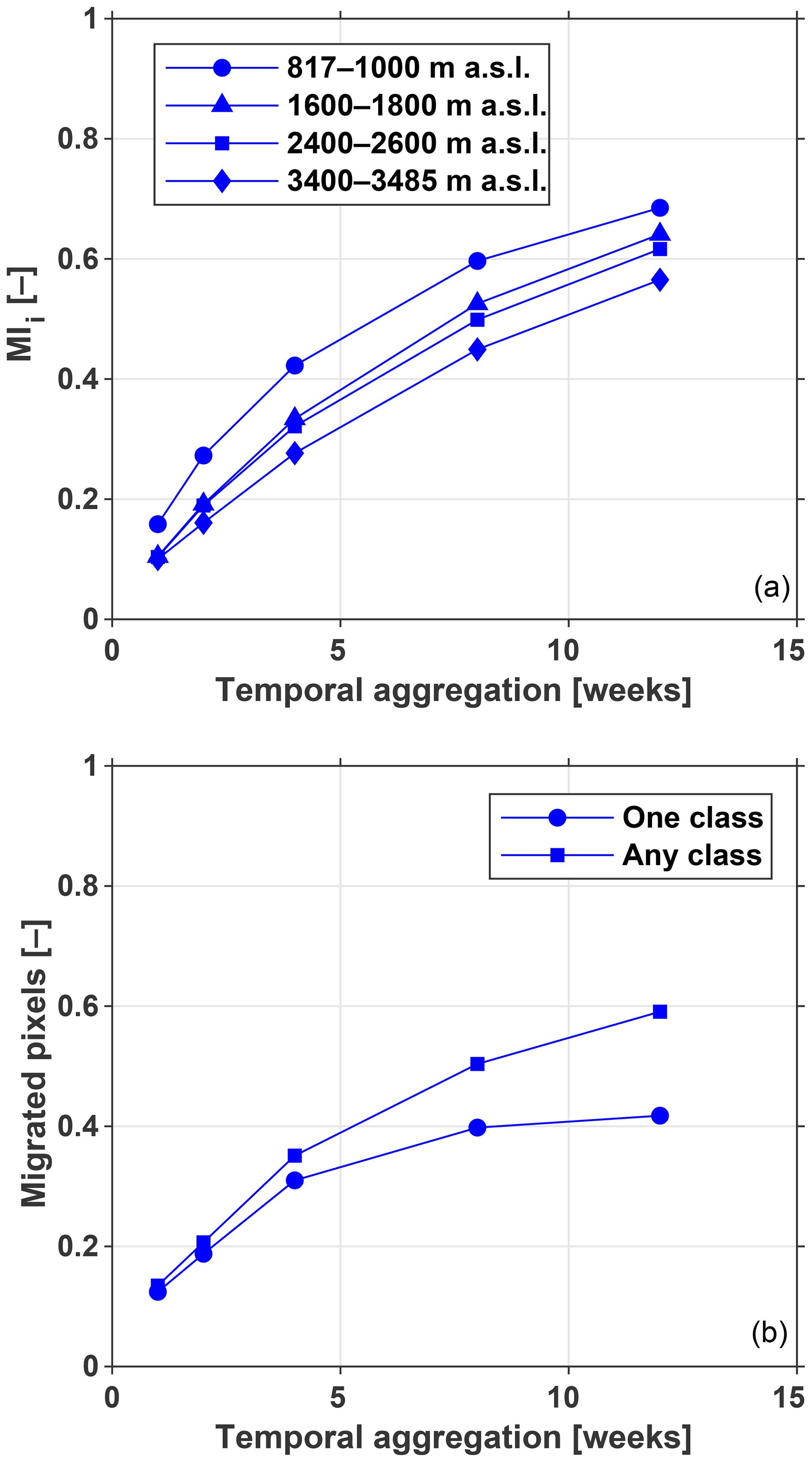
Figure 3 (a) Band migration index for the five temporal aggregations, reported for four elevation bands (lowest elevation band of 817 to 1000 m; 1600 to 1800 m; 2400 to 2600 m; and the highest elevation band of 3400 to 3485 m). (b) Fraction of migrated pixels computed for the five temporal aggregations over all elevation bands. Circles refers to pixels that migrated ±1 energy class, squares to total migrated pixels.

The percentage of migrating pixels was computed at four elevation bands: the lowest (from the lowest elevation of the basin) of 817–1000 m; two intermediate bands from 1600 to 1800 m and from 2400 to 2600 m; the highest from 3400 to 3485 m (which is the highest elevation in the basin). The analysis was performed for the five temporal aggregations by using 10 radiation index classes, reporting the mean average migration index over the various switches. Results are reported in Fig. 3a, showing that the percentage of migrating pixels ranges from up to 16 % at W1 temporal aggregation to up to 69 % at W12 temporal aggregation, with a considerable increase of the transition percentage with the increase of temporal aggregation. It is interesting to observe that the transition percentage decreases with increasing elevation of the band, i.e. with decreasing the spatial dispersion of pixels corresponding to a certain class. It is worth noting that the migration index increases with the number of radiation classes (results not shown here for brevity).

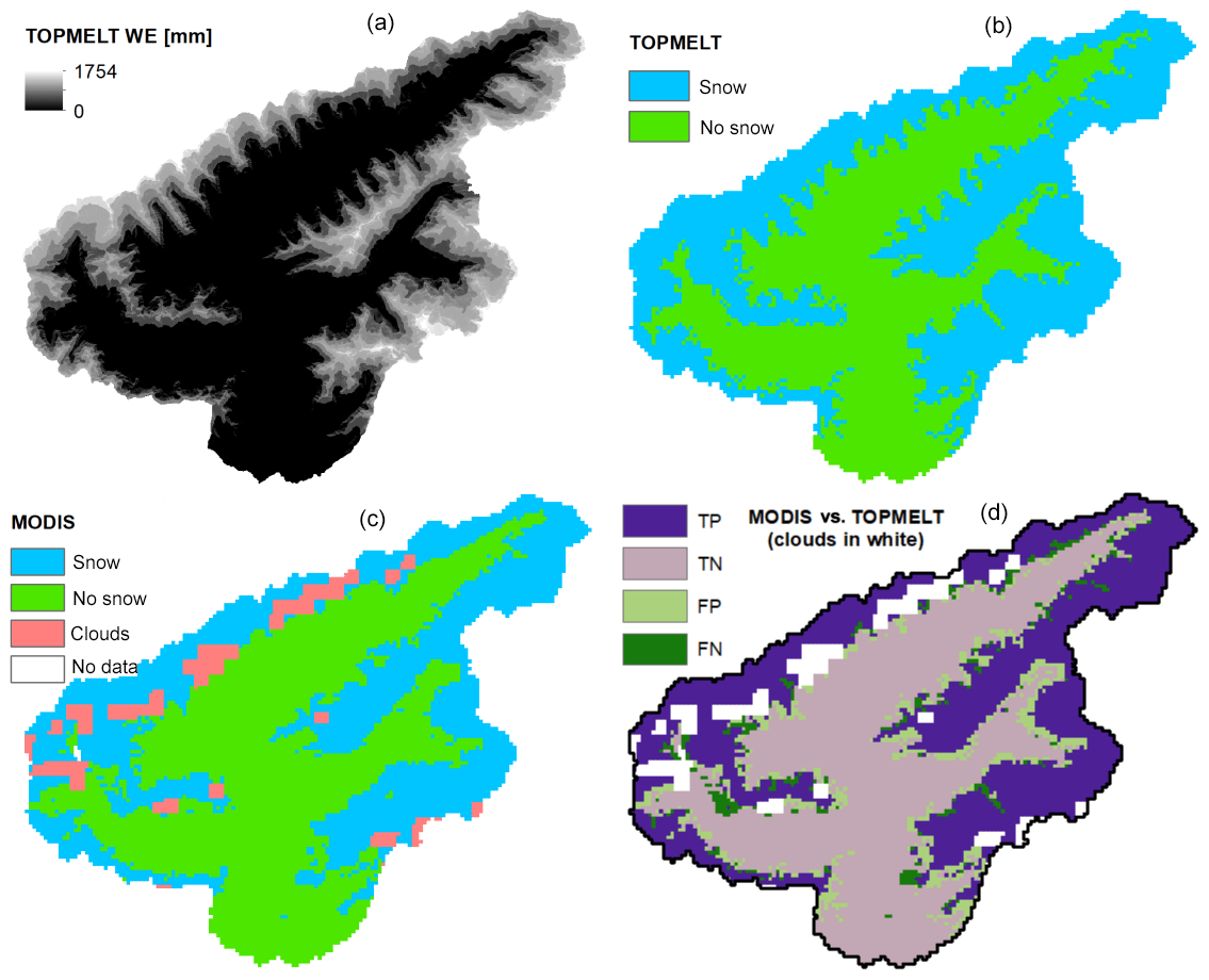
Figure 4 Comparison between simulated and MODIS-derived snow cover map. The comparison is obtained by using the model set-up W4-C10 for 6 May 2011. TP and TN are true positives and true negatives: both TOPMELT and MODIS indicate the presence or absence of snow at the pixel respectively. Similarly FP and FN are false positives and false negatives.

Finally, a specific analysis aimed to analyse the magnitude of the transition class change. To highlight this aspect, the percentage of pixels which move by only one class (for example from the second to the third radiation class) was computed and compared to the transition percentage. The percentages were computed and averaged for all the elevation bands. Figure 3b shows this comparison, by considering 10 radiation classes for the five temporal aggregations. For aggregation W12, 42 % of the pixels migrate through one class, 17 % through more than one class and only 41 % do not migrate at all. For aggregation W1, 12 % of the pixels migrate through one class, only 1 % through more than one class and 87 % of the pixels do not move from the source class at the switch time. These results agree with those reported in Fig. 3a and underline the impact of using larger temporal aggregations on the pixel transition between various classes.

4.3 Model calibration and validation

The results reported in Sect. 4.2 are obviously independent on the specification of the snowpack model parameters. However, their impact on model results (for instance, on the snow water equivalent spatial distribution) depends on the specification of model parameters.

TOPMELT and ICHYMOD parameters were identified by means of a two-stage procedure, based on comparison of the simulated outflow with the discharge measured at San Giorgio and on comparison of the simulated snow cover with MODIS data, for the period where MODIS data were available. The model set-up W4-C10 was used for the parameter identification. The following statistics were used for comparing simulated and observed discharges:

$$\begin{array}{}\text{(18)}& \text{Bias}={\displaystyle \frac{{\sum }_{t=\mathrm{1}}^N\left(Q_{\text{sim},t}-Q_{\text{obs},t}\right)}{{\sum }_{t=\mathrm{1}}^N{Q}_{\text{obs},t}}},\end{array}$$

$$\begin{array}{}\text{(19)}& \text{NSE}=\mathrm{1}-{\displaystyle \frac{{\sum }_{t=\mathrm{1}}^N{\left(Q_{\text{sim},t}-Q_{\text{obs},t}\right)}^{\mathrm{2}}}{{\sum }_{t=\mathrm{1}}^N{\left(Q_{\text{obs},t}-{\overline{Q}}_{\text{obs}}\right)}^{\mathrm{2}}}},\end{array}$$

where Q_obs,t and Q_sim,t are the observed and simulated discharge at time t, respectively, ${\overline{Q}}_{\text{obs}}$ is the average value of the observed discharges and N is the number of observations. Optimal values for bias and Nash–Sutcliffe efficiency (NSE) are 0 and 1, respectively.

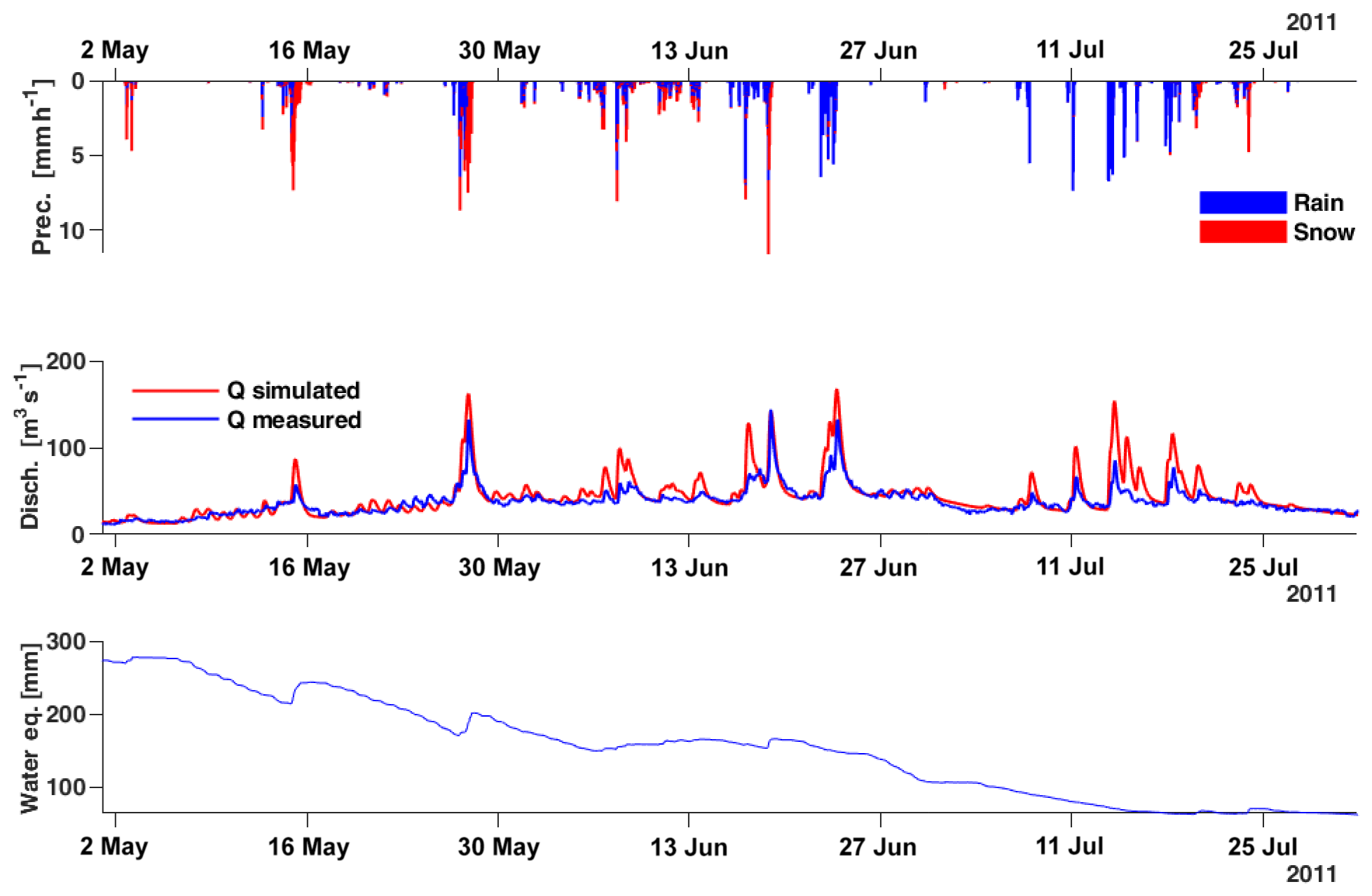
Figure 5 Comparison between simulated (W4-C10) and observed discharge at San Giorgio for the May–July 2011 period. The bottom plot displays the average w.e. over the basin.

To compare the simulated snow cover (SC) area with the MODIS observation, a snow water equivalent threshold of 10 mm was used to declare a snow-covered pixel (Parajka and Blöschl, 2008). Then, the 30 m grids contributing to one MODIS pixel were calculated, and a simulated MODIS-like pixel was considered as snow covered if the percentage of the snow-covered 30 m grid size pixels is equal to or higher than 50 %. MODIS maps with cloud coverage of less than 10 % were used for the analysis. For assessing the correspondence of simulated versus observed values, the accuracy index – ACC – skill measure, based on the contingency table, was used:

$$\begin{array}{}\text{(20)}& \text{ACC}={\displaystyle \frac{\text{TP}+\text{TN}}{\text{TP}+\text{FN}+\text{FP}+\text{TN}}},\end{array}$$

where TP are the number of true positives, i.e. where both model and observation agree on the presence of snow on the pixel; TN is the number of true negatives; FN is the number of false negatives, i.e. pixels which are snow covered according to MODIS and where the model simulates no snow; FP is the number of false positives, i.e. pixels which are free of snow according to MODIS and where the model simulates snow. ACC ranges between 0 and 1 with its optimum at 1. Application of a comparison between MODIS data and TOPMELT-simulated snow cover is exemplified in Fig. 4 for a sample date: 6 May 2011. Following Parajka and Blöschl (2008), the accuracy index (Eq. 20) was computed on a pixel base over the 50 cloud-free MODIS maps available. The resulting spatial distribution of the accuracy index is termed the overall accuracy (OA) map.

Model parameter identification was carried out by using data from 1 October 2001 to 30 September 2012 by using the model configuration W4-C10. The period from 1 October 2007 to 30 September 2012 was used for model parameter calibration, with optimization of the statistics bias, NSE and ACC, whereas model validation was carried out over the period 1 October 2001 to 30 September 2007. Model parameter optimization started from the parameterization of the ICHYMOD application by Norbiato et al. (2009). Model error statistics NSE and bias are equal to 0.71 % and 2 %, respectively, for the calibration period, and to 0.71 % and −9 %, respectively, for the validation period.

A graphical comparison of simulated (W4C10) and observed discharges is reported in Fig. 5 for the period May–July 2011, showing the general consistency of the simulation.

Figure 6 (a) Land use distribution for the catchment and (b) pixel-based overall accuracy (OA) of the comparison between simulated and MODIS-derived snow cover maps, computed from 1 January to 30 June 2011 for a total of 50 MODIS snow cover maps.

The overall accuracy map is reported in Fig. 6b, while Fig. 6b shows the land use over the catchment. The figure shows that simulated snow dynamics agrees (OA > 0.7) with MODIS snow cover detection in 71 % of the area. Lower OA corresponds to forest cover, and the north-facing slopes with forest cover are characterized by very low values of OA. This shows clearly the well-known combined effect of view geometry and forest cover on MODIS snow cover accuracy. Forests make MODIS remote sensing of snow challenging because the presence of trees complicates the monitoring of snow as trees obscure snow on the ground surface (Notarnicola et al., 2013b). View geometry may be a further major error source in MODIS snow-mapping algorithms in forested areas. This is because the gaps in forest canopies, which are essentially the detectable snow fraction in winter, are lower at off-nadir views (Notarnicola et al., 2013b).

4.4 Impact of temporal and spatial aggregation on model results

The impact of using different spatial and temporal aggregations on TOPMELT results was carried out by considering both the spatial distribution of the water equivalent and the simulated flow. In this analysis, the finest spatial and temporal discretizations, C20 and W1 respectively, were taken as a reference for the comparisons. For the water equivalent spatial distribution, the assessment was carried out for the period between 1 October 2010 and 30 June 2011, generating a distribution of w.e. at a weekly time step, for a total of 50 simulated snow maps. The intermediate subdivision into radiation classes (C10) was used for the comparison of temporal aggregations W12 to W2 with W1; Additionally, the intermediate temporal aggregation of 4 weeks (W4) was used for the comparison of spatial aggregations C1 to C15 with C20 (i.e. the reference configuration for Fig. 7a is W1-C10, for Fig. 7b is W4C20).

The NSE statistic (Eq. 19) was used to quantify the agreement between the analysis and reference w.e. distribution over space, by excluding from the comparison all the occurrences of zero water equivalence on both maps. One value of the NSE statistic was obtained for each of the 50 maps.

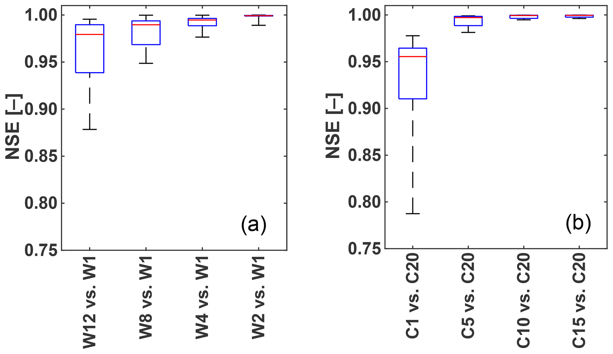
Figure 7 Box plots of NSE computed from the pixel-by-pixel comparison of the (a) temporal and (b) spatial aggregation series of w.e. maps, from October 2010 to 30 June 2011 at a weekly time step. On each box, the central mark indicates the median, and the bottom and top edges of the box indicate the 25th and 75th percentiles, respectively. The whiskers extend to the maximum and the minimum efficiency. The reference is TOPMELT with W1-C10 configuration for (a) and W4-C20 for (b).

Table 2 Nash–Sutcliffe efficiency (NSE) of the TOPMELT-ICHYMOD model at different spatial aggregation and temporal resolution, from October 2001 to October 2007.

The results are reported in Fig. 7, where the distributions of the NSE statistics are summarized by using box plots. Figure 7a summarizes the results concerning the impact of the temporal aggregation, whereas Fig. 7b shows the analysis concerning the spatial aggregation. Using the longest temporal aggregation (W12) has a noticeable impact on the results, with NSE ranging from 0.88 to 0.99. Even in this case, a considerable improvement is obtained by using a reduced temporal aggregation, such as W4. Interestingly, the results resemble the findings obtained by comparing the model set-up in terms of pixel migration. Using just one radiation class (C1) degrades markedly the accuracy of the w.e. distribution, with NSE ranging from 0.78 to 0.98. Results improve considerably by using five classes (C5).

The impact analysis on flow simulations was carried out by comparing observed and simulated flows over the validation period from 1 October 2001 to 30 September 2007. Results are reported in Table 2 by using the NSE for the various spatial and temporal aggregations. The results are at odds with those reported for the w.e. distribution, showing that the sensitivity of the modelled runoff is negligible. The reported NSE values are very close to each other, ranging from 0.70 to 0.73. The comparison of each runoff simulation to the simulations obtained by using the W4 or C10 reference models, as previously done for the snow water equivalent maps, results in NSE values always in excess of 0.99. The comparison statistics varied only in a limited way when the comparison was focused on the 1 March to 30 June period, i.e. the melting season.

These results are not unexpected. The size of the basin, which largely exceeds the correlation scale of the radiation index, together with the branching nature of the river network, provides indeed a powerful way of averaging out the heterogeneity of snowmelt processes, as shown by Comola et al. (2015), among others.

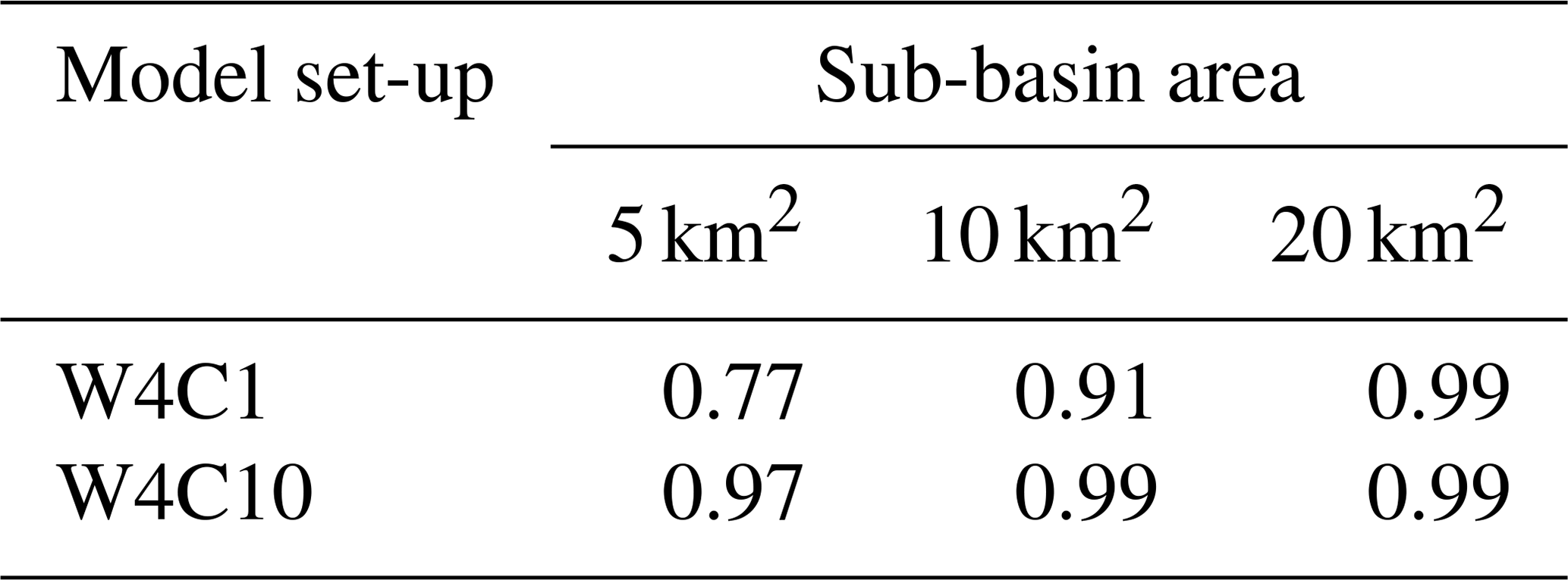
To better highlight the control exerted by the catchment size on runoff simulations, we subdivided the study basin into a number of sub-basins characterized by different drainage areas. We isolated 5 basins with mean drainage of 20 km², 10 basins with mean drainage area of 10 km² and 20 basins with mean drainage area of 5 km². The basins were identified to ensure the sampling of the whole range of solar radiation characteristics of the main basin. The model was implemented for these basins by modifying only those model parameters which depend explicitly on the area and the topography of the basin, including, of course, the distribution of the radiation index. The other model parameters were transposed from those identified for the basin ending at San Giorgio Aurino. In these comparisons, we analysed only the effect of varying the number of radiation classes. We considered only three subdivisions for the radiation classes: 1, 10 and 20 classes, and we used the runoff obtained by using the finest spatial resolution (20 classes) as a reference against which the other two were contrasted. We used a period of 4 weeks (W4) as the temporal aggregation. As a matter of fact, the simulations from the model set-up W4C1 and W4C10 were compared with the corresponding simulations from the model set-up W4C20. The NSE statistics were computed only over the 1 March to 30 June period, i.e. the melting season. The results, reported in Table 3 as an average value of the NSE statistic over the different basins, show clearly the control exerted by the catchment size on the effect of using a different number of radiation classes for runoff simulations. The differences between W4C1 and W4C20 runoff simulations are considerable (NSE = 0.77) for 5 km² area and rapidly decrease with an increase of the drainage area. At 10 km² and 20 km² NSE amounts to 0.91 and 0.99, respectively. On the other hand, no degradation is reported for runoff simulated by using 10 radiation classes instead of 20, at least for drainage areas equal to or exceeding 5 km².

Table 3 Mean value of the Nash-Sutcliffe efficiency (NSE) of the comparison between W4C1 and W4C10 TOPMELT-ICHYMOD-simulated flows and the reference flow simulations, obtained by using the W4C20 set-up, over basins of three different drainage areas: 5, 10 and 20 km². Comparisons were carried out over the 1 March to 30 June period.

5 Conclusions

This paper presents TOPMELT, a parsimonious snowpack simulation model which integrates an enhanced temperature-index model into a semi-distributed basin-scale hydrological model. This is obtained by discretizing the full spatial distribution of clear sky potential solar radiation into a number of radiation classes in each elevation band. Snowpack simulation is carried out for each radiation class, rather than for each DTM pixel. This allows one to develop synthesis in modelling approaches to snow simulation and provides the potential for analysing the impact of the spatial and temporal aggregation of radiation fluxes on model results. Furthermore, this approach reduces the computational burden, which is a key potential advantage when parameter sensitivity and uncertainty estimation procedures are carried out.

The impact of temporal and spatial aggregation of the radiation fluxes on model results is assessed by applying TOPMELT on the 614 km² Aurino River basin at San Giorgio, in the eastern Italian Alps. The analysis is carried out by examining five temporal aggregation levels (ranging from 1 to 12 weeks) and five spatial aggregation levels (obtained by subdividing each elevation band into a number of radiation classes ranging from 1 to 20), with their impact on the prediction of snow water equivalent distribution and runoff response.

The assessment of the snow water equivalent simulations clearly shows the degradation of model results when using large temporal and spatial aggregation scales, with model efficiency decreasing up to 20 %. On the other hand, the sensitivity analysis shows that averaging out the radiation index over 4 weeks and using 10 radiation classes as subdivisions has a minimal impact on model results.

Analysis of the runoff response simulations shows that the effects of the spatial patterns of snow water equivalent are strongly smoothed at the scale of Aurino Basin at San Giorgio, with minimal deviations over the different considered model set-up. Examination of TOPMELT-driven runoff results obtained over internal sub-basins ranging in area from 5 to 20 km² highlights that the effects of space–time aggregation of the solar radiation patterns on the runoff response are scale dependent, and that scale dependency is controlled by the spatial aggregation of the radiation index. Simulations obtained by using just 1 radiation class degrade in accuracy when the model is applied over basins of around 5 km², whereas runoff simulations obtained with using 10 radiation classes show very limited degradation over all basin areas considered. These results are important for driving the implementation of operational applications of TOPMELT. They may prove to be relevant for the data assimilation of remotely sensed snow cover information, which may be made more effective with increasing accuracy of modelled snow cover. They may prove to be relevant also in using the spatial transferability of enhanced temperature-index model parameters at ungauged basins.

One important implication of our results concerns the transferability of the simpler temperature-index model, which is simulated in our cases when TOPMELT is implemented by using just one radiation class. The results suggest that this spatial aggregation of the radiation patterns does not impair the spatial transferability of temperature-index models for runoff simulations of basins larger than a certain threshold, equal to 5 km² in our case study.