A comparative assessment of the uncertainties of global surface ocean CO₂ estimates using a machine-learning ensemble (CSIR-ML6 version 2019a) – have we hit the wall?

Over the last decade, advanced statistical inference and machine learning have been used to fill the gaps in sparse surface ocean CO₂ measurements (Rödenbeck et al., 2015). The estimates from these methods have been used to constrain seasonal, interannual and decadal variability in sea–air CO₂ fluxes and the drivers of these changes (Landschützer et al., 2015, 2016; Gregor et al., 2018). However, it is also becoming clear that these methods are converging towards a common bias and root mean square error (RMSE) boundary: “the wall”, which suggests that pCO₂ estimates are now limited by both data gaps and scale-sensitive observations. Here, we analyse this problem by introducing a new gap-filling method, an ensemble average of six machine-learning models (CSIR-ML6 version 2019a, Council for Scientific and Industrial Research – Machine Learning ensemble with Six members), where each model is constructed with a two-step clustering-regression approach. The ensemble average is then statistically compared to well-established methods. The ensemble average, CSIR-ML6, has an RMSE of 17.16 µatm and bias of 0.89 µatm when compared to a test dataset kept separate from training procedures. However, when validating our estimates with independent datasets, we find that our method improves only incrementally on other gap-filling methods. We investigate the differences between the methods to understand the extent of the limitations of gap-filling estimates of pCO₂. We show that disagreement between methods in the South Atlantic, southeastern Pacific and parts of the Southern Ocean is too large to interpret the interannual variability with confidence. We conclude that improvements in surface ocean pCO₂ estimates will likely be incremental with the optimisation of gap-filling methods by (1) the inclusion of additional clustering and regression variables (e.g. eddy kinetic energy), (2) increasing the sampling resolution and (3) successfully incorporating pCO₂ estimates from alternate platforms (e.g. floats, gliders) into existing machine-learning approaches.

1 Introduction

The ocean plays a crucial role in mitigating against climate change by taking up about a third of anthropogenic carbon dioxide (CO₂) emissions (Sabine et al., 2004; Khatiwala et al., 2013; McKinley et al., 2016). While the mean state in the global contemporary marine CO₂ uptake is a widely used benchmark (Le Quéré et al., 2018), underlying assumptions and limited confidence regarding the variability and long-term evolution of this sink persist. Sparse observations of surface ocean CO₂ during winter and in large inaccessible regions have been the biggest barrier in constraining the seasonal and interannual variability of global contemporary sea–air exchange (Monteiro et al., 2010; Rödenbeck et al., 2015; Bakker et al., 2016; Ritter et al., 2017). The increasing ship-based sampling effort and the ongoing development of autonomous observational platforms (e.g. biogeochemical Argo floats and Wavegliders) have improved confidence of interannual estimates of ocean CO₂ uptake in more recent years (Monteiro et al., 2015; Bakker et al., 2016; Gray et al., 2018).

The community has turned to models and data-based approaches to improve estimates of CO₂ uptake by the oceans for periods and regions with poor or no observational coverage (Wanninkhof et al., 2013b; Rödenbeck et al., 2015; Verdy and Mazloff, 2017). Ocean biogeochemical models are able to capture the general global trend in increasing oceanic CO₂ uptake shown by observations but suffer from significant regional and interannual (∼ 1 Pg C yr⁻¹) differences in their estimates because these models cannot yet accurately parameterise the marine carbonate system at computationally feasible resolutions (Wanninkhof et al., 2013b). In recent years, data-based approaches, e.g. statistical interpolations and regression methods, have become a popular alternative to biogeochemical models (Lefèvre et al., 2005; Telszewski et al., 2009; Landschützer et al., 2014; Rödenbeck et al., 2014; Jones et al., 2015; Iida et al., 2015). The regression methods try to maximise the utility of existing ship-based observations by extrapolating CO₂ using proxy variables (observable from space or interpolated). Extrapolating with proxy variables is possible due to the non-linear relationship between the partial pressure of CO₂ (pCO₂) in the surface ocean and proxies that may drive changes in surface ocean pCO₂. Improved access to quality-controlled ship-based measurements of surface ocean CO₂ through the Surface Ocean CO₂ Atlas (SOCAT) database, and satellite and reanalysis products as proxy variables have aided the development of the data-based methods (Rödenbeck et al., 2015; Bakker et al., 2016).

1.1 The current state of machine learning in ocean CO₂ estimates

With the increase in the number of statistical estimates of surface ocean CO₂, the Surface Ocean CO₂ Mapping (SOCOM) community collated 14 of these methods in an intercomparison of “gap-filling” methods (Rödenbeck et al., 2015). The intercomparison gives an overview of the SOCOM landscape, with regression and statistical interpolation approaches making up eight and four of the 14 methods, respectively (Rödenbeck et al., 2015). Two model-based approaches were also compared.

While SOCOM intercomparison did not seek to identify an optimal mapping method, it assessed members according to how well they represented interannual variability (IAV) relative to climatological surface ocean pCO₂ increasing at the rate of atmospheric CO₂ concentrations (R^iav). Two methods, the Jena-MLS (mixed-layer scheme) and MPI-SOMFFN (self-organising map feed-forward neural network), achieved lower R^iav scores compared to other members of the comparison. MPI-SOMFFN is a global implementation of a two-step clustering-regression approach and has been widely adopted in the literature (Landschützer et al., 2015, 2016, 2018; Ritter et al., 2017). The elegance of the clustering-regression approach, particularly the clustering step, is that it reduces the problem into smaller parts with more coherent variability and reduces the computational size of the problem per cluster – a beneficial attribute when using regression methods that do not scale well to big datasets.

The SOCOM intercomparison found that the gap-filling methods were in agreement in regions with a large number of seasonally resolving persistent measurements, but the different methods did not agree in regions where data were sparse (e.g. the Southern Ocean). Similarly, Ritter et al. (2017) found little agreement in the Southern Ocean on seasonal timescales, yet on decadal timescales, there was agreement on the direction of trends between gap-filling methods.

1.2 Measuring the uncertainty of estimates?

The assessment of gap-filling methods is largely limited by the distribution of the observational coverage, which is particularly true for the Southern Hemisphere where data are sparse (Rödenbeck et al., 2015; Bakker et al., 2016). The standard use of root mean squared error (RMSE) and bias as measures of uncertainty gives larger weighting to observation-heavy regions or periods compared with data-sparse regions and periods, potentially leading to underestimates of uncertainty (Lebehot et al., 2019). Note that the term “error” refers here to the error introduced by the gap-filling method relative to the observations. The R^iav score improves on the standard implementation of RMSE and bias by weighting the uncertainties annually, thus giving a less temporally biased estimate of uncertainty.

Previous studies have compared their methods' estimates to independent datasets, where measurements of pCO₂ are not included in the SOCAT datasets (Landschützer et al., 2013, 2014; Jones et al., 2015; Denvil-Sommer et al., 2019). These data serve as good validation data, particularly with the inclusion of derivations of pCO₂ from autonomous platforms in the Southern Ocean, a historically undersampled area especially during winter (Boutin and Merlivat, 2013; Gray et al., 2018).

One of the concluding statements in the SOCOM intercomparison is that pseudo or synthetic data (deterministic model output) experiments should be used to test and compare methods. Gregor et al. (2017) did just this, but their study was limited to the Southern Ocean, and the synthetic data did not fully capture the variability represented by observations, in part due to coarse synthetic data resolution (5 d mean and 1∕2^∘ spatially). The authors found that the ensemble average performed slightly better than ensemble members, in agreement with ensemble averaging approaches previously used in ocean CO₂ studies (Khatiwala et al., 2013). On the other hand, Lebehot et al. (2019) investigated the performance of an interpolation method in the North Atlantic using an ensemble of model outputs. Their approach offered a unique way of assessing a gap-filling method at places and times where no observations were made.

1.3 Aims

The main aim of this study is to present and evaluate a new machine-learning approach to estimate surface ocean pCO₂. We propose the use of an ensemble average, where we hypothesise that the “whole is greater than the sum of its parts” as the strengths of the ensemble members are often complementary in such a way to overcome the weaknesses (Khatiwala et al., 2013; Gregor et al., 2017). Further, we aim to evaluate the method for a selection of existing gap-filling methods. From this comparison, we aim not only to gain a sense of our method's performance but also the state of gap-filling based estimates; i.e. where would we be able to improve in future work?

2 Methods

There are two main components to this study: surface pCO₂ mapping with multiple methods and robust error estimation from SOCAT v5 gridded product and independent data sources. This study takes a similar two-step approach used in the Japanese Meteorological Agency – multi-linear regression (JMA-MLR) and MPI-SOMFFN approaches, where data are grouped or clustered first, and then a regression algorithm is applied separately to each group or cluster. We use the ocean CO₂ biomes by Fay and McKinley (2014) as an option for grouping. Alongside this grouping, we use an optimal K-means clustering configuration. Next, four non-linear regression methods are applied to each of the groupings. The regression methods are support vector regression (SVR), feed-forward neural network (FFN), extremely randomised trees (ERT) and gradient-boosting machine (GBM). The latter two approaches are new to the application. These methods are then compared to independent data sources. This is outlined in more detail in the experimental overview below.

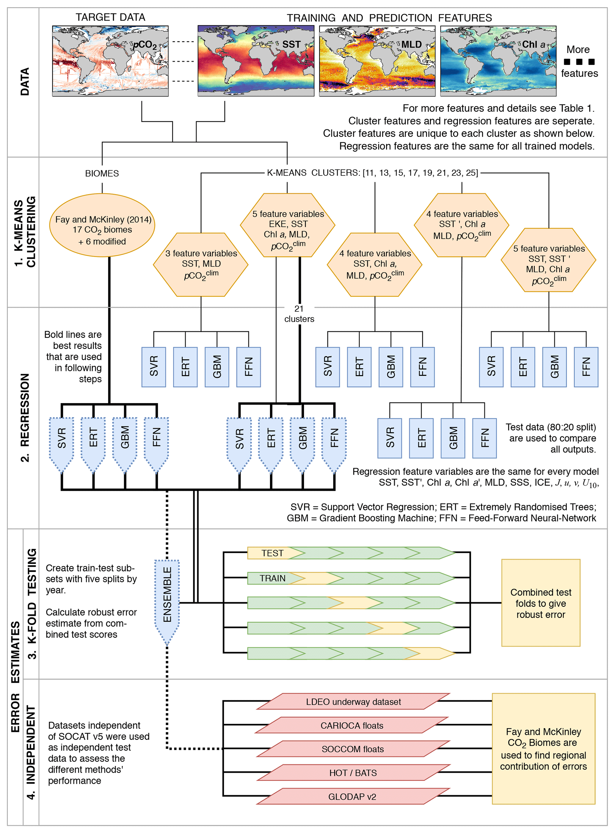
Figure 1 A flow diagram that shows the experimental procedure used in this study. Abbreviations for feature variables in the orange hexagons can be found in Table 1. All other abbreviations are given in the diagram. Details of each step are given in the text (Sect. 2.1).

2.1 Experimental overview

The experimental design, outlined below, is summarised in Fig. 1:

1. In the first step (denoted as “K-means clustering” in Fig. 1), we generate climatological biomes using the oceanic CO₂ biomes by Fay and McKinley (2014), and a selection of features variables (five combinations) and number of clusters (a range of 11 to 25 clusters, stepping by two) resulting in a total of 41 clustering configurations.

2. Four regression algorithms are applied to each clustering configuration, resulting in 164 models (described by the “regression” section in Fig. 1). The test data (isolated from the model training procedure) are used to identify the best-performing clustering configuration with annually weighted bias, RMSE and R^iav. The four regression models for CO₂ biomes and the four models from the best-performing clustering configuration (as indicated by the bold lines in Fig. 1) are used in the steps that follow. The selected eight models are averaged to create an ensemble average that is included with the eight members for further evaluation.

3. The third step (as represented by the “K-fold testing” section in Fig. 1 and Sect. 2.5) provides a robust uncertainty evaluation based on the training data (SOCAT v5). An iterative test-train approach is applied to estimate the bias, RMSE and R^iav for the complete SOCAT v5 dataset (rather than just one test split).

4. The fourth step compares the ensemble average estimates of surface ocean pCO₂ with independent test data (that are not in SOCATv5, as represented by the “independent” section in Fig. 1), which allows testing the predictive ability of the ensemble method (Sect. 2.6). Four methods from the SOCOM gap-filling intercomparison study are included for reference.

5. Lastly, all gap-filling methods are compared to identify regions where there is a divergence in the trend and seasonal cycle.

2.2 Data: clustering, training and prediction

Standard machine-learning implementation requires a training and a predictive dataset. The training dataset consists of a target variable that is being predicted (in this case, pCO₂) and one or more feature variables that have samples that correspond with target samples, e.g. sea surface temperature (SST), Chl a and mixed-layer depth (MLD) co-located in space and time, where feature variables may directly or indirectly influence the target variable. Features variables are used to predict once a machine-learning model has been trained and must thus be available for the full prediction domain.

Here, we use surface ocean pCO₂ calculated from the SOCAT v5 monthly gridded fCO₂ (fugacity of CO₂) product (hereinafter SOCAT v5, as shown in Fig. 2) as the target variable (Sabine et al., 2013; Bakker et al., 2016). SOCAT v5 is a quality-controlled dataset that contains observations of surface ocean fCO₂, which is converted to pCO₂ with

$$\begin{array}{}\text{(1)}& p{\mathrm{CO}}_{\mathrm{2}}=f{\mathrm{CO}}_{\mathrm{2}}\cdot \exp {\left(P_{\text{atm}}^{\text{surf}}\cdot {\displaystyle \frac{B+\mathrm{2}\cdot \mathit{\delta }}{R\cdot T}}\right)}^{-\mathrm{1}},\end{array}$$

where $P_{\text{atm}}^{\text{surf}}$ is the atmospheric pressure at the surface of the ocean, T is the SST in ^∘K, B and δ are virial coefficients, and R is the gas constant (Dickson et al., 2007). We used ERA-Interim $P_{\text{atm}}^{\text{surf}}$ (Dee et al., 2011) and National Oceanic and Atmospheric Administration (NOAA) daily optimally interpolated SST version 2 (dOISSTv2) that uses only Advanced Very High Resolution Radiometer (AVHRR; Reynolds et al., 2007; Banzon et al., 2016) data.

Figure 2 Map showing the distribution of the SOCAT v5 monthly gridded product (1982–2016) as a monthly climatology to show how well the seasonal cycle is represented (regardless of the year). The red shading shows grid points where the majority of data occur from May to October, and the blue shading shows grid points where the majority of data occur from November to April.

An important consideration in the use of the SOCAT database is that in situ measurements (i.e. ship measurements) are not collected at the surface. The in situ temperatures that coincide with pCO₂ in the SOCAT database are thus different from surface temperature products used to estimate pCO₂ and calculate fluxes (Goddijn-Murphy et al., 2015; Bakker et al., 2016). The discrepancy in in situ and remotely sensed temperature results in a theoretical difference between pCO₂ measured at the ship intake depth and the surface due to warming or cooling (Takahashi et al., 1993). Goddijn-Murphy et al. (2015) suggest that a correction for the theoretical difference in pCO₂ should be made using the empirical relationship between pCO₂ and temperature (Takahashi et al., 1993). While this merits further coordinated consideration by the marine CO₂ observation community, we do not apply such a temperature correction in this study, as we aim to be consistent with the earlier pCO₂ estimates from the SOCOM intercomparison (Rödenbeck et al., 2015). However, we do present the potential impact of this discrepancy in Sect. S2.4.

Table 1 Summary of the products, variables and data processing steps used for feature variables. The “usage” column indicates the features that are used for the clustering step (identified by C) and for the regression step (identified by R). Abbreviations are used in Fig. 1 and throughout the text. Basic data processing is described in the text with details in the Supplement (Sect. S1).

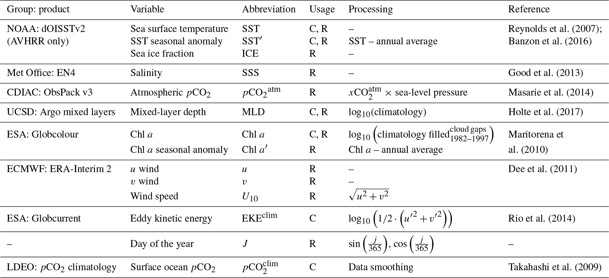
Feature variables in both the training and predictive datasets are globally gridded products, including satellite observations, in situ measurements and reanalysis products (Table 1; see Sect. S1 for details). All feature variables are gridded to a monthly frequency onto a global ${\mathrm{1}}^{\circ }\times {\mathrm{1}}^{\circ }$ resolution grid. Thereafter, data processing steps are applied as shown in Table 1 and described in detail in the Supplement (Sect. S1), with the final output being a complete dataset ranging from 1982 to 2016. Note that the clustering and regression steps use different subsets of the feature variables, as indicated in Table 1.

In this paragraph, we briefly describe the data processing steps shown in Table 1; detailed product descriptions and in-depth processing steps are in Sect. S1. We derive an additional SST feature, SST^′, by subtracting the annual mean of SST from each respective year, leaving the annual mean anomalies (Reynolds et al., 2007; Banzon et al., 2016). We use the log₁₀ transformation of the Globcolour Chl a global product (Maritorena et al., 2010). Cloud gaps and the period before the start of the product (1982–1997) are filled with the climatology (1998–2016), and high-latitude winter regions (where there is no climatology for Chl a) are filled with low-concentration random noise to be consistent with regions of low-concentration Chl a (Gregor et al., 2017). We derive an additional Chl a feature, Chl a^′, using the same procedure as described for the SST annual mean anomalies. We use a log₁₀ transformation of MLD from Argo float density profiles (Holte et al., 2017) to create a monthly climatology, thus imposing the assumption that there is no interannual variability. Wind speed is calculated from 6-hourly data using the equation in Table 1 before taking the monthly average. Atmospheric pCO₂ is calculated with $p{\mathrm{CO}}_{\mathrm{2}}=x{\mathrm{CO}}_{\mathrm{2}}^{\mathrm{atm}}\times P^{\text{atm}}$, where $x{\mathrm{CO}}_{\mathrm{2}}^{\mathrm{atm}}$ is the mole fraction of atmospheric CO₂ (from ObsPack v3 by Masarie et al., 2014) and P^atm is the reanalysed mean sea-level pressure (from ERA-interim 2; Dee et al., 2011) – further details for the procedure are in Sect. S1. The climatology of eddy kinetic energy (EKE^clim) is calculated from u and v surface current components (integrated for depth < 15 m) from the Globcurrent product (Rio et al., 2014), where u^′ is calculated as $\underset{\mathrm{¯}}{u}-u$ and similarly with v (Table 1).

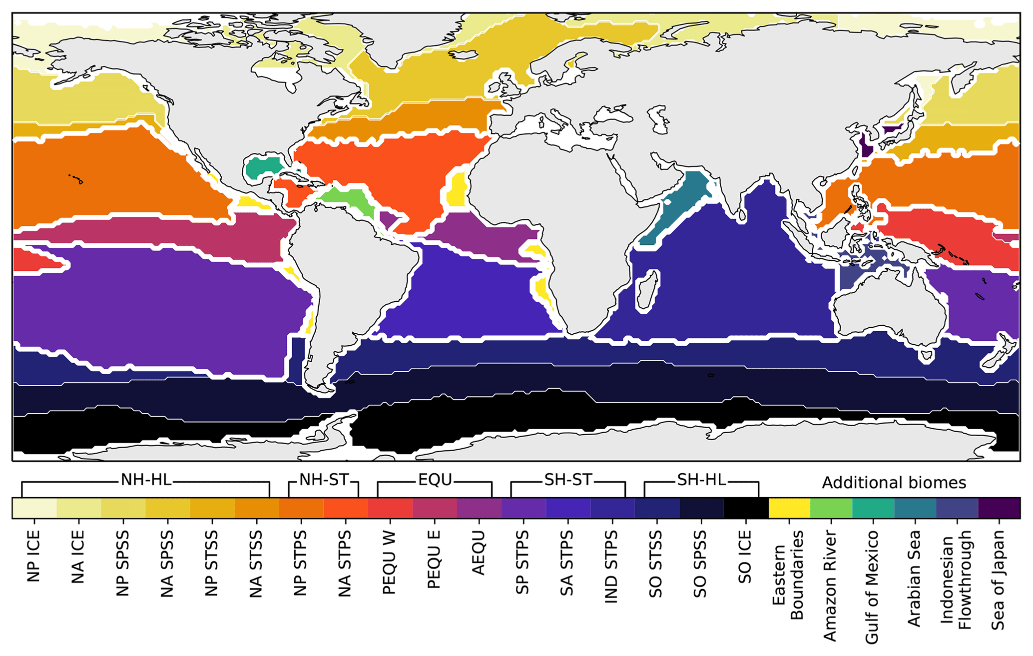
Figure 3 Regions or biomes as defined by Fay and McKinley (2014). Unclassified regions from the original data have been assigned manually in this study and are shown by the separate colours. This modified configuration of the CO₂ biomes is referred to as BIO23 in this study. The sea mask used in Landschützer et al. (2014) has been applied. For the biome abbreviations (below the colour bar), see Fay and McKinley (2014). The abbreviations above the colour bar are used in this study, where selected biomes are grouped together. Thick white lines show the boundaries of the grouped regions. Prefixes are as follows: NH is Northern Hemisphere and SH is Southern Hemisphere. Suffixes are as follows: HL is high latitudes, ST is subtropics, and EQU is equatorial.

2.3 Clustering and biomes

The seasonal and interannual variability of global surface ocean pCO₂ is complex due to interactions of various driver variables acting on the surface ocean at different space scales and timescales (Lenton et al., 2012; Landschützer et al., 2015; Gregor et al., 2018). Machine-learning algorithms applied globally struggle to represent the pCO₂ accurately unless spatial coordinates are included as feature variables (Gregor et al., 2017). This is due to the fact that pCO₂ may respond inconsistently to observable feature variables in different regions as it is not possible to observe all feature variables that drive pCO₂. A common practice to avoid the inclusion of coordinates is to separate the ocean into regions where processes that drive pCO₂ are coherent and then apply individual regressions to each region – five of the eight regression methods in Rödenbeck et al. (2015) apply this approach. We adopt two such approaches to develop regions of internal coherence with respect to CO₂ variability, namely regions defined by biogeochemical properties and clusters defined by a clustering algorithm.

Our first “clustering” approach uses the oceanic CO₂ biomes by Fay and McKinley (2014) that divide the ocean into 17 biomes. Fay and McKinley (2014) define their biomes by establishing thresholds for SST, Chl a, sea-ice extent and maximum MLD. Unclassified regions from the original biomes are manually assigned based on their geographical extent, resulting in six additional regions (Fig. 3). We maintain these as separate regions from the original Fay and McKinley (2014) biomes. Their study originally did not classify these regions in the core biomes because the physical and biogeochemical properties were not accounted for by the set thresholds from their study. This would suggest that drivers of CO₂ in these regions could be quite different from the adjacent open-ocean biomes. Note that we may refer to the modified Fay and McKinley (2014) ocean CO₂ biomes as “CO₂ biomes” or as “BIO23” from here on (Fig. 3). For later analyses, we group certain biomes together, as shown by the brackets above the colour bar in Fig. 3.

We also use K-means clustering, which groups data based on Euclidean distances. More specifically, we implement mini-batch K means from Python's Scikit-learn package (Sculley, 2010; Pedregosa et al., 2011), which is described in the Supplement (Sect. S2.2; Fig. S2). We apply clustering with various feature combinations and the number of clusters (shown by orange hexagons in Fig. 1). We tested a range of 11 to 25 clusters (stepping by two). The performance of each clustering configuration is not tested with a clustering metric; instead, we test the performance based on the test scores of the regressions in the next step as a more complete indicator of performance. We find optimal results with respect to RMSE and biases with 21 and 23 clusters. We selected 21 clusters (Fig. S2). Each method of defining regional coherence with respect to pCO₂ variability has its methodological weaknesses so in this study, we adopted the approach of incorporating both K means and CO₂ biomes into the ensemble average (Fig. 1). Although this likely weakens the geophysical meaning of the ensemble domains, we show that it strengthens the overall performance of the ensemble average.

2.4 Regression

Here, we describe the underlying machine-learning principles of regression. The co-located data (i.e. SOCAT v5) are split into training and test subsets with a roughly 80 : 20 split. The test subset is isolated from the training process to attain a reliable estimate of uncertainty. We make the split between training and test subsets based on a random subset of years in the time series (1982–2016): 1984, 1990, 1995, 2000, 2005, 2010 and 2014. We avoid using a shuffled train-test split (completely random), as this leads to artificially low uncertainties in machine-learning algorithms that are prone to overfitting (see the experiment in Sect. S2.1), where the models can reproduce the shuffled test data better, as these data are adjacent to samples of the same ship track.

We further reduce the possibility of overfitting by tuning the hyperparameters for each model to be more generalised, i.e. able to fit the data that the model has not been exposed to. The search for the optimal hyperparameters is achieved with grid-search cross validation, where a portion of the training subset is iteratively kept separate from the training process for a certain set of hyperparameters (Hastie et al., 2009). The hyperparameters that result in the best score from the grid search are used for the fit with the full training subset (see Sect. S2.3 for more details). We use a variation of K-fold cross validation called “group K fold” in Scikit-learn (Pedregosa et al., 2011). Rather than having arbitrary splits for each fold, a given grouping variable is used to split the data – in this case, years. Using years as the grouping variable reduces bias towards the second half of the time series where data are less sparse.

The train-test split and cross validation are applied identically to each of the four machine-learning algorithms for each clustering configuration. We use the following machine-learning algorithms: ERT – Geurts et al. (2006); GBM – Friedman (2001); SVR – Drucker et al. (1997); and FFNs. The details of these methods and how they were tuned are explained in the Supplement (Sect. S2.3). The first two methods, ERT and GBM, are new to this application. SVR has been implemented as a single global domain by Zeng et al. (2017), and FFN is used by several different methods, some of which are in the SOCOM intercomparison (Landschützer et al., 2014; Zeng et al., 2014; Sasse et al., 2013).

Regression performance is tested using RMSE primarily but also bias (Eqs. 3 and 4 below) and R^iav (Eq. 5), with only the models from the best averaged clustering configuration used for the rest of the study.

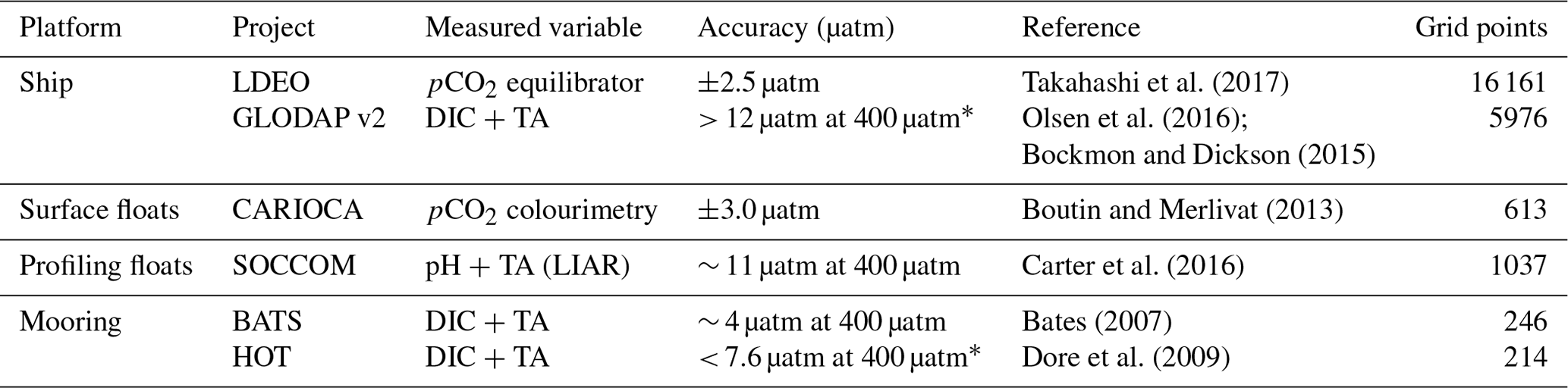
Table 2 Details for the validation datasets. The measured variables are shown (DIC is dissolved inorganic carbon; TA is total alkalinity) along with the estimated accuracy of pCO₂. This includes the propagated uncertainty in the conversion from DIC and TA to pCO₂ as defined by Lueker et al. (2000), where the estimates marked with ^* are an extrapolation of the estimates, as the DIC and TA uncertainties do not match or exceed those listed in the publication. Note that the error estimates for GLODAP v2 are larger than those shown in the table, as measurement uncertainty is defined as ±10 µmol kg⁻¹ in Bockmon and Dickson (2015). Grid points show the number of data at the same resolution as the feature variables.

2.5 Robust biases and root mean square errors

Standard practice in machine learning is to set aside a test subset of the data, as described in Sect. 2.4. We use this standard approach in the second step of our experiment (regression comparison) as an estimate of the performance for each of the machine-learning models (164 in total). However, this grouped train-test split gives a bias and RMSE estimate limited to the random test years of test subset (see Sect. 2.4). To overcome this limitation, we iteratively apply the train-test split method with multiple selections of years. The splits in the test fold are based on a subset of years spaced 5 years apart. We then refactor the five test-fold estimates into a complete test estimate (with the same structure as the original SOCAT v5), thus giving a complete estimate of bias and RMSE (Fig. 1, step 3). This robust test-estimate method ensures that correct biases and RMSE scores are reported even if methods are prone to overfitting (see Sect. S2.1 and Fig. S1). We limit this procedure to only the CO₂ biome and best clustered regressions as it has 5 times the computational cost of a single train-test split.

Figure 4 The distribution of the validation data. Details of these datasets are given in Table 2. The Hawaii ocean time series (HOT) and the Bermuda Atlantic time series (BATS) are marked as diamonds to distinguish them as time series stations.

2.6 Method validation data

For method validation, we use observation data that are not used in SOCAT (Fig. 4 and Table 2) as they are either (1) included in the Lamont–Doherty Earth Observatory (LDEO) database but not in SOCAT; (2) not measured with an infrared analyser; or (3) derived from two other variables in the marine carbonate system, where these include dissolved inorganic carbon (DIC), pH and total alkalinity (TA) – where the Southern Ocean Carbon and Climate Observation and Modeling (SOCCOM) floats use empirically calculated TA.

The uncertainty of pCO₂ that is calculated from DIC and TA is dependent on the accuracy of these two measurements, as well as the derivation of pCO₂ with dissociation constants, for which we use the CBSys package in Python (Hain et al., 2015). CBSys implements the constants from Lueker et al. (2000) that reports an uncertainty of 1.9 % standard deviation of the calculated pCO₂ where DIC and TA uncertainties are 2.0 and 4.0 µmol kg⁻¹, respectively. The measurements in GLODAP v2 are slightly larger than this at 4 and 6 µmol kg⁻¹, which would result in an error larger than 1.9 % – this is 12 µatm for a 400 µatm estimate at a hypothetical 3 % error. However, this error may be larger, as reported in Table 2, where Bockmon and Dickson (2015) showed that the uncertainty for DIC and TA is likely closer to ±10 µmol kg⁻¹. While this potentially large error range may seem concerning, we argue that the inclusion of these data in data-sparse regions is more valuable than their omission. Additionally, GLODAP v2 data have been adjusted on a per-profile basis to minimise the biases through the comparison of deep slow-changing ocean properties (Olsen et al., 2016). Williams et al. (2017) estimated the error for pCO₂ calculated empirically to be 2.7 %, where TA was calculated empirically with the locally interpolated alkalinity regression (LIAR) algorithm (Carter et al., 2016). Note that the datasets in Table 2 likely suffer from biases unaccounted for due to temperature mismatches as discussed in Sect. 2.2 (Goddijn-Murphy et al., 2015). It is important to note that each of the validation datasets are compared independently of each other, thus avoiding the complications of accounting for the biases between datasets. All pCO₂ data are then gridded to the same time and space resolution as the feature variables (monthly × 1^∘) using xarray and pandas packages in Python (McKinney, 2010; Hoyer and Hamman, 2017).

2.7 Sea–air CO₂ flux calculation

Bulk sea–air CO₂ flux (FCO₂) is calculated with

$$\begin{array}{}\text{(2)}& F{\text{CO}}_{\mathrm{2}}=k_{\text{w}}\cdot K_{\mathrm{0}}\cdot \left(p{\mathrm{CO}}_{\mathrm{2}}^{\mathrm{sea}}-p{\mathrm{CO}}_{\mathrm{2}}^{\mathrm{atm}}\right),\end{array}$$

where K₀ is the solubility of CO₂ in seawater (Weiss, 1974) and k_w is the gas-transfer velocity calculated from wind speed using formulation by Nightingale et al. (2000), as this parameterisation was the closest match to in situ observations of CO₂ fluxes (Goddijn-Murphy et al., 2016). The ERA-interim v2 wind product is used to calculate k_w. $p{\mathrm{CO}}_{\mathrm{2}}^{\mathrm{sea}}$ is from the gap-filling methods, and $p{\mathrm{CO}}_{\mathrm{2}}^{\mathrm{atm}}$ is atmospheric pCO₂. All ancillary variables required in these calculations are the same as those listed in Table 1, except for $p{\mathrm{CO}}_{\mathrm{2}}^{\mathrm{atm}}$, which is the CarboScope atmospheric pCO₂ product from Rödenbeck et al. (2014). One of the problems with the bulk estimates of sea–air CO₂ fluxes is that models of gas exchange in the surface layer of the water column are simplified, but there are approaches, such as the rapid equilibrium model, that account for more complex temperature gradients in the upper layer of the surface ocean (Wanninkhof et al., 2009; Woolf et al., 2016). However, for the sake of consistency with past studies, we use the bulk approximation of sea–air fluxes (Eq. 2), where k_w is scaled to 16 cm h⁻¹ as in the SOCOM intercomparison (Rödenbeck et al., 2015).

2.8 Relative interannual variability and interquartile range metrics

2.8.1 Regression metrics

We use bias and RMSE as first-order metrics of model performance.

Bias is the mean difference between the target variable and the estimates thereof:

$$\begin{array}{}\text{(3)}& \text{Bias}={\sum }_{i=\mathrm{1}}^n{\displaystyle \frac{{\widehat{y}}_i-y}{n}},\end{array}$$

where n is the number of training samples, y is the array of target data, and $\widehat{y}$ is the corresponding array of estimates. Similarly, RMSE is a measure of the difference between the target variable and the estimates thereof:

$$\begin{array}{}\text{(4)}& \text{RMSE}=\sqrt{\sum _{i=\mathrm{1}}^n{\displaystyle \frac{{\left(y_i-{\widehat{y}}_i\right)}^{\mathrm{2}}}{n}}}.\end{array}$$

In our study, these metrics are calculated for each year and then the mean of the annual bias or RMSE scores is taken as a more robust measure of performance in the context of temporally imbalanced data. This is typically done for the global domain unless otherwise stated.

The relative interannual variability metric (R^iav) was used in the SOCOM intercomparison by Rödenbeck et al. (2015) to measure how well a method represents the interannual variability of the SOCAT data. The metric furthers the idea of RMSE calculated by year (and region if stated; otherwise global) by normalising annually weighted RMSE to a benchmark with interannual variability driven only by atmospheric pCO₂:

$$\begin{array}{}\text{(5a)}& {\displaystyle }& {\displaystyle }{R}^{\text{iav}}={\displaystyle \frac{{\mathit{\sigma }}_{\text{1982–2015}}\left(M^{\text{iav}\left(t\right)}\right)}{{\mathit{\sigma }}_{\text{1982–2015}}\left(M_{\text{bench}}^{\text{iav}\left(t\right)}\right)}}\text{(5b)}& {\displaystyle }& {\displaystyle }{M}^{\text{iav}\left(t\right)}=\sqrt{{\displaystyle \frac{{\sum }_{i=\mathrm{1}}^n\left(y_i-{\widehat{y}}_i\right)}{n-\mathrm{1}}}}\text{(5c)}& {\displaystyle }& {\displaystyle }{M}_{\text{bench}}^{\text{iav}\left(t\right)}=\sqrt{{\displaystyle \frac{{\mathrm{\Sigma }}_{i=\mathrm{0}}^n\left(y_i-{\widehat{y}}_i^b\right)}{n-\mathrm{1}}}}.\end{array}$$

Here, σ is the standard deviation of M^iav and $M_{\text{bench}}^{\text{iav}}$, respectively, which are both represented as yearly time series. Equation (5b) and (5c) show the formulation for M^iav(t) and $M_{\text{bench}}^{\text{iav}\left(t\right)}$, which represent these metrics for a single year (t). The symbol i represents individual data points in a particular year t, y is the observation-based data for that year, $\widehat{y}$ is the predicted data, and n is the number of points in the year and region. The benchmarked $M_{\text{bench}}^{\text{iav}}$ is calculated to normalise M^iav. ${\widehat{y}}^b$ represents the data where IAV has been removed by summing the climatology of the mapped surface ocean pCO₂ and the annual trend of atmospheric pCO₂.

2.8.2 Ensemble metrics

We use the interquartile range (IQR) between different gap-filling methods as a robust metric of disagreement, in contrast to the standard deviation, which is sensitive to outliers. IQR is calculated as the third quartile (75th percentile) minus the first quartile (25th percentile). The disagreement between methods is calculated with annually averaged data, with the resulting difference averaged over the time series to arrive at the interannual disagreement (IQR^IA). This is calculated per pixel if the representation of the data is spatial (maps) and per time step of a time series.

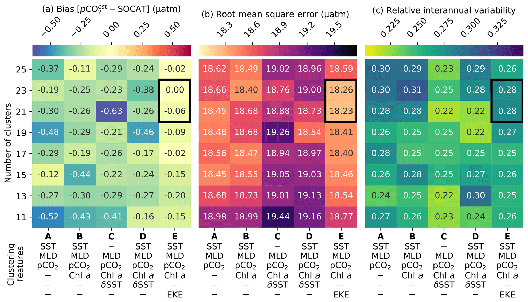
Figure 5 Heat maps showing the average cluster (a) bias, (b) RMSE and (c) relative interannual variability (R^iav) for different cluster configurations, where smaller scores are better for all metrics. The rows show the number of clusters, and the columns show clustering feature-variable configurations. Each cluster contains the average of the scores for four regression methods: support vector regression, extremely randomised trees, gradient-boosting machine and feed-forward neural network. The black box indicates clustering configurations that perform well across all metrics; note that a value of R^iav<0.3 falls within the best category of performance in Rödenbeck et al. (2015).

3 Results

3.1 Regression results

The results from the regression comparisons (step 2 in Fig. 1) are depicted in Fig. 5a–c, which plot the matrix of the (a) average bias, (b) RMSE and (c) R^iav for each combination of the experimental number of clusters and clustering features.

Results show that the configuration that includes EKE^clim (column E in Fig. 5a–c) as a clustering feature has the lowest average RMSE and absolute bias for nearly all clustering configurations, regardless of the number of clusters (rows in Fig. 5a, b). The increased dynamics associated with high-EKE regions might change the way pCO₂ behaves compared to low-EKE regions (Boutin and Merlivat, 2013; Monteiro et al., 2015; du Plessis et al., 2017, 2019). The optimal number of clusters within this configuration is either 21 or 23, based on the smallest bias and RMSE scores (as indicated by the black box in Fig. 5), while we do not weight R^iav strongly in this assessment as a R^iav score of less than 0.3 is in the top-performing category in the SOCOM intercomparison (Rödenbeck et al., 2015). While the individual regression methods' bias and RMSE scores (Figs. S5 and S6, respectively) do not match the distributions exactly, the two selected clustering configurations (black boxes in Fig. 5) score consistently low for both metrics (with the exception of ERT – discussed in greater detail further on). We are motivated to select only one clustering configuration for the sake of simplicity. Furthermore, we select the configuration with 21 clusters (rather than 23), as fewer clusters further reduce the possible complexity at little cost. The selected clustering configuration with 21 clusters has the following features: SST, log₁₀(MLD^clim), $p{\mathrm{CO}}_{\mathrm{2}}^{\mathrm{clim}}$, log₁₀(Chl a^clim) and log₁₀(EKE^clim), and is hereinafter abbreviated as K21E (see Fig. S2 for the distribution of the climatology for these clusters).

Table 3 Regression scores for the CO₂ biomes (BIO23), the clustering configuration from column E in Fig. 5 (K21E) and the ensemble average (CSIR-ML8). Abbreviations are as follows: RMSE is the root mean square error; R^iav is the relative interannual variability (Eq. 5). Regression methods are as follows: SVR is support vector regression; ERT is extremely randomised trees; GBM is the gradient-boosting machine; FFN is the feed-forward neural network. Bold values are significantly lower than the mean for that column (p<0.05 for the two-tailed Z test; absolute values are used for the bias column).

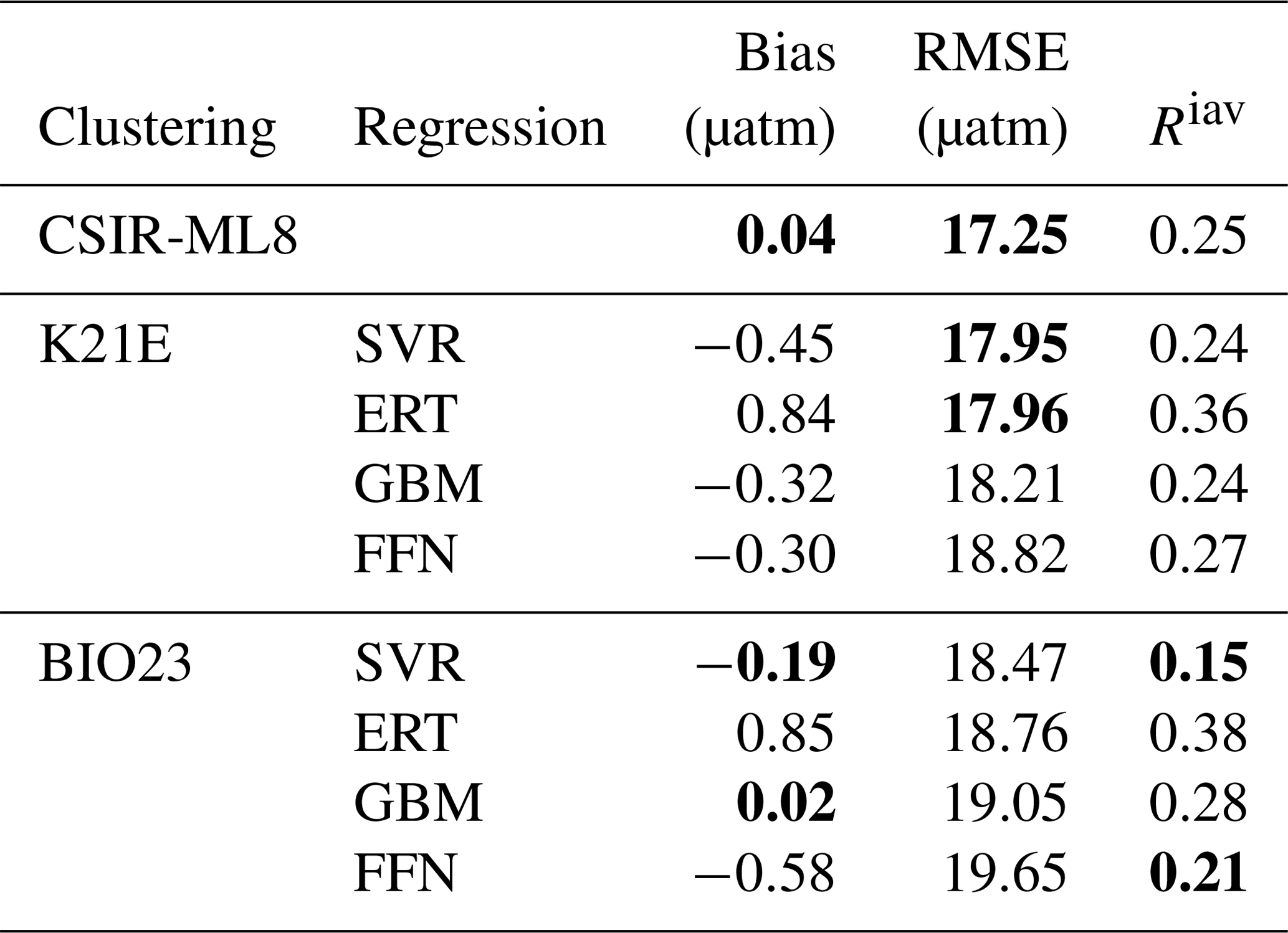
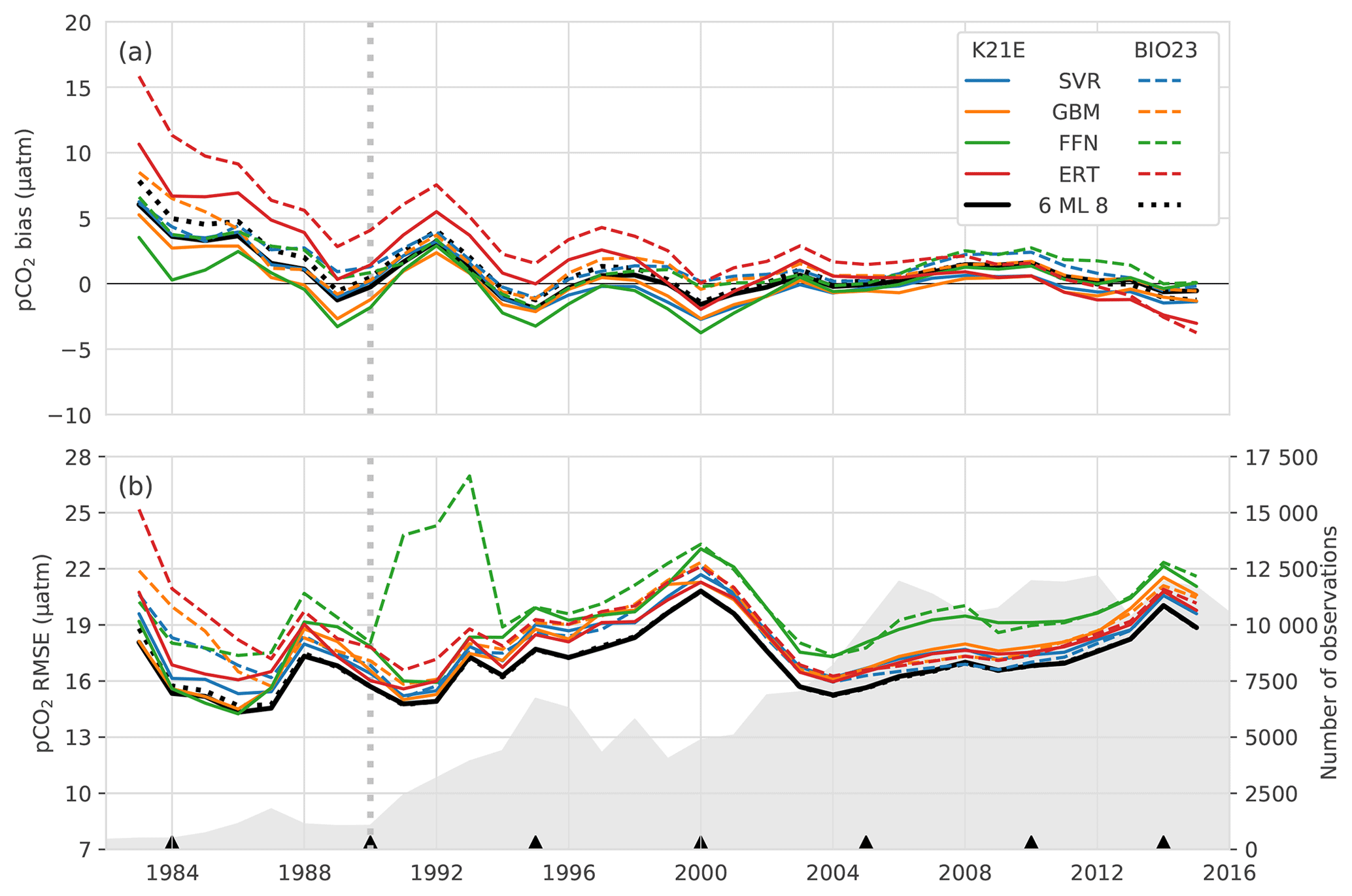
Figure 6 Annually averaged (a) bias and (b) RMSE for the eight individual regression methods in Table 3: BIO23 (dashed lines) and K21E (solid lines). The dotted black lines show the ensemble averages for all eight models (CSIR-ML8), and the solid black line shows metrics for the ensemble average of the SVR, GBM and FFN (CSIR-ML6) from BIO23 and K21E. The grey-filled area in panel (b) shows the number of observations per year, and black triangles show the years that are isolated as the test subset. The vertical dashed grey line demarks 1990, prior to which there is a large positive bias.

Comparatively, the Fay and McKinley (2014) CO₂ biomes have an average RMSE score of 18.98 µatm (Table 3) but have a lower mean R^iav (0.26) and smaller bias (0.03 µatm) than the K21E configuration. Given that the CO₂ biomes perform well and provide an alternate clustering approach, we include the regression estimates. The eight machine-learning models from K21E and BIO23 (four each) were used to create an ensemble average by averaging pCO₂ estimates (CSIR-ML8, Council for Scientific and Industrial Research – Machine Learning ensemble with Eight members).

All regression methods have lower RMSE scores for K21E than for BIO23, but R^iav and bias do not indicate that either of the two clustering approaches is preferable (Table 3). Comparing the RMSE scores of the individual regression methods, we see that the model scores are ranked the same in each cluster from first to last: SVR, ERT, GBM and FFN. However, it is important to note that this ranking does not apply to bias or R^iav, where ERT has low RMSE but the largest bias and R^iav in each clustering approach. CSIR-ML8 only slightly betters its members, with RMSE and bias scores of 17.25 and 0.04 µatm, respectively. However, the ensemble average R^iav (0.25) is only just less than the average of the ensemble members' average (0.26).

Figure 7 Panel (a) shows the biases from the robust test estimates; panel (b) shows the RMSEs for CSIR-ML6. Convolution has been applied to panels (a) and (b) to make it easier to see the regional nature of the biases and RMSE. Figure S8 shows the bias for every ensemble member. Black lines show the regions as defined in Fig. 3.

3.2 Robust RMSE, bias and R^iav

Here, we study the change in the bias and RMSE for all selected methods (i.e. K21E, BIO23 and CSIR-ML8; Table 3) across 1982–2016 (Fig. 6). Most notable is that bias scores for all models have the same interannual tendencies, with a positive bias at the beginning of the time series (1982 to 1993) that is strongest before 1990, strongly influencing the mean bias (Table 4). Secondly, the biases for K21E (solid lines) are, on average, smaller than for BIO23 (dashed lines), as shown for the annually averaged results in Table 4 (0.73 and 2.24 µatm, respectively). These biases are larger than those reported in Table 3 (with averages of absolute biases of 0.48 and 0.41 µatm for K21E and BIO23, respectively), but this is likely since selected test years (black triangles in Fig. 6b) fall on years of low bias. While FFN has the largest RMSE (18.93 and 20.24 µatm for K21E and BIO23), it has a smaller bias compared to other regression methods (0.04 and 1.60 µatm, respectively), motivating including FFN regressions in the ensemble average (Table 4). Conversely, the ERT approach has a significant positive bias likely due to the method's resilience to outliers, where sparse measurements could be treated as outliers (2.08 and 3.88 µatm for K21E and BIO23, respectively, with p>0.95 for both values; Table 4; Gregor et al., 2017). A second ensemble average without ERT regressions, thus with six members (CSIR-MLR6 version 2019a; hereafter called CSIR-ML6), has lower biases compared to CSIR-ML8 (0.98 and 1.48 µatm, respectively; Table 4).

Similar to the biases, RMSEs for all models (Fig. 6b) have similar interannual tendencies and variability, with a sharp peak in the year 2000 (> 20 µatm, where the mean RMSE is 18.61 µatm). The increased RMSE scores are likely due to the spatial distribution of sampling density (see Fig. S7); e.g. an increase in sampling in the high latitudes during spring and summer, a region and period of high variability and biogeochemical complexity, would increase the weight of these data in the final RMSE calculation, thus resulting in larger RMSE scores. The increase in the number of samples from 2002 to 2016 results in a sharp decrease in RMSE (< 19 µatm for the majority of this period). Both ensemble averages perform slightly better than all other methods for the majority of the time series with RMSE scores of 17.16 and 17.25 µatm for CSIR-ML6 and CSIR-ML8, respectively (see Table S1 comparisons of ensemble averages with different members).

Table 4 The robust estimates of bias, RMSE and R^iav from 1982 to 2016 for BIO23, K21E and the ensemble averages, CSIR-ML6 and CSIR-ML8, where the first excludes the ERT method. Bold values are significantly lower than the mean for that column (p<0.05 for the two-tailed Z test; absolute values are used for the bias column). See Table S1 for further comparisons between different ensemble average configurations.

The R^iav scores for the robust errors (Table 4) are lower than train-test results with a single split reported in Table 3, likely due to an increase of standard deviation for the IAV benchmark (Eq. 5). The lowest score is held by CSIR-ML6 (0.20) and is lower (better) than the average for its members (0.21). These R^iav estimates compare well to the Jena-MLS and SOM-FFN, which both scored < 0.3 (Rödenbeck et al., 2015).

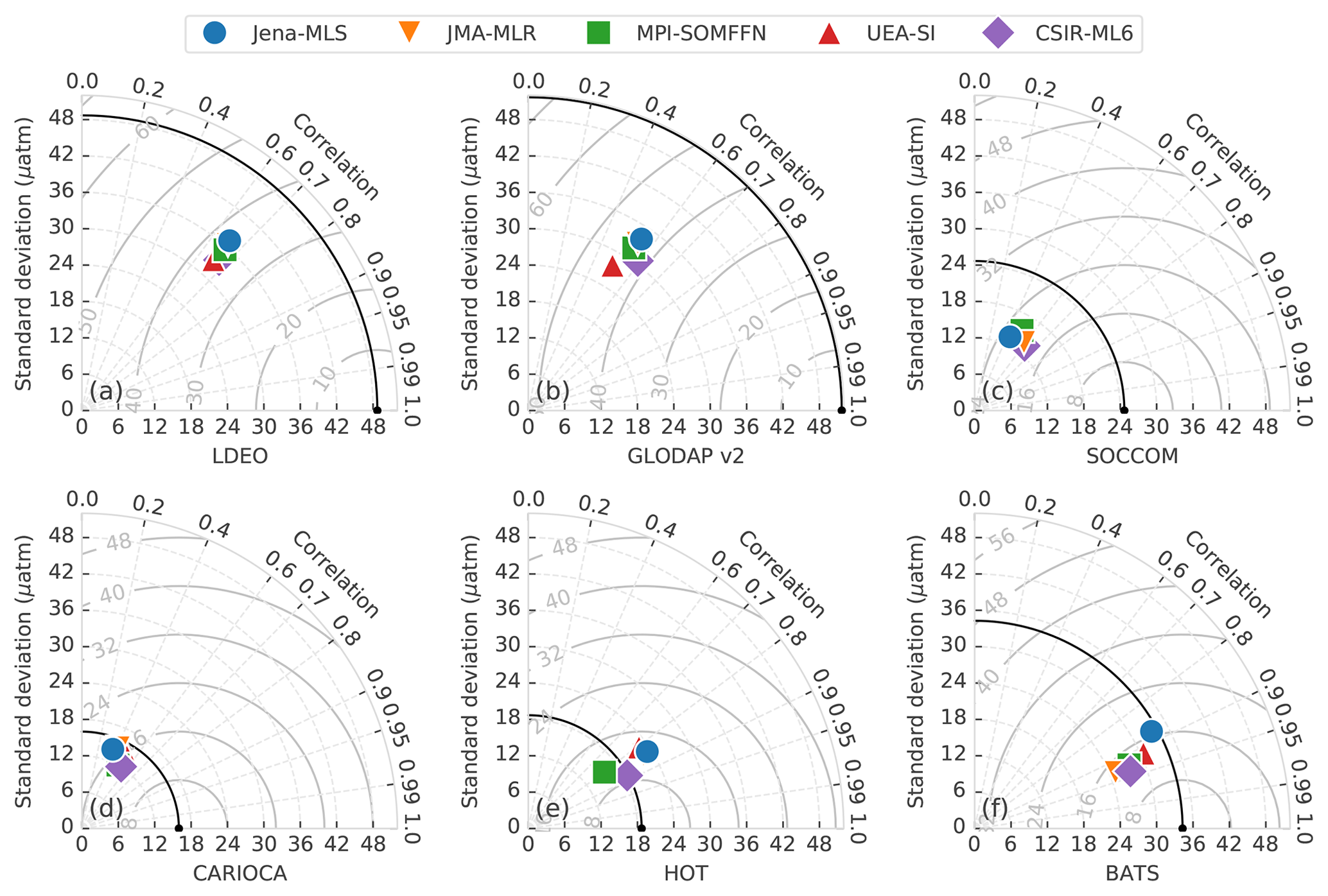
Figure 8 Taylor diagrams comparing the pCO₂ estimates of five gap-filling methods (represented by the different markers) with validation datasets (Table 2) for the period 1990–2015. Each validation dataset has its own Taylor diagram, as labelled on the bottom axes. The black marker on the bottom axis in each subplot represents the validation dataset and the black arc shows the standard deviation thereof. The closer the gap-filling estimates are to this point, the better the model's performance, in terms of variance, centred RMSE and correlation (for bias information, see Table 5). The solid grey arcs show the centred RMSE for the datasets (with bias removed). A description of the gap-filling methods from independent studies is provided in the text (Sect. 3.3).

The spatial distribution of the bias and RMSE is now studied for CSIR-ML6 (Fig. 7a and b, respectively), particularly focusing on the regional patterns emerging from the data. CSIR-ML6 clearly represents the subtropical regions (NH-ST and SH-ST) with relatively low biases and RMSE scores (|bias| < 5 µatm and RMSE < 10 µatm). The equatorial regions (EQU), especially the eastern Pacific, contrasts this with large uncertainties in both bias and RMSE (> |10 µatm| and 30 µatm, respectively). The high-latitude oceans (NH-HL and SH-HL) have considerable uncertainties due to the large interannual variability of surface ocean pCO₂ caused by the formation and retreat of sea ice (around Antarctica; Ishii et al., 1998; Bakker et al., 2008) and phytoplankton spring blooms (Atlantic sector of the Southern Ocean, North Pacific and Arctic Atlantic; Thomalla et al., 2011; Lenton et al., 2013; Gregor et al., 2018). There are two bands of overestimates on the southern and northern boundaries of the North Atlantic Gyre, where the latter coincides with the Gulf Stream. Regression approaches may be prone to a positive bias in the North Atlantic, as this was also shown by Landschützer et al. (2013, 2014).

In summary, the robust test estimates show that there is a positive bias in pCO₂ predictions before 1990 for all models, but it is largest for ERT, and excluding these models from the ensemble results in better pCO₂ predictions. The spatial evaluation of the performance metrics for CSIR-ML6 shows that regions with specific oceanic features (e.g. western boundary currents) mostly have positive biases. However, it is important to note that these uncertainty assessments are limited as the characteristics and biases of the dataset are intrinsic to the models. Validation with independent data is thus a more reliable estimate of the performance of these methods.

3.3 Validation with independent datasets

Here, we validate the accuracy of pCO₂ estimates from CSIR-ML6 with independent data (that are not in SOCAT v5, as described in Table 2). To further study the behaviour of our ensemble average estimates relative to previous studies, we compare the results from four independent methods of the SOCOM intercomparison project against the independent data calculated over individual data points (Rödenbeck et al., 2015). Those four independent methods are the Jena mixed-layer scheme (Jena-MLS version oc_v1.6; Rödenbeck et al., 2014); JMA-MLR, updated on 2 December 2018 (Iida et al. 2015); MPI-SOMFFN v2016 (Landschützer et al., 2017); and University of East Anglia – Statistical Interpolation (UEA-SI version 1.0; Jones et al., 2015). pCO₂ estimates by the Jena-MLS were resampled to monthly temporal resolution and interpolated to a 1^∘ grid using Python's xarray package. Note that these datasets will also suffer from the same temperature biases discussed in Sect. S2.4.

The performance of each gap-filling method is represented with a Taylor diagram for each independent validation dataset (Fig. 8; Taylor, 2001). The most important characteristic learnt from these plots is that the gap-filling methods are tightly bunched for nearly all validation datasets, indicating a similar RMSE, correlation and standard deviation relative to the reference datasets. Poor estimates in Fig. 8a–d may indicate that the training data for gap-filling methods is the limiting factor. Secondly, the gap-filling methods almost always underestimate the standard deviation of the validation datasets, being below the black arched line for all but the station HOT (Fig. 8e).

Table 5 The RMSE and bias for each gap-filling method compared to the validation datasets. For more information on the validation datasets, see Table 2. The first row of data (count) shows the number of gridded samples in the dataset during the period 1990–2015 (that are not in the SOCAT v5 gridded product). Values shown in bold are significantly different from the mean for the column (p<0.05 for the two-tailed Z test; absolute values are used for the biases). The UEA-SI method does not have error estimates for SOCCOM floats as these two time series do not overlap.

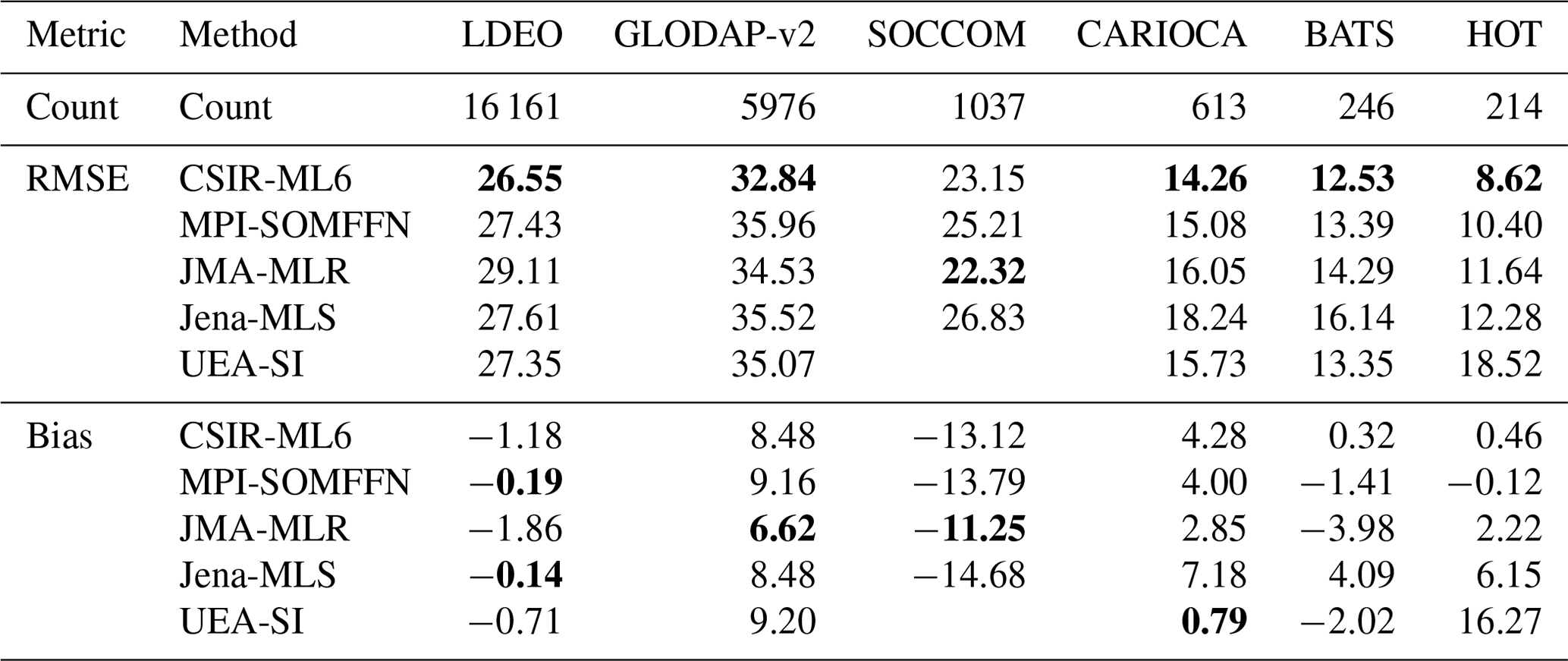
All methods fail to represent the standard deviation of the two global validation datasets, LDEO and GLODAP v2 (Fig. 8a, b), with centred RMSE scores greater than 35 µatm. However, calculating RMSE annually results in scores of ∼ 27 µatm for LDEO and ∼ 35 µatm for GLODAP v2, much lower than shown in Fig. 8a–b, due to high RMSE scores (> 40 µatm) for a small subset of years (Sect. S3.4 and Fig. S7). Estimates of the Southern Ocean datasets (Fig. 8c, d), SOCCOM and CARIOCA, have lower RMSE scores (∼ 16 and ∼ 23 µatm, respectively) relative to LDEO and GLODAP v2. However, for standard deviation scores of similar magnitude and low correlation coefficients, the datasets are not well constrained (Table 5). The SOCCOM dataset also has the largest average absolute bias for estimates, with gap-filling methods underestimated by at least 11 µatm (Table 5). This large bias may be because SOCCOM floats have a proportionately large number of winter samples – suggesting that our knowledge of Southern Ocean winter fluxes is largely underestimated (Williams et al., 2017). In contrast, all methods estimate the two time series stations, HOT and BATS (Fig. 8e, f and Table 5), relatively well with correlation scores > 0.8 and low average bias ∼ 4.5 µatm.

Despite all scores being closely grouped (Fig. 8), Table 5 shows that the CSIR-ML6 method scores significantly lower RMSE scores (using a two-tailed Z test with p<0.05) for all but one of the datasets (SOCCOM). However, bunching of the RMSE scores (Fig. 8) is beneficial with regard to achieving low p values. No single method dominates the biases, with JMA-MLR and MPI-SOMFFN each scoring the lowest bias on two occasions. To summarise, all gap-filling methods underperform when validated against independent observational products. Tight bunching of gap-filling method scores per validation dataset shows that training data may limit all methods in the same manner.

Figure 9 (a) Average sea–air CO₂ fluxes (FCO₂) of CSIR-ML6 for 1990 to 2016, where FCO₂ is calculated as shown in Eq. (2). Negative FCO₂ (blue) indicates regions of atmospheric CO₂ uptake. (b) The differences between FCO₂ in 2016 and 2000, which are the minimum and maximum of global ocean uptake flux (FCO₂) estimates, respectively (for CSIR-ML6 in Fig. 10a). Black lines show the regions as defined in Fig. 3.

3.4 The effect of uncertainties on the sea–air CO₂ flux interannual variability

In this section, we assess the regional implications of the differences in gap-filling methods' estimates (within CSIR-ML6 and the four independent methods described in Sect. 3.3) of the sea–air CO₂ flux (FCO₂) over the period 1990 to 2016. FCO₂ was calculated using the same gas-transfer velocity and solubility for each gap-filling method (Sect. 2.7). Differences in FCO₂ are thus driven by variations in pCO₂ from each gap-filling method.

The average FCO₂ for 1990–2016 by CSIR-ML6 (Fig. 9a) contextualises the regional distribution of fluxes: strong outgassing in the equatorial Pacific, strong sink in the midlatitudes, a moderate uptake for the most part of the subtropics and weak source in the majority of the Southern Ocean (in agreement with, e.g. Takahashi et al., 2009). The global annual time series for FCO₂ as simulated by CSIR-ML6 (Fig. 10a) indicates a strengthening for 2000 to 2016 (as for the other methods). To give spatial context to this strengthening, we display the differences in FCO₂ between 2016 and 2000 (Fig. 9b), since those are the two years where the difference in global FCO₂ is greatest for CSIR-ML6 (Fig. 10a). Note that Fig. 9b serves as a snapshot for the change in FCO₂ between those two years, whose interpretation cannot be linked to an overall anthropogenically forced change as the comparison between the two years could reflect interannual, decadal or multi-decadal variability. The differences in FCO₂ between 2016 and 2000 are negative in the high latitudes and moderately positive in the subtropics, indicating a respective increase and decrease in the CO₂ ocean uptake between the two years. The eastern equatorial Pacific is the only region that shows a considerable increase in FCO₂ (> 10 g C m⁻² yr⁻¹) between the two specific years.

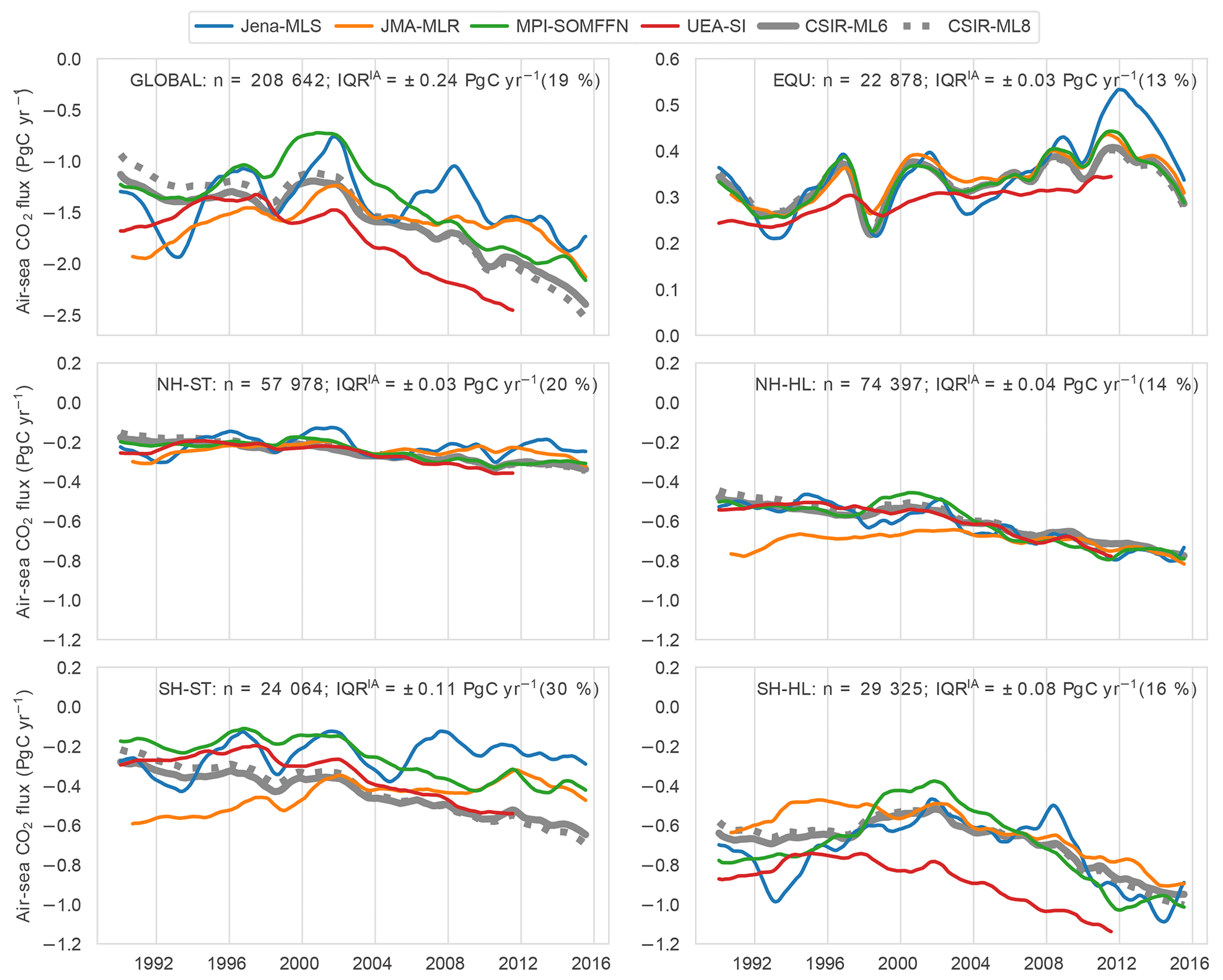
Figure 10 Sea-air CO₂ fluxes averaged for regions as shown in Fig. 2: (a) global domain, (b) equatorial regions, (c) Northern Hemisphere subtropical, (d) Northern Hemisphere high latitude, (e) Southern Hemisphere subtropical. (f) Southern Hemisphere high latitude. The coloured lines show the four SOCOM products. The thick and dotted grey lines show the results for CSIR-ML6 and CSIR-ML8, respectively. A moving average of 12 months has been applied to smooth the data. Note that the y-axis scales differ for the top (a, b). Note that the uncertainties of each model (e.g. bias and RMSE from Fig. 6) are not shown here. The text at the right of each figure shows the number of SOCAT v5 gridded data points for each region (n) and the interannual interquartile range (IQR^IA).

The annual change in FCO₂ is also studied for the different regions. The Southern Hemisphere high-latitude (SH-HL) region is the strongest contributor to the trend (Fig. S10b), where there is a steady increase in the uptake of CO₂ since the 2000s for all methods (Landschützer et al., 2015; Gregor et al., 2018). On average, the Northern Hemisphere high latitudes (NH-HL) are a weaker sink relative to the SH-HL, because the SH-HL is more than double the area of the NH-HL (Fig. S10c). The equatorial (EQU) region is the only persistent source of CO₂ to the atmosphere (also seen in Fig. 9a). The subtropical regions (Fig. 10c, e) contribute to global flux on similar orders of magnitude; however, there is a large divergence between gap-filling methods in the SH-HL.

We use the average interquartile range between the 1-year rolling mean estimates (IQR^IA) as a measure of agreement or divergence between gap-filling methods, where large values indicate a divergence (Sect. 2.8.2). We also show the IQR^IA scaled to the range of the regional interannual variability (max–min) as a percentage (relative IQR^IA), which shows if the trend for a particular region is agreed on by all methods (the smaller the percentage, the better the agreement across methods). The disagreement between methods in the SH-ST is substantial (Fig. 10e), with diverging FCO₂ throughout the period with an IQR^IA of 0.11 Pg C yr⁻¹ and a large relative IQR^IA of 28 %. Similarly, the IQR^IA for the SH-HL region (Fig. 10f) is 0.08 Pg C yr⁻¹, but the relative IQR^IA is lower at 14 %, indicating that all methods agree on the observed strong trend. Compared to the Southern Hemisphere, the Northern Hemisphere regions are both relatively well constrained, with IQR^IA estimates of 0.04 and 0.05 Pg C yr⁻¹ for the NH-ST and NH-HL regions, respectively (Fig. 10c, d). However, a larger relative IQR^IA of 20 % suggests that the interannual FCO₂ estimates in the NH-ST region are potentially not resolving the trend, or more likely that there is a weak trend with a small difference between the minimum and maximum interannual estimates of FCO₂. The EQU region (Fig. 10b) has an IQR^IA and relative score at 0.03 Pg C yr⁻¹ and 14 %.

The CSIR-ML8 method is not included in the IQR^IA calculations but is included in Fig. 10 to show the impact of the ERT models' positive bias in pCO₂ on FCO₂ (Fig. 6a). The biases are positive at the beginning and negative end of the time series, with the average absolute difference between the CSIR methods being 0.08 Pg C yr⁻¹. The positive biases have the strongest impact on the SH-ST that occupies 36 % total area (Fig. S10c), with only 11 % of the total observations in SOCAT, suggesting that this method is sensitive to imbalanced datasets.

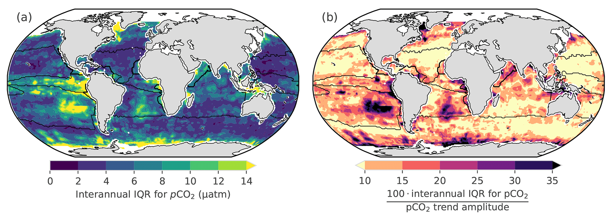
Figure 11 (a) The magnitude of the interannual disagreement between independent gap-filling methods (IQR^IA) as shown in Fig. 10; hence, low IQR^IA indicates good agreement amongst the different methods. (b) Level of agreement on the interannual variability across methods (in %), more specifically IQR^IA scaled by the difference between the maximum and minimum values for interannual pCO₂ (the range).

3.5 Regional disagreement between methods

In order to better understand the regional distribution of the uncertainties in FCO₂, we assess the level of agreement between independent gap-filling methods in their interannual surface ocean pCO₂ estimates (Fig. 11). We use pCO₂ for this representation as no spatial integration occurs – only time averaging.

The interannual estimates of IQR^IA (Fig. 11a) show the disagreement between methods is relatively small in the majority of the ocean (< 6 µatm), with the exceptions being the Southern Ocean, South Atlantic, southeastern Pacific and eastern equatorial Pacific with differences of > 10 µatm, where these regions coincide with regions of low sampling density (Fig. 2). The IQR^IA scaled to the maximum–minimum range of interannual pCO₂ suggests that the NH-ST trend is relatively well constrained (< 10 %), which is in conflict with the IQR^IA for FCO₂ in Fig. 10c (where the relative IQR^IA is 20 %). The disagreement may stem from the magnifying impact that wind speed has on FCO₂; i.e. small differences in pCO₂ may become large when fluxes are calculated. The same principle may apply to the EQU in Fig. 11b, where relative IQR^IA is large (> 10 %) for pCO₂, but low wind speeds result in a low relative IQR^IA for FCO₂ (7 % in Fig. 10b). The largest relative IQR^IA scores occur in the SH-ST (> 10 % in Fig. 11c) where data are sparse, specifically the South Atlantic and southeastern Pacific (Fig. 2a). The relative IQR^IA scores suggest that the gap-filling methods agree on pCO₂ in the SH-HL east of the Greenwich meridian (> 0^∘ E).

In summary, we show that there is an agreement between gap-filling methods in the Northern Hemisphere for interannual pCO₂, but the methods show considerable disagreement in the Southern Hemisphere, particularly in the subtropics. Disagreements in the equatorial and Southern Hemisphere high-latitude regions are large (> 10 %) and should be treated with caution when considering trends in these regions.

4 Discussion

4.1 Not all models are equal

In their study, Khatiwala et al. (2013) stated that “our comparison of different methods suggests, that multiple approaches, each with its own strengths and weaknesses, remain necessary to quantify the ocean sink of anthropogenic CO₂”. In our study, we embrace this philosophy by creating an ensemble average of two-step machine-learning models that estimate global surface ocean pCO₂. We show robustly that the CSIR-ML6 method reproduces the available data with greater accuracy than previous methods, albeit in an incremental way. Our method is methodologically consistent with regard to feature variables. Though there is variability in the clustering and regression, we create the ensemble average with a good understanding of each model's biases (Figs. 6 and S8). The argument that ensemble averages reduce transparency is also somewhat diminished by the fact that little additional information that can be gained from highly non-linear models, with the exception of basic diagnostics such as feature-variable importance (see Fig. S11) from decision-tree-based approaches (Pedregosa et al., 2011; Castelvecchi, 2016). Our results thus show that there is, in fact, a benefit in creating an ensemble average of models (Table 5), and if carefully implemented, it is an additional tool that can be used to reduce the uncertainties in gap-filling estimates of pCO₂.

It could be argued that an exhaustive search for the optimal configuration (Fig. 5) for CSIR-ML6 may result in poorly trained individual models. However, we think that the merit of introducing and assessing regression algorithms new to the application (for gradient-boosting machines and extremely randomised trees) outweighs the marginal loss in potential performance for individual methods. Moreover, lessons learnt from our study can be used to improve on future iterations. It also makes the case for ensemble averages stronger, as the CSIR-ML6 performs well relative to other gap-filling methods.

In the search for the optimal clustering configuration (Fig. 5a, b), we show that including EKE (along with SST) as a clustering feature variable leads to an improvement in bias and RMSE for nearly all numbers of clusters, albeit a small improvement. Increased intraseasonal variability of pCO₂ appears to be associated with regions of high EKE compared to low EKE regions (Monteiro et al., 2015; du Plessis et al., 2017, 2019). Moreover, the importance of EKE as a part of the clustering constraints also shows that more thought should be given to how we sample pCO₂ in high-EKE regions and at what resolution regression methods are run at.

Our findings suggest the following about the individual regression methods: the SVR and GBM algorithms produce good estimates with lower RMSE scores and biases, the FFN approach has larger RMSE scores yet low biases than the other methods, and the ERT approach has low RMSE scores but large biases in the estimates (Fig. 6a, b; Table 4). We do not include the ERT approach in the ensemble average (CSIR-ML6) due to the large time-evolving biases, suggesting that ERT (with our tuning) is not suitable for estimating surface ocean pCO₂. The bias in ERT may be due to its sensitivity to imbalanced datasets (Crone and Finlay, 2012), where the data in SOCAT v5 are sparse before 2000. Returning to the above quote by Khatiwala et al. (2013), we thus find that the weaknesses of ERT outweigh its strengths.

4.2 Divergent gap-filling estimates

While we see that the improvements in the performance of gap-filling methods are relatively stagnant (relative to the training and validation data), the differences between the methods' estimates of pCO₂ and FCO₂ vary significantly in some regions, particularly in regions where data are sparse, such as in the Southern Hemisphere oceans (Fig. 2). We also find that training the gap-filling methods with limited training data exposes the intrinsic biases of the algorithms, or in the words of Ritter et al. (2017): “the difference [between gap-filling methods] is a result of how the spatial and seasonal heterogeneity and the sparseness of the data is dealt with”. Conversely, as the number of training data increases, the biases are reduced, and the methods converge.

The Northern Hemisphere subtropical regions are a good example of a region where the gap-filling methods converge (Fig. 11b), as also shown by the low RMSE scores and high correlation for the two mooring stations, HOT and BATS (Fig. 8e, f). One of the reasons that the methods predict the variability well in the subtropics (Fig. 8e, f) is that these regions are less biogeochemically complex and driven primarily by seasonal changes in SST (Bates, 2001; Dore et al., 2009). This strong SST-driven seasonality in the subtropics is shown by the high seasonal cycle reproducibility (Fig. 12).

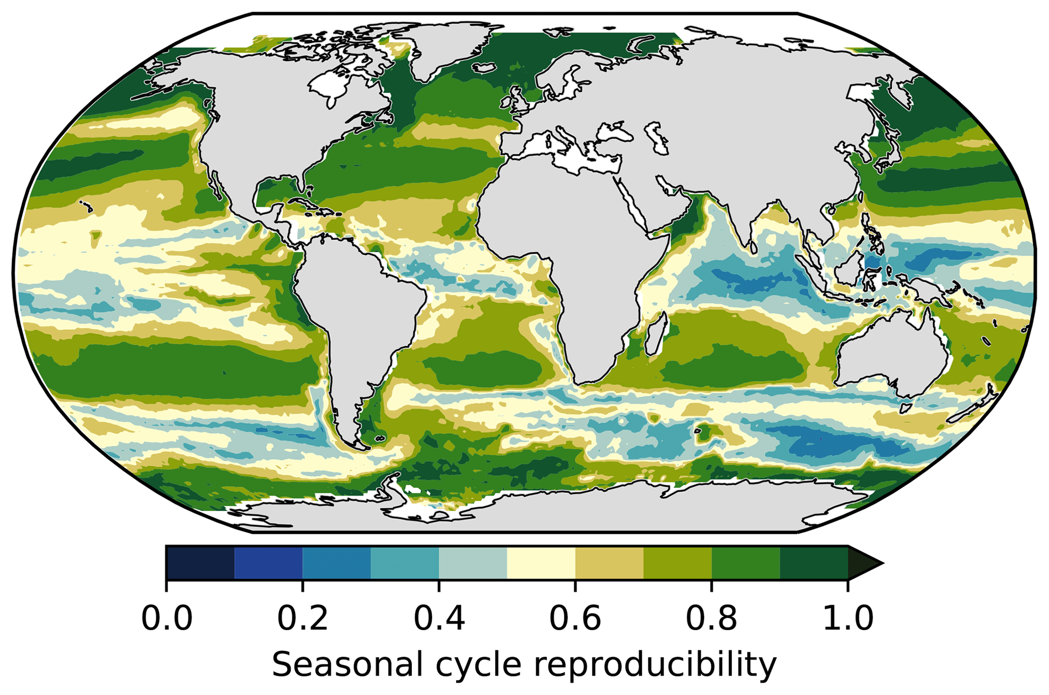
Figure 12 The seasonal cycle reproducibility of CSIR-ML6 pCO₂, which is a correlation of detrended pCO₂ with its own climatology – the larger the correlation, the stronger the reproducibility of the seasonal cycle (method from Thomalla et al., 2011).

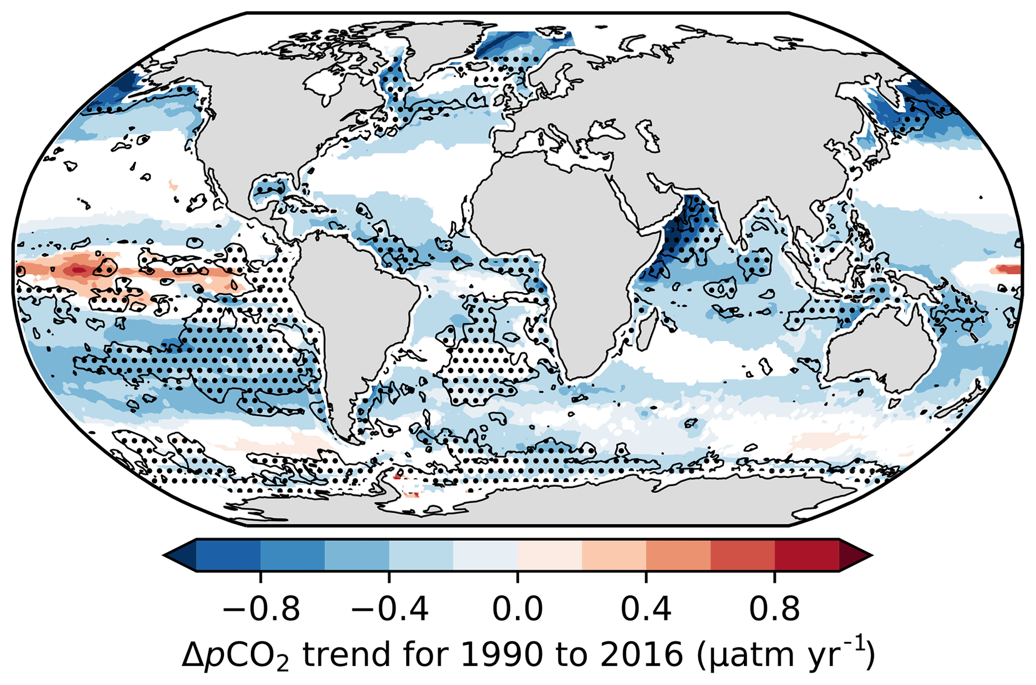
Figure 13 ΔpCO₂ trends (p<0.05), where ΔpCO₂ is calculated as the estimated surface ocean pCO₂ from the CSIR-ML6 method minus atmospheric pCO₂ from the CarboScope project (Rödenbeck et al., 2014). The shaded areas show the regions where IQR^IA is > 15 %, thus indicating regions where trends should be interpreted with caution.

The gap-filling methods' divergences also serve as a metric to inform where there are not enough data to constrain the pCO₂ or FCO₂ estimates; i.e. the divergences inform us where estimates should be treated with caution. The IQR^IA, when scaled to the range of interannual variability (Fig. 11b), should be taken into account when analysing interannual trends of ΔpCO₂ (Fig. 13). For instance, significant trend estimates in ΔpCO₂ for CSIR-ML6 (p<0.05) are negative for the majority of the global ocean, even in regions where method estimates are too disparate to resolve interannual variability (relative IQR^IA>15 %; dotted regions in Fig. 13). However, the relative IQR^IA is not without its limits, as there may be regions where methods are in agreement but share the same biases, thus reporting false confidence in the estimates. Regions of false confidence would most likely occur in data-sparse areas but could only truly be identified with better data coverage in these regions.

4.3 Inching up and over the wall: incremental improvements

In our study, we show that all gap-filling methods suffer from the same uncertainties where there are data to test and validate the estimates (Fig. 8), and result in divergences between estimates when there are insufficient data to constrain the methods (Fig. 11b). From these points, it may seem that we may have in fact “hit the wall” in terms of better resolving surface ocean pCO₂. In this section, we discuss how we might overcome this proverbial wall: first, by addressing the existing uncertainty and biases, and then discussing how we could improve on estimates in data-poor regions.

4.3.1 Reducing existing biases

The robust test estimates show that there are regions where training data are not sparse, yet estimates still suffer from large uncertainties (e.g. northern and southern boundaries of the North Atlantic Gyre in Figs. 7a, b and S8). These errors are spatially consistent with those reported by Landschützer et al. (2014). Such regional mismatches between gridded observations and estimates are likely systematic – meaning that gap-filling methods are not able to resolve the more complex pCO₂ variability at current resolutions (monthly × 1^∘ or coarser) or with the current regression feature variables (Gregor et al., 2017; Denvil-Sommer et al., 2018). It may be possible to reduce these uncertainties with consideration about the drivers of CO₂ in a specific region. Including appropriate additional feature variables (if available), such as reanalysis mixed-layer depth products, may improve the uncertainties of gap-filling methods (Gregor et al., 2017). Similarly, increasing the temporal and spatial resolution may be able to improve estimates where aliasing occurs in regions of high dynamic variability such as the midlatitude oceans (Monteiro et al., 2015). It is worthwhile to note that increasing the resolution may not be the panacea for poor estimates. For example, the Jena-MLS method is able to estimate pCO₂ with relative accuracy (Fig. 8) at a low spatial resolution ($\approx {\mathrm{4}}^{\circ }\times {\mathrm{5}}^{\circ }$; Rödenbeck et al., 2014); however, with the trade-off in spatial resolution, the method is able to increase the temporal resolution to daily estimates.

Another source of bias is the mismatch between the temperature at which pCO₂ is measured (i.e. at the depth of a ship's intake) and the temperature to which pCO₂ is predicted (∼ 1 m in the case of the dOISSTv2 data; Banzon et al., 2016; Goddijn-Murphy et al., 2015). Goddijn-Murphy et al. (2015) show that this mismatch is considerable in some cases (> 5 µatm for large regions, as shown in Fig. S3b). However, the correction of the intake temperature to the remotely sensed surface temperature also makes the assumption that temperature is the only factor that influences pCO₂ in the surface layer of the ocean. The correction will thus not account for other processes such as primary production, stratification and gas exchange within the surface layer. This is an issue that should be discussed by the community and tested experimentally to assess the impact that these processes may have on pCO₂.

4.3.2 Improving estimates in data-poor regions

All gap-filling methods suffer from similar biases and uncertainties (Fig. 8, Table 5) when compared to independent validation data, yet the same methods show vastly different results in data-sparse regions. These shared uncertainties and regionally consistent divergences between methods are in agreement with past studies, which find that insufficient training data are the limiting factor (Rödenbeck et al., 2015; Landschützer et al., 2016; Ritter et al., 2017; Denvil-Sommer et al., 2018).

Strides have been made in closing these data-sparse gaps with the deployment of autonomous sampling platforms. The SOCCOM project, in particular, has been influential in closing the gap in the Southern Ocean with the deployment of ∼ 200 pH-capable biogeochemical Argo floats in the region since 2015 (Williams et al., 2017; Gray et al., 2018). The data collected by these floats during winter have shown that we have previously underestimated winter outgassing of CO₂ in the Southern Ocean (Gray et al., 2018). Incorporating these new estimates into machine-learning estimates should be a priority for the community as the Southern Ocean plays an important role in anthropogenic CO₂ uptake (Gruber et al., 2019). Incorporating these data successfully into existing models may not be straightforward due to the strong temporal bias of these data toward the end of the time series. For instance, the inclusion of atmospheric pCO₂ could result in temporally skewed estimates due to the “memory” effect that including the annually increasing atmospheric pCO₂ could have on estimates.

The complex machine-learning models often used to estimate pCO₂ are prone to overfitting the data, particularly in regions where data are sparse. Using less complex models, e.g. multi-linear regression, in such regions would reduce the risk of overfitting the data. A regionally weighted ensemble approach may be an eloquent way to address this problem. In regions with sparse data coverage, simpler models could be favoured, while more complex models could be weighted more in regions with more data. However, the user would have to apply a potentially subjective model-complexity ranking for each approach. This may work well in the subtropical gyres where pCO₂ has a strong seasonal signal driven primarily by temperature (Fig. 12; Taylor, 2001).

One of the weaknesses of our study is that our approach is similar to other regression methods (e.g. MPI-SOMFFN by Landschützer et al., 2014, and JMA-MLR and LSCE-FFNN by Denvil-Sommer et al., 2019) that predict pCO₂ based on the instantaneous physical and biological variables without regard for past states. There is thus a need to explore methods that incorporate the past state into future state estimates. This includes assimilative modelling approaches, such as B-SOSE (biogeochemical Southern Ocean state estimate), which would also provide greater understanding of the driver for changes in surface pCO₂ (Verdy and Mazloff, 2017). These methods may be able to provide better constraints on pCO₂ in data-poor regions. However, these assimilative models are not yet in a stage to fit the data closely (Verdy and Mazloff, 2017).

5 Summary

Our study suggests that we may be reaching the limits of gap-filling methods' abilities to reduce uncertainties, as shown by the limited incremental improvement in errors by the ensemble method we compare with established methods. Significant uncertainties still prevail across all gap-filling methods, most likely limited by the extent of basin-scale observational gaps in the Southern Hemisphere as well as sampling aliases in mesoscale intensive ocean regions. We propose ways in which the surface ocean CO₂ community can improve estimates within the bounds of the current observations and make recommendations for future observations.

We introduce a new surface ocean pCO₂ gap-filling method that is a machine-learning ensemble average of six two-step clustering-regression models (CSIR-ML6 version 2019a). An exhaustive search process was used to find the best K-means clustering configuration which was used alongside the Fay and McKinley (2014) oceanic CO₂ biomes. The regression models applied to each clustering method are support vector regression, feed-forward neural networks and gradient-boosting machines. We show that the ensemble average of the six methods marginally outperforms each of its members, thus promoting the idea that averaging model estimates, each with different strengths and weaknesses, result in an improvement in the overall estimates.

The CSIR-ML6 (version 2019a) approach was compared to validation data alongside four other methods from the SOCOM intercomparison study (Rödenbeck et al., 2015). Our new method marginally outperformed the SOCOM methods when comparing RMSE scores for the validation data but fared equally on biases. Despite this improvement, all methods had errors of roughly the same magnitude, suggesting that the methods resolve pCO₂ equally outside the bounds of the training data.

Closer assessment of the spatial distribution of errors shows that there is spatial coherence between regression approaches for the Northern Hemisphere. Some of these errors coincide with regions of high dynamic variability or complex biogeochemistry, suggesting that increasing the spatial and temporal resolution of gap-filling methods could improve estimates. Moreover, introducing additional feature variables for regression, such as eddy kinetic energy, may improve estimates in these regions.

A comparison of the distribution of mismatches in pCO₂ between gap-filling methods shows that there are regions (primarily in the Southern Hemisphere) where the compared methods, as an ensemble, cannot resolve interannual variability of pCO₂ and as such, trends analyses in those regions should be interpreted with caution. These large mismatches likely occur due to amplification of algorithm specific biases in data-sparse areas. We suggest that an ensemble with data-density-driven weighting for model complexity could be a way to reduce potential overfitting in data-sparse regions. We also urge the community to focus on incorporating new measurements from autonomous platforms such as the pCO₂ derived from pH measured by biogeochemical Argo floats and new platforms such as pCO₂-capable Wavegliders.

In closing, we suggest that it is time to consider another SOCOM-like intercomparison. Several new methods have been developed since the last intercomparison and the addition of these would improve the robustness of ensemble average flux estimates. Further, the authors of the SOCOM intercomparison suggest that a future intercomparison should include a comparison of methods using simulated data, a method to overcome the limitation of the lack of data to test the estimates.