the Creative Commons Attribution 4.0 License.
the Creative Commons Attribution 4.0 License.
 | 03 Dec 2019
Improving the LPJmL4-SPITFIRE vegetation–fire model for South America using satellite data
Matthias Forkel
Werner von Bloh
Boris Sakschewski
Manoel Cardoso
Mercedes Bustamante
Jürgen Kurths
Kirsten Thonicke
Vegetation fires influence global vegetation distribution, ecosystem functioning, and global carbon cycling. Specifically in South America, changes in fire occurrence together with land-use change accelerate ecosystem fragmentation and increase the vulnerability of tropical forests and savannas to climate change. Dynamic global vegetation models (DGVMs) are valuable tools to estimate the effects of fire on ecosystem functioning and carbon cycling under future climate changes. However, most fire-enabled DGVMs have problems in capturing the magnitude, spatial patterns, and temporal dynamics of burned area as observed by satellites. As fire is controlled by the interplay of weather conditions, vegetation properties, and human activities, fire modules in DGVMs can be improved in various aspects. In this study we focus on improving the controls of climate and hence fuel moisture content on fire danger in the LPJmL4-SPITFIRE DGVM in South America, especially for the Brazilian fire-prone biomes of Caatinga and Cerrado. We therefore test two alternative model formulations (standard Nesterov Index and a newly implemented water vapor pressure deficit) for climate effects on fire danger within a formal model–data integration setup where we estimate model parameters against satellite datasets of burned area (GFED4) and aboveground biomass of trees. Our results show that the optimized model improves the representation of spatial patterns and the seasonal to interannual dynamics of burned area especially in the Cerrado and Caatinga regions. In addition, the model improves the simulation of aboveground biomass and the spatial distribution of plant functional types (PFTs). We obtained the best results by using the water vapor pressure deficit (VPD) for the calculation of fire danger. The VPD includes, in comparison to the Nesterov Index, a representation of the air humidity and the vegetation density. This work shows the successful application of a systematic model–data integration setup, as well as the integration of a new fire danger formulation, in order to optimize a process-based fire-enabled DGVM. It further highlights the potential of this approach to achieve a new level of accuracy in comprehensive global fire modeling and prediction.
- Article
(5112 KB) - Full-text XML
- BibTeX
- EndNote


Fire in the Earth system is an important disturbance leading to many changes in vegetation and has a substantial impact on biodiversity, human health, and ecosystems (Langmann et al., 2009). Fire is responsible for ca. 2 Pg of carbon emission, which constitutes 20 % of global carbon emission (Giglio et al., 2013; van der Werf et al., 2010). Fire-induced aerosol emissions and land-surface changes modify evapotranspiration and surface albedo and therefore have a crucial impact on global climate (van der Werf et al., 2008; Yue and Unger, 2018). Despite a tendency for globally declining burned area (Andela et al., 2017; Forkel et al., 2019b), more frequent and intense drought periods lead to increasing fire-prone weather and surface conditions worldwide, and therefore fire danger (Jolly et al., 2015). Growing fire danger and land-use change are increasing the ecosystem's vulnerability, which could in turn shift entire regions into a less vegetated state (Silverio et al., 2013). To account for these effects, it is extremely important to include well performing fire modules in dynamic global vegetation models (DGVMs).
Especially in South America, tropical forests, woodlands, and other ecosystems are vulnerable to increasing fire danger and land-use change (Cochrane and Laurance, 2008). This study focuses on the fire behavior in central-northern South America and especially on the Brazilian biomes of Caatinga and Cerrado, which are the most fire-prone regions in South America (Fig. 1). Together with the Amazon rainforest they form an area of very high biodiversity and have a large impact on the global carbon cycle and the regional water cycle (Lahsen et al., 2016).

Figure 1Overview of the mean annual burned area in Brazil from 2005 to 2015 (van der Werf et al., 2017; Giglio et al., 2013) and the biomes Amazonia, Cerrado, and Caatinga (IBGE, 2019; Harvard, 2019)
Compared to the Amazon, the Cerrado and Caatinga regions are less densely vegetated and drier biomes with very different vegetation and precipitation dynamics. The Cerrado is a savanna-like biome with a mixture of shrubs, high grasses, and dry forest parts. With a precipitation of ca. 1500 mm yr−1 the Cerrado does experience a rainy season. The Caatinga, on the other hand, has a semiarid climate with irregular rainfall between 500 and 750 mm yr−1, mostly within only a few months of the year. The vegetation is heterogeneous and characterized by deciduous dry forest and shrubs (Alvares et al., 2013; Prado, 2003). The different vegetation types of the Caatinga and the Cerrado lead to different fire spread, fire intensity, fire resistance, and fire mortality properties. While within the Cerrado fire is a frequent event and the plants are mostly adapted to it (70 % of burned area in Brazil is within the Cerrado; Moreira de Araújo et al., 2012), the Caatinga has lower fire intensity and fire spread due to a lower biomass available for fuel. Such variability in the vegetation and dead-matter fuel composition, within and between biomes, poses a challenge to global fire models to correctly simulate observed fire patterns for a variety of biomes. Both the Caatinga and the Cerrado depend on a strict equilibrium of fire–vegetation–climate feedbacks (Lasslop et al., 2016), which is threatened to be disturbed by human impact through climate change and land-use change (Beuchle et al., 2015). While the Amazon is the focus of various national and international conservation efforts and at least by law well protected, the Cerrado is currently overexploited by agribusiness and its importance for regional climate, biodiversity, and the water cycle is often neglected (Lahsen et al., 2016). In particular the disturbance of increasing fire regimes by climate change and land-use change might accelerate biome degradation. These effects on the Cerrado might also impact the Amazon rainforest by shifting the position of the savanna–forest biome boundary towards forest, putting the functioning of the Amazon rainforest at risk (Chambers and Artaxo, 2017). Parts of the Cerrado itself are also vulnerable to increasing fire regimes, and they might shift to a less vegetated state, similar to the Caatinga (Hoffmann et al., 2000). To model these feedback processes and to study the range of biome-stability under certain drought-induced perturbations, a realistic fire representation in climate and vegetation models is essential. However, modeling fire behavior of the Brazilian Cerrado and Caatinga presents a huge challenge.
The fire occurrence depends on many interconnected parameters, such as humidity, precipitation, temperature, ignition sources (lightning and human), and wind speed, but also on fuel load, fuel moisture, and the adaption of plant traits to fire (Keeley et al., 2011), which makes the development of fire models a complex task (Forkel et al., 2019a; Hantson et al., 2016; Lasslop et al., 2015; Krawchuk and Moritz, 2011; Jolly et al., 2015). Global fire modeling is done either by empirical models (e.g., Thonicke et al., 2001; Knorr et al., 2016; Forkel et al., 2017) or by process-based models (e.g., Venevsky et al., 2002; Thonicke et al., 2010). Empirical fire models are simplified statistical representations of fire processes and are based on empirical relationships between variables (e.g., soil moisture and fire occurrence). Process-based fire models attempt to simulate fire via explicit process-based relations: fire ignitions are calculated by taking into account lightning flashes as natural sources and human ignitions. The chance of an ignition to become a spreading fire is then determined by the fire danger index (FDI). Sophisticated fire models calculate the rate of spread by taking into account wind speed and then translate these results into an area burned, fuel consumption, and fire carbon emissions (e.g., Thonicke et al. (2010); see Hantson et al. (2016) for an overview of global fire models).
Weather conditions control the moisture content of fuels and the danger of fire to ignite and spread. Hence the simulation of fire danger plays an important role to simulate the occurrence of fire within global process-based fire models (Pechony and Shindell, 2009). Temperature, precipitation, humidity, and vegetation-related variables are often used to compute fire weather indices and hence to estimate the risk of ignitions to become a spreading fire (Chuvieco et al., 2010). Various fire weather indices are used within operational fire danger assessment systems (e.g., Canadian Fire Weather Index, FWI (Wagner et al., 1987), the Keetch–Byram Drought Index (Keetch and Byram, 1968), the Angström Fire Danger Index (Arpaci et al., 2013), and the Nesterov Index (Venevsky et al., 2002)). However, regional studies show that fire weather indices tend to have different predictive performances for fire occurrence (Arpaci et al., 2013). Hence, the performance of different fire weather indices should be ideally tested in order to accurately represent fire danger in DGVMs. However, not all fire weather indices can be easily adapted for global fire models, because they require input variables that are not available within a DGVM framework. Hence a fire danger index for a DGVM should be as complex as necessary but still relatively easy to implement. As a result, the relatively simple Nesterov Index has been widely used within global fire models (Venevsky et al., 2002; Thonicke et al., 2010).
Here, we aim to improve the simulated occurrence of fire (i.e., burned area) in the LPJmL4-SPITFIRE model for South America and in particular for the fire-prone biomes of Cerrado and Caatinga. We aim to evaluate the performance of two alternative fire danger indices within SPITFIRE based on the already implemented Nesterov Index (Venevsky et al., 2002) and the newly implemented water vapor pressure deficit (VPD hereafter; Pechony and Shindell, 2009; Ray et al., 2005). Furthermore, we apply a formal model–data integration framework (LPJmLmdi; Forkel et al., 2014) to estimate model parameters that control fire danger, fire behavior, fire resistance, and mortality against satellite-based datasets of burned area and aboveground biomass (Fig. 2). Our approach is likely to improve the representation of spatiotemporal variations in fire behavior in different biomes to enable a much better modeling of the impact of climate change on fire–vegetation interactions in the current century.
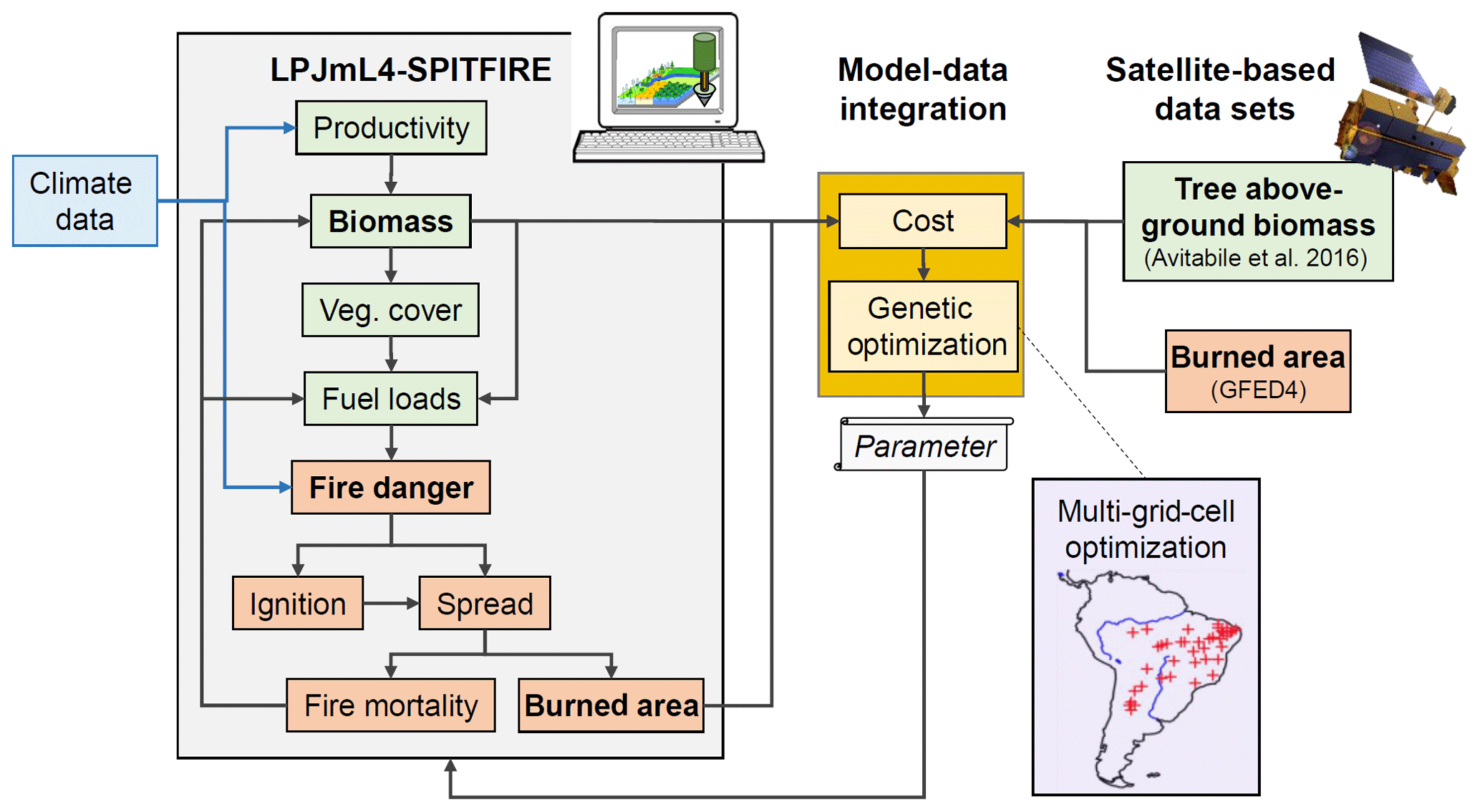
Figure 2Schematic overview of the model–data integration approach to estimate parameters of LPJmL4-SPITFIRE against satellite-based datasets of burned area and aboveground biomass
2.1 The coupled vegetation–fire model LPJmL4-SPITFIRE
2.1.1 LPJmL 4.0
The LPJmL 4.0 model (Lund-Potsdam-Jena managed Land; Schaphoff et al., 2018a, b) is a well established and validated process-based DGVM, which globally simulates the surface energy balance, water fluxes, carbon fluxes and stocks, and natural and managed vegetation from climate and soil input data. LPJmL simulates global vegetation distribution as the fractional coverage of plant functional types (PFTs), which is called foliage projective cover (FPC), and managed land as fractional coverage of crop functional types (CFTs). The establishment and survival of different PFTs is regulated through bioclimatic limits and effects of heat, productivity, and fire on plant mortality. Therefore, it enables LPJmL to investigate feedbacks, for example, between vegetation and fire. In standard settings, which are also used here, the model operates on the grid of latitude–longitude with a spinup time of 5000 years, repeating the first 30 years of the given climate dataset.
Since its original implementation by Sitch et al. (2003), LPJmL has been improved by a representation of the water balance (Gerten et al., 2004); a representation of agriculture (Bondeau et al., 2007); and new modules for fire (Thonicke et al., 2010), permafrost (Schaphoff et al., 2013), and phenology (Forkel et al., 2014).
2.1.2 SPITFIRE
SPITFIRE (SPread and InTensity of FIRE; Thonicke et al., 2010) is a process-based fire module used in various vegetation models (e.g., Lasslop et al., 2014; Yue and Unger, 2018), including LPJmL4. We describe here its main features, which are published in Thonicke et al. (2010). SPITFIRE calculates fire disturbance by simulating the ignition, the danger, the spread, and the effects of fire separately. As ignition sources SPITFIRE considers human ignition and lightning flashes. Human ignitions (nh,ig) are calculated as a function of population density:
where
PD is the human population density (individuals per square kilometer) and a(ND) (ignitions per individual per day) describes the inclination of humans to cause fire ignitions (Eqs. 3 and 4 in Thonicke et al., 2010). ph is a parameter which is set to −0.5 in Thonicke et al. (2010). This relationship assumes that human ignitions are lowest for very low population regions and for high population regions through a higher level of urbanization and landscape fragmentation. The ignition is highest for a medium-small population density. Lightning-induced ignitions are prescribed by lightning data from the OTD/LIS Gridded Climatology dataset (Christian et al., 2003), assuming that 20 % of the flashes reach the ground and 4 % of cloud-to-ground strikes can start a fire. In the study area of South America human ignitions are by far the most dominant ignition source, due to no lightning in the dry season.
Fire danger is by default computed by using the Nesterov Index, which accounts for the maximum and dew point temperatures as well as scaling factors for different PFTs on a daily time step. In the following section, we describe the calculation of the fire danger indices in detail (Sect. 2.2). Fire duration tfire (min) is calculated as a function of the fire danger index, assuming that fires burn longer under a high fire danger:
where pt is set to −11.06 in Thonicke et al. (2010). The maximum fire duration per day is 240 min.
The calculation of the forward rate of spread, ROSf,surface (m min−1), is based on the Rothermel equations (Rothermel, 1972; Pyne et al., 1996; Wilson, 1982):
where IR is the reaction intensity, ξ the propagation flux ratio, Φw a multiplier that accounts for the effect of wind, ϵ the effective heating number, Qig the heat of pre-ignition, and ρb the fuel bulk density (Eq. 9 in Thonicke et al., 2010). ρb (kg m−3) is a PFT-dependent parameter and describes the density of the fuel which is available for burning. It is weighted over the different fuel classes. Hence, a changing PFT distribution has an impact on ROSf,surface.
The simulated fire ignitions, fire danger, and fire spread are then used to calculate the burned area, fire carbon emissions, and plant mortality. Plant mortality depends on the scorch height (SH) and the probability of mortality due to crown damage Pm(CK). SH describes the height of the flame at which canopy scorching occurs. It increases with the 2∕3 power of the surface intensity Isurface:
where F is a PFT-dependent parameter. Assuming a cylindrical crown, the proportion, CK, affected by fire is calculated as
where H is the height of the average woody PFT and CL the crown length. The probability of mortality, Pm(CK), due to crown damage is then calculated by
where rCK is a PFT-dependent resistance factor between 0 and 1, and p is in the range of 3 to 4. Disturbance by fire mortality has a large impact on the vegetation dynamics, which are calculated within LPJmL. SPITFIRE further includes a surface intensity threshold (10−6, fraction burned area per grid cell), which describes the threshold of the possible area burned below which the surface intensity is set to zero and hence burned area, emissions, and fuel consumption are set to zero.
SPITFIRE considers anthropogenic effects on fire by taking into account human ignitions but does not account for fire suppression. Only wildfires occurring in natural vegetation are simulated. Fire on managed land like agriculture or pasture areas is not implemented, which has to be taken into account if simulated burned area is compared with satellite observations.
Furthermore, we introduced a small technical change in the LPJmL4 interaction with SPITFIRE compared to the original SPITFIRE implementation: in version 4.0 of LPJmL the fire litter routine calculates the leaf and litter carbon pools in a daily time step. Since the LPJmL tree allocation works at a yearly time step, this implementation leads to an incorrect LPJmL4 and SPITFIRE interaction. We now split the fire-litter routine into two parts; the first one allocates burned matter into the litter at a daily time step without recalculating the pools, and the second one calculates the leaf and root carbon pools at a yearly time step.
2.2 Fire danger indices
The fire danger index (FDI) is a key parameter within process-based fire models such as SPITFIRE. The FDI determines the probability and the intensity of a spreading fire, which impacts fire behavior.
2.2.1 Nesterov Index-based fire danger index (FDINI)
The fire danger index within SPITFIRE is based on the daily (d) calculated Nesterov Index NI(d) (Venevsky et al., 2002), which is widely used in numeric fire simulations. The NI is a cumulative function of daily maximum temperature Tmax(d) (∘C) and dew-point temperature Tdew(d) (∘C) and set to zero at a precipitation ≥ 3 mm or a temperature ≤ 4 ∘C:
The resulting fire danger index has been calculated as in Schaphoff et al. (2018a) (slightly different compared to Thonicke et al., 2010) by taking into account the NI as measure for weather conditions and a PFT-dependent scaling factor :
where n is the number of PFTs and me the moisture of extinction, which is a PFT-dependent parameter and is weighted over the litter amount. We will use the scaling factors in the parameter optimization (Sect. 2.4).
2.2.2 Vapor-pressure-deficit-based fire danger index (FDIVPD)
We implemented a new fire danger index, based on the water vapor pressure deficit (VPD). The VPD describes the difference between the saturation water vapor pressure es and the actual water vapor pressure in the air. For the parameterization of the VPD we used an approach based on Pechony and Shindell (2009):
where T is the air temperature, RH the relative humidity, and Z the Goff–Gratch equation (Goff and Gratch, 1946) to calculate the saturation vapor pressure. The flammability F at time step t for each grid cell can then be expressed as
where VD is the vegetation density, R the total precipitation (mm d−1), and cR is a constant factor (cR=2 d mm−1). Here we used the simulated FPC from LPJmL4 as a proxy for the VD. The soil is a natural buffer for drought periods and heavy rainfall events. In the Nesterov Index this was taken into account by the cumulative nature of this index. Since the VPD-based fire danger index is not cumulative, this buffering effect is taken into account by taking the monthly mean of the precipitation. In doing so we avoid unrealistic high-flammability fluctuations in time steps with isolated events of very low or very high precipitation (R).
Based on this implementation in SPITFIRE, the resulting FDI was much smaller than the original FDINI. Hence, we scaled the VPD up with a PFT-dependent scaling factor , weighted over the corresponding FPC:
for the FDIVPD was not included in Pechony and Shindell (2009) but is important in order to allow different fire responses for different tree and grass types. We will use the scaling factors in the parameter optimization (Sect. 2.4).
In comparison to the NI, the FDIVPD requires more climate variables as input as it uses relative humidity and vegetation cover as additional fire-relevant variables. Vegetation cover has a direct link to fire risk by providing the amount of available fuel for burning. According to many studies (e.g., Ray et al., 2005; Sedano and Randerson, 2014; Seager et al., 2015) the FDIVPD is a very accurate fire danger index with a high correlation with fire occurrence, while still being relatively easy to implement in a global fire model.
The general behavior of the two indices as modeled by LPJmL as a function of relative humidity and temperature is shown in Fig. 3. The Nesterov Index shows a strong but very localized maximum for high temperatures and a low humidity. Hence a spreading fire is only possible in a very small climate range (here from ca. 25 ∘C and a relative humidity less than 0.5 medium fire danger also for wetter and colder regions. The slope towards lower VPD values is also smaller compared to the Nesterov Index. Especially in regions with temperatures colder than 20 ∘C and a relative humidity less than ca. 0.6, a fire is still possible. This might increase the area in which fires can occur compared to the Nesterov Index, which could be an important improvement, enabling SPITFIRE to simulate more fire in wetter and colder regions. The calculated VPD and NI values shown in Fig. 3 are based on a LPJmL-SPITFIRE run and thus the influence of vegetation distribution on both fire danger indices.
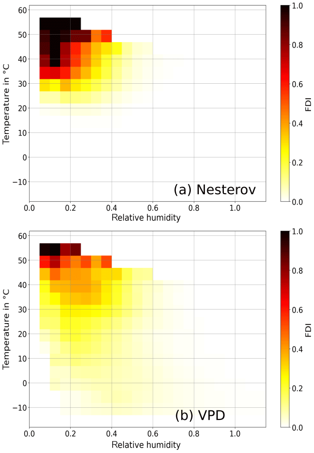
Figure 3Dependence of the simulated fire danger index on monthly mean relative humidity and temperature for (a) the Nesterov-based index and (b) the VPD-based index. Both indices were calculated with monthly data for the years 2000–2010.
2.3 Model input data
LPJmL4-SPITFIRE requires input data on daily air temperature, precipitation, longwave and shortwave downward radiation, wind, and specific humidity, which are taken from the Noah Global Land Data Assimilation System (GLDAS; Rodell et al., 2004). The data have a spatial resolution of and the time step is 3 h. We regridded and aggregated the dataset to the LPJmL resolution of and to a daily time step. We used GLDAS 2.0 for the years 1948–1999 and version GLDAS 2.1 for the years 2000–2017. GLDAS 2.1 uses multiple satellite- and ground-based observational data as well as advanced land-surface modeling and data assimilation techniques. GLDAS 2.0 is forced entirely with the Princeton meteorological forcing data (Civil and Environmental Engineering/Princeton University, 2006). Because LPJmL4 requires at least 30 years of climate data for its spinup (Sect. 2.1.1), the time span covered by GLDAS 2.1 is too short. To run the model, we used both climate datasets, but we used the years 2003–2013 from GLDAS 2.1 for the optimization and 2005–2015 for the evaluation period.
Furthermore, LPJmL4-SPITFIRE is forced with gridded constant soil texture (Nachtergaele et al., 2009) and annual information on land use from Fader et al. (2010). Atmospheric CO2 concentrations are used from Mauna Loa station (Le Quéré et al., 2015) and applied globally. The population density is taken from Goldewijk et al. (2011), and the lightning flashes are taken from the OTD/LIS satellite product (Christian et al., 2003).
2.4 Model optimization
To estimate parameters of LPJmL4-SPITFIRE, we aimed to calibrate model results against satellite observations of burned area (GFED4; Giglio et al., 2013; van der Werf et al., 2017). However, as fire occurrence and spread impact and depend on vegetation productivity, hence fuel load, we wanted to ensure to not over-fit LPJmL4 against burned area but to additionally achieve a realistic vegetation distribution. Therefore, we additionally included a satellite-derived dataset on aboveground biomass of trees (AGB; Avitabile et al., 2016) in the optimization. We combined burned area and AGB with the corresponding model outputs within a joint cost function and applied a genetic optimization algorithm to estimate model parameters (Fig. 2). The implementation of the genetic optimization algorithm (GENetic Optimization Using Derivatives (GENOUD); Mebane and Sekhon, 2011) for LPJmL is described in Forkel et al. (2014). The used cost function is based on the Kling–Gupta efficiency (KGE), which is the Euclidean distance in a three-dimensional space of model performance measures that accounts for the bias, ratio of variance, and correlation between simulations and the observations. Gupta et al. (2009) showed that the KGE that performs in an optimization setup is better than, for example, the Nash–Sutcliffe efficiency (and hence the mean square error). We extended the KGE by defining it for multiple datasets (i.e., burned area and AGB):
where and are mean values (bias component) over space (i.e., different grid cells) and time (e.g., months) of simulations s and the observations o, respectively. σs and σo are variances (variance component) and r is the Pearson correlation coefficient over space and time. The optimization was performed for 40 grid cells in South America to represent a variety of fire regimes (Fig. 2). We selected the grid cells manually to cover active fire regions (either in the model or in the evaluation data), specifically in the Cerrado and Caatinga. We selected a high density of grid cells in the Caatinga region to improve the very poor model performance in this region. To make sure that the model performance in the Caatinga and Cerrado regions was not achieved at the cost of a poor performance in other areas, we also additionally selected some cells in areas where initial fire modeling gave good results, as well as in areas where minimal or no fire occurred (central Brazilian Amazon). After inspection of the results, minor adjustments were made and the selection of the grid cells was modified to account for neglected regions (which showed worsening of the model performance). These initial analyses actually demonstrate that the choice of grid cells is important for the model optimization, and this requires the development of a more thorough selection method in future model optimization applications.
Several parameters of LPJmL4-SPITFIRE were included in the optimization that covers different fire processes (see Table 2): ignition (human ignition parameter ph, Eq. 2), fire danger (scaling factors FDI ( and ), Eqs. 10 and 13), fire spread (fire duration pt, Eq. 3), fuel bulk density (ρb, Eq. 4), surface intensity threshold, and fire effects (scorch height parameter F, Eq. 5; crown mortality parameter rCK, Eq. 7). While pt, ph, and the surface intensity threshold are global parameters (for all PFTs), the others were optimized for each PFT separately. Since we focus here on tropical South America, we used tropical broadleaved evergreen (TrBE), tropical broadleaved raingreen (TrBR), and tropical herbaceous (TrH) PFTs for the optimization.
In genetic optimization algorithms, each model parameter is called an individual with a corresponding fitness, which represents the cost of the model against the observations. At the beginning of the optimization process, the GENOUD algorithm creates a generation of individuals based on random sampling of parameter sets within the prescribed parameter ranges. After the calculation of the cost of all individuals of the first generation, a next generation is generated by cloning the best individuals, by mutating the genes or by crossing different individuals (Mebane and Sekhon, 2011). This results, after some generations, in a set of individuals with highest fitness, i.e., parameter sets with minimized cost. To find an optimum parameter set, we also used the BFGS gradient search algorithm (named after the authors: Broyden, 1970; Fletcher, 1970; Goldfarb, 1970; Shanno, 1970) within the GENOUD algorithm. An optimized parameter set of the BFGS algorithm is used as the individuals in the next generation. We were applying the GENOUD algorithm with 20 generations and a population size of 800 individuals per generation, which corresponds to 16 000 single model runs. We decided on this number of iterations because the cost kept almost constant in the last iterations and the parameter values did not change to the 6th digit, beyond which changes are not really relevant for model applications. During the optimization, we ran the model parallel for each grid cell (40 grid cells and CPUs, 3.2 GHz) and had a total optimization time of ca. 24 h.
The comparison of the two presented fire danger indices is the main objective of this study. Hence the optimization of the PFT-dependent FDI scaling factors and is crucial and obligatory for the VPD because of no prior values. Accordingly, we conducted two different optimization experiments using LPJmLmdi: first using a FDI based on the VPD (VPDoptim hereafter) and secondly using a FDI based on the NI (NIoptim hereafter). Both resulting parameter sets were then used for LPJmL4 runs and were compared to the unoptimized original model version using the NI (NIorig hereafter) and various evaluation datasets.
2.5 Evaluation data
We used burned area from the Global Fire Emissions Database (GFED4; Giglio et al., 2013; van der Werf et al., 2017), in the model optimization and to evaluate model results. The global dataset is available at a resolution of in a monthly time step from 1997 until 2016. The GFED burned area product is based on the 500 m Collection 5.1 MODIS Direct Broadcast Monthly Burned Area product (MCD64A1, after 2001). We used data for the years 2003–2013 in the optimization in order to not include potential inconsistencies between the GLDAS 2.0 and 2.1 climate datasets or between burned area observations within GFED that originate from different satellite sensors. The GFED product comes with a stratification of burned area by land cover from the MODIS land cover map at a resolution of 500 m (Giglio et al., 2013). As LPJmL does not simulate fire on managed lands, we excluded burned area on cropland classes from model–data comparisons. Due to a lack of data, however, we did not account for the proportion of pastures. To constrain the simulated vegetation distribution, we used the AGB dataset from Avitabile et al. (2016). This dataset is approximately representative for the late 2000s and therefore we compared it against simulated AGB for the years 2009–2011. We regridded all datasets to a resolution. In addition, we used maps of PFTs as derived from the ESA CCI land cover map V2.0.7 (Li et al., 2018; Forkel et al., 2014).
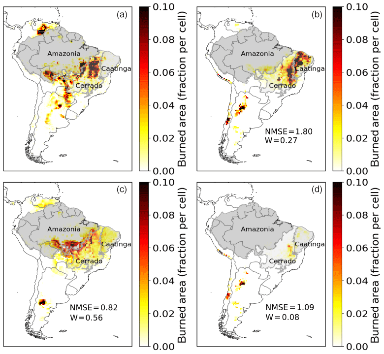
Figure 4Yearly burned area over a mean from 2005 to 2015 as fraction per cell. (a) GFED4 evaluation data of burned area excluding crops and simulated burned area by SPITFIRE using the (b) NIorig version, (c) VPDoptim version, and (d) NIoptim version.
2.6 Evaluation metrics
To quantify the performance of the model output, we applied the Pearson correlation between two time series, the normalized mean square error (NMSE; Kelley et al., 2013) and the Willmott coefficient of agreement (W; Willmott, 1982), to describe differences between the model simulation and the reference datasets. The NMSE is calculated by
where yi is the simulated and xi the observed values in the grid cell i; is the mean observed value. The NMSE is 0 for perfect agreement between simulated and modeled results, 1.0 if the model is as good as using the observed mean as a predictor, and larger than 1.0 if the model performs worse than that. We chose the NMSE to represent and compare the model errors as it has a squared error term, which puts a stronger emphasis on large deviations between simulations and observations as compared to a linear term, and due to its normalization it is comparable across different parameters. Especially for fire simulations, we have a relatively large deviation between simulations and observations.
The Willmott coefficient of agreement is given by
which additionally accounts for the area weight Ai of the grid cell i. The Willmott coefficient is a squared index, where a value of 1 stands for perfect agreement between simulated and modeled runs and gets smaller for worse agreements with a minimum of 0. Unlike the coefficient of determination, the Willmott coefficient is additionally sensitive to biases between simulations and observations.
3.1 Performance of optimized fire danger index formulations
Overall, the yearly burned area simulated by the standard SPITFIRE model (using the original Nesterov Index, NIorig) showed poor simulation results over South America as compared to the GFED4 evaluation dataset (Fig. 4a, b: NMSE = 1.80, W= 0.27). The average yearly burned area (without croplands) for South America was ca. 14×106 ha, about 25 % smaller than the observed burned area of 19×106 ha in the shown period from 2005 to 2015. The spatial pattern of the modeled burned area agreed well with the GFED4 data in the region of the Cerrado that is close to the Caatinga border, while the fires in other semiarid regions of the continent were underestimated. For example, simulated fire is underestimated in the savanna areas in the northern part of South America (on the Columbian–Venezuelan border) even though there is a strong signal visible in the satellite observations. The biomes of Caatinga and Cerrado, which are of special interest in this study, showed very different results: while fire in Caatinga was overestimated, it was underestimated in the Cerrado.
The optimized version using NIoptim (Fig. 4d) led to an overall decrease in fire, with a slight improvement in NMSE (1.09) as compared to NIorig and a worse Willmott coefficient of 0.08. Although the overestimation of fire in Caatinga was reduced, all the fires across South America also have decreased significantly, which led to a general underestimation of fire by 90 % (2×10⁶ ha). The optimized version, using VPDoptim (Fig. 4c), clearly improved the model performance, mainly by shifting much of the simulated burned area from the sparsely vegetated Caatinga towards the Cerrado region (NMSE = 0.82 and W= 0.56). In addition, by using VPDoptim, the model results also showed fire occurrence in northern South America, where fire was not at all or only minimally simulated when using NIoptim or NIorig. The total burned area was in this model version ca 20 % smaller than the evaluation dataset (16×106 ha).
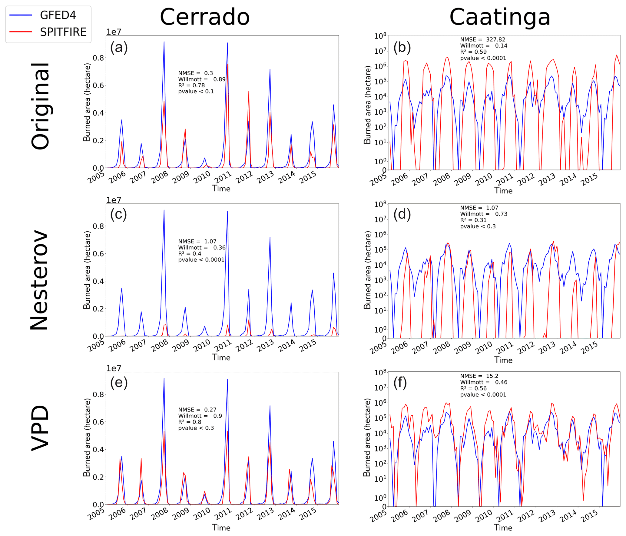
Figure 5Time series of monthly burned area from 2005 to 2015 simulated by SPITFIRE (red lines) compared to GFED4 evaluation data (blue lines) for (a) the Cerrado region using NIorig, (b) the Caatinga region using the NIorig, (c) the Cerrado region using NIoptim, (d) the Caatinga region using NIoptim, (e) the Cerrado region using VPDoptim, and (f) the Caatinga region using VPDoptim. Note the logarithmic scale for the Caatinga, which was applied in order to account for the large differences between the different model versions (for a nonlogarithmic version see Fig. A6).
The burned area time series from 2005 to 2015 provides a more detailed view on the model performance for the fire-prone Cerrado and Caatinga regions (Fig. 5). While model performance was relatively good for the Cerrado region with NIorig (NMSE = 0.3, W= 0.89, R2=0.78), the simulated burned area was strongly overestimated in the Caatinga region throughout the whole period (NMSE = 327.82, W= 0.14, R2=0.59). After the optimization of the NI, the model performance indeed improved for the Caatinga (NMSE = 1.07, W= 0.73, R2=0.31), but at the same time the performance for the Cerrado declined (NMSE = 1.07, W= 0.36, R2=0.4). On the other hand, VPDoptim showed an improved fire representation compared to the standard settings in the Cerrado (NMSE = 0.27, W= 0.9, R2=0.8) as well as in the Caatinga (NMSE = 15.2, W= 0.46, R2=0.56). Even though fire in the Caatinga was still overestimated, the NMSE decreased by a factor of 6.
Overall, the total amount of burned area in the Cerrado was for all three model versions smaller than in the evaluation dataset. Fire occurrence in the Caatinga was, on the other hand, largely overestimated by the NIorig and the VPDoptim versions. Only in the NIoptim version the burned area of the Caatinga is on the same order of magnitude as the evaluation dataset, which also led to a large underestimation in the Cerrado (Table 1 and Fig. 4). Also the Amazonia region mostly improved by using the VPDoptim version (Table 1, Fig. A3). The R2 and the Willmott coefficient improved, while the NMSE increased slightly. With the Nesterov Index, fire was strongly underestimated in the Amazon region, while the optimized VPD fixes this underestimation. The fire is only modeled (and also observed; see Fig. 4) at the edges to the Amazon, where wood density is lower and deforestation takes place. In the closed, continuous forest area towards the center of the Amazon almost no fire is observed nor modeled. The total burned area increased from 0.7×10⁶ to 4.8×10⁶ ha (for VPDoptim), which is now a bit overestimated to the observed burned area of 3.4×10⁶ ha. Using the NIoptim all error metrics as well as the total burned area decreased.
Table 1Comparison of the burned area results in terms of NMSE, the Willmott coefficient of agreement, and the sum (ha yr−1) between NIorig, VPDoptim, NIoptim, and the GFED evaluation data.
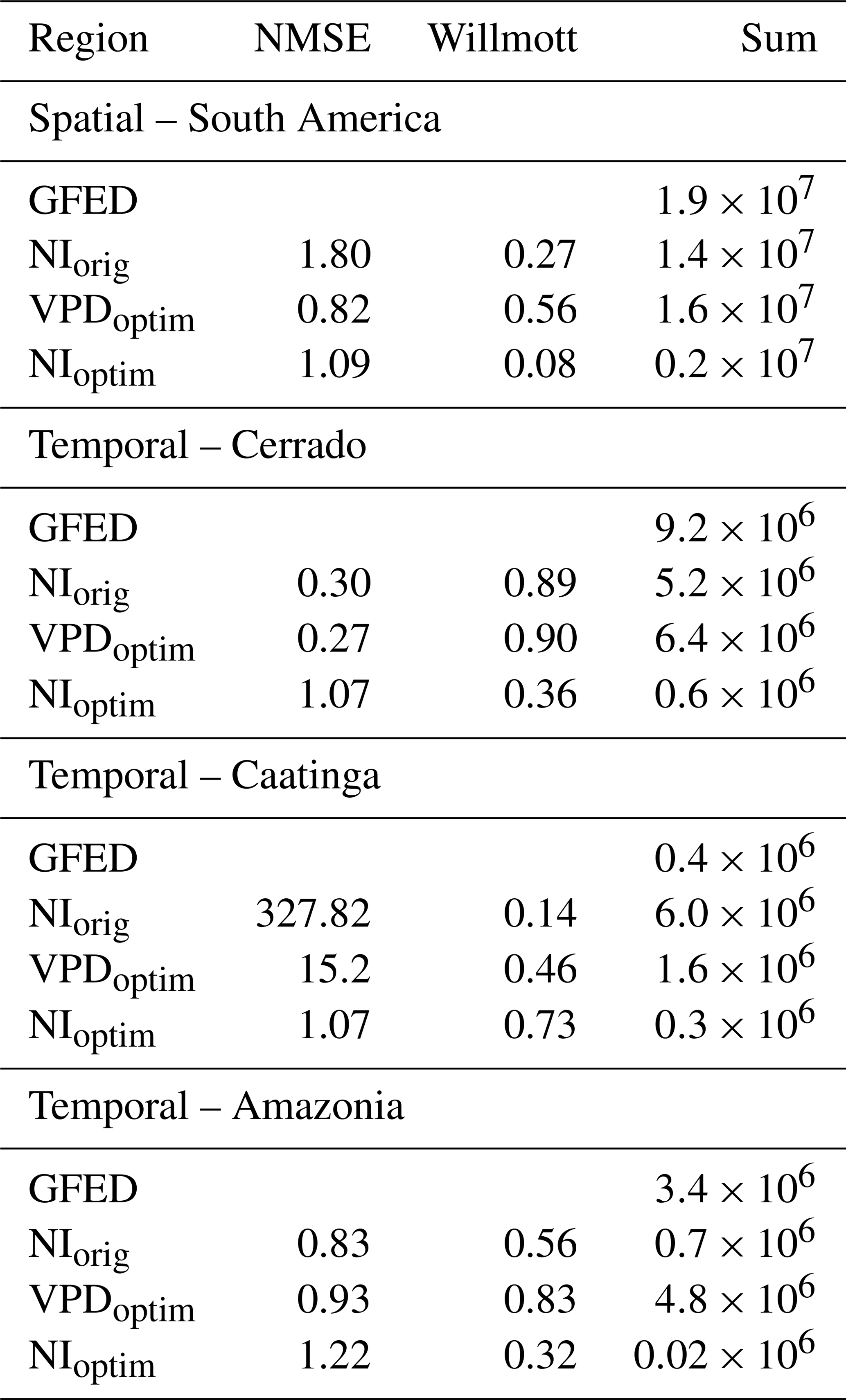
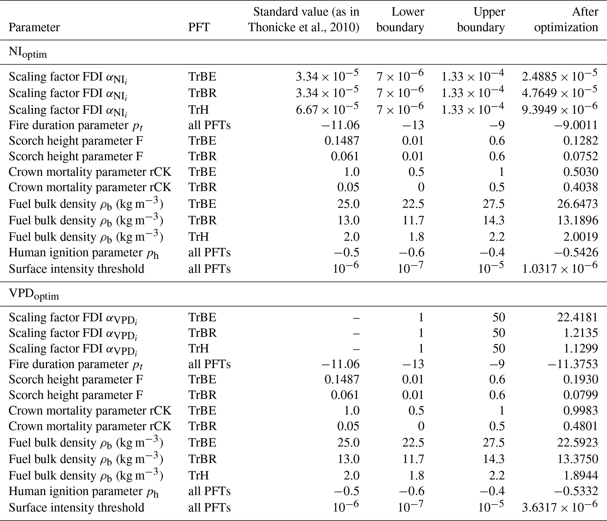
Table 2All optimized parameters with their standard values, the upper and lower boundary of the parameter ranges, and the resulting optimized value including parameters for specific PFTs and global parameter, which have the same value for all PFTs. All parameters except ρb have no unit.
3.2 Optimized model parameters
Seven fire-related parameters were optimized in order to improve the fire representation in the LPJml4-SPITFIRE model. Here we compare the optimized parameters for the different model versions in order to evaluate and discuss parameter variability and changes. Table 2 shows all parameters used for the optimization, their lower and upper boundaries, and the resulting optimized value.
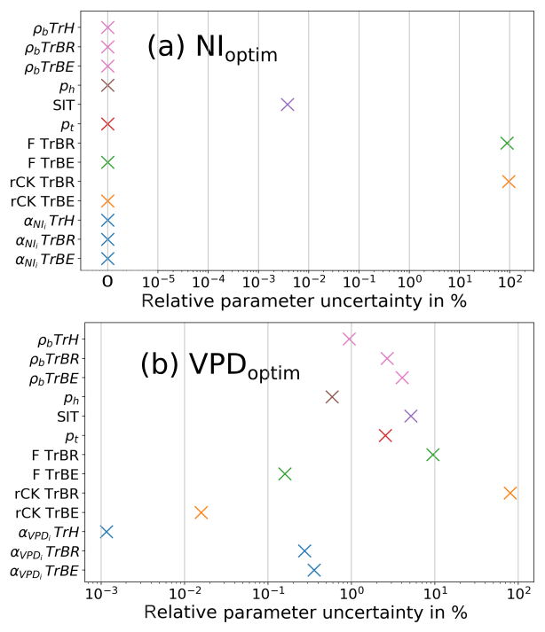
Figure 6Relative uncertainty in model parameters after optimization for (a) NIoptim and (b) VPDoptim. The relative uncertainty is the ratio of the uncertainty after the optimization (range of all parameter sets with low cost, below the 0.05 quantile) divided by the uncertainty before the optimization (range of the parameters for the optimization). Low and high values of relative uncertainty indicate strongly and weakly constrained parameters, respectively. SIT denotes the surface intensity threshold. PFT-dependent parameters are grouped with the same color.
Since the FDI directly controls the amount of modeled fire, the FDI scaling factors for the different PFTs are central for this analysis. For both optimization experiments the boundaries were, hence, set rather generously within 1 order of magnitude of the original value. In the NIoptim experiment, all scaling factors generally decreased compared to the standard values used for NIorig. Here, TrH displayed the smallest scaling factor (), followed by TrBE () and TrBR (). Since the VPD is a newly implemented fire danger index, we have no standard values to compare the optimized scaling factors with. Here, the TrBE showed the largest value (22.41), ca. 20 times as large as the TrBR (1.21) and TrH (1.13) (Table 2).
In the case of the other optimized parameters the boundaries were set smaller in order to decrease the possibility that a large error in the estimation of several parameters would lead to a better overall cost in the optimization procedure. The human ignition parameter became smaller for both optimizations, which led to a smaller amount of human ignitions (from −0.5 to −0.54 in NIoptim, and −0.53 in VPDoptim). The fuel bulk density increased for all three tropical PFTs in the NIoptim version, while for VPDoptim the fuel bulk density of the TrBE and TrH PFTs decreased and for the TrBR increased. For the NIoptim version, the fire duration parameter (pt) increased, leading to a shorter fire duration (from −11.06 to −9), while the value for the VPDoptim version stayed relatively similar (−11.37) to the prior value. The surface intensity threshold became slightly larger for the NIoptim version than the original value (from 10−6 to ). For VPDoptim the parameter increased by a factor of 3 (). The mortality-related parameters F and rCK led in the NIoptim version both to a decrease in the fire-related mortality for TrBE and an increase for TrBR PFTs. The optimized parameters for VPDoptim led to a decrease in the fire-related mortality for both PFTs except for the TrBR rCK, which led to an increased mortality.
The relative uncertainties were for most optimized parameters very small (between 0 % and 10 %), hence these parameters were strongly constrained (Fig. 6). Only the fire-mortality-related parameters (F and rCK) had large uncertainties for the TrBR and hence were weakly constrained. For VPDoptim the uncertainty in rCK (TrBR) was 0.8; for NIoptim the uncertainty in F was 0.9, and for rCK it was 1 (TrBR).
The decrease in the model error (cost) due to the optimization process was mainly due to improvement in the burned area. While for the NIoptim the cost of the burned area dataset improved by 81 %, the cost of the biomass dataset improved just by 6 %. In the case of the VPDoptim the cost of the burned area dataset improved by 49 %, whereas the biomass dataset improved by 19 % (Fig. A5).
Table 3Comparison of the results for AGB and the TrBE PFT cover in terms of NMSE and the Willmott coefficient of agreement between NIorig, VPDoptim, and NIoptim in South America (SA), in the Cerrado and in the Caatinga.
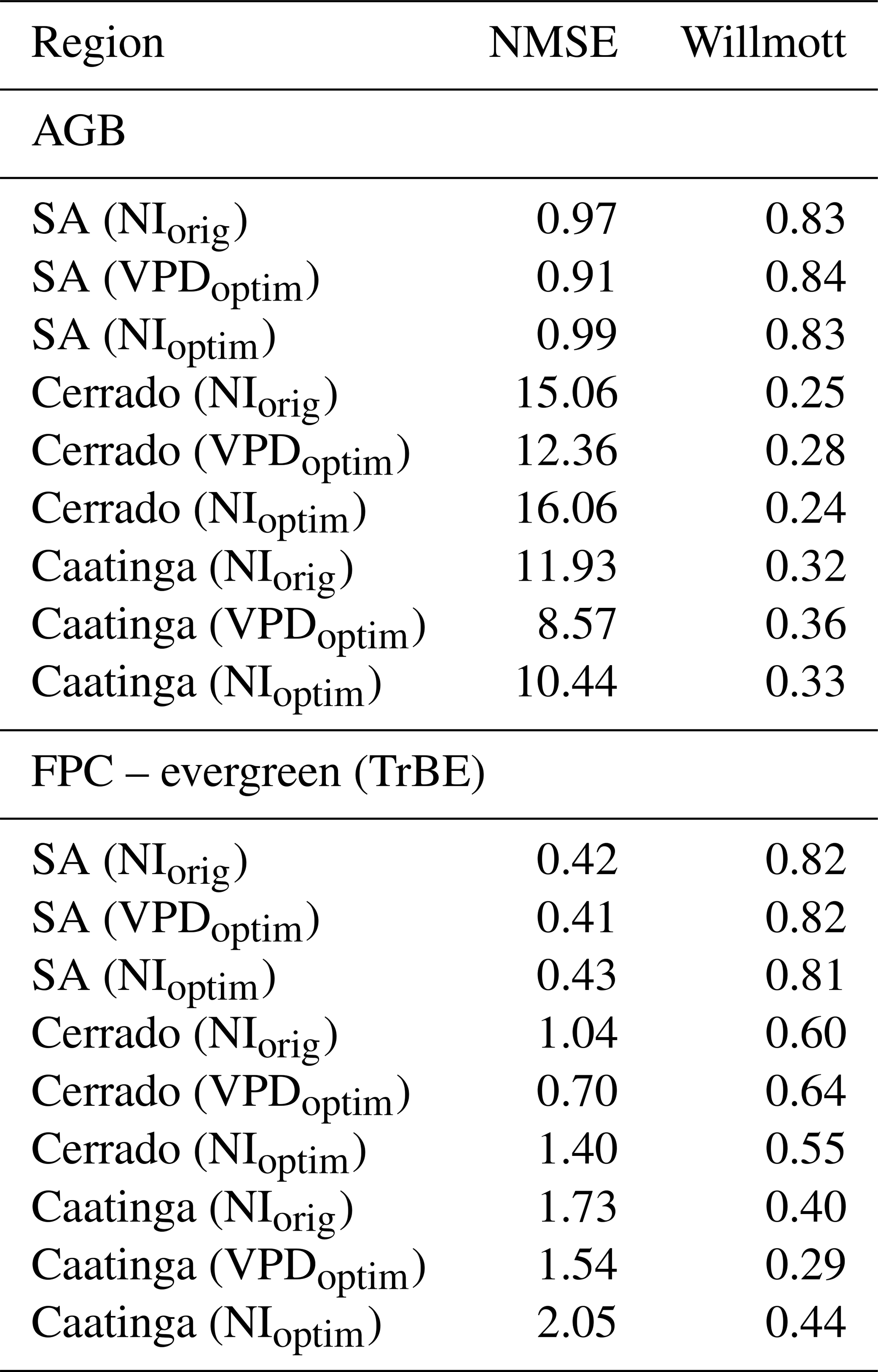
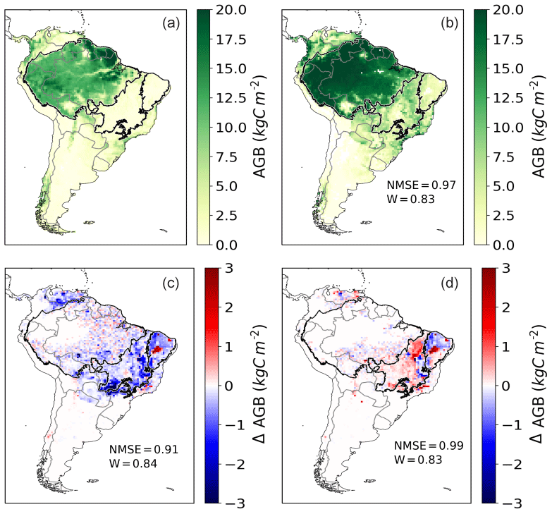
Figure 7Annual aboveground biomass (AGB) of trees over a mean from 2005 to 2015 in kg C m−2. (a) Avitabile evaluation data. (b) Simulated AGB by LPJmL4-SPITFIRE in the NIorig version. (c) Difference between VPDoptim and NIorig. (d) Difference between NIoptim and NIorig. Red (blue) color indicates a larger (smaller) biomass after the optimization.
3.3 Model evaluation for South America
The modeled aboveground biomass (AGB) of trees in South America was throughout all model versions larger than the evaluation dataset indicates (Fig. 7). Especially the biomass in the Amazon region is, with an average of ca. 20 kg C m−2, about one-third overestimated. The drier savanna regions on the continent yielded a biomass of ca. 5–10 kg C m−2, which also constitutes an overestimation in wide parts of the Cerrado and the Caatinga biomes (evaluation data show between 1 and 5 kg C m−2; see also Roitman et al., 2018).
The differences among the different model versions are marginal: the VPDoptim version had the best performance compared to the evaluation dataset (NMSE = 0.91, W= 0.84), the NIorig version had the second best performance (NMSE = 0.97, W= 0.84), and the NIoptim the worst performance (NMSE = 0.99, W= 0.83). The model optimization scheme focuses on fire parameters; hence, the model performance for AGB can only improve in areas where the fire occurrence has been modeled poorly and the vegetation–fire interactions have improved due to the optimization process. For example, in the center of the Amazon rainforest almost no fire is found in the evaluation data, nor simulated. Hence no improvement in burned area or AGB can be achieved. On the other hand, in regions where the modeling error of burned area is now reduced, this can also improve simulated AGB and hence vegetation–fire interactions. In the fire-prone Caatinga and Cerrado the VPDoptim version mostly decreased the biomass by up to 3 kg C m−2, showing a better performance compared to the evaluation dataset (e.g., in the Cerrado the NMSE decreased from 15.06 to 12.36 in the VPDoptim version compared to NIorig; see Table 3).
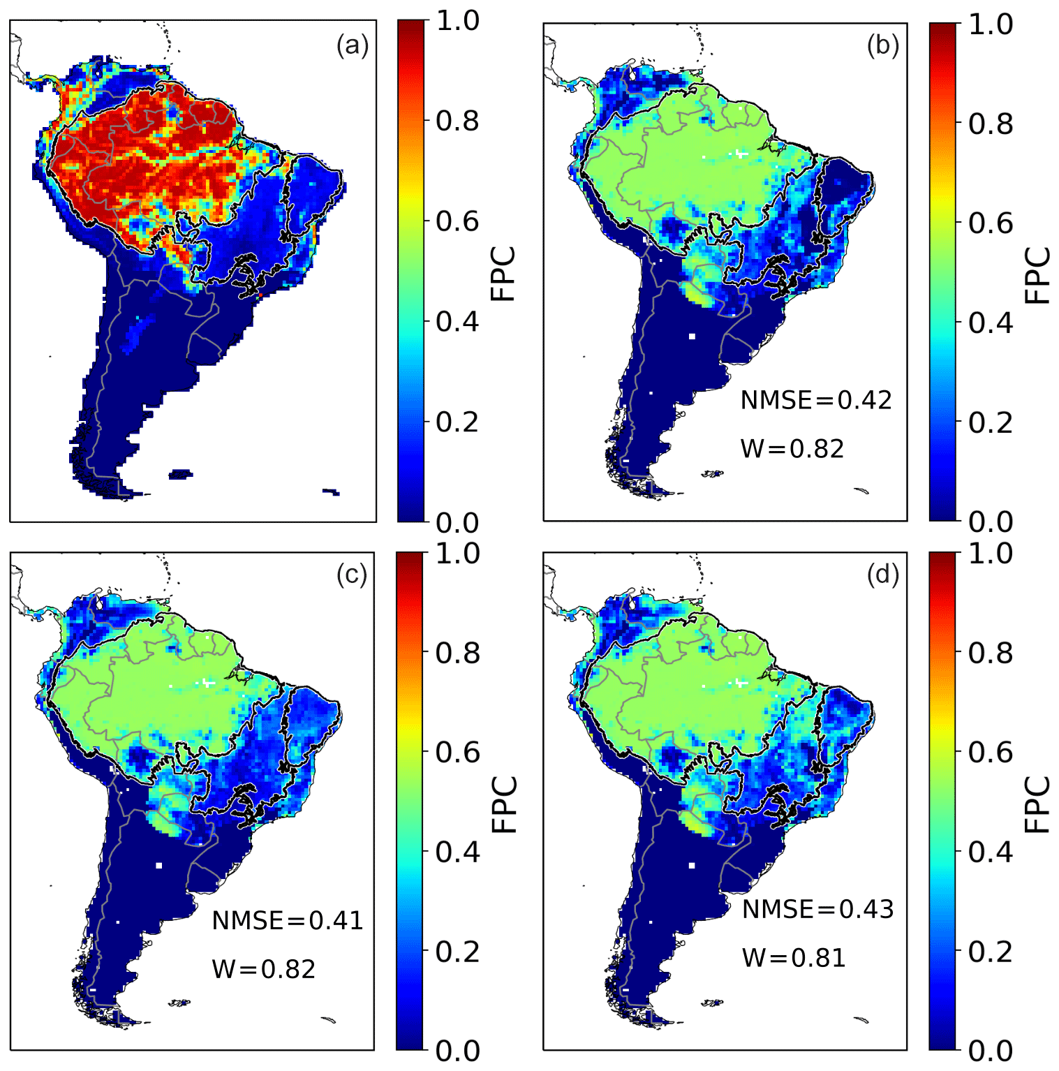
Figure 8Annual FPC cover by tropical broadleaved evergreen PFT over a mean from 2005 to 2015 as fraction per cell. (a) ESA CCI evaluation data. (b) Simulated FPC by LPJmL4-SPITFIRE using the NIorig version. (c) Simulated FPC by LPJmL4-SPITFIRE using the VPDoptim version. (d) Simulated FPC by LPJmL4-SPITFIRE using the NIoptim version.
The modeled foliage projective cover (FPC) showed for all three model versions a strong underestimation compared to the evaluation dataset of the TrBE throughout the whole Amazonian region (ca. 50 % compared to ca. 100 % in the evaluation dataset). In the fire-prone biomes of Cerrado and Caatinga, however, the TrBE PFT was sometimes overestimated (TrBE cover between 0 and 40 %, Fig. 8). In the regions with less TrBE the dominant PFT was mostly TrBR (Cerrado) or TrH (Caatinga) (see Figs. A1 and A2).
NIoptim led to an overall decrease in the model performance also in terms of the TrBE distribution, as both the NMSE and the Willmott coefficient declined compared to NIorig (NIorig: NMSE = 0.42, W= 0.82; NIoptim: NMSE = 0.43, W= 0.81).
The VPDoptim version, on the other hand, showed an slightly improved TrBE distribution (NMSE = 0.41, W= 0.82), but also in this case we obtained an even larger improvement when only the fire-prone regions of Cerrado or Caatinga are considered (Table 3). Also for the TrBR and TrH PFT distributions the optimization led to an improved performance using the VPDoptim in the Caatinga and Cerrado, whereas the PFT distribution in the Amazon remained similar to the prior PFT distribution. In the NIoptim version, parameter optimization only slightly reduced TrBR cover showing a worse performance compared to VPDoptim. However, herbaceous cover changed only slightly in all optimization experiments (Figs. A1 and A2).
In summary, our results show that the implementation of a new fire danger index based on the water vapor pressure deficit, FDIVPD, and its optimization against satellite datasets improved the simulations of fire in LPJmL4-SPITFIRE, both in terms of spatial patterns and temporal dynamics of burned area. In the following, we discuss the model improvements, limitations, and recommendations for future improvements of process-based global fire models within the DGVM framework.
4.1 Improvements in model performance
The VPD results showed a better model performance for fire in the spatial dimension, as well as in the temporal dimension (Table 1 and 3). Compared to the Nesterov Index, FDIVPD uses additional climate input such as relative humidity and precipitation. In the calculation of the Nesterov Index, precipitation is just used as a threshold. This leads to a better account of the very different climatic conditions among various biomes. Furthermore, the FDIVPD includes a direct representation of the vegetation density. The significance of this has been recently shown by findings by Forkel et al. (2019a), who have emphasized the importance of past plant productivity and fuel production for burned area. This is particularly important for differentiating between fires in biomes with similar PFT distributions. For example, the vegetation density is much larger in the Cerrado, even though the Caatinga and Cerrado have similar modeled PFT compositions, which provides more fuel and therefore leads to a higher fire danger.
While the seasonal and interannual variability in the Caatinga has improved largely using the FDIVPD (NMSE decreased by a factor of ca. 20), the improvement in the Cerrado was relatively small (NMSE decreased by ca. 10 %). This is due to the fact that the optimization tries to obtain a compromise between the different optimized cells. As the model performance was originally much better for the Cerrado, the largest improvement could be achieved for the Caatinga. We have also chosen a large number of cells in the Caatinga, because the model performance was here particularly bad. This leads to a large improvement in the time series of the Caatinga region, while the improvement for the Cerrado was less significant. With the Nesterov Index, fire was strongly underestimated in the Amazonia region, while the optimized VPD increases the modeled burned area. The fire is only present at the edges of the Amazon (both in model and observation; see Fig. 4), where tree density is lower and deforestation takes place. In the closed, continuous forest area towards the center of the Amazon almost no fire is observed and also not simulated.
Another result of the optimizing procedure, using FDIVPD, was the improvement in the PFT distribution and the aboveground biomass of trees especially in the fire-prone biomes of Caatinga and Cerrado (Fig. 8). For example, the central Amazon, where fire is a scarce event, shows almost no changes compared to the nonoptimized model version. Here, it is the improvement in the vegetation model itself, and not the fire module, which can help to improve the model performance of LPJmL4-SPITFIRE. Hence, it emphasizes that we need to include further parameters in the optimization, which impact directly the PFT distribution, biomass, and fire to obtain a significant improvement in the spatial and temporal distribution of both vegetation and fire. However, this study focused solely on the parameters within the SPITFIRE module. Due to the focus on fire-related parameters, the cost of the burned area dataset decreases much more than the cost of the biomass dataset (Fig. A5). Hence we only get a substantial improvement in model performance in semiarid fire-prone biomes, where vegetation dynamics and fire are strongly coupled. During the optimization process most of the optimized parameters were well constrained, except for the mortality-related parameters for the TrBR PFT (Fig. 6). The TrBR PFT is dominant in the fire-prone regions, where the mortality-related parameters have a large impact on vegetation dynamics. Hence, they impact multiple LPJmL routines, which are responsible for the PFT distribution and carbon cycling. This leads in turn to a less certain parameter estimation. In order to better constrain these parameters, the optimization of vegetation model parameters would be necessary to decrease the uncertainties.
The fire danger index scaling factors ( and ) convert the quantified fire risk (NI or VPD) into the actual fire danger (FDI). Both scaling factors thus set the magnitude of the fire danger for the different PFTs. Hence they impact directly the fire spread, burned area, and the number of fires and indirectly fire mortality. These very important parameters vary significantly for the different PFTs. TrH has the smallest scaling factor for both FDIs, which leads to a lower fire danger compared to the other PFTs. This indicates a prior overestimation of the fire danger of grass in tropical South America, as grasslands are generally parameterized to have a low fire resistance and moisture content and can hence burn very easily. This overestimation, compared to tree PFTs, was decreased by the optimization. In the case of the VPD, the TrBR is scaled by a much smaller factor than the TrBE, which led to a lower fire danger index. This is due to the fact that the TrBR is dominant in dry and fire-prone regions, which experience frequent fires. Here the burned area was often overestimated by SPITFIRE (e.g., Caatinga or eastern Cerrado) and is now decreased. On the other hand, a larger FDI for the TrBE allows more fire in wetter regions at the edge between the Cerrado and the Amazon rainforests, where TrBE is more dominant. The mortality risk of TrBE for VPDoptim remains close to the prior value of 1, confirming previous assumptions about its fire sensitivity; the rCK for TrBR increased to 0.48, close to the upper boundary. This means a mortality risk of 50 % when the full crown is scorched and a 7 % mortality risk when 50 % of the crown is scorched, which makes the TrBR less resistant against crown damage than before. Due to this change, the overestimation of biomass in the original model for the Cerrado and Caatinga regions decreased (see Fig. 7).
4.2 Limitations of the optimization process
Generally, optimizing a model against burned area is challenging because of (1) the skewed statistical distribution of burned area and (2) temporal or spatial mismatches in simulated burning can cause large model–data errors. These issues can be avoided with the choice of an appropriate cost function. For example, squared-error metrics tend to underestimate the variance in burned area in comparison to, for example, the Kling–Gupta efficiency, as has been shown in the optimization of an empirical model for burned area (see Table A3 in Forkel et al., 2017). Here, the optimum parameter set for the Nesterov Index-based model resulted in almost no fires across South America. Thereby, the optimization algorithm tries to decrease the model error by tending towards a conservative “no fire strategy” for all biomes. This result nicely demonstrates the need to evaluate model optimization results against spatially and temporally independent data and independent variables (Keenan et al., 2011).
The Nesterov Index is not able to capture fire variability within the Caatinga and the Cerrado at the same time. This shows that the difference in the PFT distribution between these two biomes is not adequately modeled by LPJmL or just using PFT-dependent scaling factors did not sufficiently improve the model performance when using the Nesterov Index. On the other hand, using the VPD fire danger index reduced the model error for burned area in both biomes, by improving the modeled performance for the Caatinga and maintaining the good performance of the Cerrado region. Since improved performance of the fire model mainly had a minor effect on improving FPC of the tropical PFTs, the presented optimization scheme has to go along with process-based improvements in both the fire and in the vegetation modules of LPJmL.
Fire largely depends on the vegetation type and their associated flammability, fire tolerance, and mortality. Hence an accurately modeled vegetation distribution is crucial for a good model performance in terms of burned area and fire effects (Forkel et al., 2019a; Rogers et al., 2015). As shown in Figs. 8, A1, and A2, the modeled PFT coverage showed an equal distribution of tropical raingreen and evergreen PFTs throughout wide parts of central-northern South America. Evaluation data show, however, an TrBE dominance in the wet rainforest regions and a TrBR dominance in the Cerrado and Caatinga. This emphasizes the potential to improve the fire modeling further, based on an improved PFT distribution. In the tropical rainforest the TrBR proportion is overestimated, which leads to problems in the optimization procedure, since TrBR has very different effects on fire spread and is more fire tolerant (different fuel characteristics and resulting fire intensity). This leads to a lower fire-related mortality, which fits better to the drier and fire-prone savanna-like regions (e.g., Cerrado). The poorly modeled PFT distribution also is responsible for the overestimation of the burned area in the Amazon region. Because of the too large fraction of TrBE in the Cerrado and Caatinga regions the scaling factor for this PFT is relatively high. This leads in turn to an overestimation in the Amazon region, where the fraction of the TrBE is larger.
Since the offset is very small, the years 2000–2003 (first three years of GLDAS 2.1, before the optimization period) are enough for the model to recover from the offset and the carbon pools to return to equilibrium. To exclude the possibility that long-term trends within GLDAS 2.0 changed the modeled vegetation state significantly, we tested our optimization also just based on GLDAS 2.0 data (until 2010) and on GLDAS 2.1 data (2000–2017) only, using the same years for model spinup, optimization, and evaluation. Both versions yielded similar results compared to the optimization presented in this study (results not shown).
Due to the fact that evaluation data are only available for the last 10–20 years, we are constrained to optimize the model in this relatively short time period. In South America these years were subject to an unusually large amount of severe droughts and other extreme events (Panisset et al., 2017). As a result, an optimization in this period could lead to a worse model performance in a period with less pronounced droughts. This is due to the nonlinear relationship between the drought signal in the input dataset and the resulting modeled biosphere behavior. Nonetheless, we were able to improve the interannual variability and hence the model performance to a great extent for the Caatinga and slightly for the Cerrado and Amazon regions (Figs. 5 and A3). The Cerrado already had a very good modeling performance before the optimization process, which now only slightly improved. The performance of the interannual and seasonal variability in burned area for total South America improved substantially (Fig. A3). The optimized SPITFIRE is now better able to simulate accurately the climate-dependent seasonal and interannual variability as well as the spatial extent of fire on natural land throughout the fire-prone woodlands of South America.
Systematic optimizations within a model–data integration setup of fire models which are embedded in a DGVM are still very rare. Previously, Rabin et al. (2018) optimized the fire model FINAL.1 within the land-surface model LM3. Our study differs from Rabin et al. (2018) in the conceptual design of the vegetation–fire models and the optimization process. While LM3 has been run on a 2∘ longitude by 2.5∘ latitude, this is much coarser than LPJmL with 0.5∘ by 0.5∘. This difference allows us to account for a locally better climate input, vegetation, and fire interaction. While FINAL.1 is a process-based model, many calculations (e.g., the fire spread routine) are done by multiplying the important factors and fitting the resulting values to observational data. SPITFIRE tries to model the important fire variables by simulating the underlying processes and by taking the influence of climate and the different fire ignitions into account. An advantage of FINAL.1 is the inclusion of agricultural fires based on a statistical approach. Whereas Rabin et al. (2018) used a local search algorithm (Levenberg–Marquardt algorithm) to optimize their model, we used a global search algorithm (genetic optimization). Local search algorithms depend on the chosen initial parameter sets and might eventually end up in a local optimum. A genetic optimization algorithm allows us to explore the full parameter space and hence gives a higher chance to find the global optimum. However, local search algorithms require less iterations than global search algorithms (300 in Rabin et al. (2018) vs. 16 000 in our study). Forkel et al. (2014) tested the optimization of LPJmL with different optimization algorithms and found that it was not feasible to optimize LPJmL with a local search algorithm. Rabin et al. (2018) ran the model during the optimization process only for the period of 1991–2009, whereas we made complete model runs including 5000 years of spinup in order to get a model equilibrium for each tested parameter combination.
4.3 Limitations of fire modeling in LPJmL4-SPITFIRE
In fire-prone regions the interactions between fire and vegetation dynamics are strong, hence posing a challenge for global fire models embedded in DGVMs. By just focussing on fire-related parameters, an optimization approach can only to a certain extent improve PFT distribution and simulated biomass. For a good fire representation, e.g., in the Cerrado and Caatinga, a shrub PFT could further improve the model performance. Most fires in this region occur where shrub PFTs are abundant. LPJmL tries to account for this by establishing rather small raingreen PFTs as a shrub replacement. A much better option would be a separate shrub PFT with parameters leading to a high flammability but also a low fire mortality. An optimization of LPJmL4-SPITFIRE, including shrub PFTs could yield better results than shown in this study.
Fire models embedded in DGVMs should build on a FDI which is complex enough to account for various fire dynamics, while it's parameterization should be simple enough to be accurately applied on a global scale. While the VPD is more complex and takes into account more climatic input as the Nesterov Index, it is still relatively easy to implement in a global fire model.
There are various other fire danger indices used for modeling purposes, as well as real fire danger assessment and fire forecast purposes. For example, fire-prone countries have developed their own fire danger indices (e.g., Canada, Australia), which are suited to the unique local fire regimes and vegetation dynamics. In a global modeling approach, however, we need to find one fire danger index, which suits best for all regions of the world and has a relatively easy implementation to decrease computational cost and the number of input datasets (which might be unavailable or uncertain).
Currently, SPITFIRE does not account for fire in managed land like cropland or managed grassland. We accounted for this by excluding cropland fires from the evaluated burned area dataset. We do, however, not account for the proportion of grassland, which is used for cattle ranching, for example. Since in SPITFIRE fire is not enabled on pastures, our results show a slightly smaller burned area throughout South America than could be expected with managed land included, and hence also compared to the GFED4 evaluation dataset. This effect is, however, small, because pasture lands cover a substantial fraction only in very few grid cells (e.g., southern Cerrado; Parente et al., 2017). Fire on managed land is generally difficult to predict in a DGVM, because the reason and timing of using fire depend less on climatic factors but more on social and political decisions which can vary between countries, regions, and localities. We expect further improvement in model performance especially in regions of large land-use areas with fires on pastures included (e.g., Rabin et al., 2018; Pfeiffer et al., 2013).
We significantly improved the fire representation within LPJmL4-SPITFIRE, applied for South America, by implementing a new fire danger index and applying a model–data integration setup to optimize fire-related parameters. We improved the seasonal and interannual variability, as well as the spatial pattern of burned area in South America. In addition, modeling of related vegetation variables, e.g., the biomass and the PFT distribution in the fire-prone Cerrado and Caatinga biomes have also been improved.
Optimizing fire parameters has its limits due to error propagation of the PFT distribution and hence their fire traits influencing simulated fire spread and behavior. Furthermore, it remains a challenge to find a fire danger index that is physically interpretable and can be applied globally. In this study, the parameter optimization by using FDINI led to a large underestimation of fire and a generally worse model performance when focusing on the Cerrado and Caatinga biomes. However, implementing the more complex FDIVPD, and optimizing it thereafter, led to an improved model performance compared to the original SPITFIRE implementation for South America. Our results demonstrate that an improvement in model processes, as well as a systematic model–data optimization, is required in order to obtain a more accurate fire representation within complex DGVMs, where observations or experimental evidence to constraint fire parameter are scarce. This work highlights the potential for future model–data integration approaches to obtain a better fire model performance in a global setting, based on improved vegetation dynamics within LPJmL4.
The model code of LPJmL4 is publicly available through the PIK (Potsdam Institute for Climate Impact Research) GitLab server at https://gitlab.pik-potsdam.de/lpjml/LPJmL (last access: 7 November 2019), and an exact version of the code described here is archived under https://doi.org/10.5281/zenodo.3497213 (Drüke et al., 2019). The R package for LPJmL is publicly available at https://gitlab.pik-potsdam.de/lpjml/LPJmLmdi (last access: 7 November 2019) and the exact version of the package used here is archived under https://doi.org/10.5281/zenodo.3497201 (Forkel and Drüke, 2019).
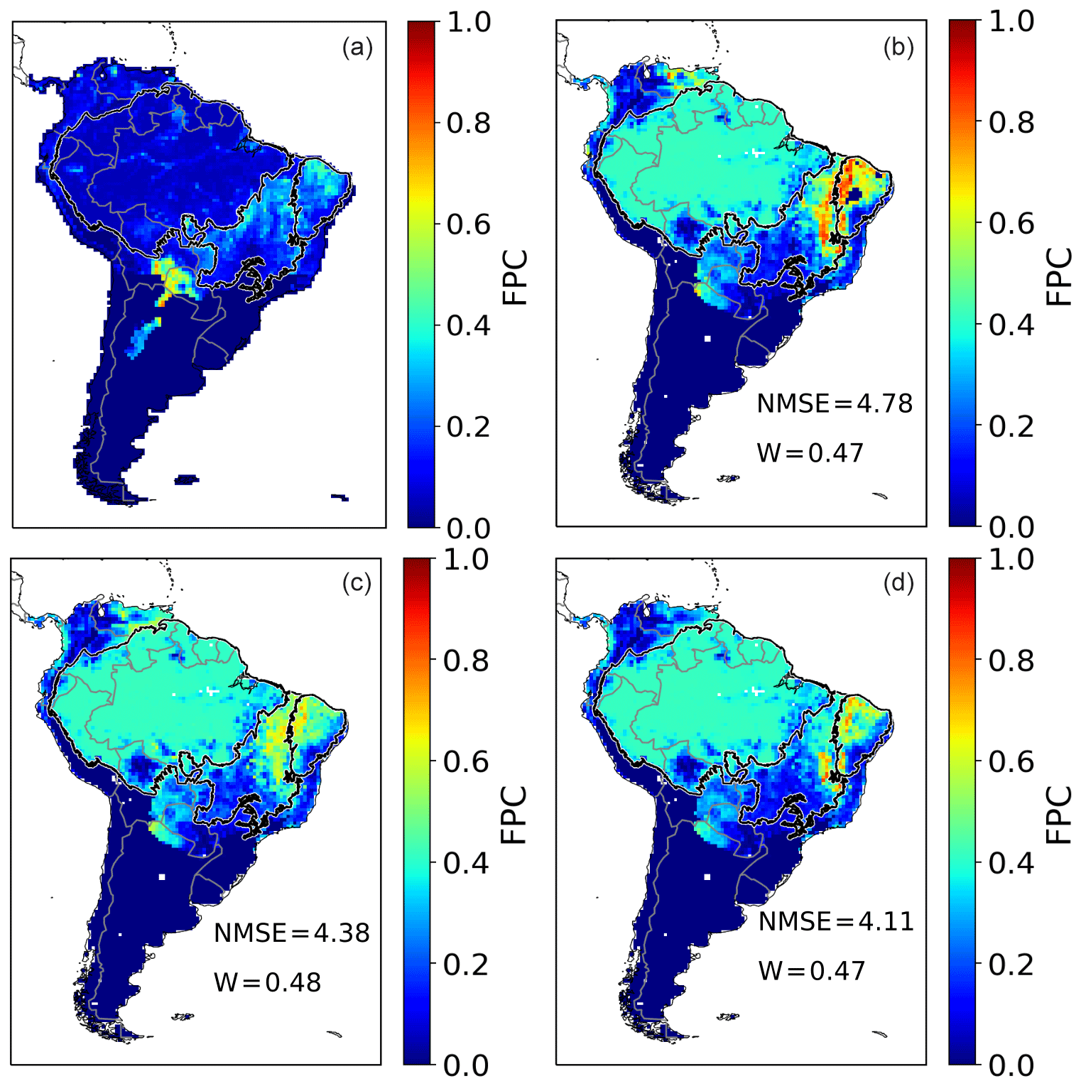
Figure A1Annual FPC cover by tropical broadleaved raingreen PFT over a mean from 2005 to 2015 as fraction per cell. (a) ESA CCI evaluation data. (b) Simulated FPC by LPJmL4-SPITFIRE using the NIorig version. (c) Simulated FPC by LPJmL4-SPITFIRE using the VPDoptim version. (d) Simulated FPC by LPJmL4-SPITFIRE using the NIoptim version.

Figure A2Annual FPC cover by tropical herbaceous PFT over a mean from 2005 to 2015 as fraction per cell. (a) ESA CCI evaluation data. (b) Simulated FPC by LPJmL4-SPITFIRE using the NIorig version. (c) Simulated FPC by LPJmL4-SPITFIRE using the VPDoptim version. (d) Simulated FPC by LPJmL4-SPITFIRE using the NIoptim version

Figure A3Time series of monthly burned area from 2005 to 2015 simulated by SPITFIRE (red lines) compared to GFED4 evaluation data (blue lines) for (a) the Amazonia region using NIorig, (b) total South America using the NIorig, (c) the Amazonia region using NIoptim, (d) total South America using NIoptim, (e) the Amazonia region using VPDoptim, and (f) total South America using VPDoptim.
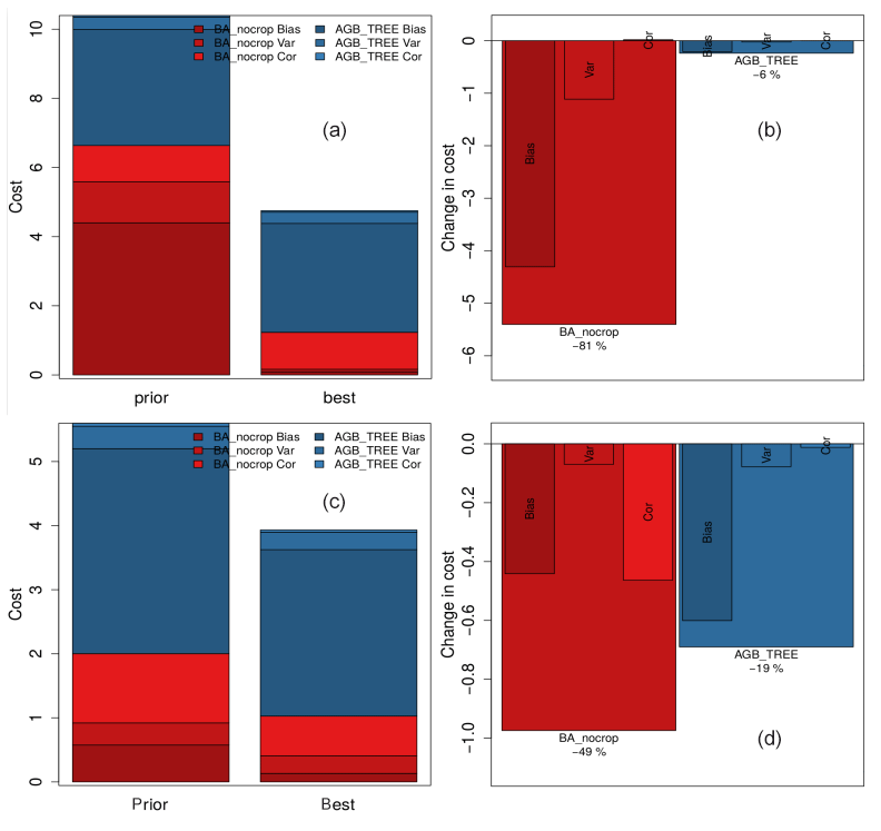
Figure A4Cost reduction of the burned area and the biomass during the optimization process by showing the various components of the cost that are related to model–data bias, variance ratio, and correlation. The cost for burned area for NIoptim decreased by ca. 81 %, whereas the cost of the biomass only decreases by ca. 6 % (a, b). For VPDoptim the cost decreased by ca. 48 % for burned area and ca. 19 % for the biomass (c, d). Hence the impact of the optimization process on burned area is much larger due to the focus on fire parameters.
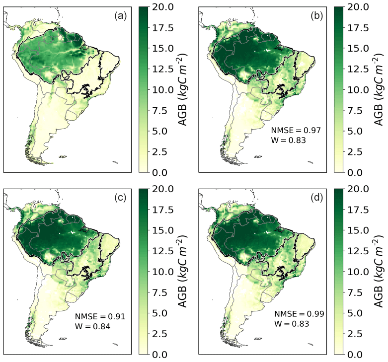
Figure A5Annual aboveground biomass (AGB) of trees over a mean from 2005 to 2015 in kg C m−2. (a) Avitabile evaluation data. (b) Simulated AGB by LPJmL4-SPITFIRE in the NIorig version. (c) Simulated AGB by LPJmL4-SPITFIRE in the VPDoptim version. (d) Simulated AGB by LPJmL4-SPITFIRE in the NIoptim version.
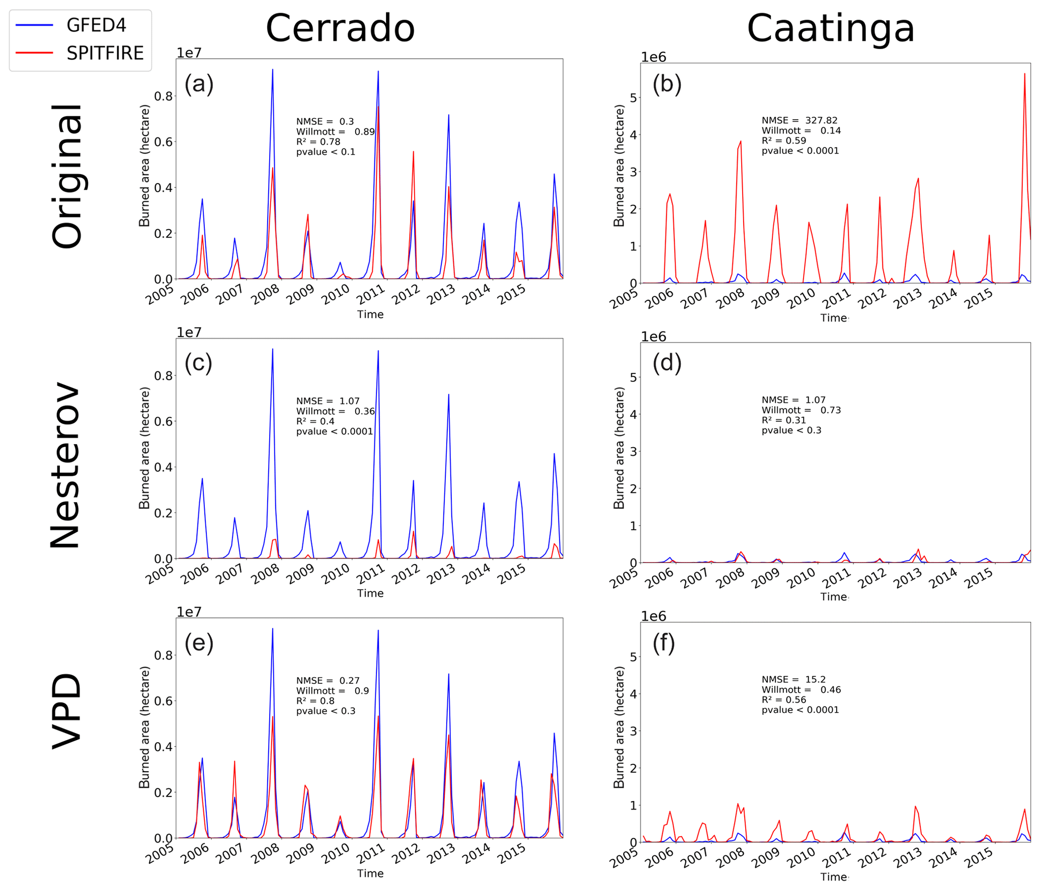
Figure A6Time series of monthly burned area from 2005 to 2015 simulated by SPITFIRE (red lines) compared to GFED4 evaluation data (blue lines) for (a) the Cerrado region using NIorig, (b) the Caatinga region using the NIorig, (c) the Cerrado region using NIoptim, (d) the Caatinga region using NIoptim, (e) the Cerrado region using VPDoptim, and (f) the Caatinga region using VPDoptim.
MD, MF, and KT designed the study in discussion with MC, MB, BS, and JK. MD and MF implemented the model–data integration framework for LPJmL4. MD and WvB implemented the new fire danger index. MD performed the analysis with inputs from MF. MD wrote the paper with inputs from all co-authors.
The authors declare that they have no conflict of interest.
This paper was developed within the scope of the IRTG 1740/TRP 2015/50122-0, funded by the DFG/FAPESP (Markus Drüke and Kirsten Thonicke). Manoel Cardoso acknowledges support from the projects FAPESP 2015/50122-0 (São Paulo Research Foundation) and CNPq 314016/2009-0 (Brazilian National Council for Scientific and Technological Development). Matthias Forkel acknowledges funding through the Technische Universität Wien Wissenschaftspreis 2015. Mercedes Bustamante acknowledges support of the Brazilian Research Network on Global Climate Change (Rede Clima) and of the National Institute of Science and Technology for Climate Change Phase 2 under CNPq, grant 465501/2014-1, FAPESP, grant 2014/50848-9, and the National Coordination for High Level Education and Training (CAPES), grant 16/2014. Kirsten Thonicke and Boris Sakschewski acknowledge funding from the BMBF- and Belmont Forum-funded project “CLIMAX: Climate Services Through Knowledge Co-Production: A Euro-South American Initiative For Strengthening Societal Adaptation Response to Extreme Events”, grant no. 01LP1610A.
This research has been supported by the IRTG 1740 (DFG/FAPESP) (grant no. TRP 2015/50122-0), the FAPESP (grant no. 2015/50122-0), the CNPq (grant no. 314016/2009-0), the CNPq (grant no. 465501/2014-1), the FAPESP (grant no. 2014/50848-9), the CAPES (grant no. 16/2014), and the BMBF and Belmont Forum (grant no. 01LP1610A).
The article processing charges for this open-access publication were covered by the Potsdam Institute for Climate Impact Research (PIK).
This paper was edited by Richard Neale and reviewed by two anonymous referees.
Alvares, C. A., Stape, J. L., Sentelhas, P. C., de Moraes Gonçalves, J. L., and Sparovek, G.: Köppen's climate classification map for Brazil, Meteorol. Z., 22, 711–728, https://doi.org/10.1127/0941-2948/2013/0507, 2013. a
Andela, N., Morton, D. C., Giglio, L., Chen, Y., van der Werf, G. R., Kasibhatla, P. S., DeFries, R. S., Collatz, G. J., Hantson, S., Kloster, S., Bachelet, D., Forrest, M., Lasslop, G., Li, F., Mangeon, S., Melton, J. R., Yue, C., and Randerson, J. T.: A human-driven decline in global burned area, Science, 356, 1356–1362, https://doi.org/10.1126/science.aal4108, 2017. a
Arpaci, A., Eastaugh, C. S., and Vacik, H.: Selecting the best performing fire weather indices for Austrian ecoregions, Theor. Appl. Climatol., 114, 393–406, https://doi.org/10.1007/s00704-013-0839-7, 2013. a, b
Avitabile, V., Herold, M., Heuvelink, G. B. M., Lewis, S. L., Phillips, O. L., Asner, G. P., Armston, J., Ashton, P. S., Banin, L., Bayol, N., Berry, N. J., Boeckx, P., de Jong, B. H. J., DeVries, B., Girardin, C. A. J., Kearsley, E., Lindsell, J. A., Lopez-Gonzalez, G., Lucas, R., Malhi, Y., Morel, A., Mitchard, E. T. A., Nagy, L., Qie, L., Quinones, M. J., Ryan, C. M., Ferry, S. J. W., Sunderland, T., Laurin, G. V., Gatti, R. C., Valentini, R., Verbeeck, H., Wijaya, A., and Willcock, S.: An integrated pan-tropical biomass map using multiple reference datasets, Global Change Biol., 22, 1406–1420, https://doi.org/10.1111/gcb.13139, 2016. a, b
Beuchle, R., Grecchi, R. C., Shimabukuro, Y. E., Seliger, R., Eva, H. D., Sano, E., and Achard, F.: Land cover changes in the Brazilian Cerrado and Caatinga biomes from 1990 to 2010 based on a systematic remote sensing sampling approach, Appl. Geogr., 58, 116–127, https://doi.org/10.1016/j.apgeog.2015.01.017, 2015. a
Bondeau, A., Smith, P. C., Zaehle, S., Schaphoff, S., Lucht, W., Cramer, W., Gerten, D., Lotze-Campen, H., Müller, C., Reichstein, M., and Smith, B.: Modelling the role of agriculture for the 20th century global terrestrial carbon balance, Global Change Biol., 13, 679–706, https://doi.org/10.1111/j.1365-2486.2006.01305.x, 2007. a
Broyden, C. G.: The Convergence of a Class of Double-rank Minimization Algorithms 1. General Considerations, IMA J. Appl. Math., 6, 76–90, https://doi.org/10.1093/imamat/6.1.76, 1970. a
Chambers, J. Q. and Artaxo, P.: Biosphere–atmosphere interactions: Deforestation size influences rainfall, Nat. Clim. Change, 7, 175–176, https://doi.org/10.1038/nclimate3238, 2017. a
Christian, H. J., Blakeslee, R. J., Boccippio, D. J., Boeck, W. L., Buechler, D. E., Driscoll, K. T., Goodman, S. J., Hall, J. M., Koshak, W. J., Mach, D. M., and Stewart, M. F.: Global frequency and distribution of lightning as observed from space by the Optical Transient Detector, J. Geophys. Res. Atmos., 108, 4005, https://doi.org/10.1029/2002JD002347, 2003. a, b
Chuvieco, E., Aguado, I., Yebra, M., Nieto, H., Salas, J., Martín, M. P., Vilar, L., Martínez, J., Martín, S., Ibarra, P., de la Riva, J., Baeza, J., Rodríguez, F., Molina, J. R., Herrera, M. A., and Zamora, R.: Development of a framework for fire risk assessment using remote sensing and geographic information system technologies, Ecol. Modell., 221, 46–58, https://doi.org/10.1016/j.ecolmodel.2008.11.017, 2010. a
Civil, O. and Environmental Engineering/Princeton University, D.: Global Meteorological Forcing Dataset for Land Surface Modeling, UCAR/NCAR – Research Data Archive, available at: https://rda.ucar.edu/datasets/ds314.0 (last access: 20 March 2019), 2006. a
Cochrane, M. A. and Laurance, W. F.: Synergisms among Fire, Land Use, and Climate Change in the Amazon, Ambio, 37, 522–527, https://doi.org/10.2307/25547943, 2008. a
Drüke, M., Forkel, M., von Bloh, W., Sakschewski, B., Cardoso, M., Bustamante, M., Kurths, J., and Thonicke, K.: LPJmL4 Model Code, V 4.0.003, Gitlab, https://doi.org/10.5281/zenodo.3497213, 2019. a
Fader, M., Rost, S., Müller, C., Bondeau, A., and Gerten, D.: Virtual water content of temperate cereals and maize: Present and potential future patterns, J. Hydrol., 384, 218–231, https://doi.org/10.1016/j.jhydrol.2009.12.011, 2010. a
Fletcher, R.: A new approach to variable metric algorithms, comjnl., 13, 317–322, https://doi.org/10.1093/comjnl/13.3.317, 1970. a
Forkel, M. and Drüke, M.: LPJmLmdi Model Code, V 1.31, Gitlab, https://doi.org/10.5281/zenodo.3497201, 2019. a
Forkel, M., Carvalhais, N., Schaphoff, S., v. Bloh, W., Migliavacca, M., Thurner, M., and Thonicke, K.: Identifying environmental controls on vegetation greenness phenology through model–data integration, Biogeosciences, 11, 7025–7050, https://doi.org/10.5194/bg-11-7025-2014, 2014. a, b, c, d, e
Forkel, M., Dorigo, W., Lasslop, G., Teubner, I., Chuvieco, E., and Thonicke, K.: A data-driven approach to identify controls on global fire activity from satellite and climate observations (SOFIA V1), Geosci. Model Dev., 10, 4443–4476, https://doi.org/10.5194/gmd-10-4443-2017, 2017. a, b
Forkel, M., Andela, N., Harrison, S. P., Lasslop, G., van Marle, M., Chuvieco, E., Dorigo, W., Forrest, M., Hantson, S., Heil, A., Li, F., Melton, J., Sitch, S., Yue, C., and Arneth, A.: Emergent relationships with respect to burned area in global satellite observations and fire-enabled vegetation models, Biogeosciences, 16, 57–76, https://doi.org/10.5194/bg-16-57-2019, 2019a. a, b, c
Forkel, M., Dorigo, W., Lasslop, G., Chuvieco, E., Hantson, S., Heil, A., Teubner, I., Thonicke, K., and Harrison, S. P.: Recent global and regional trends in burned area and their compensating environmental controls, Environ. Res. Commun., 1, 051005, https://doi.org/10.1088/2515-7620/ab25d2, 2019b. a
Gerten, D., Schaphoff, S., Haberlandt, U., Lucht, W., and Sitch, S.: Terrestrial vegetation and water balance–hydrological evaluation of a dynamic global vegetation model, J. Hydrol., 286, 249–270, https://doi.org/10.1016/j.jhydrol.2003.09.029, 2004. a
Giglio, L., Randerson, J. T., and van der Werf, G. R.: Analysis of daily, monthly, and annual burned area using the fourth-generation global fire emissions database (GFED4), J. Geophys. Res.-Biogeo., 118, 317–328, https://doi.org/10.1002/jgrg.20042, 2013. a, b, c, d, e
Goff, J. and Gratch, S.: List 1947, Smithsonian meteorological tables, Transactions of the American Society of Ventilation Engineering, vol. 52, p. 95, 1946. a
Goldewijk, K. K., Beusen, A., van Drecht, G., and de Vos, M.: The HYDE 3.1 spatially explicit database of human-induced global land-use change over the past 12,000 years, Global Ecol. Biogeogr., 20, 73–86, https://doi.org/10.1111/j.1466-8238.2010.00587.x, 2011. a
Goldfarb, D.: A family of variable-metric methods derived by variational means, Math. Comput., 24, 23–26, https://doi.org/10.1090/S0025-5718-1970-0258249-6, 1970. a
Gupta, H. V., Kling, H., Yilmaz, K. K., and Martinez, G. F.: Decomposition of the mean squared error and NSE performance criteria: Implications for improving hydrological modelling, J. Hydrol., 377, 80–91, https://doi.org/10.1016/j.jhydrol.2009.08.003, 2009. a
Hantson, S., Arneth, A., Harrison, S. P., Kelley, D. I., Prentice, I. C., Rabin, S. S., Archibald, S., Mouillot, F., Arnold, S. R., Artaxo, P., Bachelet, D., Ciais, P., Forrest, M., Friedlingstein, P., Hickler, T., Kaplan, J. O., Kloster, S., Knorr, W., Lasslop, G., Li, F., Mangeon, S., Melton, J. R., Meyn, A., Sitch, S., Spessa, A., van der Werf, G. R., Voulgarakis, A., and Yue, C.: The status and challenge of global fire modelling, Biogeosciences, 13, 3359–3375, https://doi.org/10.5194/bg-13-3359-2016, 2016. a, b
Harvard: Harvard WorldMap, available at: http://worldmap.harvard.edu, last access: 27 March, 2019. a
Hoffmann, W. A., Jackson, R. B., Hoffmann, W. A., and Jackson, R. B.: Vegetation–Climate Feedbacks in the Conversion of Tropical Savanna to Grassland, J. Climate, 13, 1593–1602, https://doi.org/10.1175/1520-0442(2000)013<1593:VCFITC>2.0.CO;2, 2000. a
IBGE: Mapa de Biomas e de Vegetação, available at: https://ww2.ibge.gov.br/home/presidencia/noticias/21052004biomashtml.shtm, last access: 14 February, 2019. a
Jolly, W. M., Cochrane, M. A., Freeborn, P. H., Holden, Z. A., Brown, T. J., Williamson, G. J., and Bowman, D. M. J. S.: Climate-induced variations in global wildfire danger from 1979 to 2013, Nat. Commun., 6, 7537, https://doi.org/10.1038/ncomms8537, 2015. a, b
Keeley, J. E., Pausas, J. G., Rundel, P. W., Bond, W. J., and Bradstock, R. A.: Fire as an evolutionary pressure shaping plant traits, Trends Plant Sci., 16, 406–411, https://doi.org/10.1016/j.tplants.2011.04.002, 2011. a
Keenan, T. F., Carbone, M. S., Reichstein, M., and Richardson, A. D.: The model–data fusion pitfall: assuming certainty in an uncertain world, Oecologia, 167, 587, https://doi.org/10.1007/s00442-011-2106-x, 2011. a
Keetch, J. J. and Byram, G. M.: A Drought Index for Forest Fire Control, Southeastern Forest Experiment Station, U.S. Department of Agriculture, Asheville, NC, USA, Forest Service, Res. Pap. SE-38, 35 pp., available at: https://www.fs.usda.gov/treesearch/pubs/40 (last access: 20 March 2019), 1968. a
Kelley, D. I., Prentice, I. C., Harrison, S. P., Wang, H., Simard, M., Fisher, J. B., and Willis, K. O.: A comprehensive benchmarking system for evaluating global vegetation models, Biogeosciences, 10, 3313–3340, https://doi.org/10.5194/bg-10-3313-2013, 2013. a
Knorr, W., Arneth, A., and Jiang, L.: Demographic controls of future global fire risk, Nat. Clim. Change, 6, 781–758, https://doi.org/10.1038/nclimate2999, 2016. a
Krawchuk, M. A. and Moritz, M. A.: Constraints on global fire activity vary across a resource gradient, Ecology, 92, 121–132, https://doi.org/10.1890/09-1843.1, 2011. a
Lahsen, M., Bustamante, M. M. C., and Dalla-Nora, E. L.: Undervaluing and Overexploiting the Brazilian Cerrado at Our Peril, Environment, 58, 4–15, https://doi.org/10.1080/00139157.2016.1229537, 2016. a, b
Langmann, B., Duncan, B., Textor, C., Trentmann, J., and van der Werf, G. R.: Vegetation fire emissions and their impact on air pollution and climate, Atmos. Environ., 43, 107–116, https://doi.org/10.1016/j.atmosenv.2008.09.047, 2009. a
Lasslop, G., Thonicke, K., and Kloster, S.: SPITFIRE within the MPI Earth system model: Model development and evaluation, J. Adv. Model. Earth Syst., 6, 740–755, https://doi.org/10.1002/2013MS000284, 2014. a
Lasslop, G., Hantson, S., and Kloster, S.: Influence of wind speed on the global variability of burned fraction: a global fire model's perspective, Int. J. Wildland Fire, 24, 989–1000, https://doi.org/10.1071/WF15052, 2015. a
Lasslop, G., Brovkin, V., Reick, C. H., Bathiany, S., and Kloster, S.: Multiple stable states of tree cover in a global land surface model due to a fire-vegetation feedback, Geophys. Res. Lett., 43, 6324–6331, https://doi.org/10.1002/2016GL069365, 2016. a
Le Quéré, C., Moriarty, R., Andrew, R. M., Canadell, J. G., Sitch, S., Korsbakken, J. I., Friedlingstein, P., Peters, G. P., Andres, R. J., Boden, T. A., Houghton, R. A., House, J. I., Keeling, R. F., Tans, P., Arneth, A., Bakker, D. C. E., Barbero, L., Bopp, L., Chang, J., Chevallier, F., Chini, L. P., Ciais, P., Fader, M., Feely, R. A., Gkritzalis, T., Harris, I., Hauck, J., Ilyina, T., Jain, A. K., Kato, E., Kitidis, V., Klein Goldewijk, K., Koven, C., Landschützer, P., Lauvset, S. K., Lefèvre, N., Lenton, A., Lima, I. D., Metzl, N., Millero, F., Munro, D. R., Murata, A., Nabel, J. E. M. S., Nakaoka, S., Nojiri, Y., O'Brien, K., Olsen, A., Ono, T., Pérez, F. F., Pfeil, B., Pierrot, D., Poulter, B., Rehder, G., Rödenbeck, C., Saito, S., Schuster, U., Schwinger, J., Séférian, R., Steinhoff, T., Stocker, B. D., Sutton, A. J., Takahashi, T., Tilbrook, B., van der Laan-Luijkx, I. T., van der Werf, G. R., van Heuven, S., Vandemark, D., Viovy, N., Wiltshire, A., Zaehle, S., and Zeng, N.: Global Carbon Budget 2015, Earth Syst. Sci. Data, 7, 349–396, https://doi.org/10.5194/essd-7-349-2015, 2015. a
Li, W., MacBean, N., Ciais, P., Defourny, P., Lamarche, C., Bontemps, S., Houghton, R. A., and Peng, S.: Gross and net land cover changes in the main plant functional types derived from the annual ESA CCI land cover maps (1992–2015), Earth Syst. Sci. Data, 10, 219–234, https://doi.org/10.5194/essd-10-219-2018, 2018. a
Mebane, Jr., W. R. and Sekhon, J. S.: Genetic Optimization Using Derivatives: The rgenoud Package for R, J. Stat. Softw., 42, 1–26, https://doi.org/10.18637/jss.v042.i11, 2011. a
Moreira de Araújo, F., Ferreira, L. G., and Arantes, A. E.: Distribution Patterns of Burned Areas in the Brazilian Biomes: An Analysis Based on Satellite Data for the 2002–2010 Period, Remote Sens., 4, 1929–1946, https://doi.org/10.3390/rs4071929, 2012. a
Nachtergaele, F. O., van Velthuizen, H. T., and Verelst, L.: Harmonized World Soil Database, available at: http://pure.iiasa.ac.at/id/eprint/8958 (last access: 4 October 2018), 2009. a
Panisset, J. S., Libonati, R., Gouveia, C. M. P., Machado-Silva, F., França, D. A., França, J. R. A., and Peres, L. F.: Contrasting patterns of the extreme drought episodes of 2005, 2010 and 2015 in the Amazon Basin, Int. J. Climatol., 38, 1096–1104, https://doi.org/10.1002/joc.5224, 2017. a
Parente, L., Ferreira, L., Faria, A., Nogueira, S., Araújo, F., Teixeira, L., and Hagen, S.: Monitoring the brazilian pasturelands: A new mapping approach based on the landsat 8 spectral and temporal domains, Int. J. Appl. Earth Obs. Geoinf., 62, 135–143, https://doi.org/10.1016/j.jag.2017.06.003, 2017. a
Pechony, O. and Shindell, D. T.: Fire parameterization on a global scale, J. Geophys. Res.-Atmos., 114, D16115, https://doi.org/10.1029/2009JD011927, 2009. a, b, c, d
Pfeiffer, M., Spessa, A., and Kaplan, J. O.: A model for global biomass burning in preindustrial time: LPJ-LMfire (v1.0), Geosci. Model Dev., 6, 643–685, https://doi.org/10.5194/gmd-6-643-2013, 2013. a
Prado, D. E.: As caatingas da América do Sul, Ecologia e conservação da Caatinga, 2, 3–74, 2003. a
Pyne, S. J., Andrews, P. L., and Laven, R. D.: Introduction to wildland fire, 2nd edn., DigitalCommons@USU, available at: https://digitalcommons.usu.edu/barkbeetles/135 (last access: 20 March 2019), 1996. a
Rabin, S. S., Ward, D. S., Malyshev, S. L., Magi, B. I., Shevliakova, E., and Pacala, S. W.: A fire model with distinct crop, pasture, and non-agricultural burning: use of new data and a model-fitting algorithm for FINAL.1, Geosci. Model Dev., 11, 815–842, https://doi.org/10.5194/gmd-11-815-2018, 2018. a, b, c, d, e, f
Ray, D., Nepstad, D., and Moutinho, P.: Micrometeorological and canopy controls of fire susceptibility in a forested amazon landscape, Ecol. Appl., 15, 1664–1678, https://doi.org/10.1890/05-0404, 2005. a, b
Rodell, M., Houser, P. R., Jambor, U., Gottschalck, J., Mitchell, K., Meng, C.-J., Arsenault, K., Cosgrove, B., Radakovich, J., Bosilovich, M., Entin, J. K., Walker, J. P., Lohmann, D., Toll, D., Rodell, M., Houser, P. R., Jambor, U., Gottschalck, J., Mitchell, K., Meng, C.-J., Arsenault, K., Cosgrove, B., Radakovich, J., Bosilovich, M., Entin, J. K., Walker, J. P., Lohmann, D., and Toll, D.: The Global Land Data Assimilation System, B. Am. Meteorol. Soc., 85, 381–394, https://doi.org/10.1175/BAMS-85-3-381, 2004. a
Rogers, B. M., Soja, A. J., Goulden, M. L., and Randerson, J. T.: Influence of tree species on continental differences in boreal fires and climate feedbacks, Nat. Geosci., 8, 228–234, https://doi.org/10.1038/ngeo2352, 2015. a
Roitman, I., Bustamante, M. M. C., Haidar, R. F., Shimbo, J. Z., Abdala, G. C., Eiten, G., Fagg, C. W., Felfili, M. C., Felfili, J. M., Jacobson, T. K. B., Lindoso, G. S., Keller, M., Lenza, E., Miranda, S. C., Pinto, J. R. R., Rodrigues, A. A., Delitti, W. B. C., Roitman, P., and Sampaio, J. M.: Optimizing biomass estimates of savanna woodland at different spatial scales in the Brazilian Cerrado: Re-evaluating allometric equations and environmental influences, PLoS One, 13, e0196742, https://doi.org/10.1371/journal.pone.0196742, 2018. a
Rothermel, R. C.: A mathematical model for predicting fire spread in wildland fuels, DigitalCommons@USU, Res. Pap. INT-115, 1, available at: https://digitalcommons.usu.edu/barkbeetles/438 (last access: 20 March 2019), 1972. a
Schaphoff, S., Heyder, U., Ostberg, S., Gerten, D., Heinke, J., and Lucht, W.: Contribution of permafrost soils to the global carbon budget, Environ. Res. Lett., 8, 014026, https://doi.org/10.1088/1748-9326/8/1/014026, 2013. a
Schaphoff, S., von Bloh, W., Rammig, A., Thonicke, K., Biemans, H., Forkel, M., Gerten, D., Heinke, J., Jägermeyr, J., Knauer, J., Langerwisch, F., Lucht, W., Müller, C., Rolinski, S., and Waha, K.: LPJmL4 – a dynamic global vegetation model with managed land – Part 1: Model description, Geosci. Model Dev., 11, 1343–1375, https://doi.org/10.5194/gmd-11-1343-2018, 2018a. a, b
Schaphoff, S., Forkel, M., Müller, C., Knauer, J., von Bloh, W., Gerten, D., Jägermeyr, J., Lucht, W., Rammig, A., Thonicke, K., and Waha, K.: LPJmL4 – a dynamic global vegetation model with managed land – Part 2: Model evaluation, Geosci. Model Dev., 11, 1377–1403, https://doi.org/10.5194/gmd-11-1377-2018, 2018b. a
Seager, R., Hooks, A., Williams, A. P., Cook, B., Nakamura, J., Henderson, N., Seager, R., Hooks, A., Williams, A. P., Cook, B., Nakamura, J., and Henderson, N.: Climatology, Variability, and Trends in the U.S. Vapor Pressure Deficit, an Important Fire-Related Meteorological Quantity, available at: https://journals.ametsoc.org/doi/abs/10.1175/JAMC-D-14-0321.1 (last access: 19 October 2018), 2015. a
Sedano, F. and Randerson, J. T.: Multi-scale influence of vapor pressure deficit on fire ignition and spread in boreal forest ecosystems, Biogeosciences, 11, 3739–3755, https://doi.org/10.5194/bg-11-3739-2014, 2014. a
Shanno, D. F.: Conditioning of quasi-Newton methods for function minimization, Math. Comput., 24, 647–656, https://doi.org/10.1090/S0025-5718-1970-0274029-X, 1970. a
Silverio, D. V., Brando, P. M., Balch, J. K., Putz, F. E., Nepstad, D. C., Oliveira-Santos, C., and Bustamante, M. M. C.: Testing the Amazon savannization hypothesis: fire effects on invasion of a neotropical forest by native cerrado and exotic pasture grasses, Philos. T. R. Soc. B, 368, 1619, https://doi.org/10.1098/rstb.2012.0427, 2013. a
Sitch, S., Smith, B., Prentice, I. C., Arneth, A., Bondeau, A., Cramer, W., Kaplan, J. O., Levis, S., Lucht, W., Sykes, M. T., Thonicke, K., and Venevsky, S.: Evaluation of ecosystem dynamics, plant geography and terrestrial carbon cycling in the LPJ dynamic global vegetation model, Global Change Biol., 9, 161–185, https://doi.org/10.1046/j.1365-2486.2003.00569.x, 2003. a
Thonicke, K., Venevsky, S., Sitch, S., and Cramer, W.: The role of fire disturbance for global vegetation dynamics: coupling fire into a Dynamic Global Vegetation Model, Global Ecol. Biogeogr., 10, 661–677, https://doi.org/10.1046/j.1466-822X.2001.00175.x, 2001. a
Thonicke, K., Spessa, A., Prentice, I. C., Harrison, S. P., Dong, L., and Carmona-Moreno, C.: The influence of vegetation, fire spread and fire behaviour on biomass burning and trace gas emissions: results from a process-based model, Biogeosciences, 7, 1991–2011, https://doi.org/10.5194/bg-7-1991-2010, 2010. a, b, c, d, e, f, g, h, i, j, k, l
van der Werf, G. R., Dempewolf, J., Trigg, S. N., Randerson, J. T., Kasibhatla, P. S., Giglio, L., Murdiyarso, D., Peters, W., Morton, D. C., Collatz, G. J., Dolman, A. J., and DeFries, R. S.: Climate regulation of fire emissions and deforestation in equatorial Asia, P. Natl. Acad. Sci. USA, 105, 20350–20355, https://doi.org/10.1073/pnas.0803375105, 2008. a
van der Werf, G. R., Randerson, J. T., Giglio, L., Collatz, G. J., Mu, M., Kasibhatla, P. S., Morton, D. C., DeFries, R. S., Jin, Y., and van Leeuwen, T. T.: Global fire emissions and the contribution of deforestation, savanna, forest, agricultural, and peat fires (1997–2009), Atmos. Chem. Phys., 10, 11707–11735, https://doi.org/10.5194/acp-10-11707-2010, 2010. a
van der Werf, G. R., Randerson, J. T., Giglio, L., van Leeuwen, T. T., Chen, Y., Rogers, B. M., Mu, M., van Marle, M. J. E., Morton, D. C., Collatz, G. J., Yokelson, R. J., and Kasibhatla, P. S.: Global fire emissions estimates during 1997–2016, Earth Syst. Sci. Data, 9, 697–720, https://doi.org/10.5194/essd-9-697-2017, 2017. a, b, c
Venevsky, S., Thonicke, K., Sitch, S., and Cramer, W.: Simulating fire regimes in human-dominated ecosystems: Iberian Peninsula case study, Global Change Biol., 8, 984–998, https://doi.org/10.1046/j.1365-2486.2002.00528.x, 2002. a, b, c, d, e
Wagner, C. E. V., Forest, P., Station, E., Ontario, C. R., Francais, R. U. E., and Davis, H. J.: Development and Structure of the Canadian Forest FireWeather Index System, Can. For. Serv., Forestry Tech. Rep, 1987. a
Willmott, C. J.: Some Comments on the Evaluation of Model Performance, B. Am. Meteorol. Soc., 63, 1309–1313, https://doi.org/10.1175/1520-0477(1982)063<1309:SCOTEO>2.0.CO;2, 1982. a
Wilson, R. A.: A reexamination of fire spread in free-burning porous fuel beds, U.S. Dept. of Agriculture, Forest Service, Intermountain Forest and Range Experiment Station, available at: http://www.sidalc.net/cgi-bin/wxis.exe/?IsisScript=COLPOS.xis&method\={p}ost&formato=2&cantidad=1&expresion=mfn=001388, (last access: 4 October 2018), 1982. a
Yue, X. and Unger, N.: Fire air pollution reduces global terrestrial productivity, Nat. Commun., 9, 5413, https://doi.org/10.1038/s41467-018-07921-4, 2018. a, b