the Creative Commons Attribution 4.0 License.
the Creative Commons Attribution 4.0 License.
 | 07 Nov 2019
GlobSim (v1.0): deriving meteorological time series for point locations from multiple global reanalyses
Xiaojing Quan
Nicholas Brown
Emilie Stewart-Jones
Stephan Gruber
Simulations of land-surface processes and phenomena often require driving time series of meteorological variables. Corresponding observations, however, are unavailable in most locations, even more so, when considering the duration, continuity and data quality required. Atmospheric reanalyses provide global coverage of relevant meteorological variables, but their use is largely restricted to grid-based studies. This is because technical challenges limit the ease with which reanalysis data can be applied to models at the site scale. We present the software toolkit GlobSim, which automates the downloading, interpolation and scaling of different reanalyses – currently ERA5, ERA-Interim, JRA-55 and MERRA-2 – to produce meteorological time series for user-defined point locations. The resulting data have consistent structure and units to efficiently support ensemble simulation. The utility of GlobSim is demonstrated using an application in permafrost research. We perform ensemble simulations of ground-surface temperature for 10 terrain types in a remote tundra area in northern Canada and compare the results with observations. Simulation results reproduced seasonal cycles and variation between terrain types well, demonstrating that GlobSim can support efficient land-surface simulations. Ensemble means often yielded better accuracy than individual simulations and ensemble ranges additionally provide indications of uncertainty arising from uncertain input. By improving the usability of reanalyses for research requiring time series of climate variables for point locations, GlobSim can enable a wide range of simulation studies and model evaluations that previously were impeded by technical hurdles in obtaining suitable data.
- Article
(6944 KB) - Full-text XML
- BibTeX
- EndNote


Models that represent the interactions between the land surface and the atmosphere are often used to investigate biogeochemical, cryospheric and hydrologic phenomena. Because they require meteorological forcing – with daily or finer temporal resolution, for extended periods and without gaps – site-specific applications such as process studies or model testing are limited to few locations where high quality ground observations are available. In this context, global atmospheric reanalyses can substitute for lacking observations or supplement incomplete records. They assimilate a broad range of observations into numerical weather-prediction models, usually have coarse grid spacing (10–100 km) and are often used for large-area studies in atmospheric and hydrological modeling (e.g., Žagar et al., 2018; Albergel et al., 2018). Their application to point locations (e.g., Ekici et al., 2015; Westermann et al., 2016), however, is currently limited, likely because accessing data is technically involved. The software GlobSim, which is presented here, aims to contribute to overcoming this obstacle.
The suitability of reanalysis data for individual projects depends on the environment studied, the skill of the reanalysis in representing it and characteristics of the intended application. Several global reanalysis products are available to drive simulations or ensembles of simulations. Their relative suitability for specific simulation studies and locations is likely to vary because they rely on different assumptions, parameterizations or assimilated input data, and these differences result in biases that are spatially heterogeneous and specific to one or several meteorological variables (Decker et al., 2012; Zhang et al., 2016). The use of model ensembles is established to evaluate uncertainty or improve predictive accuracy in simulation studies (e.g., Tebaldi and Knutti, 2007). Ensembles consist of multiple simulations for a given location and time that differ in one or more ways. For instance, they can be generated by varying the forcing data (e.g., Guo et al., 2018), the models themselves (e.g., Westermann et al., 2015b) or the structure and parameters of a model (e.g., Gubler, 2013). Because meteorological time series that drive models are a major source of uncertainty, having multiple reanalysis products available for ensemble simulations is an important step in estimating and reducing overall simulation uncertainty.
Four main challenges impede the use of reanalysis data for simulating point locations. (i) Technical delivery: available data are well documented but their structure largely reflects the needs and conventions common in atmospheric simulation, and as a consequence, individuals used to working with data from meteorological stations may find their handling difficult. For example, ERA-Interim (ERAI) provides certain variables as accumulations over time intervals and these must be disaggregated if instantaneous values are desired. (ii) Differences between reanalyses: reanalyses differ in their spatial and temporal grids as well as the conventions and units used for their variables and files (cf. Arsenault et al., 2018). (iii) Spatial scale: the coarse-grid reanalysis data require spatial interpolation to the locations of interest and heterogeneous environments such as mountains or coasts may require additional, subsequent scaling procedures (e.g., Fiddes and Gruber, 2014; Sen Gupta and Tarboton, 2016; Cao et al., 2017). (iv) Differences between reanalysis and model: reanalysis data usually require unit conversion, computation of derived variables (e.g., wind direction from northward and eastward wind speeds) and temporal interpolation in order to be suitable for driving specific models. Although addressing these four main challenges is not conceptually difficult, it does represent a technical hurdle that must be overcome in order to more fully materialize the benefits of reanalysis data for driving models at point locations.
This contribution describes the software GlobSim, named as a portmanteau of “global simulator”, which produces time series from multiple reanalyses for driving model simulation at point locations. As a demonstration, we apply GlobSim to ground-surface temperature (GST) simulations in a densely instrumented and well-described location in a tundra environment near Lac de Gras, Northwest Territories, Canada. This demonstrator is relevant for investigating permafrost and its changes, one example of a research field where the lack of data to drive simulations is particularly severe. The objectives of this study are (1) to describe the software GlobSim and test its results for blunders and (2) to quantify the performance of simulations supported by GlobSim in a demonstrator application. For this, we compare ensemble members and means to statistical summaries of observations for different terrain types. Because reanalyses are imperfect and their performance can vary regionally and temporally (Decker et al., 2012; Fiddes and Gruber, 2014), the demonstrator can inspire, but not quantitatively underpin, applications in other areas, at other times and using other models. The study area has been chosen to test whether the combination of coarse-scale reanalysis data with fine-scale information on surface and subsurface characteristics (the terrain types) can reproduce the seasonal temperature cycles observed and the resulting fine-scale differentiation of ground temperature. This is relevant to potential users of atmospheric simulation data and also for the development of atmospheric models, as it can inform decisions related to the trade-off between increased resolution in the atmosphere or increased tiling (subgrid) resolution of their land-surface components. Finally, improved simulation of land-surface processes and phenomena will become increasingly important for supporting decision making under climate change because it can help to estimate likely future environmental conditions. In this context, flexible model evaluation and application globally is an important first step.
2.1 Downscaling of reanalyses
Most global atmospheric models produce output at coarse spatial scales (10–200 km), and for many applications, these data need to be downscaled, a process that has been described as making the link between the state of variables representing a large space and the state of variables representing a much smaller space (Benestad et al., 2008). For this, two main approaches exist: dynamical downscaling (e.g., Bieniek et al., 2016), which relies on nested atmospheric models with increasingly fine resolution and decreasing spatial extent, and empirical–statistical downscaling (e.g., Daly et al., 2008), which employs observations to derive mapping functions for linking coarse and fine scales. As GlobSim is intended to operate in areas without observations, this section emphasizes empirical–statistical downscaling methods that are tolerant to application far away from the observation with which they were derived.
Several empirical–statistical methods exist to downscale gridded meteorological data or to spatialize observations in heterogeneous environments. These applications are different but, especially when aiming to perform downscaling in areas without observations, show significant overlap. For example, Hungerford et al. (1989); Liston and Elder (2006) and Thornton et al. (2012) produced spatial data by interpolating observations based on topoclimatic variables (e.g., elevation, slope angle and slope aspect) and vegetation, and Daly et al. (2008) produced grids of mean monthly precipitation and temperature with a method that is frequently used in application studies (e.g., Jafarov et al., 2012). More recently, lapse rates for adjusting surface air temperature to fine-scale topography were derived from reanalysis pressure-level data (Gruber, 2012; Fiddes and Gruber, 2014). This allows lapse rates to vary temporally and physically consistent with the atmospheric conditions. Cao et al. (2017) further developed the surface air temperature downscaling by parameterizing fine-scale inversions such as cold air pooling. Downscaling methods for other variables such as shortwave and longwave radiation, precipitation and wind speed suitable for mountains exist (Fiddes and Gruber, 2014; Sen Gupta and Tarboton, 2016) and can inform application also in gently sloping terrain, and the potential of these scaling methods has been demonstrated in simulation studies (e.g., Fiddes et al., 2015; Westermann et al., 2015a).
2.2 Ensemble simulation
Model uncertainty arises from input data and the models themselves (Gupta et al., 2005; Gubler et al., 2013) but the quantitative evaluation of this uncertainty is difficult when models are complex (Murphy et al., 2004; Wang et al., 2016). This is also true when simulations of land-surface processes or phenomena are forced by reanalyses because their uncertainty – arising from, e.g., the observational data, assumptions, model structure, initialization and parameters used – propagates into the final results. Here, ensemble simulation based on multiple reanalyses allows exploring the relative contribution that reanalysis quality has on the overall uncertainty of final results obtained for variables related to land-surface processes or phenomena. Additionally, the average of ensemble members has been shown to improve predictive accuracy relative to individual simulations (e.g., Tebaldi and Knutti, 2007; McGuire et al., 2016). One of the most widely known ensemble simulation examples is the Coupled Model Intercomparison Project (CMIP), which aims to contribute to the understanding of past, present and future climate changes in a multi-model context.
3.1 Structure and approach
GlobSim is a Python (version 3.7) software package designed to download and process important global atmospheric reanalyses and to derive time series with consistent variables, units and time intervals for specific locations (Fig. 1). It comprises three parts: (i) downloading for retrieving original data; (ii) interpolation of original, gridded variables to point locations as time series; and (iii) scaling of site-level time series to common units and temporal resolution, and possibly, the application of additional empirical downscaling function. GlobSim is designed to be controlled via simple parameter files containing keyword–value pairs (e.g., download area, date range, output locations, variables). As downscaling methods can be easily added, it provides a basis for broader application and development of existing methods (Fiddes and Gruber, 2012, 2014; Sen Gupta and Tarboton, 2016; Cao et al., 2017).
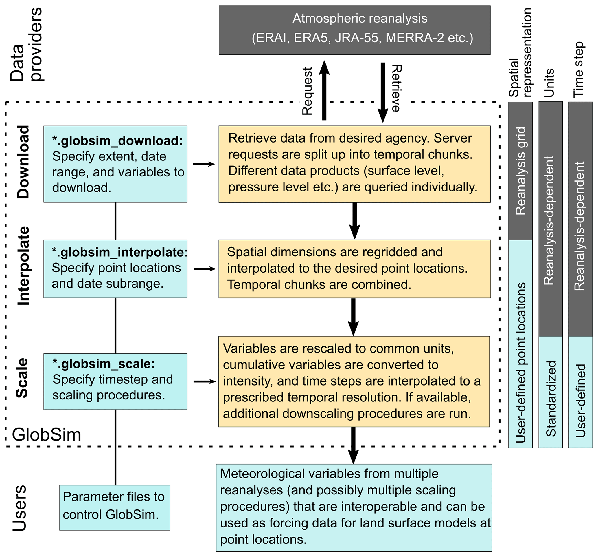
Figure 1GlobSim schematic: reanalysis data are processed in three main steps based on user-specified parameter files. The color of each box identifies user input and output (light blue), GlobSim processing (orange) and raw reanalysis data (grey).
Table 1Characteristics of the four reanalyses currently supported by GlobSim.

Complete ERA5 data from 1950 to the present are expected to be available in late 2019. ERAI is ERA-Interim, SA is surface analysis, SF is surface forecast, and PL is pressure level. ECMWF is the European Centre for Medium-Range Weather Forecasts, JMA is the Japan Meteorological Agency, and NASA is the National Aeronautics and Space Administration. In ERAI, the temporal resolution of surface forecasts is 6-hourly for instantaneous variables (e.g., temperature and air pressure) and 3-hourly for the accumulated variables (e.g., precipitation, short- and longwave radiation.)
3.2 Reanalyses
The four reanalyses currently implemented in GlobSim (Table 1) are ERAI, ERA5, the Japanese 55-year Reanalysis (JRA-55) and the Modern-Era Retrospective analysis for Research and Applications, version 2 (MERRA-2). Earlier reanalyses, such as CFSR, ERA-40, JRA-25 and MERRA, were not implemented in GlobSim because they have either been superseded by newer products or have ended. During the writing of this contribution, the discontinuation of ERAI in 2019 has been announced.
ERAI has 60 levels in the vertical dimension, with the highest at 1 mb, and the data are interpolated to 37 pressure levels (Dee et al., 2011). A reduced Gaussian grid with approximately uniform 79 km (T255) spacing for surface and other grid-point fields is used. ERAI covers the period from 1 January 1979 to 2019. The data contain analyses (at 00:00, 06:00, 12:00 and 18:00 UTC) for surface and pressure levels, as well as forecasts of instantaneous (e.g., 2 m surface air temperature, air temperature and relative humidity) and accumulated (e.g., total precipitation and radiation components; from 00:00 and 12:00 UTC, in 3, 6, 9 and 12 h steps) variables.
ERA5 is the fifth-generation atmospheric reanalysis produced by ECMWF to replace ERAI. Data are currently available from 1979 onward and later in 2019 are expected to be available starting in 1950. ERA5 is produced with a horizontal resolution of 31 km, a temporal resolution of 1 h and 137 vertical model levels, although the output pressure levels are identical to ERAI (Hersbach and Dee, 2016). ERA5 assimilates improved input data that better reflect observed changes in climate forcing, as well as many new or reprocessed observations that were not available during the production of ERAI. It also provides an estimate of uncertainty based on a 10-member ensemble with a temporal resolution of 3 h and spatial resolution of 62 km (Albergel et al., 2018).
JRA-55 is produced using a four-dimensional data assimilation system that uses many types of satellite data (Kobayashi et al., 2015). It is the second Japanese atmospheric reanalysis and covers the period from 1958 to near-real time. JRA-55 has a spatial resolution of 1.25∘ for assimilation (TL319) and 37 vertical pressure levels (1000–1 mb) for most variables in upper air, except dew-point depression, specific humidity, relative humidity, cloud cover, cloud water, cloud liquid water and cloud ice, which are produced for 27 levels from 1000 to 100 mb, only. The temporal resolution is 6 h for all levels and data (Kobayashi et al., 2015).
MERRA-2 replaces the original MERRA reanalysis (Gelaro et al., 2017) and uses the Goddard Earth Observing System-5 (GEOS-5) general circulation model (GCM) (Molod et al., 2015). It uses the cubed-sphere grid of Putman and Lin (2007) and has a spatial resolution of 0.5∘ × 0.625∘ (latitude × longitude, ∼ 50 km). MERRA-2 has 42 consistent pressure levels from the surface up to 0.1 mb (Gelaro et al., 2017). It has a temporal resolution of 6 h for the pressure-level data and 1 h for surface and forecast analysis.
3.3 Operation
3.3.1 Download
GlobSim downloads reanalysis data from each sponsoring agency (Table 1). Downloads are mediated through application program interfaces (APIs) which allow scripting access to data servers through Python. Server requests are split into temporal chunks in order to efficiently download large datasets. Different types of data (surface analysis, surface forecasts and pressure-level analysis) are queried individually. The outputs are stored as NetCDF4 files for each temporal chunk and reanalysis field, retaining the structure and conventions used by the sponsoring agencies.
3.3.2 Interpolation
GlobSim spatially interpolates gridded variables to the latitude and longitude of point locations using bilinear interpolation through the Python interface (ESMPy) of the Earth System Modeling Framework (ESMF) toolkit (O'Kuinghttons et al., 2016). Pressure-level variables are also interpolated spatially on each pressure level and in a subsequent step, vertical interpolation is performed at that location. First, geopotential height is normalized to obtain pressure-level elevation (E) (m) for each time step:
where ϕ is the geopotential height (m2 s−2) and g0 is the acceleration due to gravity of 9.807 m s−2. Then, pressure-level variables are vertically interpolated to the desired elevation. Geopotential height and other pressure-level variables are linearly extrapolated to locations where the pressure is greater than that of the lowest level with reanalysis data based on the values of the two lowest available pressure levels (Yessad, 2018). Although the 3-D interpolation combining surface and pressure-level information is not demonstrated here due to the relatively flat study area, it will be useful for further development of GlobSim by integrating additional scaling methods.
3.3.3 Scaling
We use the term “scaling” to describe the conversion of variables and units from their reanalysis-specific origins to a common standard as well as the possible application of additional temporal interpolation and downscaling procedures to produce data at fine spatial and temporal scales. For example, 3-hourly shortwave radiation from reanalyses can be interpolated to hourly resolution and used at mountain locations. When, additionally, fine-scale terrain–Sun geometry and horizon shading are taken into account, the resulting data are likely to be more accurate (Fiddes and Gruber, 2014).
The output variables of GlobSim are named following CF conventions (v1.6) with standard_name attributes that are consistent with the units used in the UDUNITS packages. The units of meteorological variables are first converted to the standard ones and then interpolated to achieve the required temporal resolution. Some of the forecast variables are not directly obtained from the reanalyses but instead are derived based on calculations involving other available variables (e.g., wind speed may be calculated from its northward and eastward components).
All analyzed fields in ERAI (e.g., surface analysis and pressure levels) and many forecast fields (e.g., temperature) are instantaneous. Some forecast variables (e.g., precipitation amount, surface downwelling longwave flux in air), however, are provided as accumulations in the reanalyses (Fig. 2). This means that each value is described as a change relative to another time in the forecast cycle instead of as an instantaneous flux. In contrast to the other reanalyses, the forecasts in ERAI are accumulated from the beginning of the respective forecast cycle (i.e., from 00:00 or 12:00 UTC; the solid blue lines in Fig. 2) rather than from the last step of the previous forecast cycle.
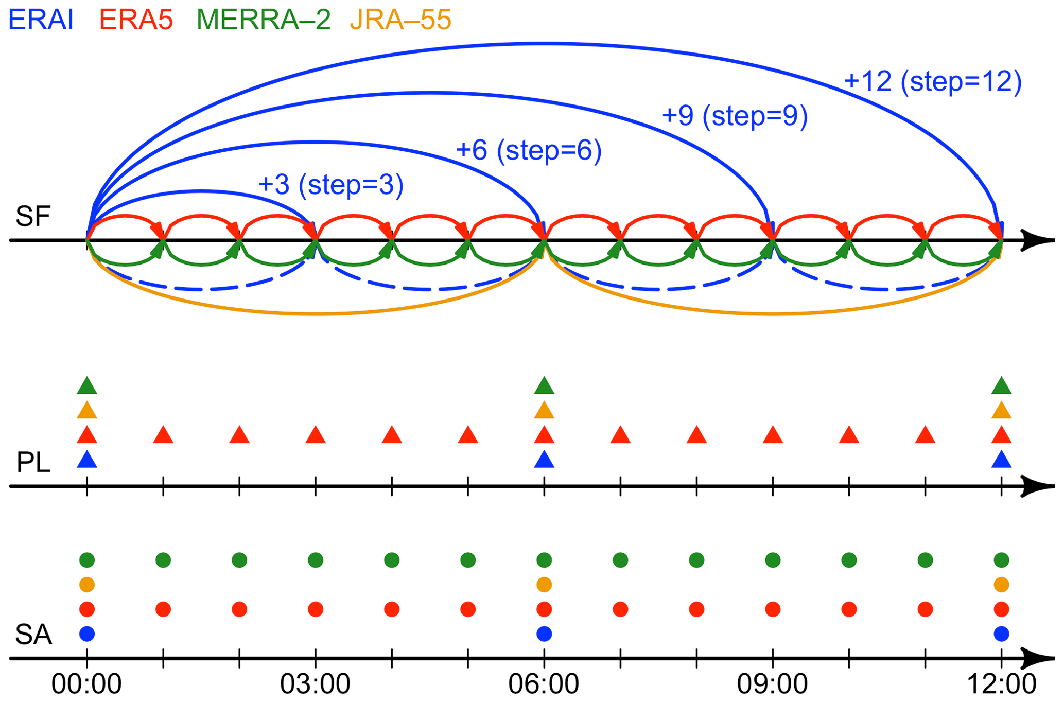
Figure 2The representation of surface analysis (SA), surface forecast (SF) and pressure-level (PL) data in the four reanalyses supported by GlobSim. The circles and triangles represent instantaneous variables which are reported at specific temporal resolutions. The lines represent accumulated variables in the forecasts which are reported as the integral of a flux over the time interval spanned by each arrow. Because the surface forecasts in ERAI are accumulated from the beginning of the respective forecast cycle (the solid blue lines) rather than from the end of the previous step, they must be disaggregated (the dashed blue lines) using Eq. (2) to prevent overlap in the integration periods.
In the scaling procedure, ERAI forecasts are first disaggregated to total amounts starting from the end of each previous step (the dashed blue lines in Fig. 2) for respective forecast cycle (00:00 and 12:00 UTC) and can be expressed as
where I denotes values spatially interpolated from the reanalysis grid (see Sect. 3.3.2), and S is the scaled results for that point location. The subscript s denotes the step and d the disaggregated value. The accumulated variables in forecasts are then converted to averages at the prescribed time resolution by dividing the length of the time step:
where the temporal scale factor (tn) could be given as
where tres and tout is the raw temporal resolution of reanalysis and required temporal resolution of outputs with the unit of hours (t). For ERAI, the disaggregated downwelling shortwave flux in air was found to be slightly negative ( W m−2) at some time steps. These values were interpreted to be artifacts and set to zero.
The surface downwelling longwave flux in air (LWd) is not directly available from MERRA-2 and is instead calculated as the sum of the longwave flux emitted from surface (LWe) and the surface net downward longwave flux (LWn):
In ERAI, relative humidity (RH) (%) is derived by following Lawrence (2005):
where Ta (K) is the near-surface air temperature and Td (K) is the dew-point temperature. Wind speed and direction are calculated from the eastward (U) and northward (V) components:
and
where Ws is the wind speed in m s−1, Wd is wind direction in degrees and atan 2 is the two-argument arctangent used to compute an unambiguous angle when converting from Cartesian to polar coordinates.
Reanalysis products are carefully designed and tested before release. In addition, many studies have evaluated their performance by intercomparison, by comparison with observations (e.g., Jiang et al., 2015) and by applying them to model simulations (e.g., Albergel et al., 2018; Beck et al., 2019). For this reason, we focus on the application of GlobSim for demonstration rather than the direct testing of reanalysis variables or their interpolated products. An intercomparison of GlobSim-derived meteorological variables for the test area (Fig. 3) helps to appreciate differences or detect blunders in conversion. Below, we use GlobSim to drive ground-surface temperature (GST) simulation using a permafrost/land-surface model for a remote location in northern Canada underlain by permafrost. We then analyze ensemble results and their deviance from observations.
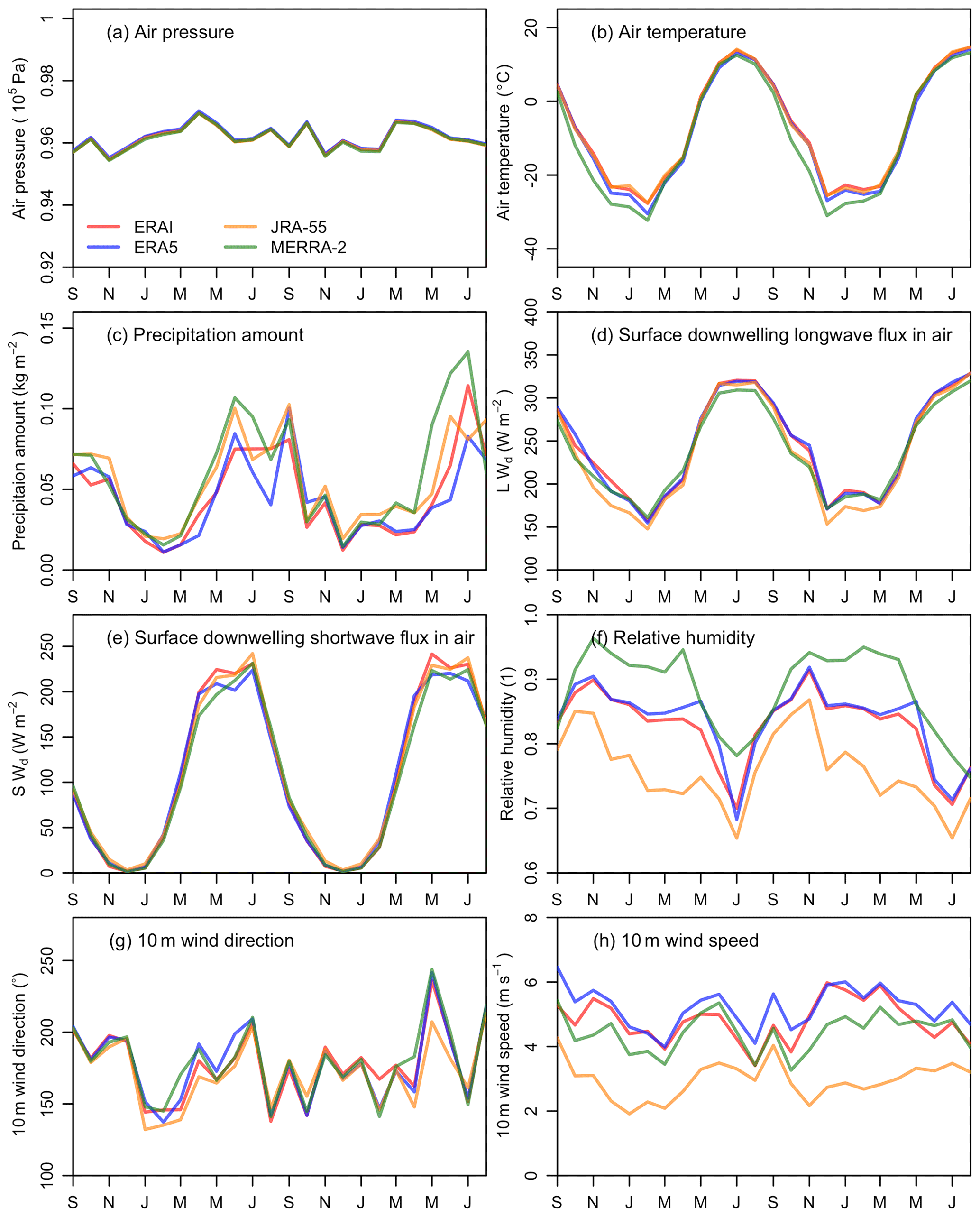
Figure 3Intercomparisons of monthly variables derived from GlobSim which are used in GEOtop during the period September 2015–August 2017. SWd and LWd is the surface downwelling shortwave flux in air and downwelling longwave flux in air, respectively.
4.1 Study area
The research area is centered at 64∘42′ N, 110∘36′ W, near the north shore of Lac de Gras in the Northwest Territories, Canada (Fig. 4). The area is located within the zone of continuous permafrost, the mean annual air temperature (MAAT) is −9.0 ∘C and the total annual precipitation is 284 mm during September 1998–August 2007 (Ekati A; Environment Canada, 2019), with about 50 % occurring as snow (Jones et al., 2003). Typically, snow cover lasts for about 7 months and because of strong winds (Hu et al., 2003), snow depth shows strong spatial variability; it is shallowest in much of the higher-elevation, convex terrain (e.g., tops of eskers) and deepest in low-lying areas with taller shrub vegetation or in the lee of larger terrain features (Holubec et al., 2003).
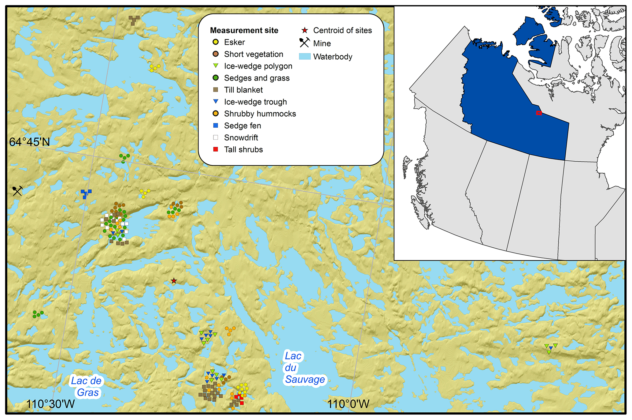
Figure 4Study area and approximate location of measurement sites. Many point locations overlap at the scale of the map, so the positions of their markers have been dispersed to better illustrate the number and type of sites. The centroid of all measurement sites (red star) was used as the location for which GlobSim reanalysis data were derived. The top right inset map shows the location of the study area (red square) within the Northwest Territories (blue region) of Canada. The elevation tinted hillshade basemap is provided by the Natural Resources Canada Federal Geospatial Platform Elevation Data Web Mapping Service and is derived from the Canadian Digital Elevation Model (CDEM). Water-body outlines were obtained from the ArcGIS online data library.
The area has undulating to moderately rugged topography dominated by glacial features (Kerr et al., 1997; Dredge et al., 1999), mostly on the order of 10–20 m in relief (Dredge et al., 1999) and composed of glacial till (Haiblen et al., 2018). Till deposits are described according to their thicknesses, as veneers (< 2 m), blankets (2–10 m) or hummocky (5–30 m). Eskers are the prevalent glaciofluvial deposits, reaching heights of 35 m and occasionally containing massive ice on the order of 2–5 m thick (Haiblen et al., 2018; Wolfe et al., 1997). The poorly drained low-lying areas have peat deposits and are generally associated with ice-wedge polygons. The region is within the southern Arctic ecozone described by continuous shrub tundra (Wiken et al., 1996). The most common shrubs are dwarf birch (Betula pumila) and Labrador tea (Ledum decumbens). Uplands are well drained with lichen and mosses, whereas wetlands are typically colonized with sedges and mosses.
4.2 Observations and quality control
GST was measured at 156 locations in order to capture the fine-scale spatial variability and to test the performance of GlobSim in supporting GST simulation beneath different terrain classes. Study plots measuring 15 m × 15 m were established that reflect the different terrain types in the area (Gruber et al., 2018). Each plot was instrumented with three to four temperature loggers approximately 0.1 m below the ground surface. Site characteristics including surficial geology, topography and snow deposition tendency were recorded for each study plot, and subplot characteristics were collected for each logger at the 1 m × 1 m scale including drainage tendency, vegetation height and leaf area index (LAI). Surface air temperature is measured at six locations, equally distributed between topographic high and low points. Sensors are mounted in passively ventilated radiation shields (Young, model 41003) 2–3 m above the ground surface.
This study uses temperature measurements over 2 years (September 2015–August 2017) and annual mean values described here refer to measurements beginning in September and ending in August of the following year. GST data loggers (GeoPrecision, model M-Log5W-SIMPLE) and surface air temperature loggers (GeoPrecision, model M-Log5W with a Rotronic Hygroclip sensor) have a resolution of 0.01 ∘C and an accuracy of ±0.1 ∘C. All measurements have intervals of 20 min.
4.3 Distinguishing terrain types
The variability of GST regimes near Lac de Gras is controlled by many factors, the most significant of which are surficial geology, vegetation type and height and topography (cf. Hu et al., 2003). The 156 sites are hence grouped into 10 classes based on surface and subsurface characteristics as described at a scale of 15 m × 15 m (Fig. 5). This classification is subjective and was developed to identify common terrain types that could be easily recognized in the field and that explain a significant part of the observed spatial variation of GST. Surface offset is used here to quantify local ground temperature variations (Smith and Riseborough, 2002). It is defined as , where MAGST is the mean annual ground-surface temperature and MAAT is the mean annual air temperature.

4.4 Process-based numerical model
GEOtop (version 2.0), a physically based numerical model, is used for this demonstrator application because it describes the complex abiotic processes in permafrost environments well (e.g., Endrizzi and Marsh, 2010; Gubler et al., 2013; Endrizzi et al., 2014; Pan et al., 2016). It represents the heat and water transfer in soil as well as the energy transfer between the soil and the atmosphere. Additionally, it solves equations describing the interactions of water and energy during soil freezing and thawing (Dall'Amico et al., 2011; Endrizzi and Gruber, 2012) and simulates the water and energy transfer in the snow cover. GEOtop, driven by ERA-Interim forcing data, was found to be suitable for reproducing ground temperature observations (Mugford et al., 2012; Fiddes et al., 2015).
4.5 Model settings and parameters
GEOtop was forced by the four reanalyses obtained via GlobSim, providing hourly data for precipitation, wind velocity, wind direction, short- and longwave radiation, relative humidity and near-surface air temperature. Given the gentle topography and small test area, the time series were derived for the geographic center of measurement sites, only (Fig. 4). Model parameters and initial conditions were specified for each terrain type based on field observations. For example, the uppermost soil type was derived from drill logs and soil pit measurements (Table 2). Vegetation height was measured within each 1 m × 1 m subplot around the data logger (Table 3). Some parameters, which are challenging to measure directly, were then subsequently refined, within the range of plausible values (cf. Gubler et al., 2013), through experimentation with the model. The snow correction factor, which scales the simulated amount of snow via precipitation amount, is used to capture the differences among the 10 terrain classes. It was determined by fitting the simulated melt-out date of the snow (Schmid et al., 2012) to observations (Fig. 6). Snow blowing is parameterized as wind compaction in 1-D (Pomeroy et al., 1993) for all the terrain types except the tall shrub site.
Table 2GEOtop soil parameters used to simulate different stratigraphic units.
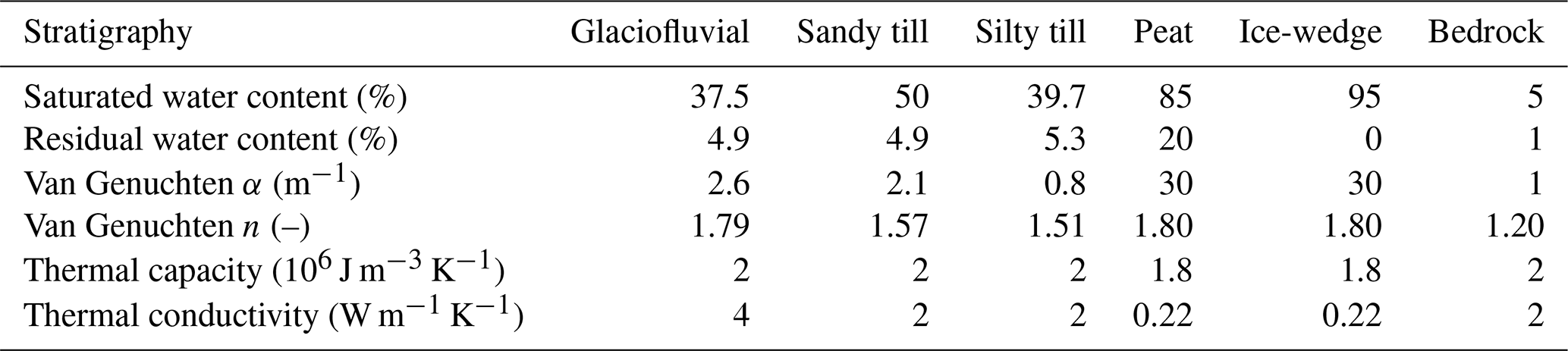
Table 3GEOtop parameters for different terrain types.
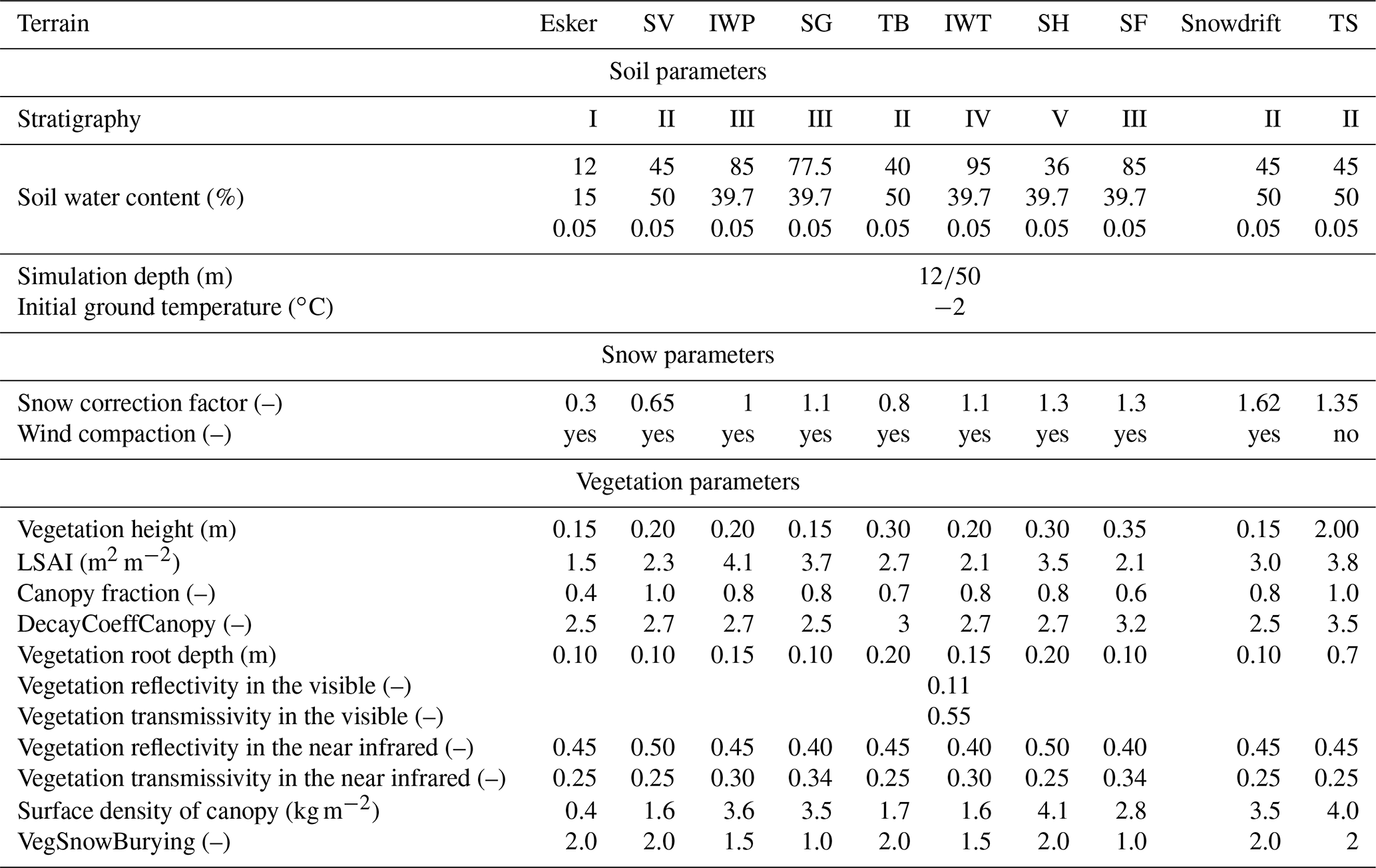
SV is short vegetation, IWP is ice-wedge polygon, SG is sedges and grass, TB is till blanket, IWT is ice-wedge trough, SH is shrubby hummock, SF is sedge fen, and TS is tall shrub. The soil water content is specified for each soil layers present in Fig. 7. DecayCoeffCanopy is the decay coefficient of the eddy diffusivity profile in the canopy, and VegSnowBurying is the coefficient of the exponential snow burying of vegetation. The different stratigraphic profiles are listed in Fig. 7. The simulation depths of 12 and 50 m were used for GST and long-term simulations, respectively.
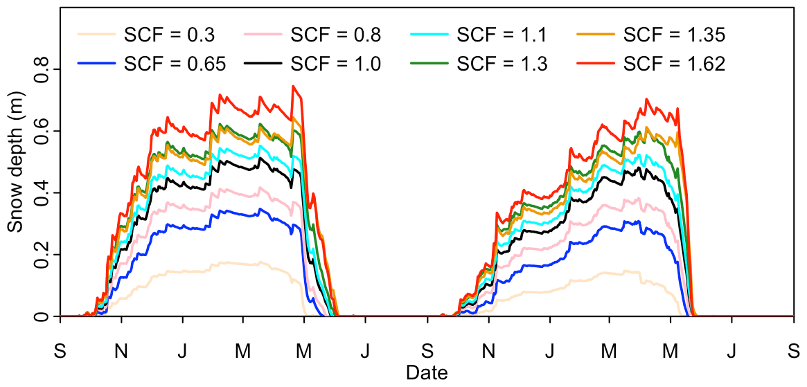
Figure 6Simulated ensemble mean daily snow depth using different snow correction factors (SCFs) to reproduce the snow melt-out date for terrain types during the period September 2015–August 2017. Max is the maximum snow depth during the measured period in meters.
Soil parameters were estimated based on soil textural data collected at each plot (Subedi, 2016). More specifically, the soil particle thermophysical properties (e.g., thermal conductivity and heat capacity) were estimated based on typical values for common material types in each unit. The soil freezing characteristic curve parameters (van Genuchten α, van Genuchten n, saturated and residual water content) for rock and organic material were taken from Gubler (2013). For mineral soil, values were obtained by averaging the soil textural data within each class and applying the ROSETTA model v3.0 (Zhang and Schaap, 2017). For the ice-wedge trough, the uppermost layer was assigned a the water/ice content of 95 % to simulate the ice-wedge itself. Leaf and stem area index (LSAI) and surface density of canopy were estimated based on measured LAI and moss thickness. Canopy fraction was determined based on plot photos (Gruber et al., 2018). Although the same vegetation reflectivity (0.11) and transmissivity (0.15) was used for each terrain type, overall reflectivity and transmissivity are in fact dependent on vegetation and subsurface conditions.
A lower boundary condition of zero heat flux was used for these shallow simulation. Although borehole analysis revealed a heat flow of 0.046 W m−2 based on temperature measurements in two deep boreholes near Lac de Gras (Mareschal and Jaupart, 2004), it is not appropriate to apply these measurements to the shallow profile simulations because of the transient changes in the temperature profile near the surface during recent decades. We use 30 soil layers with a total depth of 12 m (Fig. 7) and an initial soil temperature of −2 ∘C. Reanalyses data for July 2000–June 2010 were used to spin up the model by running it 10 times (100 years) before simulations were conducted from July 2010 onward.
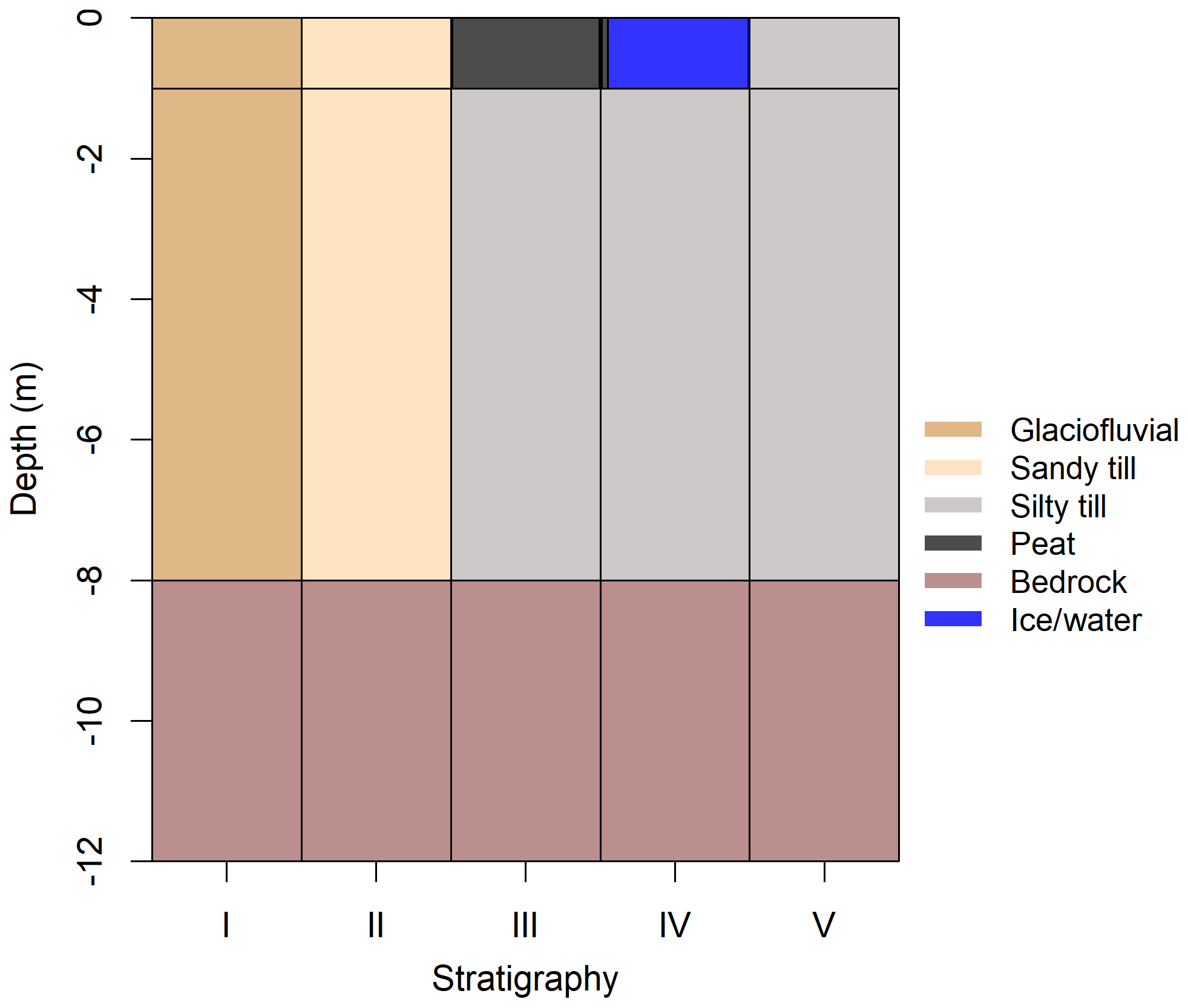
Figure 7Soil profiles for the different terrain types used to partition surface temperature observations. Parameters for each of the subsurface materials are provided in Table 2. The stratigraphic unit (I–V) associated with each of the terrain types is listed in Table 3. In the long-term simulation, the layer of bedrock is extended to 50 m.
Reanalysis produces multi-decadal meteorological variables (Table 1), and this makes simulating long-term changes of land-surface processes possible. To demonstrate the utility of GlobSim for supporting long-term simulation, we conducted an additional deep ground temperature simulation from 1980 to 2017 for a single terrain type. The soil profile increased to 60 layers with a total depth of 50 m via expending the bedrock layer. The model was spun up by repeating the reanalysis of January 1980–December 1984 100 times (500 years). To improve simulation efficiency, we simplified GEOtop simulation by assuming the vegetation and soil moisture were constant over time. This is warranted, as we aim to simply demonstrate the potential for long-term application.
4.6 Comparison of observation and simulation
To compare simulations with observations, the mean bias (BIAS) and root mean squared error (RMSE) were computed for each time series as
and
where Tmod is the modeled temperature, Tobs is the observed temperature, and N is the total number of measurements.
5.1 Observed temperature
During the 2 years measured, the MAGST (SO) at individual sites span a large range of 11.43 ∘C, from −8.03 (0.46) ∘C on an esker with low vegetation, soil moisture and snow cover (Fig. 6), to 3.40 (11.89) ∘C in the tall shrubs, which retain snow (Fig. 5, Table 4). Daily GST shows seasonal patterns that are similar for each terrain type, MAGST ranges within terrain types are reduced to 1.19–6.50 ∘C, and mean surface offsets differ clearly.
Table 4Summary of temperatures in the 10 terrain types.
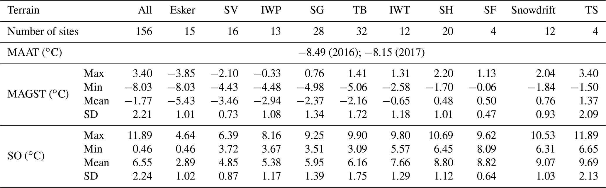
MAAT is mean annual air temperature, MAGST is mean annual ground-surface temperature, and SO is surface offset.
The surface air temperature is best approximated by ERA5, which has the lowest daily RMSE of 1.94 ∘C and bias of 0.15 ∘C, while MERRA-2 was the worst with an RMSE of 3.65 ∘C and a bias of −1.62 ∘C (Table 5). During 2015–2017, the mean MAAT derived from the four reanalyses was ∘C, which is in good agreement with the observed MAAT of −8.32 ∘C. The ensemble mean, which had a daily RMSE of 1.87 ∘C, outperformed all individual reanalyses during the measured period and reduced RMSE by 0.07–1.78 ∘C (Fig. 8).
Figure 8c–l compare the daily ensemble means of simulated GST to observation means for the 10 terrain types. The performance varies significantly among terrain types and reanalyses, with the RMSE ranging from 1.09 to 3.00 ∘C (Table 5). Even within the same terrain class, the mean RMSE difference for the four reanalyses was 0.60±0.22 ∘C and was up to 0.89 ∘C for the sedge fen terrain type. The overall RMSE for the four reanalyses was 1.96 ∘C for daily means and 0.92 ∘C for annual means.
Most (81 %) of the simulated daily GST is within the observation range, although the spread in simulated values is generally smaller than in observations (Fig. 8). The spread of model results is generally greatest sometime between January and May of each year, with the exact timing depending on the terrain type. The variability of observations also depends on the terrain type, with the lowest variability at sedge fen sites and the greatest at till blanket sites. The ensemble mean shows good agreement with the observation mean, with RMSE ranging from 1.02 to 2.45 ∘C depending on the terrain type.
The GST ensemble mean usually performed better compared to the individual ensemble members based on single reanalyses, as was the case with surface air temperature. For 6 of 10 terrain types, the simulated GST ensemble mean achieved better results based on the RMSE. Moreover, the ensemble mean had the smallest RMSE for the daily GST when averaged over all sites. Consequently, the RMSE was reduced by 0.01–0.31 ∘C for daily GST and by 0.00–1.01 ∘C for SO as a whole (Fig. 9). Overall, simulations forced by MERRA-2 achieved the best performance for MAGST with the BIAS and RMSE of −0.03 and 0.75 ∘C, respectively. Compared to other individual reanalyses, the simulations forced by ERA5 often yield the second best RMSE (8∕14) if not the best (2∕14) (Table 5).
Table 5Deviance of simulations from the mean of observations within each terrain type. The smallest BIAS and RMSE values for each row are indicated in bold font.
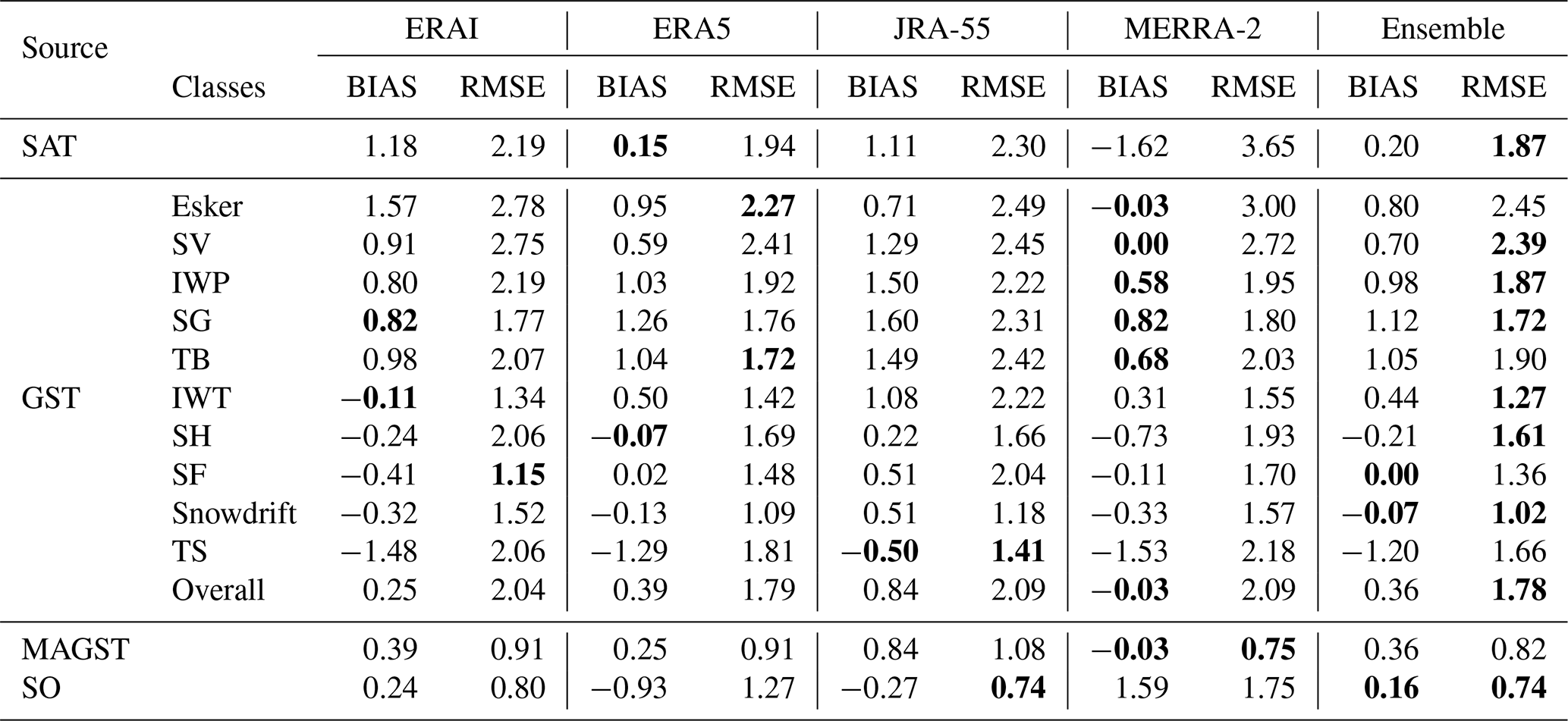

Figure 8Comparison of ensemble (ENS) simulation results with observations (OBS) for (a) daily near-surface air temperature (SAT); (b) daily ground-surface temperature (GST) for all the sites and; (c–l) daily GST for individual terrain classes. The date range for all figures is September 2015 to September 2017.
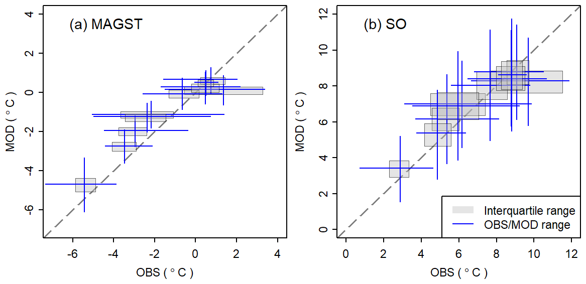
Figure 9Comparison of ensemble results and observations for (a) mean annual ground-surface temperature (MAGST) and (b) surface offset (SO) for the 10 terrain types.
The long-term simulation shows warming trends for MAAT and for modeled annual mean ground temperature (MGT) at all depths. The modeled warming rate of the ensemble mean was 0.42 ∘C per decade for MAAT and 0.42, 0.21 and 0.13 ∘C per decade for the annual mean ground temperature at depths of 0.1, 10 and 20 m, respectively (Fig. 10).
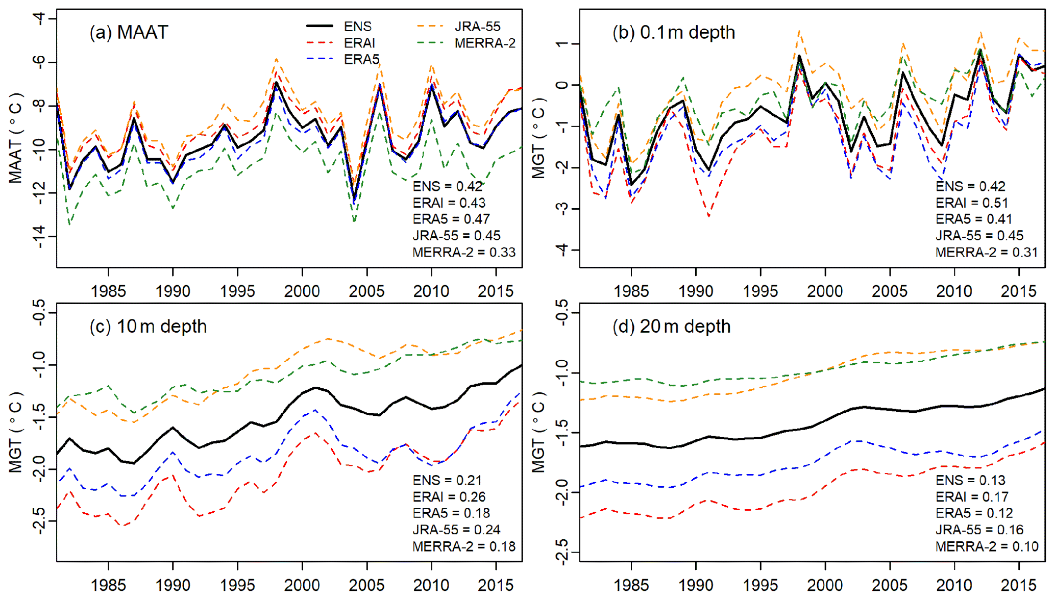
Figure 10Changes of (a) mean annual air temperature (MAAT) derived from reanalyses, modeled annual mean ground temperature (MGT) at the depth of (b) 0.1 m, (c) 10 m and (d) 20 m for shrubby hummocks (SH) terrain type of between 1980 and 2017. The numbers in the lower right of each figure correspond to the magnitude of the warming trend for each reanalysis and their ensemble mean with the unit of ∘C per decade. ENS corresponds to ensemble mean. The trend lines were calculated using a linear regression model, and all the slopes were statistically significant with p<0.05.
The observed spatial variability of GST, with MAGST difference up to 11.5 ∘C over 30 km, highlights the need for spatially differentiated simulation in order to represent the different thermal regimes among locations or terrain types as well as their different transient responses to climate forcing. The reduced standard deviation and range of observed MAGST within terrain types indicates that the classification method for terrain type used here is reasonable. Furthermore, it shows that conceptualizing and simulating GST via terrain types can be expected to explain a significant part of the variation observed.
The variables in GlobSim output are similar between reanalyses at one co-located point, indicating that major blunders are unlikely to exist in the GlobSim code. The data approximate surface air temperature near Lac de Gras well and GST simulation results from GEOtop agree well with observations both in terms of summary statistics (Table 5) and the reproduction of the underlying seasonal ground thermal regime (Fig. 8). While quality requirements and simulation quality will differ with application and geographic area, our demonstrator shows the suitability of reanalyses and GlobSim for driving process-based numerical simulation at a site scale. It shows that the combination of driving meteorological data, site conditions and a suitable model is able to reproduce spatial differences as well as the temporal evolution of ground temperature. The availability of multi-decadal reanalysis time series opens the door for better investigating transient processes and phenomena at and below the land surface. Ground temperature is one of many possible variables to investigate and in this study was chosen as an exemplar because it reflects the motivation and expertise of the authors.
The greatest model spread occurs between January and May when the thickness of the insulating snowpack accumulates differences in meteorological variables over the winter period and plays an important role in controlling ground temperature. This increase in model spread is also conspicuously absent in the esker terrain type, for which the effect of snow is minimal. The low variability of observed GST for the sedge fen terrain type may be due in part to the small number of measurement sites in this terrain type (n=4). However, the tall shrubs class has the same number of measurements and exhibits variability similar to other terrain types with a higher number of measurements (e.g., shrubby hummocks, n=20). This suggests that the observed spatial variation of GST in each terrain type is a good first-order indicator of its full range of variability.
The relatively small range of GST in the model ensemble when compared to the observations is likely due to the small number of simulations, in which only differing reanalyses are used but not perturbed physics or differing land-surface models. The large difference of RMSE for simulated ground-surface temperature based on the four forcing reanalyses indicates the potential uncertainty caused by forcing datasets. Ensemble means often achieve better performance compared to the individual ensemble members, indicating the potential of this approach to improve simulation results. Both findings underscore the value of using more than one reanalysis for driving simulation studies.
MERRA-2 underestimated surface air temperature near Lac de Gras, while the simulation overestimated the ground temperature. As a result, the BIAS of MAGST forced by MERRA-2 is very close to 0 and the RMSE is smallest due to opposing biases canceling out. This is also demonstrated by the highest RMSE of surface offset for MERRA-2.
7.1 Observed and simulated temperature
Our results highlighted the magnitude of spatial heterogeneity in ground temperature (see also Smith, 1975; Gubler et al., 2011; Schmid et al., 2012; Morse et al., 2012; Gisnås et al., 2014) over distances that usually are within single grid cells (30–100 km) of a reanalysis or climate model. When comparing grid-scale simulation results with point observations, this heterogeneity and scale mismatch usually confound model validation.
The ensemble ranges of modeled and observed GST (Fig. 8) reflect two distinct sources of variability. The former stems from differences in the forcing data, and the latter is due to terrain characteristics. However, both ranges inform how well a simulation would represent a particular type of location within the study area and while a direct comparison of the two ranges may not be valid, the observed variability helps contextualize the uncertainty introduced by the forcing data relative to changes in GST over as little as a few meters. From this study, we see that the relative importance of reanalysis uncertainty varies seasonally and spatially.
While we do not aim to evaluate the quality of reanalyses themselves, the calculated air temperature bias indicates how accurate reanalyses and GlobSim are for our study area. It is therefore worthwhile to contextualize these results with those of studies dedicated to a formal evaluation of the reanalyses. For example, in Greenland, Reeves Eyre and Zeng (2017) found average monthly SAT biases averaged over all stations of 0.81 ∘C (MERRA-2), 1.76 ∘C (ERAI) and 1.95 ∘C (JRA-55). Wang and Zeng (2012) found a daily average bias for ERAI over 63 stations on the Tibetan Plateau of 3.21 ∘C, while an analysis of individual stations within North America found 6-hourly ERAI bias values to mostly fall between −1.5 and 4.5 ∘C but were as large as 7.5 ∘C (Decker et al., 2012). The SAT bias calculated at our sites ranges from −1.62 ∘C (MERRA-2) to 1.18 ∘C (ERAI) (Table 5). The numbers of this and previous studies remind us that the application of reanalyses for simulating surface phenomena is bound to be imperfect and that the success of application in one area cannot be transferred to other areas uncritically.
7.2 Advantages and limitations of GlobSim
Previous work has investigated parameter uncertainty with ensemble simulation (Harp et al., 2016; Gubler et al., 2013) but not investigated the effect of uncertainty in the forcing data. Other studies have used multiple forcing datasets to drive ensembles at the grid scale. Jafarov et al. (2012) used a five-member GCM composite product for driving a permafrost model on a 2 km × 2 km grid using mean monthly air temperature and precipitation. Here, the coarse temporal resolution and the GCM-specific realization of weather events preclude some types of detailed investigation with observations. Guo et al. (2017) used three different reanalyses to evaluate the effect of forcing data on permafrost model uncertainty on a 0.5∘ × 0.5∘ grid, excluding fine-scale variation. For simulation at finer scales, dynamic and/or statistical downscaling of GCM and regional climate model (RCM) outputs has been used (Salzmann et al., 2007; Marmy et al., 2016). The downscaling and debiasing, however, are often limited to areas with detailed observations.
Although the demonstrator presented here is relatively simple, it addresses a critical gap in permafrost research and likely for other modeling communities as well. It provides a basis upon which to implement improved downscaling methods and to work towards debiasing GCM results with reanalyses (Cannon, 2016) at the point scale. Specifically, GlobSim helps to (1) fill gaps in meteorological observations caused by instrument failure, (2) evaluate models at locations where observations to compare with model results (ground temperature in this demonstrator) are available, but meteorological observations to drive models are lacking and (3) predict environmental phenomena that are driven by atmospheric conditions (permafrost in this demonstrator) at locations for which no observational data exist. Such predictions could also support the analysis and interpretation of field manipulation experiments or long-term monitoring data. In keeping with the permafrost example, these experiments could investigate the effects of vegetation change or different snow management practices (O'Neill and Burn, 2017). In remote locations, long-term meteorological observations are sparse, which limits the application of models that require detailed inputs. The recent publication of two such datasets illustrates the importance – and the general lack – of complete records which can be used to both force and evaluate models (Boike et al., 2019, 2018). While the methods contained in GlobSim are simple, it nevertheless provides an important simplification of the application of reanalysis data toward simulation studies outside atmospheric science. As GlobSim outputs use the CF conventions (Hassell et al., 2017), it contributes to the ease of using multiple data sources.
Our results have demonstrated the performance of GlobSim for site-level simulation in one particular field area with gentle topography. Simulation accuracy for other areas and application will differ, especially in mountains and near coasts where topography and other heterogeneity presents additional challenges for downscaling. Additional scaling rules such as TopoScale (Fiddes and Gruber, 2014), REDCAPP (Cao et al., 2017) or those implemented in MSDH (Sen Gupta and Tarboton, 2016) may be added in the future, making GlobSim more suitable in mountains.
7.3 ERA5 ensemble
ERA5 provides uncertainty estimates for all parameters at 3 h intervals and at a horizontal resolution of 62 km. This is achieved using an ensemble of 10 members that differ in their assimilated observations, initial conditions and model structure. In other words, ERA5 itself is an ensemble simulation. In GlobSim, only the ensemble mean of ERA5 is currently used. In a next step, efforts will be devoted to compare ensembles of ERA5 and fully incorporate them into GlobSim.
We describe and test the software GlobSim, which has been designed to support ensemble simulations at a the site level. Specially, GlobSim is designed to easily retrieve, interpolate and scale reanalyses in order to produce time series of meteorological variables with common structure, temporal resolution and units. It currently supports four reanalyses: ERAI, ERA5, JRA-55 and MERRA-2. We demonstrate the utility of GlobSim by driving a model of ground-surface temperature in a tundra environment with permafrost and comparing its output to observations. Our results support three conclusions:
- 1.
GlobSim improves the usability of reanalyses for land-surface simulations by deriving time series of climate variables in uniform format from multiple reanalyses for point locations.
- 2.
GlobSim enables efficient ensemble simulations at single or multiple points.
- 3.
Compared to simulations forced by individual reanalyses, ensemble means often yielded better performance with reduced RMSE in addition to providing information about predictive uncertainty.
GlobSim is developed as a Python package available at Zenodo (https://doi.org/10.5281/zenodo.3237258, last access: 30 October 2019) as a GPL-3.0 project in the version published here and with documentation at GitHub (http://github.com/geocryology/globsim, last access: 30 October 2019). A docker container containing the required libraries is also available at GitHub (https://hub.docker.com/r/geocryology/globsim, last access: 30 October 2019). The ESMF library was downloaded from http://earthsystemcog.org/projects/esmf/ (last access: 30 October 2019).
Observations are available from the Nordicana-D data repository (Gruber et al., 2018, https://doi.org/10.5885/45561XX-2C7AB3DCF3D24AD8,).
BC carried out this study by analyzing data, developing part of the GlobSim code and performing the simulations. XQ contributed to the development and design of GlobSim. NB contributed to the development and testing of GlobSim, supported the operation of GEOtop on the virtual machines, tested the initial GlobSim parameters and conducted the field measurements. ESJ contributed to the collection of field measurements, developed the terrain-type classifications and assisted with the selection of model parameters. SG conceived and guided the project, and designed the initial code of GlobSim. All authors contributed to the writing and editing of the manuscript.
The authors declare that they have no conflict of interest.
The authors thank Carleton Research Computer Services for their support of this project and acknowledge the support of Ryan O'Kuinghttons and Robert Oehmke in finding a good way to use it for efficient interpolation in GlobSim. Luis Padilla-Ramirez provided valuable testing, feedback and bug fixing.
This research has been supported by the Southern Ontario Smart Computing Innovation Platform (SOSCIP)/Ontario Centres of Excellence (OCE)/IBM (grant no. 806522) and the Natural Sciences and Engineering Research Council of Canada (grant no. RGPIN-2015-06456).
This paper was edited by David Lawrence and reviewed by two anonymous referees.
Albergel, C., Dutra, E., Munier, S., Calvet, J.-C., Munoz-Sabater, J., de Rosnay, P., and Balsamo, G.: ERA-5 and ERA-Interim driven ISBA land surface model simulations: which one performs better?, Hydrol. Earth Syst. Sci., 22, 3515–3532, https://doi.org/10.5194/hess-22-3515-2018, 2018. a, b, c
Arsenault, K. R., Kumar, S. V., Geiger, J. V., Wang, S., Kemp, E., Mocko, D. M., Beaudoing, H. K., Getirana, A., Navari, M., Li, B., Jacob, J., Wegiel, J., and Peters-Lidard, C. D.: The Land surface Data Toolkit (LDT v7.2) – a data fusion environment for land data assimilation systems, Geosci. Model Dev., 11, 3605–3621, https://doi.org/10.5194/gmd-11-3605-2018, 2018. a
Beck, H. E., Pan, M., Roy, T., Weedon, G. P., Pappenberger, F., van Dijk, A. I. J. M., Huffman, G. J., Adler, R. F., and Wood, E. F.: Daily evaluation of 26 precipitation datasets using Stage-IV gauge-radar data for the CONUS, Hydrol. Earth Syst. Sci., 23, 207–224, https://doi.org/10.5194/hess-23-207-2019, 2019. a
Benestad, R. E., Hanssen-Bauer, I., and Chen, D.: Empirical-Statistical Downscaling, World Scientific, https://doi.org/10.1142/6908, 2008. a
Bieniek, P. A., Bhatt, U. S., Walsh, J. E., Rupp, T. S., Zhang, J., Krieger, J. R., and Lader, R.: Dynamical downscaling of ERA-Interim temperature and precipitation for Alaska, J. Appl. Meteorol. Climatol., 55, 635–654, https://doi.org/10.1175/JAMC-D-15-0153.1, 2016. a
Boike, J., Juszak, I., Lange, S., Chadburn, S., Burke, E., Overduin, P. P., Roth, K., Ippisch, O., Bornemann, N., Stern, L., Gouttevin, I., Hauber, E., and Westermann, S.: A 20-year record (1998–2017) of permafrost, active layer and meteorological conditions at a high Arctic permafrost research site (Bayelva, Spitsbergen), Earth Syst. Sci. Data, 10, 355–390, https://doi.org/10.5194/essd-10-355-2018, 2018. a
Boike, J., Nitzbon, J., Anders, K., Grigoriev, M., Bolshiyanov, D., Langer, M., Lange, S., Bornemann, N., Morgenstern, A., Schreiber, P., Wille, C., Chadburn, S., Gouttevin, I., Burke, E., and Kutzbach, L.: A 16-year record (2002–2017) of permafrost, active-layer, and meteorological conditions at the Samoylov Island Arctic permafrost research site, Lena River delta, northern Siberia: an opportunity to validate remote-sensing data and land surface, snow, and permafrost models, Earth Syst. Sci. Data, 11, 261–299, https://doi.org/10.5194/essd-11-261-2019, 2019. a
Cannon, A. J.: Multivariate bias correction of climate model output: Matching marginal distributions and intervariable dependence structure, J. Climate, 29, 7045–7064, https://doi.org/10.1175/JCLI-D-15-0679.1, 2016. a
Cao, B., Gruber, S., and Zhang, T.: REDCAPP (v1.0): parameterizing valley inversions in air temperature data downscaled from reanalyses, Geosci. Model Dev., 10, 2905–2923, https://doi.org/10.5194/gmd-10-2905-2017, 2017. a, b, c, d
Dall'Amico, M., Endrizzi, S., Gruber, S., and Rigon, R.: A robust and energy-conserving model of freezing variably-saturated soil, The Cryosphere, 5, 469–484, https://doi.org/10.5194/tc-5-469-2011, 2011. a
Daly, C., Halbleib, M., Smith, J. I., Gibson, W. P., Doggett, M. K., Taylor, G. H., Curtis, J., and Pasteris, P. P.: Physiographically sensitive mapping of climatological temperature and precipitation across the conterminous United States, Int. J. Climatol., 28, 2031–2064, https://doi.org/10.1002/joc.1688, 2008. a, b
Decker, M., Brunke, M. A., Wang, Z., Sakaguchi, K., Zeng, X., and Bosilovich, M. G.: Evaluation of the Reanalysis Products from GSFC, NCEP, and ECMWF Using Flux Tower Observations, J. Climate, 25, 1916–1944, https://doi.org/10.1175/JCLI-D-11-00004.1, 2012. a, b, c
Dee, D. P., Uppala, S. M., Simmons, A. J., Berrisford, P., Poli, P., Kobayashi, S., Andrae, U., Balmaseda, M. A., Balsamo, G., Bauer, P., Bechtold, P., Beljaars, A. C. M., van de Berg, L., Bidlot, J., Bormann, N., Delsol, C., Dragani, R., Fuentes, M., Geer, A. J., Haimberger, L., Healy, S. B., Hersbach, H., Hólm, E. V., Isaksen, L., Kållberg, P., Köhler, M., Matricardi, M., McNally, A. P., Monge-Sanz, B. M., Morcrette, J.-J., Park, B.-K., Peubey, C., de Rosnay, P., Tavolato, C., Thépaut, J.-N., and Vitart, F.: The ERA-Interim reanalysis: configuration and performance of the data assimilation system, Q. J. Roy. Meteor. Soc., 137, 553–597, https://doi.org/10.1002/qj.828, 2011. a, b
Dredge, L. A., Kerr, D. E., and Wolfe, S. A.: Surficial materials and related ground ice conditions, Slave Province, N. W.T., Canada, Can. J. Earth Sci., 36, 1227–1238, 1999. a, b
Ekici, A., Chadburn, S., Chaudhary, N., Hajdu, L. H., Marmy, A., Peng, S., Boike, J., Burke, E., Friend, A. D., Hauck, C., Krinner, G., Langer, M., Miller, P. A., and Beer, C.: Site-level model intercomparison of high latitude and high altitude soil thermal dynamics in tundra and barren landscapes, The Cryosphere, 9, 1343–1361, https://doi.org/10.5194/tc-9-1343-2015, 2015. a
Endrizzi, S. and Gruber, S.: Investigating the effects of lateral water flow on the spatial patterns of thaw depth, in: Proceedings of the 10th International Conference on Permafrost, 25–29 June 2012, 91–96, Salekhard, Russia, 2012. a
Endrizzi, S. and Marsh, P.: Observations and modeling of turbulent fluxes during melt at the shrub-tundra transition zone 1: point scale variations, Hydrol. Res., 41, 471–491, https://doi.org/10.2166/nh.2010.149, 2010. a
Endrizzi, S., Gruber, S., Dall'Amico, M., and Rigon, R.: GEOtop 2.0: simulating the combined energy and water balance at and below the land surface accounting for soil freezing, snow cover and terrain effects, Geosci. Model Dev., 7, 2831–2857, https://doi.org/10.5194/gmd-7-2831-2014, 2014. a
Environment Canada: National climate data and information archive, climate normals and averages, available at: https://climate.weather.gc.ca, last access: 30 October 2019. a
Fiddes, J. and Gruber, S.: TopoSUB: a tool for efficient large area numerical modelling in complex topography at sub-grid scales, Geosci. Model Dev., 5, 1245–1257, https://doi.org/10.5194/gmd-5-1245-2012, 2012. a
Fiddes, J. and Gruber, S.: TopoSCALE v.1.0: downscaling gridded climate data in complex terrain, Geosci. Model Dev., 7, 387–405, https://doi.org/10.5194/gmd-7-387-2014, 2014. a, b, c, d, e, f, g
Fiddes, J., Endrizzi, S., and Gruber, S.: Large-area land surface simulations in heterogeneous terrain driven by global data sets: application to mountain permafrost, The Cryosphere, 9, 411–426, https://doi.org/10.5194/tc-9-411-2015, 2015. a, b
Gelaro, R., McCarty, W., Suárez, M. J., Todling, R., Molod, A., Takacs, L., Randles, C. A., Darmenov, A., Bosilovich, M. G., Reichle, R., Wargan, K., Coy, L., Cullather, R., Draper, C., Akella, S., Buchard, V., Conaty, A., da Silva, A. M., Gu, W., Kim, G. K., Koster, R., Lucchesi, R., Merkova, D., Nielsen, J. E., Partyka, G., Pawson, S., Putman, W., Rienecker, M., Schubert, S. D., Sienkiewicz, M., and Zhao, B.: The modern-era retrospective analysis for research and applications, version 2 (MERRA-2), J. Climate, 30, 5419–5454, https://doi.org/10.1175/JCLI-D-16-0758.1, 2017. a, b, c
Gisnås, K., Westermann, S., Schuler, T. V., Litherland, T., Isaksen, K., Boike, J., and Etzelmüller, B.: A statistical approach to represent small-scale variability of permafrost temperatures due to snow cover, The Cryosphere, 8, 2063–2074, https://doi.org/10.5194/tc-8-2063-2014, 2014. a
Gruber, S.: Derivation and analysis of a high-resolution estimate of global permafrost zonation, The Cryosphere, 6, 221–233, https://doi.org/10.5194/tc-6-221-2012, 2012. a
Gruber, S., Brown, N., Stewart-Jones, E., Karunaratne, K., Riddick, J., Peart, C., Subedi, R., and Kokelj, S.: Ground temperature and site characterization data from the Canadian Shield tundra near Lac de Gras, N.W.T., Canada, Nordicana D, https://doi.org/10.5885/45561XD-2C7AB3DCF3D24AD8, 2018. a, b, c
Gubler, S.: Measurement Variability and Model Uncertainty in Mountain Permafrost Research, PhD thesis, University of Zurich, 2013. a, b
Gubler, S., Fiddes, J., Keller, M., and Gruber, S.: Scale-dependent measurement and analysis of ground surface temperature variability in alpine terrain, The Cryosphere, 5, 431–443, https://doi.org/10.5194/tc-5-431-2011, 2011. a
Gubler, S., Endrizzi, S., Gruber, S., and Purves, R. S.: Sensitivities and uncertainties of modeled ground temperatures in mountain environments, Geosci. Model Dev., 6, 1319–1336, https://doi.org/10.5194/gmd-6-1319-2013, 2013. a, b, c, d
Guo, D., Wang, H., and Wang, A.: Sensitivity of Historical Simulation of the Permafrost to Different Atmospheric Forcing Data Sets from 1979 to 2009, J. Geophys. Res.-Atmos., 122, 12269–12284, https://doi.org/10.1002/2017JD027477, 2017. a
Guo, D., Wang, A., Li, D., and Hua, W.: Simulation of Changes in the Near-Surface Soil Freeze/Thaw Cycle Using CLM4.5 With Four Atmospheric Forcing Data Sets, J. Geophys. Res.-Atmos., 123, 2509–2523, https://doi.org/10.1002/2017JD028097, 2018. a
Gupta, H. V., Beven, K. J., and Wagener, T.: Model calibration and uncertainty estimation, in: Encyclopedia of Hydrological Sciences, John Wiley & Sons, Ltd, Chichester, UK, https://doi.org/10.1002/0470848944.hsa138, 2005. a
Haiblen, A., Ward, B., Normandeau, P., Elliott, B., and Pierce, K.: Detailed field and LiDAR based surficial geology and geomorphology in the Lac de Gras area, Northwest Territories (parts of NTS 76C and 76D), Tech. rep., Northwest Territories Geological Survey, NWT Open Report 2017-016, 2018. a, b
Harp, D. R., Atchley, A. L., Painter, S. L., Coon, E. T., Wilson, C. J., Romanovsky, V. E., and Rowland, J. C.: Effect of soil property uncertainties on permafrost thaw projections: a calibration-constrained analysis, The Cryosphere, 10, 341–358, https://doi.org/10.5194/tc-10-341-2016, 2016. a
Hassell, D., Gregory, J., Blower, J., Lawrence, B. N., and Taylor, K. E.: A data model of the Climate and Forecast metadata conventions (CF-1.6) with a software implementation (cf-python v2.1), Geosci. Model Dev., 10, 4619–4646, https://doi.org/10.5194/gmd-10-4619-2017, 2017. a
Hersbach, H. and Dee, D.: ERA5 reanalysis is in production, ECMWF newsletter, 147 pp., 2016. a, b
Holubec, I., Hu, X., Wonnacott, J., and Olive, R.: Design, construction and performance of dams in continuous permafrost, Construction, 425–430, 2003. a
Hu, X., Holubec, I., Wonnacott, J., Lock, R., and Olive, R.: Geomorphological, geotechnical and geothermal conditions at Diavik Mines, in: 8th International Conference on Permafrost, Zurich, Switzerland, 21–25 July 2003, p. 18, 2003. a, b
Hungerford, R. D., Nemani, R. R., Running, S. W., and Coughlan, J. C.: MTCLIM: a mountain microclimate simulation model, Tech. rep., https://doi.org/10.2737/INT-RP-414, 1989. a
Jafarov, E. E., Marchenko, S. S., and Romanovsky, V. E.: Numerical modeling of permafrost dynamics in Alaska using a high spatial resolution dataset, The Cryosphere, 6, 613–624, https://doi.org/10.5194/tc-6-613-2012, 2012. a, b
Jiang, J. H., Su, H., Zhai, C., Wu, L., Minschwaner, K., Molod, A. M., and Tompkins, A. M.: An assessment of upper troposphere and lower stratosphere water vapor in MERRA, MERRA2, and ECMWF reanalyses using Aura MLS observations, J. Geophys. Res., 120, 11468–11485, https://doi.org/10.1002/2015JD023752, 2015. a
Jones, N. E., Tonn, W. M., Scrimgeour, G. J., and Katopodis, C.: Ecological characteristics of streams in the Barrenlands near Lac de Gras, NWT, Canada, Arctic, 56, 249–261, 2003. a
Kerr, D., Wolfe, S., and Dredge, L.: Surficial geology of the Contwoyto Lake map area (north half), District of Mackenzie, Northwest Territories, in: Current Research 1997-C, Geological Survey of Canada, 51–59, 1997. a
Kobayashi, S., Ota, Y., Harada, Y., Ebita, A., Moriya, M., Onoda, H., Onogi, K., Kamahori, H., Kobayashi, C., Endo, H., Miyaoka, K., and Takahashi, K.: The JRA-55 reanalysis: General specifications and basic characteristics, J. Meteorol. Soc. Japan. Ser. II, 93, 5–48, https://doi.org/10.1371/journal.pone.0169061, 2015. a, b, c
Lawrence, M. G.: The Relationship between Relative Humidity and the Dewpoint Temperature in Moist Air: A Simple Conversion and Applications, B. Am. Meteorol. Soc., 86, 225–234, https://doi.org/10.1175/BAMS-86-2-225, 2005. a
Liston, G. E. and Elder, K.: A Meteorological Distribution System for High-Resolution Terrestrial Modeling (MicroMet), J. Hydrometeorol., 7, 217–234, https://doi.org/10.1175/JHM486.1, 2006. a
Mareschal, J. C. and Jaupart, C.: Variations of surface heat flow and lithospheric thermal structure beneath the North American craton, Earth Planet. Sc. Lett., 223, 65–77, https://doi.org/10.1016/j.epsl.2004.04.002, 2004. a
Marmy, A., Rajczak, J., Delaloye, R., Hilbich, C., Hoelzle, M., Kotlarski, S., Lambiel, C., Noetzli, J., Phillips, M., Salzmann, N., Staub, B., and Hauck, C.: Semi-automated calibration method for modelling of mountain permafrost evolution in Switzerland, The Cryosphere, 10, 2693–2719, https://doi.org/10.5194/tc-10-2693-2016, 2016. a
McGuire, A. D., Koven, C., Lawrence, D. M., Clein, J. S., Xia, J., Beer, C., Burke, E., Chen, G., Chen, X., Delire, C., Jafarov, E., MacDougall, A. H., Marchenko, S., Nicolsky, D., Peng, S., Rinke, A., Saito, K., Zhang, W., Alkama, R., Bohn, T. J., Ciais, P., Decharme, B., Ekici, A., Gouttevin, I., Hajima, T., Hayes, D. J., Ji, D., Krinner, G., Lettenmaier, D. P., Luo, Y., Miller, P. A., Moore, J. C., Romanovsky, V., Schädel, C., Schaefer, K., Schuur, E. A., Smith, B., Sueyoshi, T., and Zhuang, Q.: Variability in the sensitivity among model simulations of permafrost and carbon dynamics in the permafrost region between 1960 and 2009, Global Biogeochem. Cy., 30, 1015–1037, https://doi.org/10.1002/2016GB005405, 2016. a
Molod, A., Takacs, L., Suarez, M., and Bacmeister, J.: Development of the GEOS-5 atmospheric general circulation model: evolution from MERRA to MERRA2, Geosci. Model Dev., 8, 1339–1356, https://doi.org/10.5194/gmd-8-1339-2015, 2015. a
Morse, P., Burn, C., and Kokelj, S.: Influence of snow on near-surface ground temperatures in upland and alluvial environments of the outer Mackenzie Delta, Northwest Territories, Can. J Earth Sci., 49, 895–913, 2012. a
Mugford, R. I., Christoffersen, P., and Dowdeswell, J. A.: Evaluation of the ERA-Interim Reanalysis for Modelling Permafrost on the North Slope of Alaska, in: Proceedings of the 10th International Conference on Permafrost, Salekhard, Russia, 25–29 June, 2012. a
Murphy, J. M., Sexton, D. M. H., Barnett, D. N., Jones, G. S., Webb, M. J., Collins, M., and Stainforth, D. A.: Quantification of modelling uncertainties in a large ensemble of climate change simulations, Nature, 430, 768–772, https://doi.org/10.1038/nature02771, 2004. a
O'Kuinghttons, R., Koziol, B., Oehmke, R., DeLuca, C., Theurich, G., Li, P., and Jacob, J.: ESMPy and OpenClimateGIS: Python Interfaces for High Performance Grid Remapping and Geospatial Dataset Manipulation, in: EGU General Assembly Conference Abstracts, vol. 18, 2016. a
O'Neill, H. B. and Burn, C. R.: Talik Formation at a Snow Fence in Continuous Permafrost, Western Arctic Canada, Permafrost Periglac., 28, 558–565, https://doi.org/10.1002/ppp.1905, 2017. a
Pan, X., Li, Y., Yu, Q., Shi, X., Yang, D., and Roth, K.: Effects of stratified active layers on high-altitude permafrost warming: a case study on the Qinghai–Tibet Plateau, The Cryosphere, 10, 1591–1603, https://doi.org/10.5194/tc-10-1591-2016, 2016. a
Pomeroy, J. W., Gray, D. M., and Landine, P. G.: The Prairie Blowing Snow Model: characteristics, validation, operation, J. Hydrol., 144, 165–192, https://doi.org/10.1016/0022-1694(93)90171-5, 1993. a
Putman, W. M. and Lin, S. J.: Finite-volume transport on various cubed-sphere grids, J. Comput. Phys., 227, 55–78, https://doi.org/10.1016/j.jcp.2007.07.022, 2007. a
Reeves Eyre, J. E. J. and Zeng, X.: Evaluation of Greenland near surface air temperature datasets, The Cryosphere, 11, 1591–1605, https://doi.org/10.5194/tc-11-1591-2017, 2017. a
Salzmann, N., Noetzli, J., Hauck, C., Gruber, S., Hoelzle, M., and Haeberli, W.: Ground surface temperature scenarios in complex high-mountain topography based on regional climate model results, J. Geophys. Res., 112, F02S12, https://doi.org/10.1029/2006JF000527, 2007. a
Schmid, M.-O., Gubler, S., Fiddes, J., and Gruber, S.: Inferring snowpack ripening and melt-out from distributed measurements of near-surface ground temperatures, The Cryosphere, 6, 1127–1139, https://doi.org/10.5194/tc-6-1127-2012, 2012. a, b
Sen Gupta, A. and Tarboton, D. G.: A tool for downscaling weather data from large-grid reanalysis products to finer spatial scales for distributed hydrological applications, Environ. Model. Softw., 84, 50–69, https://doi.org/10.1016/j.envsoft.2016.06.014, 2016. a, b, c, d
Smith, M. W.: Microclimatic influences on ground temperatures and permafrost distribution, Mackenzie Delta, Northwest Territories, Can. J Earth Sci., 12, 1421–1438, https://doi.org/10.1139/e75-129, 1975. a
Smith, M. W. and Riseborough, D. W.: Climate and the limits of permafrost: a zonal analysis, Permafrost Periglac., 13, 1–15, https://doi.org/10.1002/ppp.410, 2002. a
Subedi, R.: Depth profiles of geochemistry and organic carbon from permafrost and active layer soils in tundra landscapes near Lac de Gras, Northwest Territories, Canada, PhD thesis, Carleton University, 2016. a
Tebaldi, C. and Knutti, R.: The use of the multi-model ensemble in probabilistic climate projections, Philos. T. R. Soc. A, 365, 2053–2075, https://doi.org/10.1098/rsta.2007.2076, 2007. a, b
Thornton, P. E., Thornton, M. M., Mayer, B. W., Wilhelmi, N., Wei, Y., Devarakonda, R., and Cook, R.: Daymet: Daily surface weather on a 1 km grid for North America, 1980–2008, Oak Ridge National Laboratory (ORNL) Distributed Active Archive Center for Biogeochemical Dynamics (DAAC), 2012. a
Wang, A. and Zeng, X.: Evaluation of multireanalysis products with in situ observations over the Tibetan Plateau, J. Geophys. Res.-Atmos., 117, D05102, https://doi.org/10.1029/2011JD016553, 2012. a
Wang, A., Zeng, X., and Guo, D.: Estimates of Global Surface Hydrology and Heat Fluxes from the Community Land Model (CLM4.5) with Four Atmospheric Forcing Datasets, J. Hydrometeor., 17, 2493–2510, https://doi.org/10.1175/JHM-D-16-0041.1, 2016. a
Westermann, S., Elberling, B., Højlund Pedersen, S., Stendel, M., Hansen, B. U., and Liston, G. E.: Future permafrost conditions along environmental gradients in Zackenberg, Greenland, The Cryosphere, 9, 719–735, https://doi.org/10.5194/tc-9-719-2015, 2015a. a
Westermann, S., Østby, T. I., Gisnås, K., Schuler, T. V., and Etzelmüller, B.: A ground temperature map of the North Atlantic permafrost region based on remote sensing and reanalysis data, The Cryosphere, 9, 1303–1319, https://doi.org/10.5194/tc-9-1303-2015, 2015b. a
Westermann, S., Langer, M., Boike, J., Heikenfeld, M., Peter, M., Etzelmüller, B., and Krinner, G.: Simulating the thermal regime and thaw processes of ice-rich permafrost ground with the land-surface model CryoGrid 3, Geosci. Model Dev., 9, 523–546, https://doi.org/10.5194/gmd-9-523-2016, 2016. a
Wiken, E., Gauthier, D., Marshall, I., Lawton, K., and Hirvonen, H.: A perspective on Canada's ecosystems, Canadian Council on Ecological Areas, Occasional Paper (No. 14), 1996. a
Wolfe, S., Burgess, M., Douma, M., Hyde, C., and Robinson, S.: Geological and geophysical investigations of ground ice in glaciofluvial deposits, Slave Province, District of Mackenzie, Northwest Territories, in: Canadian Shield, Geological Survey of Canada, 39–50, 1997. a
Yessad, K.: Full-Pos in the Cycle 46 of Arpege/IFS, Cycle, 1–31, 2018. a
Žagar, N., Jelić, D., Alexander, M. J., and Manzini, E.: Estimating Subseasonal Variability and Trends in Global Atmosphere Using Reanalysis Data, Geophys. Res. Lett., 45, 12999–13007, https://doi.org/10.1029/2018GL080051, 2018. a
Zhang, X., Liang, S., Wang, G., Yao, Y., Jiang, B., and Cheng, J.: Evaluation of the Reanalysis Surface Incident Shortwave Radiation Products from NCEP, ECMWF, GSFC, and JMA Using Satellite and Surface Observations, Remote Sensing, 8, 225, https://doi.org/10.3390/rs8030225, 2016. a
Zhang, Y. and Schaap, M. G.: Weighted recalibration of the Rosetta pedotransfer model with improved estimates of hydraulic parameter distributions and summary statistics (Rosetta3), J. Hydrol., 547, 39–53, https://doi.org/10.1016/j.jhydrol.2017.01.004, 2017. a