Model evaluation of high-resolution urban climate simulations: using the WRF/Noah LSM/SLUCM model (Version 3.7.1) as a case study

The veracity of urban climate simulation models should be systematically evaluated to demonstrate the trustworthiness of these models against possible model uncertainties. However, existing studies paid insufficient attention to model evaluation; most studies only provided some simple comparison lines between modelled variables and their corresponding observed ones on the temporal dimension. Challenges remain since such simple comparisons cannot concretely prove that the simulation of urban climate behaviours is reliable. Studies without systematic model evaluations, being ambiguous or arbitrary to some extent, may lead to some seemingly new but scientifically misleading findings.

To tackle these challenges, this article proposes a methodological framework for the model evaluation of high-resolution urban climate simulations and demonstrates its effectiveness with a case study in the area of Shenzhen and Hong Kong SAR, China. It is intended to (again) remind urban climate modellers of the necessity of conducting systematic model evaluations with urban-scale climatology modelling and reduce these ambiguous or arbitrary modelling practices.

1 Introduction

Recently, studies on urban climate have received growing attention. It is forecasted that 66 % of the world's population will be living in an urban area by 2050 (United Nations, 2014). The fundamental well-being of the urban population, such as their comfort and health, is directly and significantly affected by urban meteorological conditions, such as temperature, wind speed, and air pollution. Meanwhile, the ongoing global trend of climate change adds to the urgency and significance of achieving a better understanding of urban climate and obtaining more precise predictions of future changes. In this vein, many tools have been developed, and rapidly developing urban climate simulation models are among the most widely used ones. These simulation models have been widely applied in analyses and predictions of urban climate as well as assessments of urban climate impacts brought by dramatic human interferences in cities (Dale, 1997; Kalnay and Cai, 2003).

Model evaluation is necessary for urban climate simulations to make sure the results are reliable and trustworthy to some extent. Model evaluation refers to comparisons between the modelled variables and corresponding observations. After modelling, a model evaluation should be conducted for establishing the trustworthiness of the results because of the incompleteness caused by the approximations and assumptions in scientific mechanisms of the model even if it was configured appropriately. Moreover, urban climate simulation is employed to obtain fine-scale details from the lateral boundary condition of coarse-scale meteorological data by using a limited-area model which takes land surface forcing into account in order to construct precisely these fine-scale details in the area of interest (Lo et al., 2008). The fine-scale details do not exist in the coarse-scale meteorological data, and accordingly they have the possibility of deviating from their corresponding natural values. Urban climate simulation, with a higher resolution requirement (spatial and temporal) for modelling urban climatological phenomena (for example, the urban heat island and temperature difference between urban and non-urban areas), is more sensitive to the inadequacies of the atmospheric model, the inappropriate configuration of the modelling system (Warner, 2011), and the quality of input data (Bruyère et al., 2014). Therefore, model evaluation is even more critical to urban climate simulation.

However, recent efforts understandably paid little attention to model evaluation in the community of urban climate modellers, which weakens the reliability of conclusions based on the insufficiently justified model results. Among existing literature, researchers mostly conducted some simple comparisons between modelled variables and their corresponding observed ones by drawing their short-term time-history plots. For example, Jiang et al. (2008) made a bold prediction that the near-surface temperature in the Houston area will increase by 2 ^∘C in future years (2051–2053). However, the conclusion was only supported by a simple comparison between the observed diurnal 2 m air temperature and that modelled by the Weather Research and Forecasting (WRF) model during August 2001–2003. Meng et al. (2011) modelled the 2 m air temperature and heat-island intensity by using three different modelling schemes, thus concluding which one is best in modelling performance. However, these seemingly robust conclusions are only based on a comparison of the observed temperatures with their corresponding modelled ones over a 3 d period. With a simple model evaluation comparing 3 months of diurnal patterns of WRF-modelled 2 m surface temperature, special humidity, and relative humidity with their corresponding observed ones, Yang et al. (2012) asserted that the WRF model could reconstruct urban climate features at a high resolution of 1 km accurately in modelled surface air temperature and relative humidity in the Nanjing area. Although the aforementioned efforts partially addressed the evaluation issue, significant challenges remain in establishing the trustworthiness of the model: even an exact match between a modelled variable in some grids and its corresponding observed one in a period cannot conclude that the model simulates urban climate successfully, not to mention a non-exact match. These model evaluation methods are not convincing and may even be reckless. This kind of modelling practice without a convincing model evaluation is still prevalent in the climate modelling community, even in the most recent literature, such as the papers of Gu and Yim (2016), Wang et al. (2016), and Bhati and Mohan (2016). Based on simulated model results without any model evaluation, Gu and Yim (2016) declared a sensationalized statement that “22 % of Taiwan premature mortalities due to air pollution are caused by TBI (trans-boundary impacts) from China” (Gu and Yim, 2016). Wang et al. (2016) provided a simple model evaluation for only a 2-month study period (January and July). Bhati and Mohan (2016) provided a rough model evaluation for only a 1-month study period (March 2010). Moreover, even with these inadequate model evaluations, previous literature also did not analyse the interval between simulated variables and their corresponding observed ones. To sum up, insufficient model evaluations have not been paid attention in the climate-modelling community.

In spite of some previous literature already adverting to the importance of model evaluation in interpreting modelling results, such as Osborn and Hulme (1997), Caldwell et al. (2009), Gosling et al. (2009), and Sillmann et al. (2013), a systematic framework for model evaluation has not been provided in the literature. This is a research gap in urban climatology. Thus, in this paper, we dig deeper into model evaluation to propose a systematic framework and methods for evaluating model results from multiple perspectives, in order to benefit future studies with more choice for model quality control and make urban-scale simulation more robust. Moreover, we also provide a case analysis of the departure between the modelled atmospheric variable and its corresponding observed one.

The remainder of this paper is organized as follows. Section 2 introduces the proposed framework for model evaluation, experimental design, and data used for modelling and model evaluation. Section 3 introduces the technical preparation for urban climate simulation. Section 4 presents results of the proposed model evaluation methods in our case study. Section 5 concludes the paper with discussion.

Table 1 An evaluation framework for urban climate modelling.

2 Methodology

2.1 Urban climate modelling

In an urban area, the natural texture of the land surface has remarkably changed to the human-made, impervious land surface of today. The textural change of the land surface leads to modifications in the interchange of energy, momentum, and mass between the land surface and planetary boundary layer (PBL) (Wang et al., 2009). Moreover, in an urban area, the anthropogenic heat release caused by human activities increases sensible and latent heat emission. Furthermore, the urban building morphology also has an impact on radiation exchange and airflow. Tewari et al. (2007) developed the urban canopy model (UCM) to couple with the Advanced Research WRF (ARW) model via the Noah land surface model (Noah LSM) to improve the simulation accuracy of urban processes by integrating these physical characters below the urban canopy.

We took an area encompassing Shenzhen and Hong Kong SAR, a region in China that had gone through intensive urbanization, as the study area. We took the year of 2010 as the study period because both the land surface data and observation data were obtainable for 2010. A WRF–ARW model coupled with the Noah LSM/SLUCM (single-layer urban canopy model) (WRF ARW/Noah LSM/SLUCM v3.7.1) was used for modelling urban climate in 2010 at 1 km² grid spacing. Through comparison, we found that some of the terrestrial input data provided by the National Center for Atmospheric Research (NCAR) were out-of-date, especially for data describing the fast-developing area. To more reflect precisely the artificial changes on the physical environment brought by urbanization, we developed four sets of high-resolution urban data, including vegetation coverage, building morphology, land cover, and anthropogenic heat; by using these variables as inputs for the follow-up urban climate simulation, the simulated urbanization impacts on urban climate would be more accurate.

Since running an atmospheric model consumes a considerable amount of computational resources, especially for simulating long-term climate, we divided the urban climate simulation case into sequenced 4-day simulation segments due to limitations in computational resources. For each segment, the first day overlaps with the last day of its previous simulation segment, which was used for model spin-up. For more details, please refer to Sect. S3 of the Supplement.

2.2 The methodological framework for urban climate model evaluation

For urban climate model evaluation, comparing modelled meteorological attributes with their corresponding observed ones is the most widely accepted way of model evaluation in the literature. Given a certain study area and period, such comparisons are carried out respectively for each meteorological variable of interest.

Different views on your data are vital for urban climate model evaluation since meteorological processes contain substantial spatiotemporal patterns and variances. Most existing literature conducted comparisons simply including all observations within their spatiotemporal coverage. Despite that comparing all observations provides an aggregated evaluation of model performance, such a comparison is conducted under the assumption that urban climate behaviours are similar across space and time, which is usually not true. Therefore, we included three different temporal resolutions in our model evaluation framework (Table 1): annual, monthly, and daily. This is done in order to provide a sophisticated view on whether the modelled results could replicate the temporal and spatial patterns in the observations or not.

For each perspective, existing literature commonly compares the descriptive statistics, that is, the range, mean, and variance, between the modelled and observed attributes. The importance of examining climate statistics other than climate means is not new (Katz and Brown, 1992; Lambert and Boer, 2001). The descriptive statistics are useful in providing aggregated information on the distribution of the attributes, but they can be misleading since various statistical distributions can lead to similar descriptive statistics, and aggregated metrics can be sensitive to outliers. Therefore, we compared not only the descriptive statistics but also the statistical distributions of modelled and observed meteorological variables. The probability density function (PDF) was used to calculate the statistical distribution of modelled and observed meteorological variables or the differences between pairs of them. The overlap of two distributions was quantified using Perkins' skill score (PSS). The PSS ranges from 0 to 1, with 1 indicating perfect modelling and 0 indicating the worst modelling. The advantages of using the PDFs and PSS for climate statistics have been discussed in Perkins et al. (2007).

In urban climatology, the urban–rural difference is among the most essential spatial patterns to investigate. Therefore, we evaluated the model by comparing the temporal evolution of the observed and simulated meteorological characteristics in urban and non-urban areas.

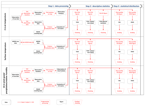
Following the proposed framework, we designed a guideline (Sect. S4 of the Supplement) and a workflow (Fig. 1) in the practice of model evaluation.

Figure 1 The workflow for model evaluation.

2.3 Observation datasets and modelled variables for model evaluation

In the existing literature, numerical weather prediction (NWP) models are typically evaluated by comparing the spatiotemporal patterns of the modelled variables with those of its corresponding near-surface observations. Moreover, we selected seven meteorological variables for the comparison, including 2 m air temperature, surface temperature, 10 m wind at u direction, 10 m wind at v direction, accumulated total cumulus precipitation, accumulated total grid precipitation, and 2 m relative humidity. These variables are the critical variables in the prognostic and diagnostic equations in the NWP model.

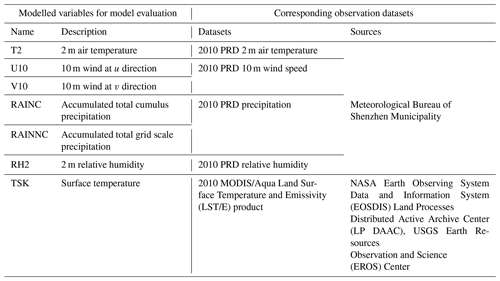
Table 2 lists the modelled variables and their corresponding observations in the model evaluation. The observation datasets are the point data except for the Moderate Resolution Imaging Spectroradiometer (MODIS) dataset, which is the grid data. All the modelled variables are grid data. The comparisons between modelled variables and their corresponding observed ones are comparisons between the grid value of the modelled variable and the point value matched to geographical locations, except for the comparison between the modelled surface temperature (TSK) and its corresponding observation retrieved from MODIS imagery. Moreover, the MODIS land surface temperature is the result of an inverse calculation based on longwave radiation through the atmosphere received by satellite according to the theory of blackbody. The MODIS land surface temperature is the manifestation of the surface synthetic radiation brightness temperature. Furthermore, in the land surface process, TSK is calculated iteratively according to the energy balance which involves longwave radiation, shortwave radiation, sensible heat, and latent heat, and accordingly, the final TSK value is also a manifestation of the surface synthetic radiation brightness temperature. Although there are some differences between TSK and the brightness temperatures observed by satellites, they describe relatively similar physical quantities. Therefore, we use TSK to compare with the MODIS land surface temperature.

Table 2 Modelled variables for model evaluation.

3 Technical preparation

3.1 Model setup

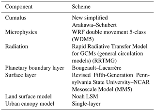
A telescoping nest's structure with four nested domains which are centred at 22^∘39^′30^′′ N, 114^∘11^′30^′′ E was set up as the horizontal domain baseline configuration in this study. Moreover, the same set of eta levels with 51 members was used in each horizontal domain. Furthermore, there were some physics components in the model, and each component had some different schemes for choosing. Table 3 shows the scheme chosen for each component. For more details, please refer to Sect. S4 of the Supplement.

Table 3 Schemes of the physics components.

3.2 Data preparation

Firstly, the 2010 National Centers for Environmental Prediction (NCEP) FNL (Final) Operational Global Analysis dataset (1^∘ grid spatial resolution and 6-hourly temporal resolution) was used as the gridded data in this study. Secondly, the geographical input data of the completed dataset of the WRF Preprocessing System (WPS) were used as the static geographical dataset in this study. Thirdly, the 2010 Pearl River Delta (PRD) urban land surface dataset, whose major sets of data include the land cover, vegetation coverage, urban morphology, and anthropogenic heat, was used. This was specially developed for refining the WRF primary data.

3.3 Primary data processing

Firstly, the primary data included the interpolated geodata files, the intermediate format meteorological data files, the horizontally interpolated meteorological data files, the initial condition data files, and the lateral boundary condition data files. Secondly, two primary data processing software packages (the geo_data_refinement processing package and wrf_input_refinement processing package) were developed for extracting the urban land surface attributes from the 2010 PRD urban land surface dataset and revising the corresponding fields of the related primary data files with these attributes.

Figure 2 Comparison of modelled and observed 2 m air temperature at 02:00, 08:00, 14:00, and 20:00.

Figure 3 Diurnal variation of 2 m air temperature.

4 Model evaluation

4.1 Evaluation of the 2 m air temperature

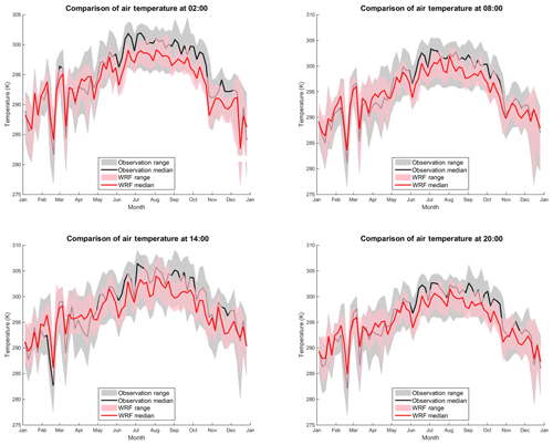
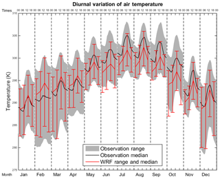
Using descriptive statistics, Fig. 2 compares the range and median values of the observed and the modelled 2 m air temperature at 02:00, 08:00, 14:00, and 20:00 in each month of the year. The modelled air temperatures always have similar spatiotemporal behaviour compared with the observed ones. Moreover, Fig. 3 compares the diurnal range and median of the observed and modelled air temperature each month of the year. Both the range and median of the 2 m modelled air temperature have the same diurnal variation as their corresponding observed ones in each month, although there are differences between the modelled and observed ones. Furthermore, as shown in Figs. 4 and 5, the modelled air temperatures have the same urban climatological spatial pattern as the observed ones in which the air temperature is higher in the urban areas than in non-urban areas irrespective of the time at which it is measured.

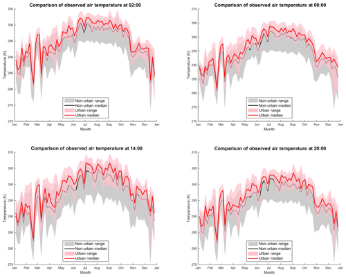
Figure 4 Comparison of observed air temperatures (at 02:00, 08:00, 14:00, and 20:00) in urban and non-urban areas.

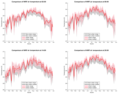
Figure 5 Comparison of modelled air temperatures (at 02:00, 08:00, 14:00, and 20:00) in the urban and non-urban areas.

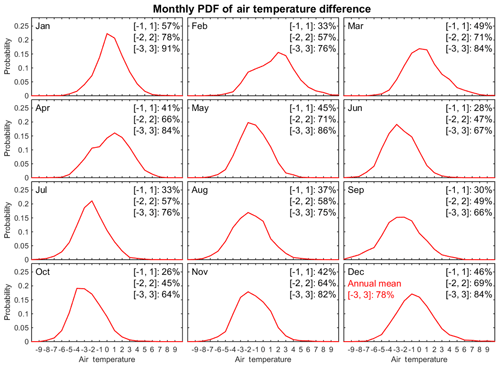
Using PSS to compare the statistical distribution of the observed and modelled air temperature, the model produces quite a good simulation of 2 m air temperature with an annual mean PSS of 0.724. Figure 6 shows that the monthly PSS of 2 m air temperature ranges from a minimum of 0.595 in July to a maximum of 0.886 in January and has an annual mean value of 0.724. This demonstrates that the model captured the PDF for the observed air temperature at least about 60 % in a month and over 72 % in a year. Figure 7 shows the PDF of differences between each value of each month's time series of modelled grid air temperatures and its corresponding observed ones. The probability of 3 ^∘C bias interval (the absolute value of the difference between modelled surface temperature and its corresponding observed one is 3 ^∘C) in a month varies from 64 % to 91 % and has an annual mean probability of this interval of 78 %.

Figure 6 Monthly PSS of the 2 m air temperature.

Figure 7 Monthly PDF of the 2 m air temperature difference.

In Fig. 6, the modelled distribution shifts to low temperatures in the period of June to October (summertime in the research area). Figure 7 shows that the differences between the modelled 2 m air temperatures and their corresponding observed ones exist the whole year. In fact, the difference includes not only the modelling bias but also an essential difference between a 1 km grid spatial average value and a value of a point located in this grid. Moreover, the observation is always located in an open area, and thus, the observed 2 m air temperature is the temperature of a point in the open area. The modelled 2 m air temperature is the mean temperature of a 1 km grid which always includes some vegetation-covered areas. In the summertime, the point air temperature in the open area without tree coverage is always higher than its corresponding mean air temperature of a 1 km grid with some vegetation coverage.

To sum up, the model produces quite a good simulation of 2 m air temperature with an annual mean PSS of 0.724. It also captures the behaviours of monthly and diurnal variation of observed 2 m air temperatures. Moreover, the modelled air temperatures have the same urban climatological patterns as those of the observed ones.

4.2 Evaluation of surface temperature

For descriptive statistics, the modelled surface temperatures have the same annual variations as those of the MODIS ones. Moreover, both the modelled surface temperatures and their corresponding observations from MODIS also have the same urban climatological patterns; that is, urban areas have higher surface temperatures than non-urban areas during the entire day. For more details, please refer to Figs. S6, S7, and S8 in the Supplement.

Regarding the statistical distribution, the modelled 02:00 and 14:00 surface temperatures represent the corresponding MODIS ones with an acceptable PSS. The monthly PSS of modelled surface temperatures ranges from 0.629 to 0.794 at 02:00 and from 0.479 to 0.777 for modelled at 14:00 respectively. The annual mean PSS of modelled surface temperatures at 02:00 and 14:00 is 0.702 and 0.623 respectively. Accordingly, both modelled surface temperatures at 02:00 and 14:00 are quite a good fit in MODIS surface temperature with a PSS of over 0.6. Moreover, the monthly probabilities of a 3 ^∘C bias interval (the absolute value of the difference between modelled surface temperature and its corresponding MODIS one is 3 ^∘C) at 02:00 range between 69 % and 98 % and have quite a high annual mean value of 87 %. The probabilities of a 3 ^∘C bias interval at 14:00 range from 54 % to 84 % and have a high annual mean value of 73 %. For more details, please refer to Figs. S9, S10, S11 and S12.

However, we also observed noticeable differences between the modelled surface temperature and its corresponding MODIS one in some grids. An analysis which was conducted on the MYD11A1 dataset finds that there are many grids whose quality was not evaluated in the MYD11A1 dataset, and accordingly, it is highly possible that this difference includes an observation bias. Moreover, due to the difference between the temporal coverages of the model outcome and its corresponding observation from MODIS, the observed difference also includes a bias introduced by the difference in measured time. Furthermore, the resampling operation on the MODIS dataset also causes a technical bias in some grids.

To sum up, the modelled 02:00 and 14:00 surface temperatures represent the corresponding MODIS ones with an acceptable PSS. Moreover, the modelled surface temperatures also have the same annual variations and the same urban climatological spatial patterns as that of those MODIS ones.

4.3 Evaluation of the 10 m wind speed

Using descriptive statistics, we compared the range and median values of the observed and the modelled 10 m wind speeds at 08:00, 14:00, 20:00, and 02:00 in each month of the year. The modelled 10 m wind speed always has a similar behaviour of spatiotemporal variation with the observed ones. Moreover, the modelled 10 m wind speed also has the same urban climatological spatial pattern as the observed ones in which the 10 m wind speed is lower in the urban areas than in non-urban areas, irrespective of the time at which it is measured. For more details, please refer to Figs. S13, S14, and S15.

From the point of view of the statistical distribution, the monthly PSS of the modelled 10 m wind speed ranges between 0.482 and 0.802 and has an annual mean value of 0.660. Moreover, the monthly probabilities of the 3 m s⁻¹ bias interval (the absolute value of the difference between modelled wind speed and its corresponding observed one is 3 m s⁻¹) range between 61 % and 83 %. For more details, please refer to Figs. S16 and S17.

We also observed the deviation which the modelled distribution shifts to high speed. The difference in the speed of the modelled 10 m wind and its corresponding observed one is not entirely caused by the model bias. The observation altitude of the modelled 10 m wind is different from its corresponding observed one. The modelled outcomes measure the upper air movement of the urban canopy, but the observations measure the air movement inside the canopy. The locations of modelled and observed air movements concerning the canopy would cause an essential difference between the modelled and observed values. Moreover, this difference also includes an essential difference between a 1 km grid spatial average value and a value of a point located in this grid.

Demonstrated by comparisons, the modelled ones of 10 m wind speed also have the same annual variation and the same urban climatological spatial pattern as that of the observed ones. The model also simulates 10 m wind speed with acceptable PSS and accuracy.

4.4 Evaluation of precipitation

From descriptive statistics, the modelled precipitations always have similar behaviour of spatiotemporal variation compared with the observed ones. For more details, please refer to Figs. S18, S19, and S20.

Demonstrated by the statistical distribution, the monthly PSS of modelled precipitation ranges between 0.444 and 0.747 and has an annual mean value of 0.579. Moreover, the model simulated precipitation with an accuracy in which the monthly probabilities of the 3 mm bias interval (the absolute value of the difference between modelled precipitation and its observed one is 3 mm) range between 39 % and 89 % and have an acceptable annual mean value of 67 %. For more details, please refer to Figs. S21 and S22.

However, the probability of 3 mm bias intervals is quite low in some months; for example, the one was 39 %, 50 %, and 53 % in June, September, and May respectively. The modelled precipitations deviated from their corresponding observed ones in these 3 months.

To sum up, the modelled precipitations also have the same annual variation as those of the observed ones. Moreover, the comparison of experiments and observations concerning the modelled and observed measurements of precipitation provide evidence that the model simulates precipitation with an acceptable PSS and accuracy.

4.5 Evaluation of relative humidity

We compared the range and median values of the observed and modelled relative humidity values across the spatial extent of the interested area stratified by time of day (08:00, 14:00, 20:00, and 02:00) and month. It is apparent that the modelled values always have similar behaviour in spatiotemporal variation with the observed ones, although all modelled median values are higher than the corresponding observed ones. Moreover, the modelled relative humidity has a similar spatial pattern compared with the observed one in which the relative humidity is lower in the urban areas than in the non-urban areas for all times of day and months. For more details, please refer to Figs. S23, S24, and S25.

Demonstrated by the statistical distribution, the monthly PSS of the modelled relative humidity ranges between 0.525 and 0.786 and has an annual mean value of 0.673. Moreover, the model simulates the relative humidity with quite good accuracy in which the monthly probabilities of the 20 % bias interval (the absolute value of the difference between modelled precipitation and its observed one is 20 %) range between 77 % and 96 % and have a high annual mean value of 91 %. For more details, please refer to Figs. S26 and S27.

To sum up, the model simulates the relative humidity with acceptable PSS and accuracy. Moreover, it also stimulates the monthly variation and urban climatological spatial patterns of relative humidity appropriately.

5 Discussion and conclusions

5.1 Model evaluation using observations

We need more practical model evaluation methods for better comparisons between model outcomes and observations to serve as partial support for the reliability of urban climate simulations and any conclusions based on the simulation results. The atmospheric model also is one of the earth science numerical models. An earth science model can simulate a resonance with the natural system (Oreskes et al., 1994), and accordingly, a climate simulation should aim at modelling the temporal and spatial meteorological features of climate. Therefore, a model evaluation should aim at assessing the similarity of temporal and spatial features between the modelled results and observations. In this study, the PSS was used for assessing the similarity quantitatively, and the graphic of a temporal comparison of spatial variation was used for assessing the similarity qualitatively. The quality of simulation was evaluated by using both descriptive statistics, such as the annual mean accuracy, and statistical distributions, such as the PSS metric. Similar spatial and temporal behaviours between the modelled variables and their corresponding observations are also illustrated.

Utilizing the proposed model evaluation methods, evaluation results in this case study indicate that this atmospheric model appropriately portrayed the annual variations in the climatological patterns of air temperature, surface temperature, 10 m wind speed, and air relative humidity. We observe that the simulation model captured similar temporal and spatial meteorological features of urban climate. From a quantitative perspective, the model achieved at least an acceptable PSS and accuracy in the simulations of 2 m air temperature, surface temperature, 10 m wind speed, precipitation, and air relative humidity, which means that the simulation results are acceptable approximations of the observations. Apparently, according to the above evaluations, the proposed simulation model in our case study is sufficiently reliable in reproducing meteorological features of urban climate at a 1 km spatial resolution.

The good match, in our study or any other study, between the model outcomes and observations can only support that the simulation results are acceptable approximations of the observations in the specific spatiotemporal coverages in respective studies. These comparisons are inadequate for model “verification” or “validation”. Returning to the philosophical basis, the terms verification and validation imply the confirmation of truth and legitimacy respectively (Oreskes et al., 1994). We get observations of meteorological characters from monitoring stations, and that is why the observations come in points and suffer from frequent missing data. Therefore, it is common that the spatiotemporal coverage of the observations can only partially match that of the modelling outcomes, which can be proved by the model evaluation process regarding air temperature, surface temperature, and other factors mentioned above. A good match between a model outcome and its corresponding observation at specific locations is no guarantee of a good match at other locations. Similarly, a good match between the model outcomes and the corresponding observations for a historical period is no guarantee of a good match in the future. Moreover, a good match between the model outcomes and corresponding observations for a limited spatiotemporal range does not guarantee that the model is free from initial and model uncertainties. Consequently, even a complete match between the observations and model outcomes does not ensure a successful verification and validation of the modelling system, let alone an incomplete match in practice (Oreskes et al., 1994). Theoretically, verifying or validating an atmospheric model is impossible. However, an earth science model can represent a natural system accurately to some extent (Oreskes et al., 1994), so it is feasible to evaluate atmospheric model outcomes with the observation data using practical spatial and temporal comparisons, which seems to be the best way possible to evaluate the performance of an atmospheric model. Nevertheless, we should always be aware of imperfectness.

5.2 The essential difference, observation bias, and model bias

Observations are probably the best reference we get to evaluate the simulation results, but that does not mean observations are perfect for such an evaluation. The comparison between the model outcome and observations alone cannot make a complete model evaluation, since it does not rule out the essential difference, observation bias, and model bias.

The essential difference refers to the fact that model outcomes from the simulation models are average values of a grid, while the observations are point-based, which only measure the meteorological conditions around the location of the monitoring station. Comparing the average value within a spatial area, the size of which ranges from 0.25 to over 100 km², with point-based observations is problematic for two main reasons. (1) The average value in a grid is calculated under the assumption that the grid is homogeneous, which is usually not true especially when detailed urban morphology is considered, and so the average value is usually lower than that of point-based observations. (2) Point-based observations are likely to be significantly affected by the surrounding environment of the monitoring site, lacking representativeness of the meteorological condition in the area. Therefore, the comparison between modelled outcomes and observations is biased, although it is usually the only model evaluation approach we get so far. The only exception is using the observations from remotely sensed imagery; for example, we used the land surface temperature product from MODIS/Aqua to evaluate the modelled temperature of the surface skin. However, there are many grids whose quality has not been evaluated in the MODIS/Aqua Land Surface Temperature product, and accordingly, the difference between the modelled temperature of the surface skin of a grid and its corresponding one in the MODIS/Aqua Land Surface Temperature product possibly includes an observation bias.

The model bias refers to the uncertainty caused by differences between the actual atmospheric physical processes and the approximations in the model (Skamarock et al., 2005, 2008). The fine-scale details are constructed by a limited area atmospheric model which consists of physical components driven by the lateral boundary conditions of coarse-scale meteorological data and land surface forcing data (Lo et al., 2008; Hong and Kanamitsu, 2014). However, these details do not exist in the coarse-scale meteorological data (Hong and Kanamitsu, 2014). A limited area atmospheric model can represent a natural atmospheric system accurately to some extent rather than entirely. The simulation models are supposed to include many more complex atmospheric physical processes to explain meteorological states with high spatial and temporal resolutions, but many of them have to be omitted or empirically approximated due to limitations in knowledge and computational efficiency. Given the complexity of simulation models, estimating error propagation in these models is complicated, and thus model evaluation becomes the only quality control of simulation results, especially for high-resolution urban climate simulations which are more sensitive to the inadequacies of the atmospheric model, inappropriate configuration of the modelling system (Warner, 2011), and the quality of input data.

5.3 Conclusions

Following the proposed framework, we first measured both the descriptive statistics of each pair of the modelled and observed meteorological variables and the difference between them at each spatiotemporal epoch. Secondly, we respectively analysed the probability density function of modelled and observed meteorological variables, and the probability of the difference values between them. With visualized PDFs, we can understand the empirical distribution of the simulation bias and notice outliers directly, which may shed light on the calibrations of further models' results. Thirdly, we apply the analysis using descriptive statistics and statistical distributions to the other temporal scales: monthly and time of day. By doing so, we further investigate temporal variations in different months of the year and times of the day.

In conclusion, we emphasize in this paper that model evaluation is necessary and usually the only process that guarantees the reliability of simulation outcomes, and so utilizing a practical model evaluation process to reach an acceptable agreement between the simulated and observed meteorological variables should be the premise of any conclusion drawn from the modelling results. The emerging high-resolution urban climate simulation models are especially sensitive to possible initial and model uncertainties. In this vein, we proposed a practical methodological framework for urban climate model evaluation that examines not only the matches between the spatiotemporal patterns of the modelled and observed variables but also the statistical distribution of the difference between the modelled variables and their corresponding observations. Moreover, the proposed method utilized PSS to statistically quantify the extent of overlap between the PDFs of modelled variables and their corresponding observations, which, we argue, was a more informative and useful indicator for the quality of modelling outcomes compared to existing metrics such as residuals and correlations. By doing so, we hope to provide more capable tools that improve the quality control in future research using numerical meteorological simulations, especially high-resolution urban climate simulations.

We also intend to raise awareness and attention over model evaluation methods within the modelling community, since new findings without sophisticated understanding, control of model uncertainties, and systematic assessments of model outcomes may be scientifically misleading. Moreover, we reminded the modeller that they should be cautious about concluding a quantitative finding because it is impossible to identify the essential difference, observation bias, and model bias in the difference between observations and their corresponding modelled values. Furthermore, although this methodological framework of model evaluation was designed for urban climate simulation, it can also be applied in local-scale climate simulation in urban or non-urban regions.

At the spatial dimension, the climate areas were classified into the different scales, such as local (less than 10⁴ km²), regional (from 10⁴ to 10⁷ km²), and global (greater than 10⁷ km²) scales (Intergovernmental Panel on Climate Change, 2012). The similarity between the spatial patterns of the modelled and observed variables is indeed a significant component in model evaluation of regional and global climate, especially regarding the spatial difference of the precipitation belt and atmospheric circulation. In the previous literature, there were not many papers on the methods of spatial pattern comparison for local climate simulation, which is a research gap for future exploration.

Finally, some future research ideas were inspired. The effects of the selected physical components on the evaluated modelling accuracy are not clear, which requires further control experiments. Also, the effects of the refined urban land surface datasets on the evaluated modelling accuracy also require further discussion.