the Creative Commons Attribution 3.0 License.
the Creative Commons Attribution 3.0 License.
Description and evaluation of the Diat-HadOCC model v1.0: the ocean biogeochemical component of HadGEM2-ES
Ian J. Totterdell
The Diat-HadOCC model (version 1.0) is presented. A simple marine ecosystem model with coupled equations representing the marine carbon cycle, it formed the ocean biogeochemistry sub-model in the Met Office's HadGEM2-ES Earth system model. The equations are presented and described in full, along with the underlying assumptions, and particular attention is given to how they were implemented for the CMIP5 simulations. Results from the CMIP5 historical simulation (particularly those for the simulated 1990s) are shown and compared to data: dissolved nutrients and dissolved inorganic carbon, as well as biological components, productivity and fluxes. Where possible, the amplitude and phase of the predicted seasonal cycle are evaluated. Since the model was developed to explore and predict the effects of climate change on the marine ecosystem and marine carbon cycle, the response of the model to the RCP8.5 future scenario is also shown. While the model simulates the historical and current global annual mean air–sea CO2 flux well and is consistent with other modelling studies about how that flux will change under future scenarios, several of the ecosystem metrics are less well simulated. The total chlorophyll is higher than observations, while the primary productivity is just below the estimated range. In the CMIP5 simulations certain parameter choices meant that the diatoms and the misc-phytoplankton state variables behave more similarly than they should, and the surface dissolved silicate concentration drifts to excessively high levels. The main structural problem with the model is shown to be the iron sub-model.
- Article
(37891 KB) - Full-text XML
- BibTeX
- EndNote


The works published in this journal are distributed under the Creative Commons Attribution 4.0 License. This license does not affect the Crown copyright work, which is reusable under the Open Government Licence (OGL). The Creative Commons Attribution 4.0 License and the OGL are interoperable and do not conflict with, reduce or limit each other.
© Crown copyright 2019
The recent publication of the 5th Assessment Report of Working Group 1 of the Intergovernmental Panel on Climate Change (IPCC, 2013) includes an analysis of four possible future scenarios of how the global climate might change over the next few decades in response to anthropogenic emissions of carbon dioxide (CO2) and other anthropogenic influences (e.g. changes in land use). These future scenarios are informed by the results of the 5th Climate Model Intercomparison Project, CMIP5 (Taylor et al., 2012), for which 47 different climate models ran one or more of the scenarios. Models are of course an absolute necessity for predicting future climate, since no observations can exist.
The number of general circulation models (GCMs) available to study climate has increased rapidly in recent years, and the range of processes and feedbacks that they can represent has also become more comprehensive. Initially there were just physical models describing the circulation of the atmosphere and the ocean and how those circulations redistributed and stored heat, as well as the response of the system to rising atmospheric CO2. The first coupled climate model to include representations of the land and marine carbon cycles, including terrestrial vegetation and soils and marine ecosystems, capable of representing their basic feedbacks on the climate was HadCM3LC (Cox et al., 2000). In that model, the terrestrial vegetation was described by the TRIFFID model (Cox, 2001), while the chemistry of carbon dioxide in seawater and the marine ecosystem was described by the Hadley Centre Ocean Carbon Cycle (HadOCC) model (Palmer and Totterdell, 2001). The latter is a simple nutrient–phytoplankton–zooplankton–detritus (NPZD) model using nitrogen as the limiting element.
A brief overview of Met Office model nomenclature is useful here. The Met Office modelling system used (over a time period of several decades) for climate studies and for numerical weather prediction is known as the Unified Model, and the coupled climate models exist as various versions of it. The HadCM3LC model mentioned above featured a lower-resolution (“L”) ocean sub-model than the HadCM3C model, which itself was the member of the HadCM3 family of coupled climate models (Gordon et al., 2000; version 4.5 of the Unified Model) that featured an interactive carbon cycle (“C”) in the atmosphere, on land and in the ocean. The HadGEM2 family of climate models (The HadGEM2 Development Team, 2011), a development of HadCM3 with enhanced resolution and improved parameterisations that was used for CMIP5 simulations, was version 6.6 of the Unified Model. In particular, HadGEM2-ES (Collins et al., 2011), featuring active Earth system components including version 1.0 of the Diat-HadOCC sub-model, was version 6.6.3.
The aim of this paper is to describe and validate version 1.0 of the Diat-HadOCC model, as used in HadGEM2-ES to run simulations for the CMIP5 experiment. Although the simulations were run several years ago this description of the model is important as a record and can inform other modellers of potential parameterisations that succeeded (or not) here. The equations are presented and described in detail, and reasons are given for certain choices made in the representation of processes and in the values of parameters. Where potential other uses of the model (e.g. in ocean-only simulations forced by reanalysis fluxes) differ from its use here, this is mentioned. The publicly available model output submitted to CMIP5 is used to evaluate the model, and its successes and weaknesses are discussed.
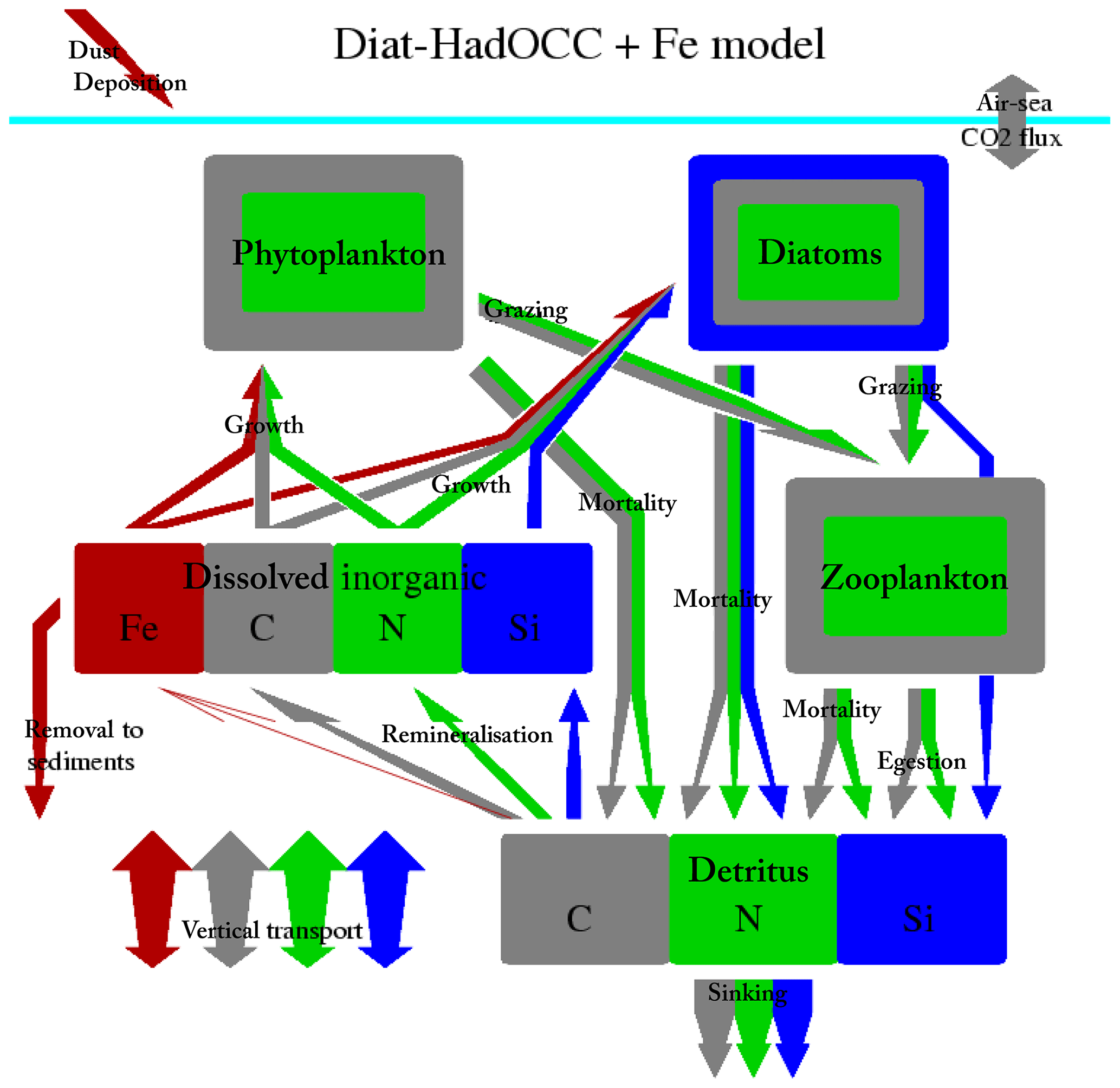
Figure 1Diagram of the Diat-HadOCC model components and flows of nitrogen, carbon, silicon and iron.
As shown in Table 1 and Fig. 1 the Diat-HadOCC model has 13 biogeochemical state variables representing three dissolved nutrients (nitrate, silicate and iron), two phytoplankton (diatoms and misc-phyto; plus diatom silicate), one zooplankton, three detritus compartments (detrital nitrogen, carbon and silicon), dissolved oxygen, dissolved inorganic carbon and alkalinity. “Misc-phyto(plankton)” refers to the “miscellaneous phytoplankton” term used in the CMIP5 database, i.e. any phytoplankton that is not specified to be a particular functional type. All the state variables are advected by the ocean currents and mixed by physical processes such as isopycnal diffusion, diapycnal diffusion and convective mixing. The biogeochemical processes that affect the biogeochemical state variables are shown below in basic form, with greater detail on the processes given in subsequent paragraphs. In the following equations all flows are body (point) processes except those in square brackets, which are biogeochemical flows across layer interfaces.
The terms in Eq. (1) show that the concentration of dissolved inorganic nitrogen is increased by the following (in order): a release of nitrogen associated with respiration by misc-phytoplankton (to keep the cell's molecular C:N ratio constant; Eq. 37); a corresponding release associated with diatom respiration (Eq. 36); fractions of the nitrogen released by the natural mortalities of misc-phytoplankton and of diatoms (the rest of the nitrogen in each case passes to sinking detritus DtN; see Eqs. 40 and 38); a release of nitrogen due to grazing by zooplankton on misc-phytoplankton, diatoms and detritus (Eq. 34); losses from zooplankton (mainly associated with respiration; Eq. 41); a fraction of the loss due to zooplankton mortality (natural and due to unmodelled grazing by higher trophic levels; Eq. 42); and nitrogen returned to the dissolved state by the remineralisation of sinking detritus in the water column (Eq. 46) and at the sea floor (Eq. 51). Conversely, the final two terms show that the concentration is decreased by uptake by misc-phytoplankton and diatoms to fuel photosynthesis and primary production (Eqs. A16 and A17, respectively). The processes of nitrogen deposition from the atmosphere, inflow from rivers and estuaries, release from sediments, nitrogen fixation, and denitrification are not included in the Diat-HadOCC model.
Equation (2) shows that the concentration of dissolved silicate is increased by the dissolution of detrital silicate in the water column (Eq. 48) and at the sea floor (Eq. 51), while it is decreased by uptake by diatoms to produce opaline shells in association with growth (Eq. A17; the Si:N ratio is a function of the dissolved iron concentration following Eq. 9). As with DIN, there are no inputs or losses of Si from or to the atmosphere, rivers, estuaries or sediments.
Each of the processes increasing or decreasing the dissolved inorganic nitrogen concentration has a counterpart that increases or decreases the dissolved inorganic carbon concentration; Eq. (3) shows those processes and also the two processes that affect DIC, namely the formation and dissolution of solid calcium carbonate (crbnt; Eq. 63) and the air–sea flux of CO2 (Eq. C1). Apart from the air–sea flux of CO2 there are no other inputs or losses of inorganic carbon to the ocean.
In this model, biologically mediated changes to the total alkalinity (which has units of millimolar equivalents per cubic metre). are associated with either the formation and dissolution of solid calcium carbonate or the uptake and release of dissolved inorganic nitrogen; Eq. (4) shows how these processes are related to the alkalinity. Because the carbonate ion has two charges the change in the alkalinity due to crbnt is double the change in DIC and of opposite sign. Although uptake by phytoplankton of dissolved nitrate does not directly change the alkalinity, it is usually associated with a balancing release of OH− ions, which does change it (Goldman and Brewer, 1980). In the model all the DIN taken up is assumed to be nitrate, but in the real ocean some of the nutrient will be dissolved ammonia, , which is associated with a release of H+ ions that change the alkalinity in the opposite sense to the OH− ions; the model's omission of ammonium ions is not a great problem as any that is taken up for growth will likely have been produced locally shortly before, given that ammonium has a short residence time in the upper water column.
Dissolved oxygen is included in the model as a diagnostic tracer: its concentration is changed by biological processes (as well as physical and chemical ones) but does not affect any other model state variable. It has particular value as a diagnostic of the respiration of organic matter at depth in the water column, but it also allows for the simulation of oxygen minimum zones and their evolution under climate change. It is assumed for the model that all respiration of organic matter is aerobic, so the same O:C ratio can be used for all ecosystem processes, including both uptake and release of O2; the second term in Eq. (5) (i.e. within the large brackets) connects such oxygen fluxes to those of organic carbon. The first term in that equation relates to the air–sea flux of oxygen. The third term, resetO2, is included to prevent the dissolved oxygen concentration from going negative: at the end of each time step, if the combination of physical fluxes and biological processes has taken the concentration in any grid cell below zero, the concentration is reset to zero and the amount that has been added to the model recorded. The column inventory of such reset additions is calculated and subtracted from the surface layer; because that layer is in close contact with the atmosphere this adjustment should never reduce the surface concentration to zero (and in the CMIP5 simulations never came close to doing so anywhere). This approach was adopted in the model to prevent negative concentrations of dissolved O2 while conserving the global O2 inventory.
2.1 Diatoms and misc-phytoplankton
In the model misc-phytoplankton and diatoms are both quantified by their nitrogen content and have units of millimoles of nitrogen per cubic metre (mMol N m−3). Their carbon contents are related to their nitrogen contents by fixed elemental ratios of and , respectively. Equation (6) shows that, in terms of biological processes, the misc-phytoplankton concentration is increased by growth and decreased by respiration, mortality and grazing by zooplankton. Equation (7) shows that the diatom concentration is increased and decreased by analogous biological processes but is additionally subject to sinking at a constant velocity VDm because of gravity. Equation (8) describes the (analogous) biological processes that increase or decrease the concentration of opal shells attached to living diatoms (diatom silicate), which is also subject to sinking (at velocity VDm); since the ratio of silicon in the diatom shell to nitrogen in the organic tissue of the diatom cell can vary, diatom silicate has to be represented as a distinct model state variable.
The growth of diatoms and misc-phytoplankton (dmPP and phPP, respectively) is a function of the availability of macronutrients and micronutrients, the temperature, and the availability of light. The growth limitation by dissolved nitrate (and, in the case of diatoms, also by dissolved silicate) in the model has a hyperbolic form, while that by dissolved iron is represented in a different way. The effect of dissolved iron (FeT) in the Diat-HadOCC model is to vary certain parameter values: the assimilation numbers (maximum growth rates) for diatoms and misc-phytoplankton ( and , respectively), the silicon:nitrogen ratio for diatoms , the zooplankton base preference for feeding on diatoms bprfDm and the zooplankton mortality . (Note that, because the base feeding preferences are subsequently normalised so that their sum is 1, changing the preference for diatoms will mean the preferences for misc-phytoplankton and for detritus also change.) The dependence of zooplankton parameters on the dissolved iron concentration is not intended to suggest a direct causal relation (or that the parameters relating to any single species of zooplankton are iron dependent) but rather reflect a change in the types and species of zooplankton that dominate the ecosystem when their phytoplankton prey species respond to greater iron stress by becoming more silicified; larger phytoplankton cells with thicker and more protective shells will be less palatable to predators and predated by larger mesozooplankton and macrozooplankton species, multi-cellular, and with different life cycles and lower specific mortality. Since there is only one zooplankton compartment in the Diat-HadOCC model its parameters must change to accurately represent such a shift. The parameterisation used here is based on the results of earlier, but unpublished, 1-D modelling work by the late Michael J. R. Fasham (personal communication, 2003), an extension of the work described in Fasham et al. (2006). Each of the iron-dependent parameters has an iron-replete value (the standard) and an iron-deplete value, and the realised value at a given time and location will be
where kFeT is a scale factor for iron uptake. In the CMIP5 simulations run using HadGEM2-ES (with the Diat-HadOCC model as the ocean biogeochemical component) only the value of varied (i.e. the iron-replete and iron-deplete values of the other parameters were set equal).
The Diat-HadOCC model, as coded, includes an option for the growth rate to vary exponentially with temperature according to Eq. (1) of Eppley (1972) (normalised so that default rates occur at 20 ∘C). However, for the CMIP5 simulations run using HadGEM2-ES the temperature variation of phytoplankton growth rate was switched off and the default values were used (i.e. in the equation below fTemp was always equal to 1).
In the above equations the combined effect of the temperature and macronutrient concentrations is limited to a maximum factor of 1.0 to guard against excessively fast growth should the water temperature should become very high (when the temperature factor is switched on).
The light dependency of the growth rates of misc-phytoplankton and diatoms is calculated using an implementation of the scheme presented in Anderson (1993); it is described in detail in Appendix A. In addition, although prescribed constant carbon:chlorophyll ratios (with the value 40.0 mg C per milligram of chlorophyll for each phytoplankton type) were used in the CMIP5 simulations the option exists in the Diat-HadOCC model to calculate a variable ratio (similar to that used in conjunction with the HadOCC model in Ford et al., 2012), and this is described in Appendix B.
2.2 Zooplankton and grazing
Zooplankton biomass (quantified by its nitrogen content) is increased by grazing (of misc-phytoplankton, diatoms and detrital particles; see Eq. 30) and decreased by losses such as respiration (Eq. 41) and by density-dependent predation by the unmodelled higher trophic levels (Eq. 42).
The grazing function used in the Diat-HadOCC model differs from that used in the HadOCC model in that it uses a “switching” grazer similar to that used in Fasham et al. (1990; hereafter FDM90). It is noted that some authors (e.g. Gentleman et al., 2003) recommend against using such a formulation because it can lead to reduced intake when food resources are increasing. The single zooplankton consumes diatoms, misc-phytoplankton and (organic) detrital particles. As in FDM90 the realised preference dprfX for each food type depends on that type's abundance and on the base preferences bprfX.
If MN and MC are the respective atomic weights of nitrogen and carbon (14.01 and 12.01 g mol−1) and is the Redfield C:N ratio (106 mol C : 16 mol N), then the terms convert from nitrogen or carbon units to biomass units that allow the various potential food items to be compared.
Note that the base preference values supplied (or calculated as a function of iron limitation) bprfX are normalised so that they sum up to 1. The available food is
and the grazing rates on the various model state variables are the following.
A fraction (1−fingst) of the grazed material is not ingested: of this, a fraction fmessy immediately returns to solution as DIN and DIC, while the rest becomes detritus. All of the grazed diatom silicate DmSi immediately becomes detrital silicate DtSi. Of the organic material that is ingested, a source-dependent fraction (βX) of the nitrogen and of the carbon is assimilable, while the remainder is egested from the zooplankton gut as detrital nitrogen DtN or carbon DtC. The amount of assimilable material that is actually assimilated by the zooplankton grzZp is governed by its C:N ratio compared to that of the zooplankton; as much as possible is assimilated, with the remainder immediately passed out as DIN or DIC.
2.3 Other processes
The other loss terms for diatoms, misc-phytoplankton and zooplankton are the following.
In the above equations phmin is a set (low) concentration of Ph below which the natural mortality of misc-phytoplankton is set to zero; the inclusion of this term was a pragmatic and necessary choice in an early version of the model to prevent the misc-phytoplankton from dying out in certain parts of the seasonal cycle at high latitudes (it was not found to be necessary to include a similar term for diatoms). It can be rationalised as representing the ability of phytoplankton to enter a “cyst” state under certain stressful conditions. Although respiration involves a release of carbon (as CO2) the fixed C:N ratios used in the models for misc-phytoplankton, diatoms and zooplankton require a balancing release of nitrogen from those model compartments. The “natural mortality” of both phytoplankton variables refers to cell death, particularly including that caused by viral infections, which will be density dependent. The zpmort refers primarily to zooplankton losses due to predation by unmodelled higher trophic levels and is the closure term of the modelled ecosystem.
2.3.1 Detrital sinking and remineralisation
All detrital material sinks at a constant speed VDt at all depths. Diatoms (and their associated silicate) sink at a constant speed VDm at all depths. Detrital remineralisation (of DtN and DtC) is depth dependent, the specific rate varying as the reciprocal of depth but with a maximum value. This functional form gives a depth variation of detritus consistent with the Martin et al. (1987) power-law curve. Dissolution of opal does not vary with depth.
Since there are no sediments in the Diat-HadOCC model, all detritus that sinks to the sea floor is instantly remineralised to N, C or Si and spread through the lowest three layers (above the sea floor). Spreading over the bottom three levels is a numerical artifice to prevent excessive build-up of high concentrations (below regions of high primary productivity and sinking detritus) in bathymetric canyons that are too narrow to support advection and so rely on weak vertical mixing to redistribute N, C or Si being introduced by the instant sea-floor remineralisation (such high concentrations would themselves be artefacts of the model). It is reasoned that where the ocean is (thousands of metres) deep the time required for dissolved inorganic nutrients and carbon to return to the euphotic zone will be dominated by the slow deep circulation and mixing, and shortening the path by at most a couple of levels will not significantly affect this time; on the shallow shelves the instant transport upwards through two levels will actually partially mitigate the absence from the model of tidal mixing, which is very important in such environments in the real ocean. Diatoms (and associated silicate) that sink to the sea floor instantly die and become DtN, DtC and DtSi, as appropriate, in the lowest layer. Therefore, if btmflxY is the value of [Ysink] at the sea floor,
where btmflxX is the sinking flux of X to the sea floor and ΔbMl is the combined thickness of the bottom M layers (of course, which layers those are will vary according to the location).
2.3.2 The iron cycle
Iron is added to the ocean by dust deposition from the atmosphere (prescribed or passed from the atmospheric sub-model in coupled mode; penultimate term in Eq. 53), with a constant proportion (by weight) of the dust being iron which immediately becomes part of the total dissolved iron pool FeT. Iron is taken up by diatoms and misc-phytoplankton during growth in a fixed ratio to the carbon taken up () and moves through the ecosystem in the same ratio, except that any flow of carbon to DtC is associated with a flow of iron back to solution, as there is no iron in organic detritus in the model. Since the iron sub-model was developed there have been many experimental and observational studies of the marine iron cycle (e.g. Boyd et al., 2017), which have shown that this assumption (it was a pragmatic decision to maintain adequate levels of dissolved iron in the euphotic zone) is a bad one; the performance of the iron model is discussed further in the Conclusions section.
While all iron that flows through the ecosystem is returned to solution, there is a final loss term for dissolved iron, namely (implicit) adsorption onto pelagic sinking mineral particles (not the model's detrital particles) and thence to the (implicit) sediments (last term in Eq. 53). Only the fraction of FeT that is not complexed to organic ligands can be adsorbed. The uncomplexed (free) iron concentration FeF and the complexed concentration FeL are found by assuming a constant uniform total ligand concentration LgT and a partition function KFeL; the adsorption flux feadsorp is derived from that.
In the above equations, LgF is the portion of the ligand concentration that is not bound to iron.
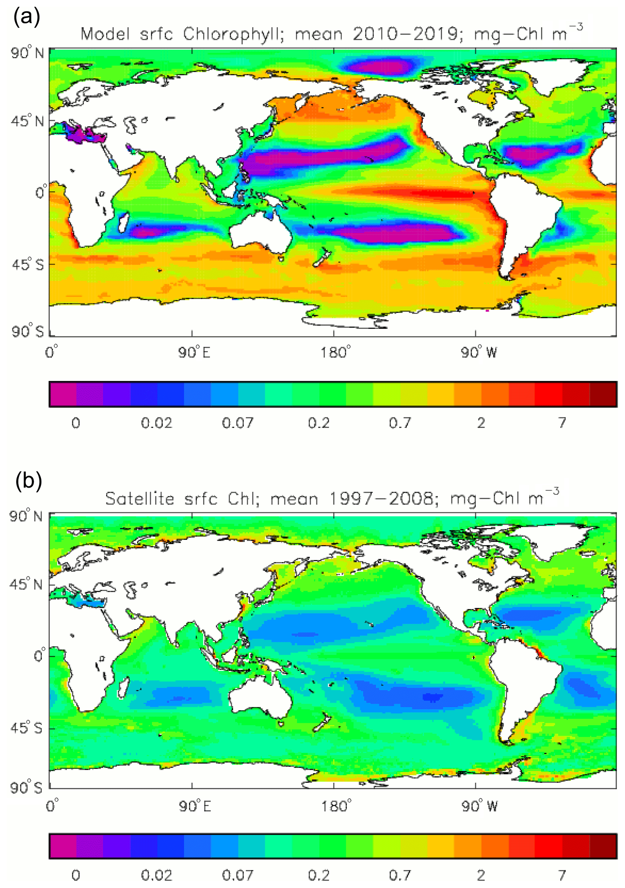
Figure 2Comparison of surface chlorophyll: (a) mean over the years 2010–2019 from the model, historical+RCP8.5 scenario; (b) mean over 1998–2007 from GlobColour, with further processing as described in Ford et al. (2012) (mg Chl m−3).
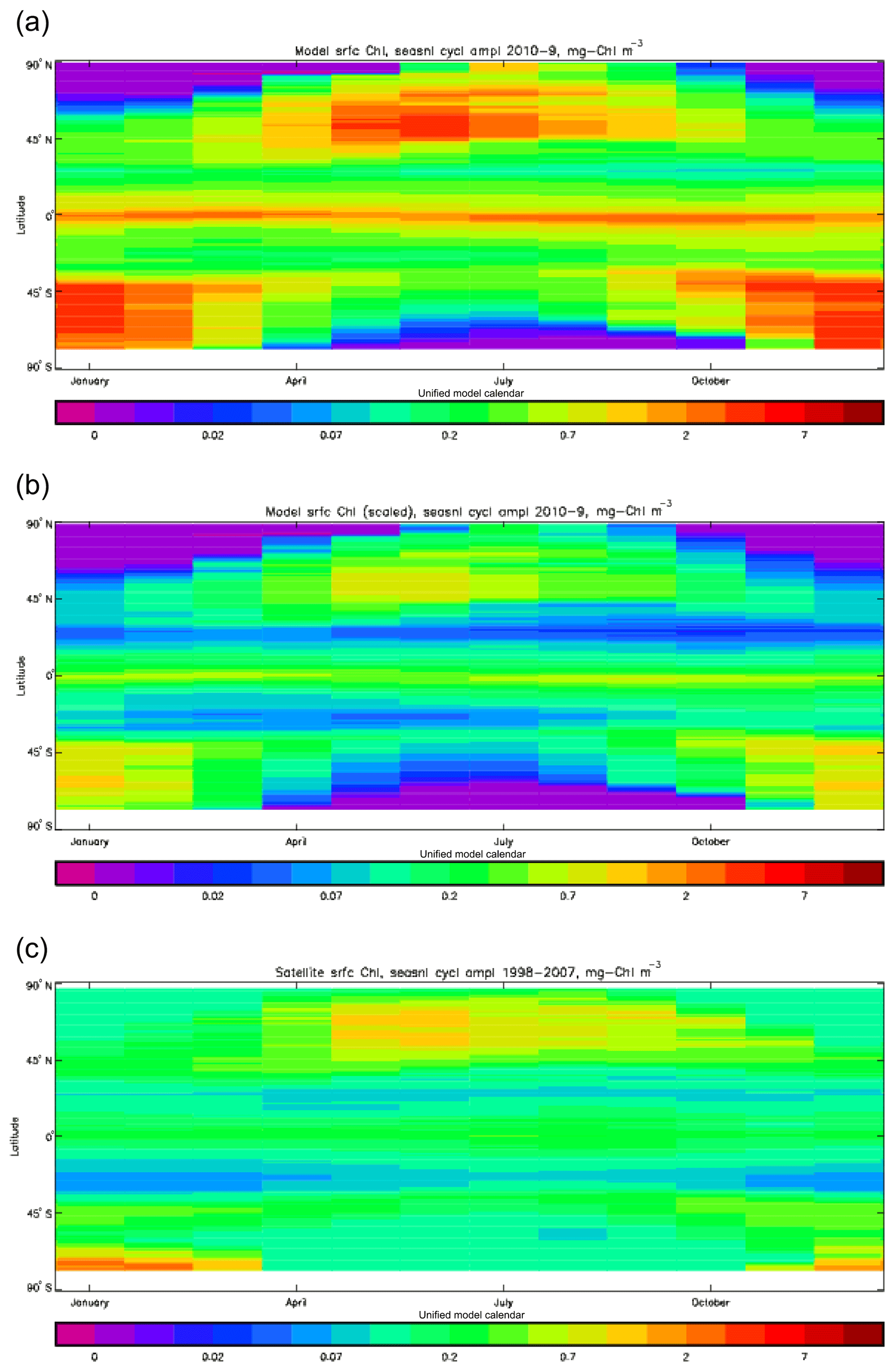
Figure 3Seasonal cycle of global zonal mean surface chlorophyll (mg Chl m−3): (a) average over the years 2010–2019 from the model, historical+RCP8.5 scenario; (b) the same but scaled by factor so that the model mean matches the observations; (c) satellite-derived data from GlobColour, averaged over 1998–2007.

Figure 4The amplitude (a, c; mg Chl m−3) and phase (b, d; units are “fraction of year”) of the seasonal cycle of surface chlorophyll in the model (a, b; average over years 2010–2019, historical+RCP8.5 scenario, amplitude scaled by factor of 0.213∕0.812) and in the GlobColour data (c, d; average over years 1998–2007). The amplitude has been determined by finding the best-fitting sine curve through the monthly mean values of the average cycle at each point, and the phase refers to the fraction of the year when the fitted curve is at its maximum. Points are left white if the variance of the residual (after the best-fitting sine curve has been removed) is more than half that of the original seasonal cycle.
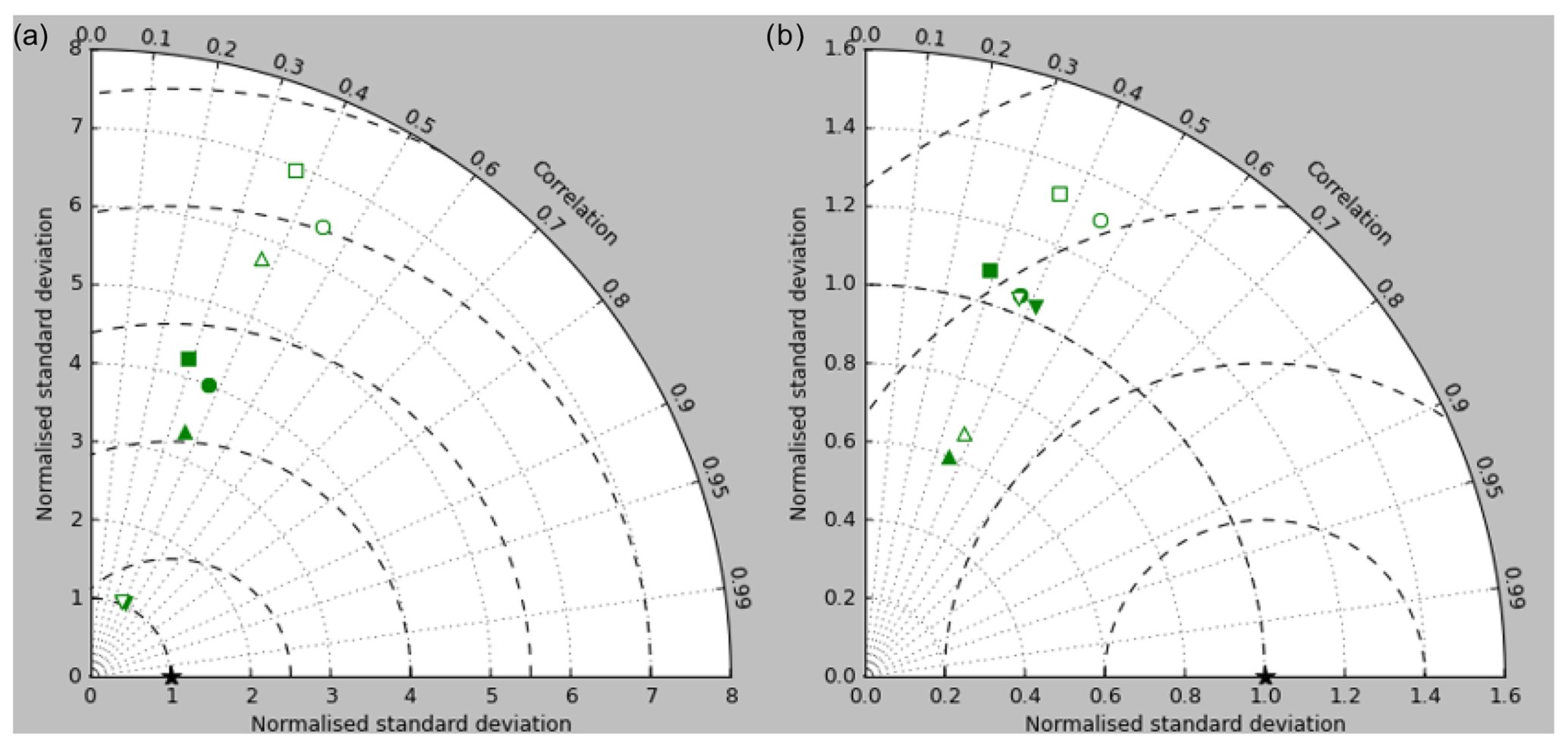
Figure 5Taylor diagrams of model surface chlorophyll compared to the GlobColour product. Solid symbols represent correlations and standard deviations from points in all parts of the ocean (except inland seas), while open symbols have had a mask applied to remove the Arctic Ocean and two grid boxes around the coast, as explained in the text. Squares represent the annual mean of all points, while circles, up-pointing triangles and down-pointing triangles respectively represent the midpoint, amplitude and phase of the sine curve that best fits the seasonal cycle (where the variance of the residual is less than half the variance of the cycle). The diagram in (a) uses the raw model results, while that in (b) uses the model chlorophyll scaled to give a comparable global mean to the observations (again as explained in the text).
2.3.3 The calcium carbonate sub-model
Solid calcium carbonate is implicitly produced in a constant ratio () to organic carbon produced by misc-phytoplankton. Note that this ratio is not the rain ratio, which compares the ratio of inorganic to organic carbon in the particulate sinking flux below the euphotic zone, since it compares the production of the respective carbon types, and while all the model inorganic carbon is exported from the surface layer only a fraction of the organic carbon is, and so this ratio represents the average of the product of the rain ratio and the organic export ratio. The total production (of solid calcium carbonate) is summed over the surface layers (those for which production is non-zero) and instantly redissolved equally through the water column below the (prescribed) lysocline. If the sea floor is shallower than the lysocline, then the dissolution takes place in the bottom layer (there being no sediments). The depth of the lysocline is always coincident with a layer interface and is constant both geographically and in time. In the following equations, ccfrmtn and ccdsltn are respectively the rate of formation and dissolution of solid calcium carbonate in a given layer, xprtcc is the export of calcium carbonate from the surface layers, and crbnt is the net flux of carbon from solid calcium carbonate to DIC:
where Δn is the thickness of layer n and Δdsl is the total thickness of the valid layers (where dissolution can occur) in that water column, which is equal to the distance between the lysocline and the sea floor if the lysocline is shallower than the sea floor and the thickness of the deepest layer otherwise.
2.3.4 Air–sea fluxes
Finally, the calculations of the air-to-sea fluxes of O2 and CO2 ([Oxyasf] and [CO2asf], respectively) follow the methodology of OCMIP. The flux is the product of the gas-specific gas transfer (piston) velocity Vp and the difference between the gas concentrations in the atmosphere (just above the sea surface), Xsat, and in the (surface) ocean, Xsurf:
The details can be found in Appendix C.
The Diat-HadOCC model formed the ocean biogeochemical component of the HadGEM2-ES Earth system model (Collins et al., 2011), which is part of the HadGEM2 family of coupled climate models (The HadGEM2 Development Team, 2011). Full details of the model set-up for the experiments described here can be found in those references, but a brief description is given here.
The atmospheric physical model has a horizontal resolution of 1.25∘ latitude by 1.875∘ longitude and a vertical resolution of 38 layers (to a height of 39 km). A time step of 30 min is used. Eight species of aerosol are included in the atmosphere, as is a representation of mineral dust (described in more detail below). The UK Chemistry and Aerosols (UKCA) model (O'Connor et al., 2014) describes the atmospheric chemistry. MOSES II (Essery et al., 2003) is used for the land-surface scheme, with additional processes and components as described in papers about the derived JULES scheme by Best et al. (2011) and Clark et al. (2011). The hydrology includes a river-routing sub-model based on the TRIP scheme (Oki and Sud, 1998), which supplies freshwater (but not nutrients, carbon or alkalinity) to the ocean. The TRIFFID dynamic vegetation model (Cox, 2001; Clark et al., 2011) and a four-pool implementation of the RothC soil carbon model (Coleman and Jenkinson, 1996, 1999) are used to represent the terrestrial carbon cycle. TRIFFID calculates the growth and phenology of five plant functional types (broadleaf trees, needle-leaf trees, C3 grasses, C4 grasses and shrubs) so that the (terrestrial) gross primary production (GPP), net primary production (NPP), and thereby also the terrestrial sources and sinks of atmospheric carbon can be determined.
The ocean physical model is based on that described in Johns et al. (2006), with developments as detailed in the paper by The HadGEM2 Development Team (2011). It has a longitudinal resolution of 1∘, while the latitudinal resolution is also 1∘ poleward of 30∘ (N or S) but increasing from that latitude to at the Equator. In the vertical there are 40 levels with thicknesses increasing monotonically from 10 m in the top 100 to 345 m at the bottom and with a full depth of 5500 m. A time step of 1 h is used. The computer code is based on that of Bryan (1969) and Cox (1984). The active ocean tracers (temperature and salinity) use a pseudo 4th-order advection scheme (Pacanowski and Griffies, 1998), while the passive tracers (including all the ocean biogeochemical tracers) use the UTOPIA scheme (Leonard et al., 1993) with a flux limiter. The Gent and McWilliams (1990) adiabatic mixing scheme is used in the skew flux form from Griffies (1998) and with a coefficient that varies spatially and temporally following Visbeck et al. (1997). An implicit linear free-surface scheme (Dukowicz and Smith, 1994) is included for freshwater fluxes. A simple upper mixed layer scheme (Kraus and Turner, 1967) is used for vertical mixing due to surface fluxes of heat and freshwater for both active and passive tracers. The sea-ice model is based on the Los Alamos National Laboratory sea-ice model, CICE (Hunke and Lipscomb, 2004), including five thickness categories, elastic–viscous–plastic ice dynamics (Hunke and Dukowicz, 1997) and ice ridging. The presence of sea ice of any thickness reduces to zero the light entering the water column (so preventing photosynthesis by marine phytoplankton) and completely blocks the transfer of gases between the atmosphere and ocean.
Coupling between the atmosphere and ocean models happens every 24 model hours. After 48 atmospheric time steps (of 30 min each) have been run the fluxes of heat, freshwater, wind stress and wind mixing energy, along with any necessary biogeochemical quantities, are determined (usually as a time mean over the 24 h) and passed via the coupler to the ocean. Because the atmosphere and ocean models use different grids this involves re-gridding, with special care needing to be taken at the coasts where an atmospheric grid box may correspond to both an ocean and a land grid box. The ocean is then run for 24 time steps (of 1 h each) and the relevant fluxes calculated and passed to the atmosphere.
The biogeochemical quantities passed from the atmosphere to the ocean are the deposition flux of mineral dust and the concentration of CO2 in the lowest atmospheric level, while the flux of CO2 and the flux of dimethyl sulfide (DMS) are passed from the ocean to the atmosphere. Note, however, that in the concentration-driven simulations for which the results are presented here the atmospheric CO2 concentration “seen” by the ocean is not passed from the atmosphere but prescribed in the ocean model (in such a way that it agrees with the atmospheric concentration prescribed in the atmosphere once the different units are taken into account), and while the flux of CO2 between the ocean and the atmosphere is calculated in the ocean model it is purely diagnostic and is not passed to the atmosphere.
The DMS sub-model is a simple empirical model based on Simo and Dachs (2002), in which the surface ocean DMS concentration is a function of the surface chlorophyll concentration (in the Diat-HadOCC model only chlorophyll associated with the non-diatom phytoplankton is considered) and the mixed layer depth. If the mixed layer depth is very deep (greater than 182.5 m) the scheme of Aranami and Tsunogai (2004) is used. The implementation is described in more detail in Halloran et al. (2010). The same piston velocity function is used as for CO2 (except, of course, that the appropriate Schmidt numbers are used).
The dust deposition flux is calculated in the atmosphere as part of the dust sub-model, which is based on that described in Woodward (2001) but with developments as detailed in Woodward (2011). Six size classes of mineral dust particles are used (up to 30 µm radius), and deposition can be by four mechanisms: wet deposition from convective precipitation and from large-scale precipitation and dry deposition (i.e. settling under the force of gravity) from the lowest level and from the levels above. For each size class, the flux of dust being deposited is summed over the four mechanisms and separately passed to the ocean. Although not used in the simulations presented here, this separate passing allows different sizes of dust particles to have different soluble iron contents (supply of iron is the sole reason the dust deposition flux is passed to the ocean).
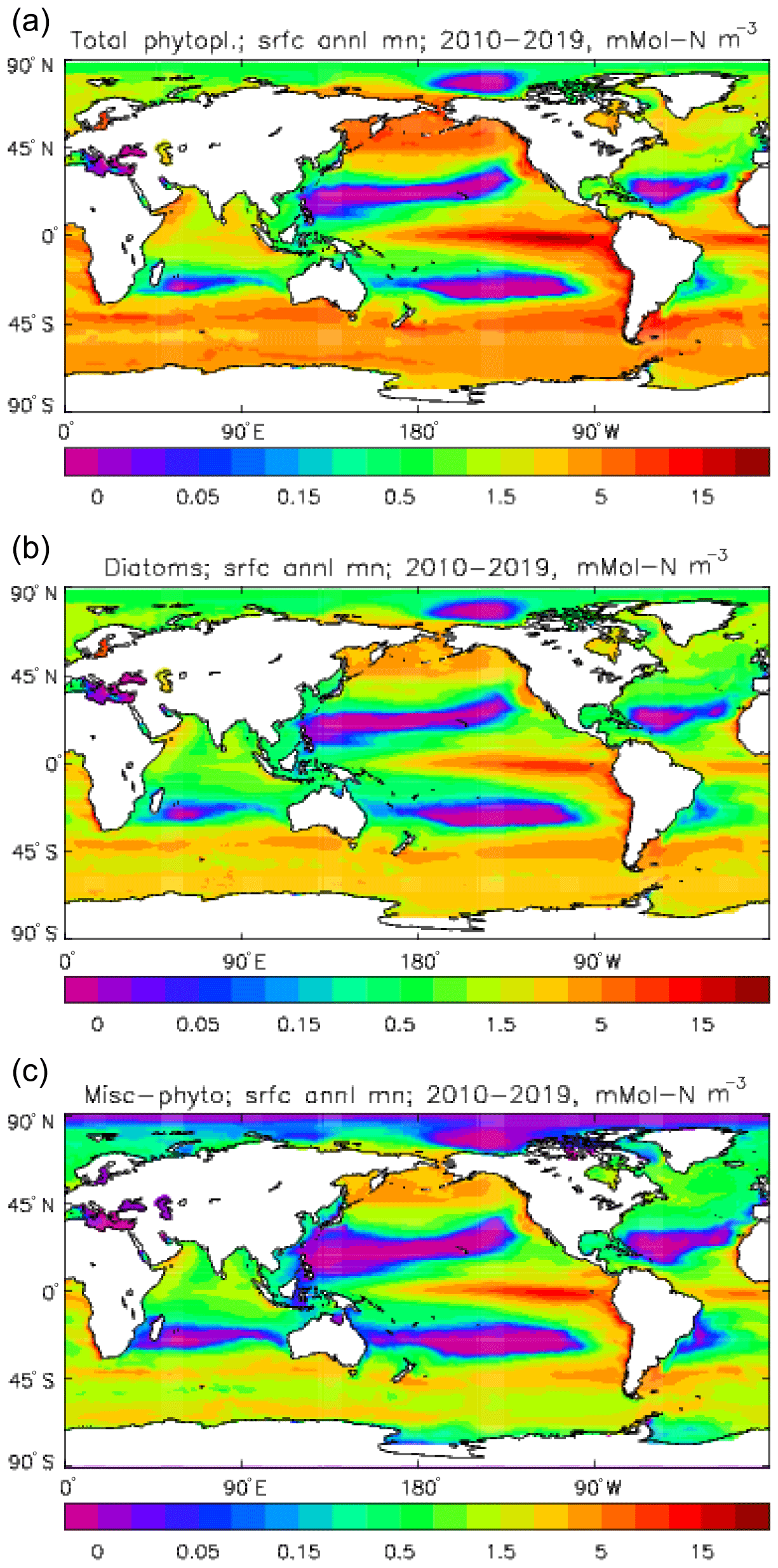
Figure 6Phytoplankton surface biomass (mMol N m−3), averaged over the model years 2010–2019: (a) total phytoplankton; (b) diatoms; (c) misc-phytoplankton.
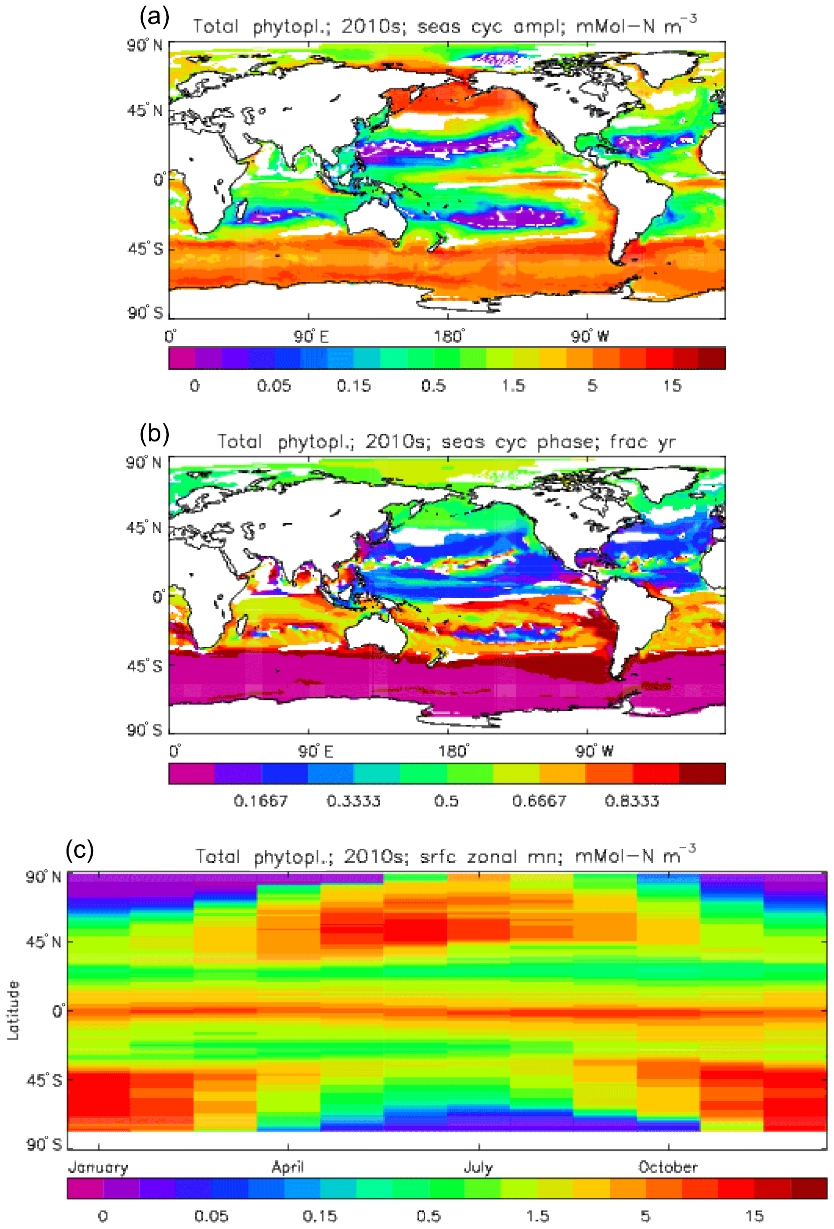
Figure 7Total phytoplankton surface biomass mean seasonal cycle, averaged over the model years 2010 to 2019. (a) Amplitude (mMol N m−3) and (b) phase (fraction of year when peak value occurs) of the seasonal cycle, determined by the best-fitting sine curve (only points for which the residual variance is less than half that of the original cycle are shown). (c) The global zonal mean for each month (mMol N m−3).
3.1 Simulations
The HadGEM2-ES model was used to run a wide range of simulations for CMIP5, the 5th Climate Model Intercomparison Project (Taylor et al., 2012). Jones et al. (2011) give a detailed overview of the HadGEM2-ES simulations. The results presented here relate to a subset of three simulations, all with a prescribed atmospheric CO2 concentration. The first is the pre-industrial control (“piControl” in the CMIP5 terminology), the historical simulation (“historical”; from December 1859 to December 2005) and the RCP8.5 future simulation (“RCP8.5”). The historical simulation branched from the piControl, and RCP8.5 was a continuation of the historical to simulated year 2100.
The model was spun up before the piControl commenced. The ocean has particular issues with spin-up because ideally several cycles of the ocean overturning circulation are needed to bring the tracers into equilibrium with the circulation and the driving climatological fluxes from the atmosphere, and each cycle lasts 500–1000 model years. It was therefore deemed impractical to spin the full coupled model for the required time, and in any case the atmosphere and land-surface models would reach equilibrium much faster.

Figure 8Total primary production, depth integrated and averaged over the model years 2010–2019: (a) decadal mean (g C m−2 d−1); (b) zonal mean for each month, same units; (c) amplitude of model seasonal cycle (best-fitting sine curve), same units; (d) phase of model seasonal cycle (units are fraction of year when peak value occurs). As described in the text, the seasonal cycle has been determined by the best-fitting sine curve, and points are only shown for which the variance of the residual cycle is less than half that of the original cycle.
The World Ocean Atlas (hereafter WOA) provides comprehensive gridded fields for the active tracers, temperature and salinity, and the processes affecting these quantities at the surface are relatively well understood and parameterised, so it was possible to initialise the ocean with fields close to equilibrium. The biogeochemical tracer fields, however, were not so easy to initialise. WOA gridded fields are available for the nutrients nitrate and silicate and for oxygen, but they are based on many fewer data than those for temperature and salinity. Gridded fields are available for dissolved inorganic carbon (DIC) and total alkalinity (TAlk) from GLODAP (Sabine et al., 2005; Key et al., 2004), but these are based on even fewer data and relate to the present day with a substantial storage of anthropogenic carbon rather than the pre-industrial distribution (a correction for anthropogenic storage is available, but the method used for its production introduces many more uncertainties). At the time that the model spin-ups were started the 2009 edition of the WOA database was the most recent, so those fields were used. In addition, while the Diat-HadOCC model was developed to represent the main ocean biogeochemical processes which (along with the physical circulation) determine the horizontal and vertical distributions of these tracers, incomplete knowledge of these processes, particularly quantitatively, and the model's necessary simplicity mean that the simulated fields may be significantly different from those measured in the real ocean (even with an accurate circulation). Therefore, the ocean biogeochemical tracers, even if initialised from the best-available gridded fields, required a significant period of spin-up before the drifts became acceptably small. The main criterion for “acceptably small” was a net pre-industrial air–sea flux of CO2 that was below 0.2 Pg C yr−1 (averaged over a decade, so inter-annual variability was smoothed out).
The tracers were therefore initialised as follows.
-
Temperature and salinity: WOA 2009; Locarnini et al. (2010), Antonov et al. (2010).
-
Nitrate, silicate (i.e. silicic acid) and oxygen: WOA 2009; Garcia et al. (2010a, b).
-
Iron: an initial field was produced from measurements reported in Parekh et al. (2004), on which the iron model used in Diat-HadOCC was based.
-
Misc-phytoplankton, diatoms, zooplankton, and also C, N and Si detritus: a nominal small value (10−6 mMol m−3) was used because these quantities (being mainly confined to the surface levels) would very quickly come into a pseudo-equilibrium with the climatological fluxes and the initial nutrient distributions and then be able to track the decadal and centennial changes to those distributions.
-
DIC and TAlk: these were initialised from (re-gridded) fields from an earlier pre-industrial simulation by the HadCM3C model, wherein the net air–sea CO2 flux had been within the criterion; it was expected that the large-scale ocean circulation would not differ greatly between the models.
The early stages of the spin-up were done incrementally: while parameterisations of the land-surface and dust sub-models were being tested, 40-year simulations were run for each trial sequentially, and around 200 years of spin-up were obtained this way. It was reasoned that the different versions of the land and dust models would not produce significantly different equilibria for the ocean tracers, and the ocean biogeochemical model, which was unchanged, would be a more dominant influence. After this period, another 100 years of simulation was completed with the finalised model, and during this average fields (one for each month of the year) were calculated for the climatological fluxes between the atmosphere and ocean. These average annual cycle fields were then used to force a coarse-resolution ocean-only model (a low-resolution version of the ocean component of HadCM3 – see Gordon et al. (2000) – with Diat-HadOCC embedded) which could be run extremely efficiently. This ran for 2000 simulated years, after which the biogeochemical fields (but NOT temperature or salinity) were re-gridded back to the HadGEM2-ES ocean resolution and put back in that model (at the point immediately following the 100-year coupled spin-up). HadGEM2-ES was subsequently run in coupled mode for a further 50 years, during which it was found that the main criterion of the net air–sea CO2 flux being below 0.2 Pg C yr−1 was comfortably satisfied, and the drifts in the other biogeochemical fields were reduced compared to before the ocean-only phase. However, there were still significant drifts in the silicate and dissolved iron fields: in the pre-industrial control simulation the silicate concentration in the top 100 m increased by around 4.8 and 3.3 mMol Si m−3 during the first and second centuries, respectively, while that in the lowest 2000 m decreased by around 4.0 and 2.2 mMol Si m−3, and the dissolved iron increased at all depths, in the top 100 m by 0.12 mMol Fe m3 per century and below 1000 m by 0.055 mMol Fe m3 per century.
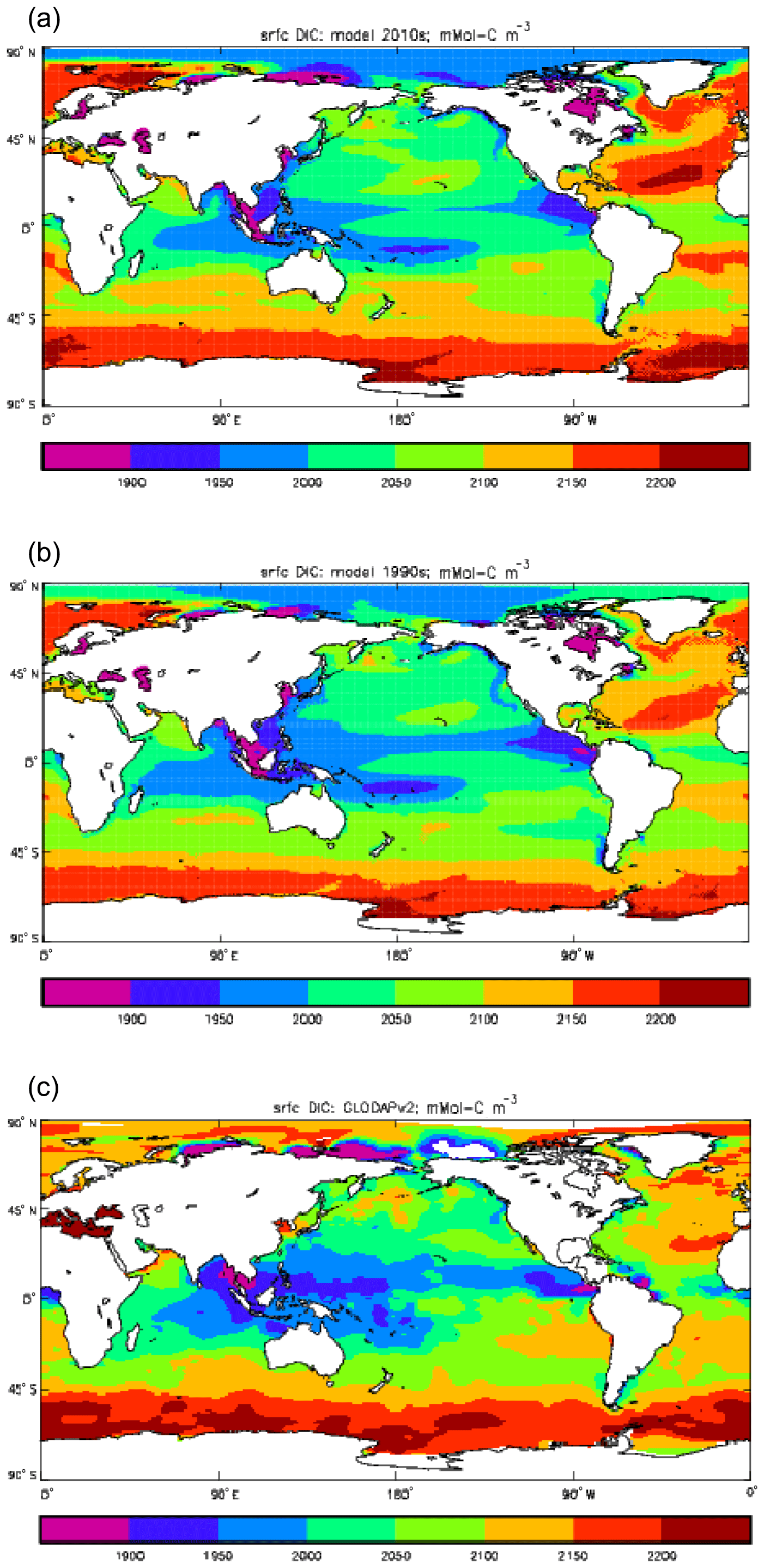
Figure 9Surface concentration of dissolved inorganic carbon (mMol C m−3): (a) model field averaged over model years 2010–2019; (b) model field averaged over model years 1990–1999; (c) the gridded field from the GLODAPv2 database.
The pre-industrial control (piControl) simulation was started from the end of the coupled spin-up, with its date set to 1 December 1859. (Note that HadGEM2-ES, like previous Met Office climate models, uses a 360 d year of 12 months, each of 30 d, and begins its simulations on 1 December, the start of meteorological winter, rather than 1 January.) It ran to the year 2100 and beyond. The atmospheric CO2 concentration was prescribed at a constant value, and the concentration (strictly, the partial pressure) seen by the ocean was also held at the same constant value. The historical simulation began from the same date using the same initial fields. It ran to the end (31 December) of 2005. The atmospheric CO2 concentrations were prescribed according to the CMIP5 dataset (https://pcmdi.llnl.gov/mips/cmip5/forcing.html, last access: 18 October 2019). The future simulation, RCP8.5, began at 1 December 2005 and was initialised using the fields from the historical simulation that were valid for that time. Again, the atmospheric CO2 was prescribed, but this time according to a future scenario (also to be found in the CMIP5 dataset). This was one of four RCPs (Representative Concentration Pathways; see Moss et al., 2010) calculated using an integrated assessment model using projections of future anthropogenic emissions and other changes. RCP8.5 is the scenario with the highest atmospheric CO2 concentrations, and the radiative forcing at the year 2100 due to additional CO2 is 8.5 W m−2. Changes in the Earth system due to climate change will in general show most clearly in this scenario, and so, although HadGEM2-ES ran all four RCP simulations (Jones et al., 2011; which also gives more details of other climatically active gases, for example, in these experiments), it is the results from RCP8.5 that are considered in the following section.
The primary purpose of the Diat-HadOCC model is to represent the marine carbon cycle, along with the factors and feedbacks influencing and controlling it, in the past, in the present and in the future; and therefore initially the results described here relate to those quantities most directly connected with that cycle. However, it is also important to know that where the model results closely agree with observations they do so for the right reasons rather than by coincidence, so certain other quantities are also presented.
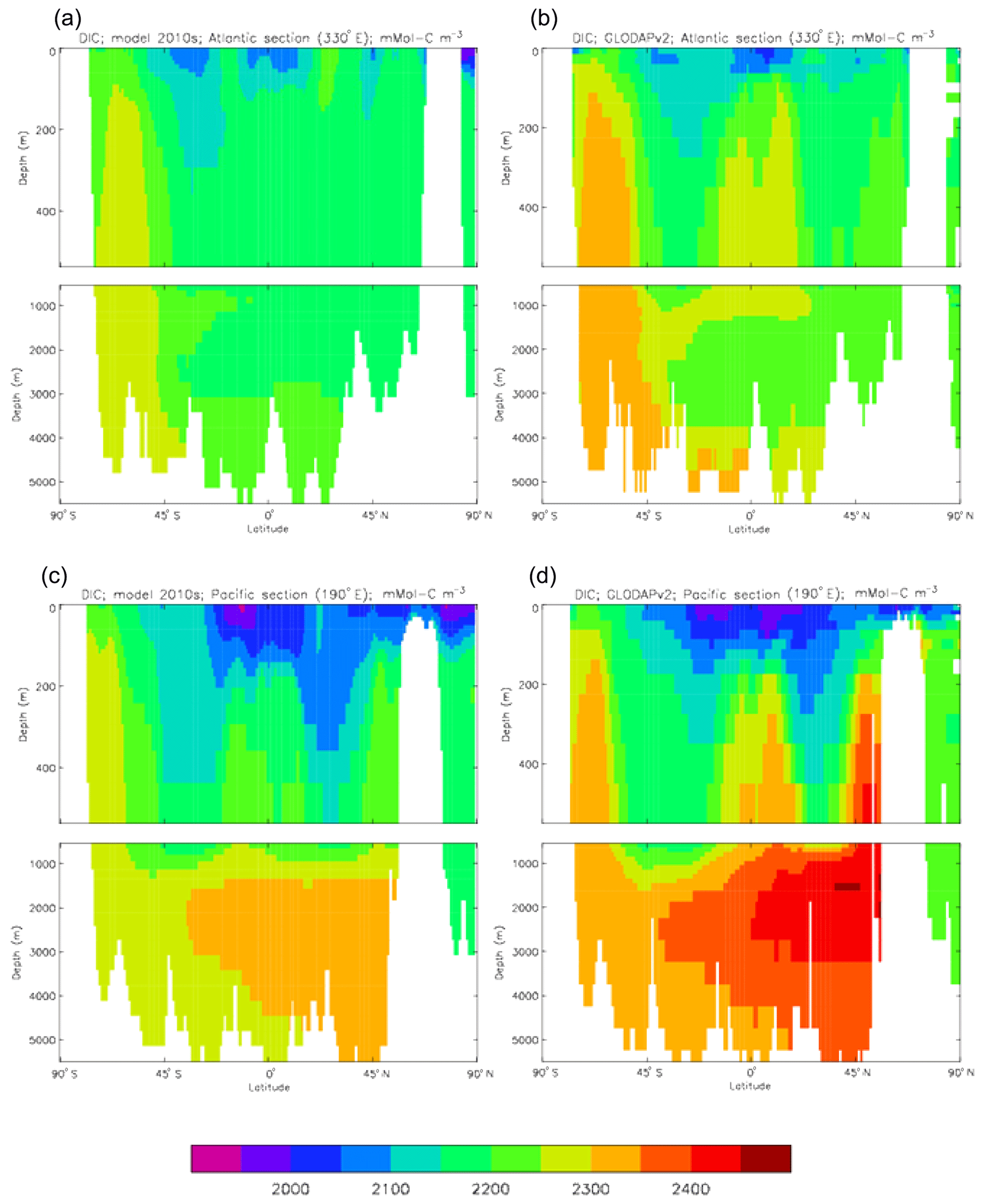
Figure 10Meridional sections of DIC: panels (a) and (b) show sections in the Atlantic Ocean along 330∘; (c, d) Pacific Ocean sections along 190∘. Panels (a) and (c) show model concentrations averaged over 2010–2019, and panels (b) and (d) show concentrations from the GLODAPv2 gridded product.
4.1 Results for the present day (2010s)
4.1.1 Total chlorophyll
Figure 2a shows the annual mean surface total chlorophyll predicted by the model for the (simulated) decade 2010–2019, and that derived from satellite retrievals is in Fig. 2b. The satellite-derived data are from the GlobColour surface chlorophyll product (Fanton d'Andon et al., 2008; Maritorena et al., 2010) for the years 1998–2007, with further processing as described in Ford et al. (2012) to produce a monthly climatology, which has then been averaged to give the annual mean. Two things are immediately apparent: the geographical distributions are similar, but the actual values in the model are noticeably more extreme; they are higher where the data are high (Southern Ocean, subpolar gyres in the North Pacific and North Atlantic, eastern equatorial Pacific) and lower where the data are low (mainly the subtropical gyres). In fact, in the centres of the subtropical gyres the model chlorophyll is very slightly negative. Comparing the area means of the respective annual mean fields, the model has an average of 0.812 mg Chl m−3, while the average of the data is 0.213 mg Chl m−3. However, the seasonal cycle is also important, and Fig. 3a shows the seasonal cycle of the zonally meaned model chlorophyll; Fig. 3b shows the same but scaled by the factor 0.213∕0.812 (so that the global annual mean is the same as that of the data), and Fig. 3c shows the seasonal cycle of the zonally meaned data. It can be seen by comparing Fig. 3b and c that the excess chlorophyll is accentuated by a greater-than-average factor when the observed chlorophyll is high. It is possible to find the best-fitting sine curve through the monthly mean values at any points (assuming they form a repeating cycle); points are only shown for which the variance of the residual cycle (after the best-fitting curve has been subtracted off) is less than half that of the original cycle (meaning that a sine curve is a good 1st-order description of the seasonal cycle). Figure 4a and c show the amplitude and Fig. 4b and d show the phase of the seasonal cycle so derived of the model chlorophyll (panels a–b, amplitude adjusted by factor 0.213∕0.812 so that patterns can be better compared) and the satellite-derived data (panels c–d). In the model, the seasonal cycle is larger (even when adjusted) in much of the Southern Ocean and in the equatorial Pacific and slightly lower in the subpolar North Atlantic. In terms of the phase and high latitudes, there is good agreement between the model and the data, though the model misses the late summer peak that dominates the subpolar North Pacific. In the tropics and subtropics there is less agreement; in particular across all basins, the model shows peak chlorophyll around September–October in the Southern Hemisphere between 10 and 35∘, but the data show the peak occurring 2 to 3 months earlier. Figure 5 compares the model total chlorophyll to the GlobColour product in a Taylor diagram. The mean concentration and the midpoint, amplitude and phase of the sine curve that best fits the seasonal cycle are shown (only points that satisfy the variance condition are considered for the seasonal cycle). Figure 5a shows the comparisons for the actual model results, while Fig. 5b shows those for the model results scaled by the 0.213∕0.812 factor. It can be seen that there is an excellent fit in terms of the standard deviation for the seasonal cycle phase but that correlation is poor, and for the concentrations and cycle amplitude the (unscaled) model greatly overestimates the values (and again the correlation is poor). The scaled comparison is of course better for the standard deviation but shows that the seasonal cycle in the model is generally of lower amplitude compared to the mean than is found in the data. The satellite-derived chlorophyll products usually accurately show very high concentrations in shelf seas and close to the coasts, but models often struggle to show those features: the coarse physical resolution means that in many locations there is no coastal shelf (ocean water columns adjacent to land can be as deep as the rest of the basin) and most models (including HadGEM2-ES) do not represent the tidal mixing processes that in the real ocean are vital to supply nutrients that have been regenerated in the shallow sediments to the surface where they can drive high growth rates. Therefore, the Taylor diagram also shows a comparison (open symbols) that excludes two grid boxes around the coasts so that it is only between open-ocean points. The result is that the model overestimates the concentrations even more, though the correlation is slightly improved.

Figure 11Surface DIC model seasonal cycle, averaged over model years 2010–2019: (a) amplitude of the cycle (mMol C m−3); (b) phase of the cycle (fraction of year). Only points for which the residual variance is less than half the original are shown.
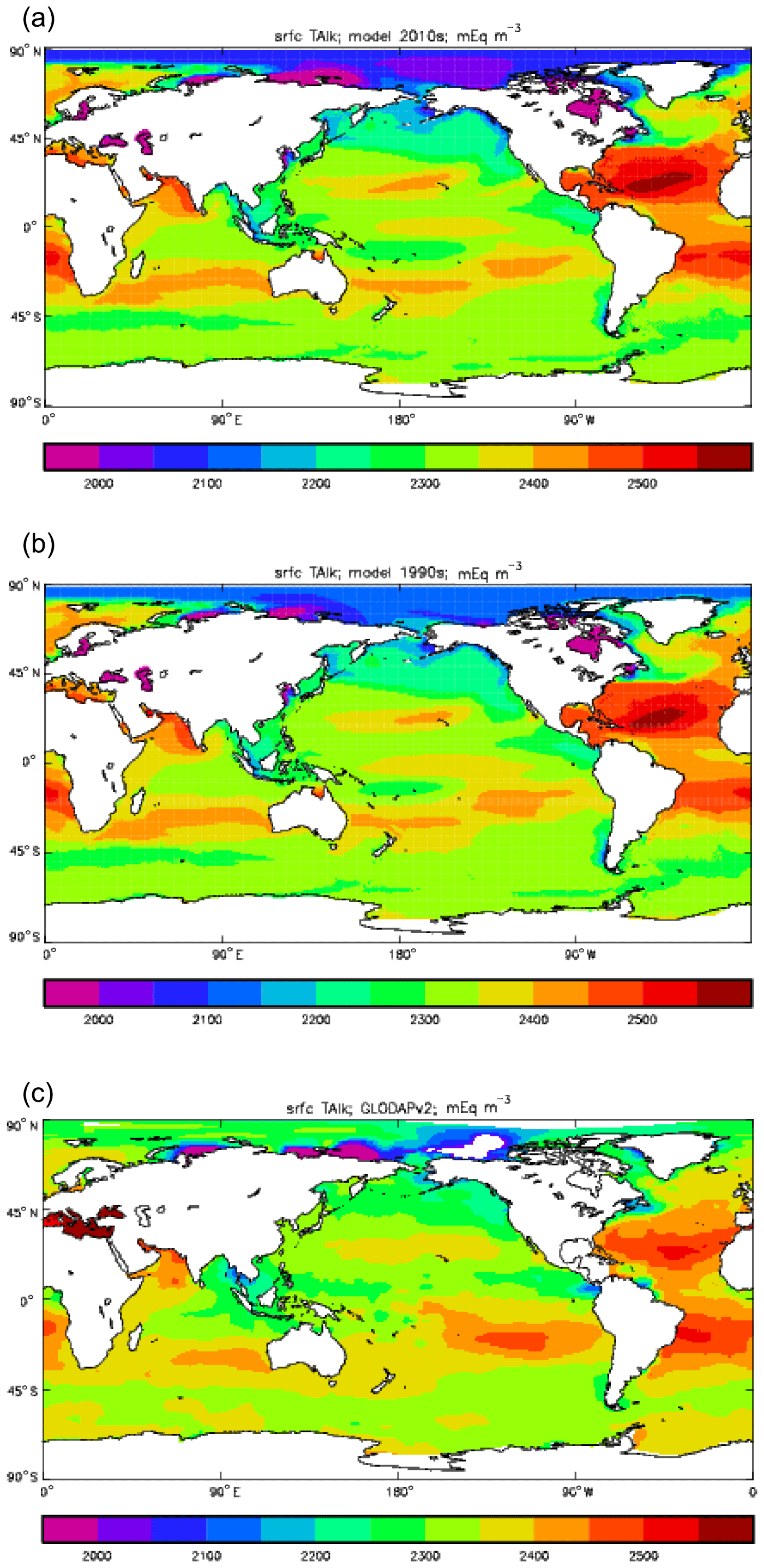
Figure 12Surface concentration of total alkalinity (mEq m−3): (a) model field averaged over model years 2010–2019; (b) model field averaged over model years 1990–1999; (c) the gridded field from the GLODAPv2 database.
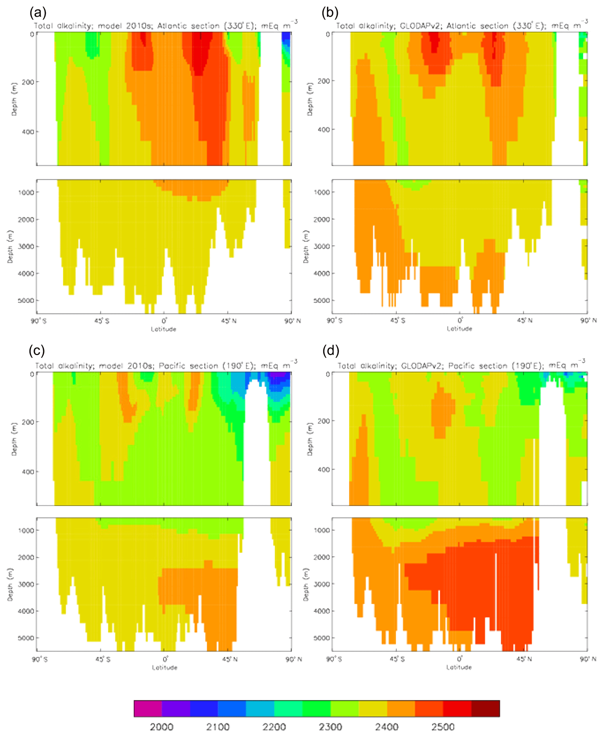
Figure 13Meridional sections of total alkalinity: panels (a) and (b) show sections in the Atlantic Ocean along 330∘; (c, d) Pacific Ocean sections along 190∘. Panels (a) and (c) show model concentrations averaged over 2010–2019; panels (b) and (d) show concentrations from the GLODAPv2 gridded product.
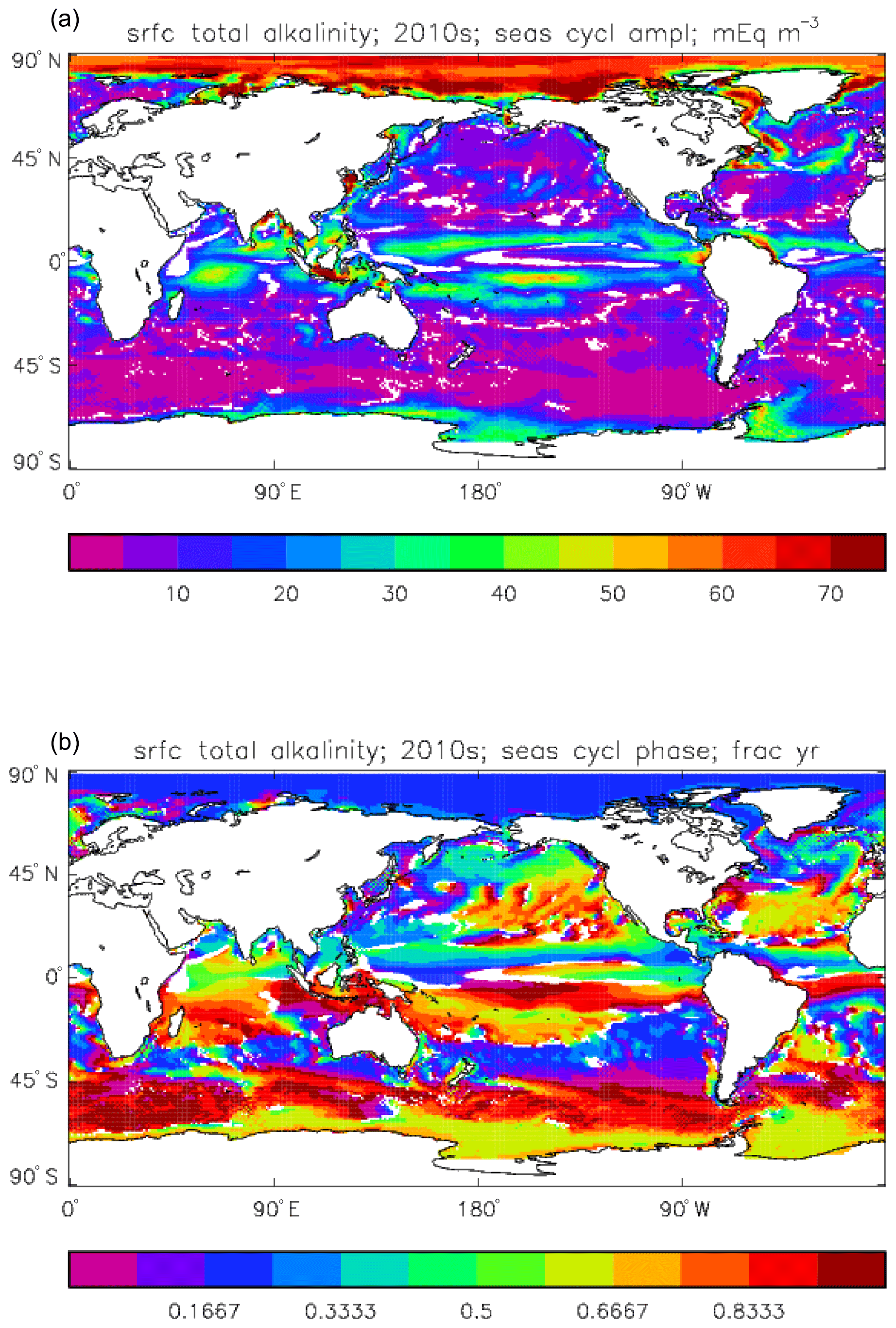
Figure 14Surface total alkalinity model seasonal cycle, averaged over model years 2010–2019: (a) amplitude of cycle (mEq m−3); (b) phase of cycle (fraction of year). Only points for which the residual variance is less than half the original are shown.
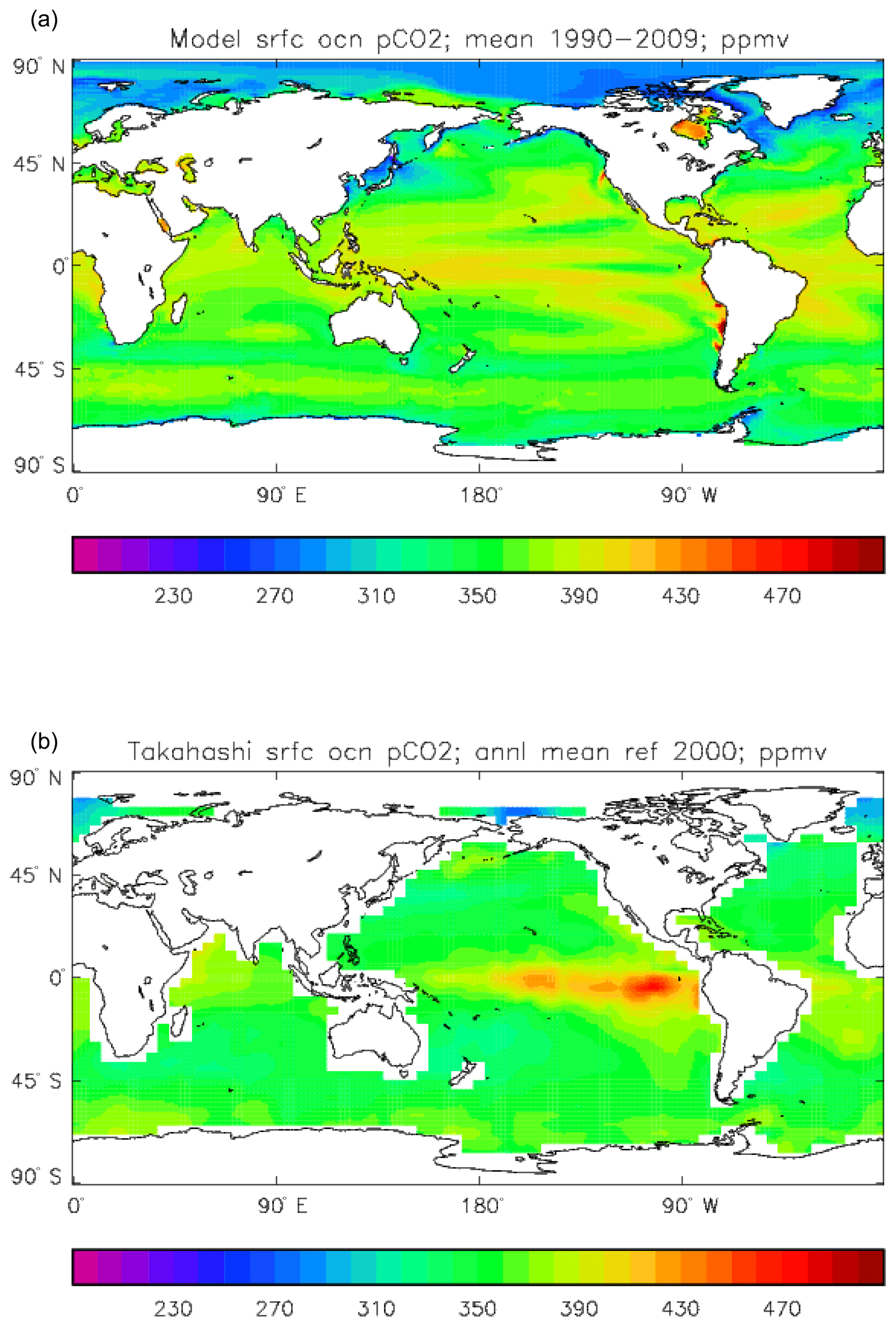
Figure 15Surface ocean pCO2 (ppmv): (a) model field averaged over the model years 1990–2009; (b) Takahashi gridded field from data; annual mean referenced to the year 2000.
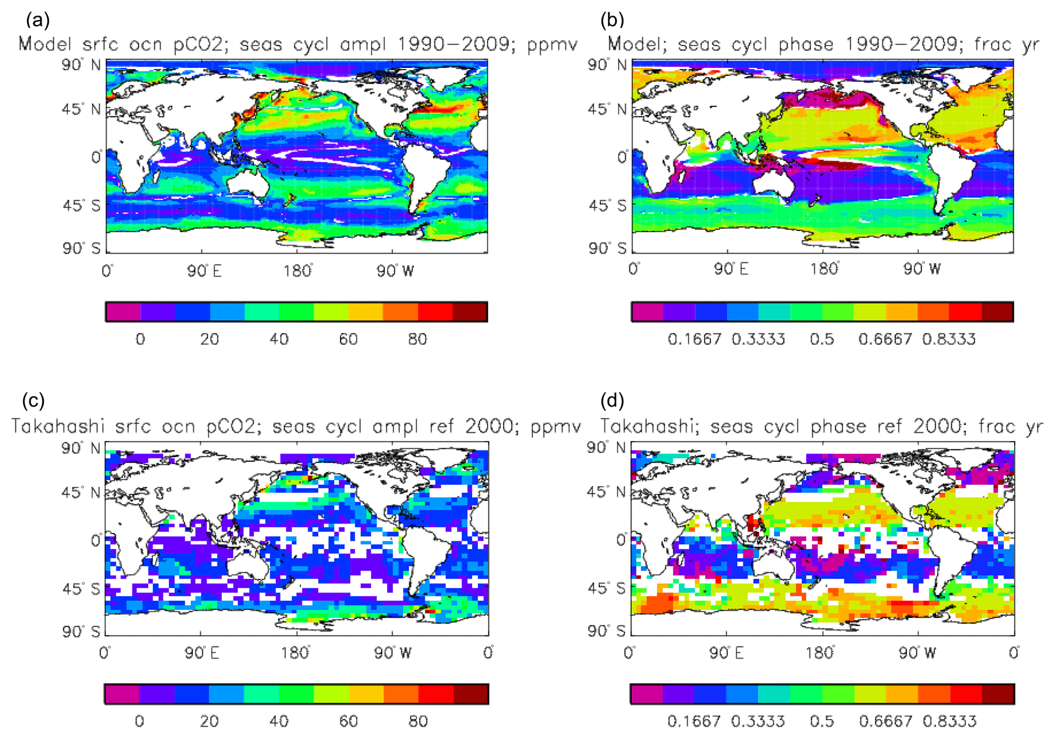
Figure 16Surface ocean pCO2, seasonal cycle: (a, b) model averaged over model years 1990–2009; (c, d) Takahashi gridded data, referenced to the year 2000; (a, c) amplitude of the cycle (ppmv); (b, d) phase of the cycle (in fraction of year). Only points for which the residual variance is less than half the original are shown.
4.1.2 Diatoms and misc-phytoplankton
Figure 6 shows the total surface biomass of phytoplankton (mMol N m−3) and also, separately, that of the two phytoplankton types, diatoms and misc-phyto: the mean for the model years 2010–2019. The geographical patterns are naturally very similar to that of the model's total surface chlorophyll, since the CMIP5 simulations used a fixed carbon:chlorophyll ratio for each of the phytoplankton (and the same value, 40.0 mg C per milligram of chlorophyll, for each type). The geographical patterns for each type are also very similar to each other, with the diatoms having a slightly greater value than the misc-phyto (global averages 1.486 and 1.223 mMol C m−3, respectively, so diatoms make up 55 % of the total surface biomass). The diatoms are slightly more dominant than the global average in the North Atlantic Ocean and in the Southern Ocean, both areas where surface silicic acid (needed by diatoms for shell formation) is plentiful. An issue with these results is that the distributions of the two phytoplankton types are more similar than they should be. This is due to two factors: the parameter values used (for growth rate) are similar, and the concentrations of dissolved silicate and dissolved iron, which should produce contrasting responses in the two types, are less limiting in the model than they are in the real ocean and so fail to distinguish them. In terms of the parameter values, the growth rate of diatoms was 1.85 d−1 iron replete and 1.11 d−1 iron deplete, while that of misc-phytoplankton was 1.50 d−1, and diatoms had a sinking rate of 1.0 m d−1, while misc-phytoplankton did not sink, but the majority of other parameters were identical and there was no difference between the iron-replete and iron-deplete values when those could vary (except the diatom growth rate, as described above). These parameter choices were made after a limited sensitivity analysis that was constrained by the time and computing resources available, and it was reasoned that only if that analysis showed a significant reason for choosing different values for corresponding diatom and misc-phytoplankton parameters should they not be identical. The surface silicate concentration was, during the historical and future RCP simulations, much too high because the dissolution (remineralisation) rate was too high, so diatom growth was not restricted by silicate limitation in areas and in parts of the seasonal cycle when it should have been. In particular, the diatoms do relatively well in the oligotrophic gyres compared to misc-phytoplankton because they have a nitrate half-saturation constant that is not very different (in absolute terms) from that of the misc-phytoplankton and the erroneously high silicate concentration does not limit their growth; in the real ocean they would be strongly silicate limited in these areas and their large cell size would mean they were at a competitive disadvantage compared to other phytoplankton. Similarly, the surface iron concentration was higher than observed in many parts of the ocean and so did not limit the production at times and places when it should have. These factors mean that the ability of the model to represent two different phytoplankton has not been explored as well as was intended. Figure 7 shows the amplitude and the phase of the seasonal cycle of the total surface biomass and also a Hovmöller diagram of the zonal mean seasonal cycle. As in the case of the total chlorophyll, the amplitude and phase have been obtained by fitting a sine curve to the monthly mean values at each point. The amplitude of the cycle is very similar to the mean biomass, except in the equatorial latitudes (especially in the equatorial Pacific) where the amplitude is significantly less; this implies that in those latitudes there is significant biomass all year round, whereas in the high latitudes where the cycle amplitude and the mean are similar the biomass drops to near zero for at least some of the year. The phase of the seasonal cycle of surface biomass (time of year of the maximum) is very similar to that of total surface chlorophyll, as is to be expected. The Hovmöller diagram clearly shows the poleward progression of the high-latitude blooms.
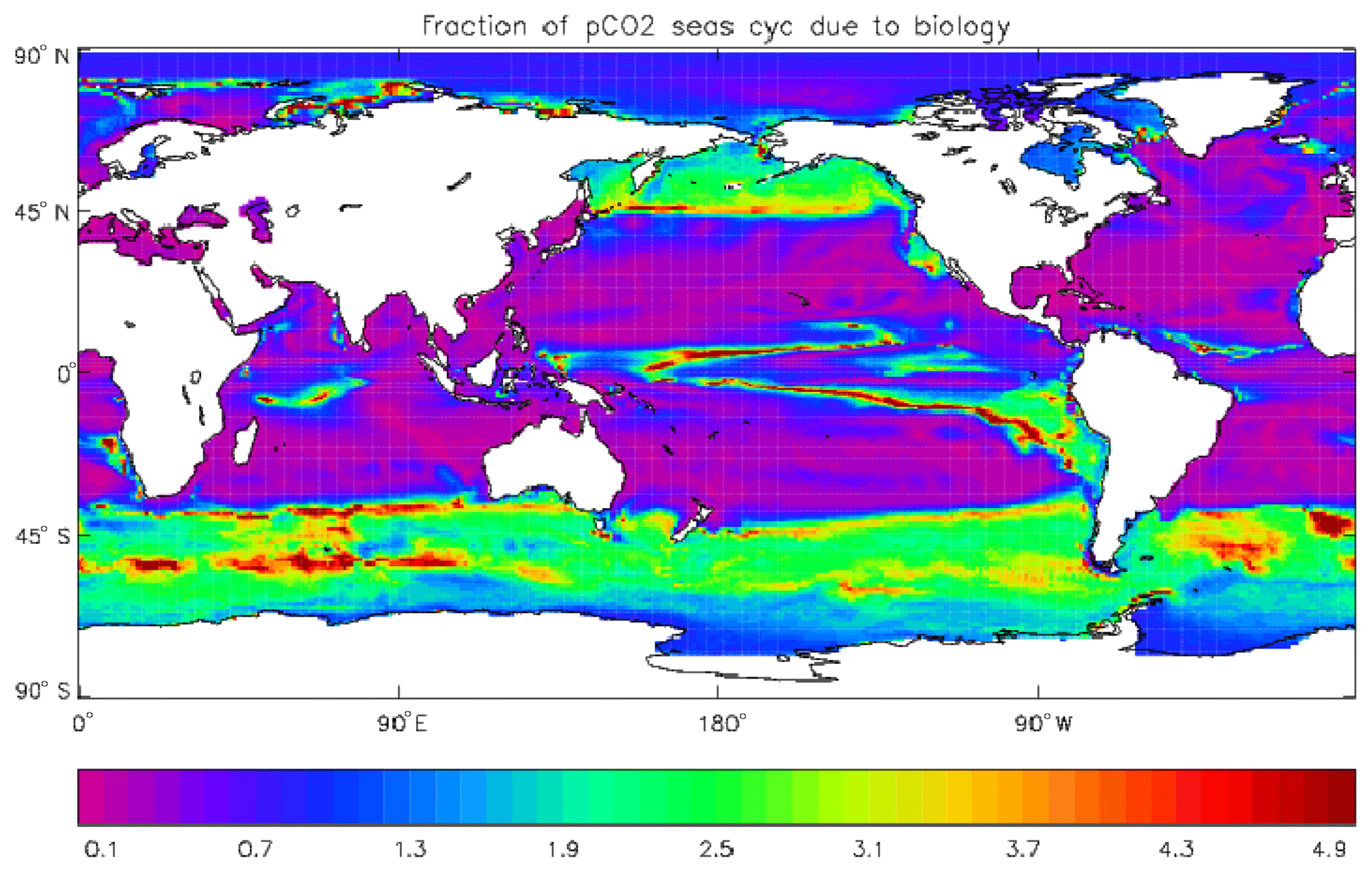
Figure 17Fraction of the seasonal cycle of pCO2 that is not driven by the temperature (and salinity) seasonal variation. The details of the calculation are given in the text. Where the ratio is less than 0.5, the temperature variation dominates, and where the ratio is greater than 0.5 the biological uptake and respiration (and the air–sea uptake) dominate. Ratios greater than 1.0 indicate that the biologically driven and temperature-driven cycles are opposed.
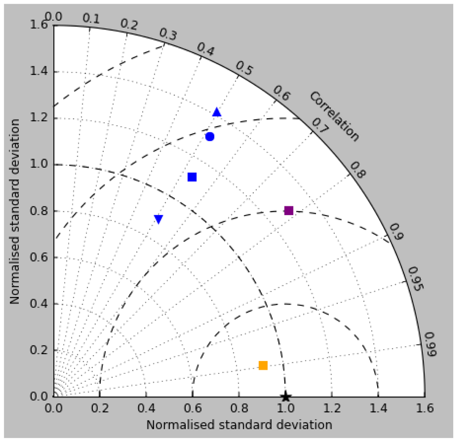
Figure 18Taylor diagram for surface DIC (orange), surface total alkalinity (purple) and surface pCO2 (blue). Model DIC and total alkalinity from the RCP8.5 simulation (meaned over the years 2010 to 2019) are compared to the gridded fields from GLODAPv2, while model pCO2 (meaned over 1990 to 2009) is compared to the Takahashi gridded data. Filled squares refer to the raw surface fields, and filled circles, upward-pointing triangles and downward triangles respectively refer to the midpoint, amplitude and phase of the sine curve that best fits the seasonal cycle (in points for which the variance of the residual is less than half that of the original cycle).
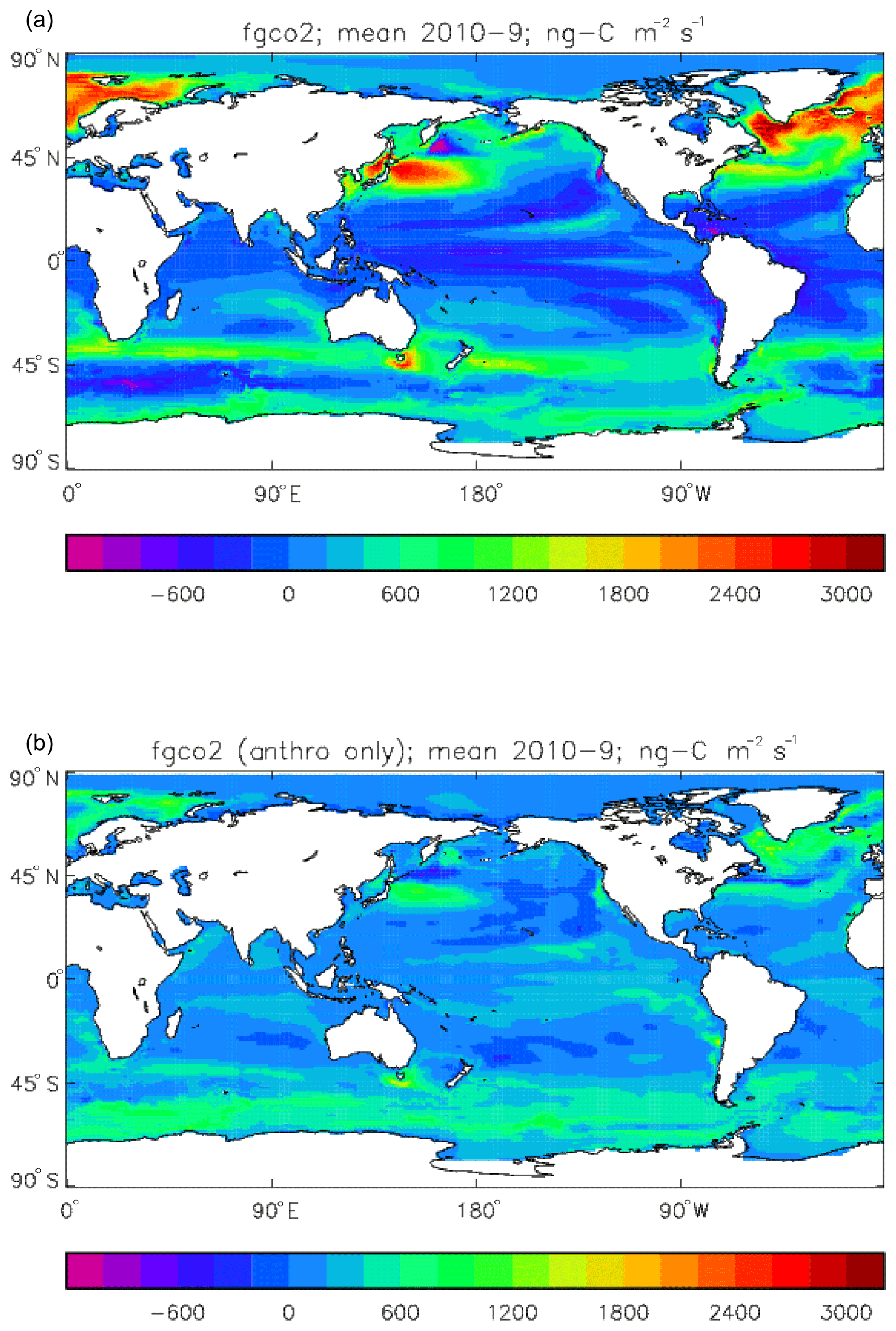
Figure 19Total air-to-sea flux of CO2 (ng C m−2 s−1; positive values into the ocean), mean over model years 2010–2019: (a) total flux (natural cycle and anthropogenic perturbation); (b) anthropogenic perturbation.
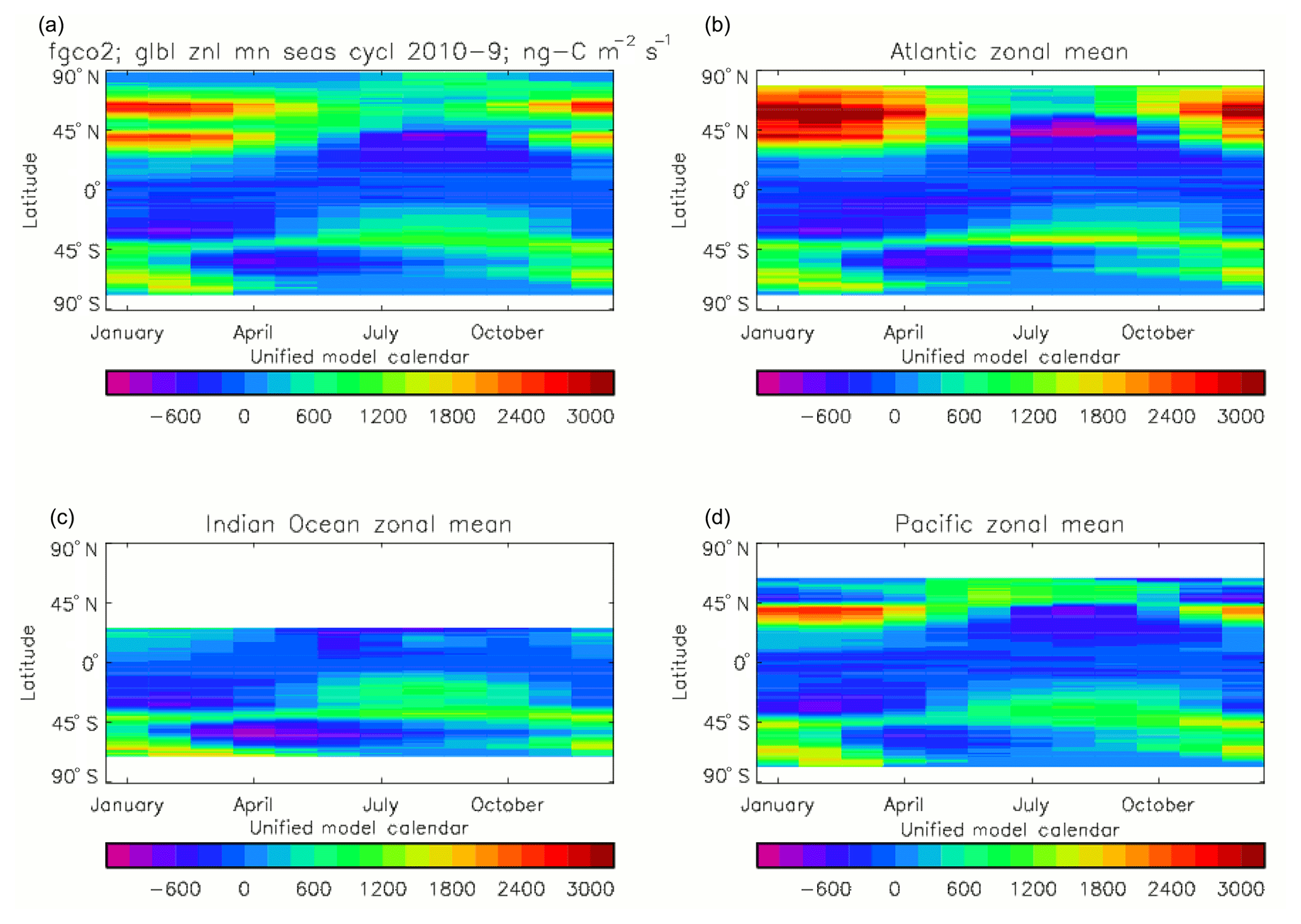
Figure 20Total air-to-sea flux of CO2 (ng C m−2 s−1), seasonal cycle averaged for each month over the model years 2010–2019, zonally meaned: (a) global zonal mean; (b) zonal mean of the Atlantic Ocean basin; (c) zonal mean of the Indian Ocean basin; (d) zonal mean of the Pacific Ocean basin.
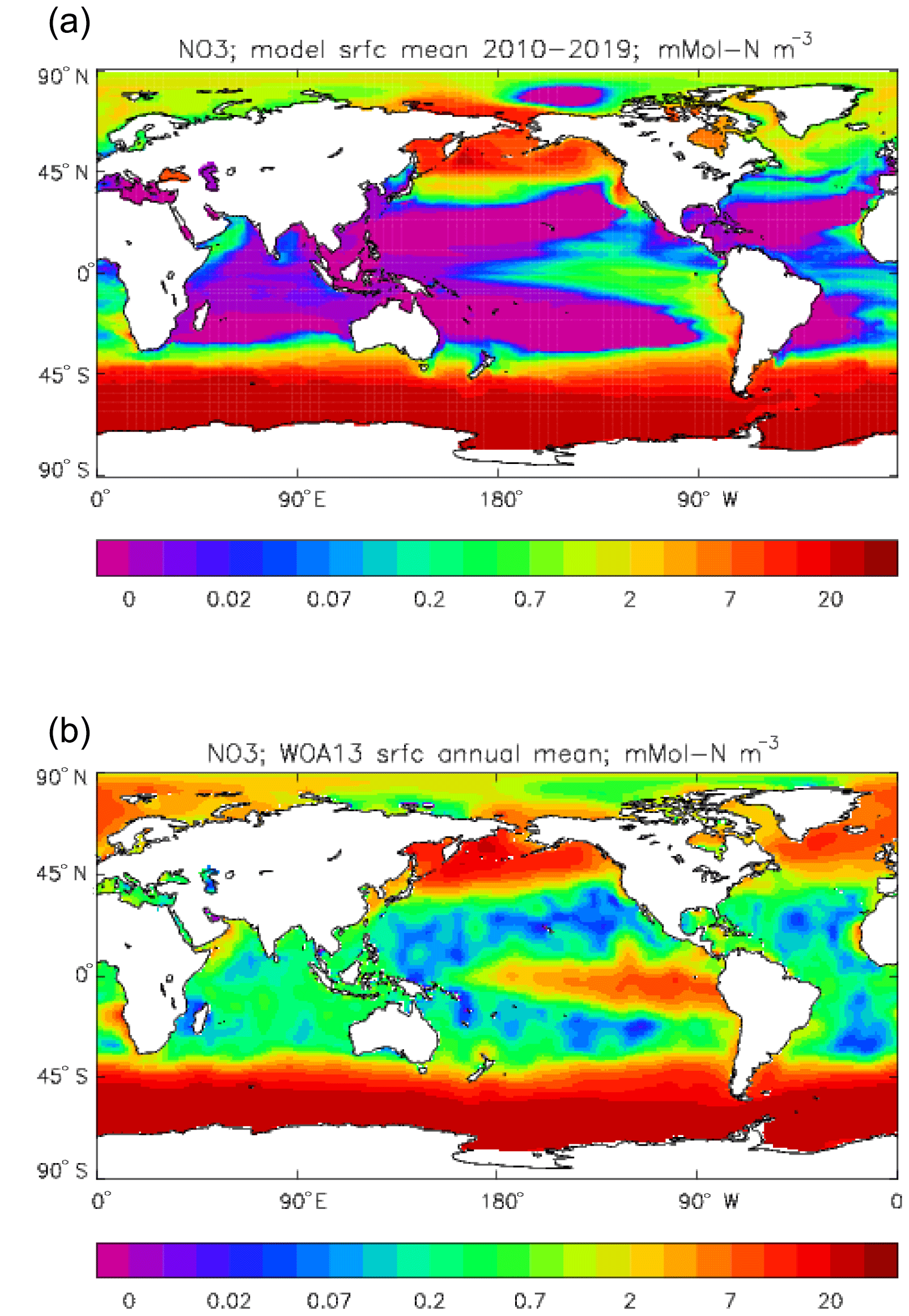
Figure 22Surface dissolved nitrate (mMol N m−3): (a) model field averaged over model years 2010–2019; (b) the gridded field from the 2013 World Ocean Atlas.
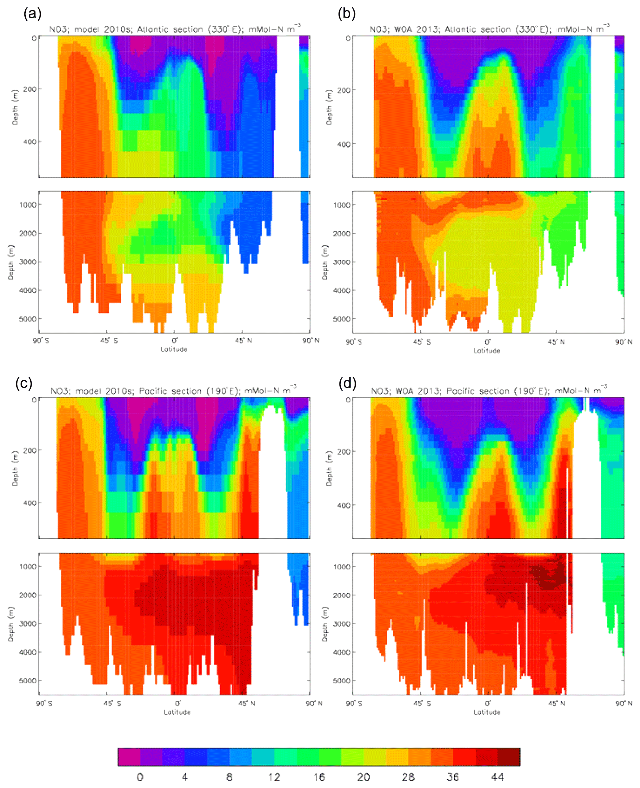
Figure 23Meridional sections of dissolved nitrate (mMol N m−3): panels (a) and (b) show sections in the Atlantic Ocean along 330∘; (c, d) Pacific Ocean sections along 190∘. Panels (a) and (c) show model concentrations averaged over 2010–2019; panels (b) and (d) show concentrations from the 2013 World Ocean Atlas gridded field.
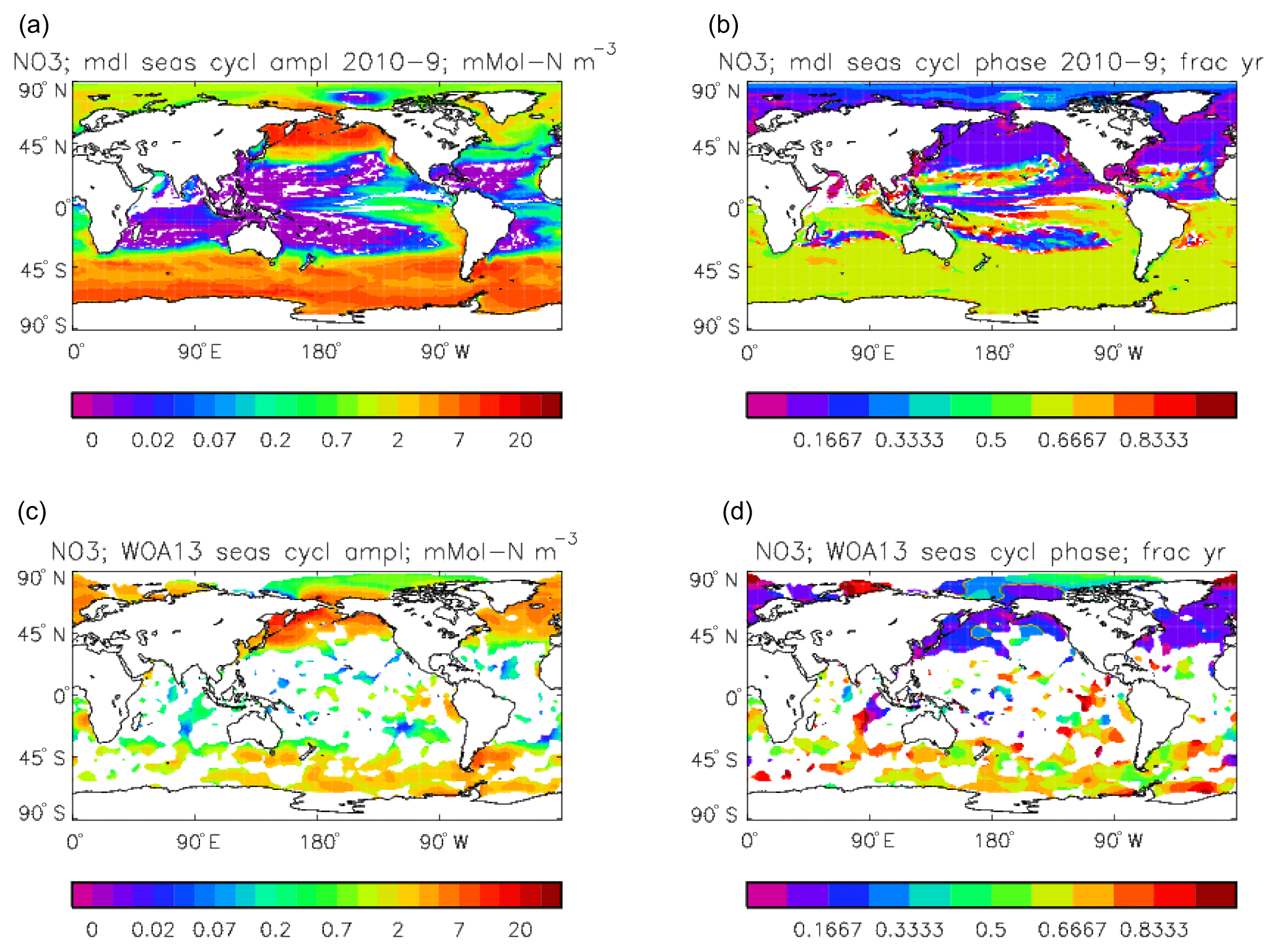
Figure 24Surface dissolved nitrate seasonal cycle: (a, b) model cycle, averaged over model years 2010–2019; (c, d) the cycle from the monthly gridded fields from the 2013 World Ocean Atlas; (a, c) the amplitude of the cycle (mMol N m−3); (b, d) the phase of the cycle (fraction of year). Only points for which the residual variance is less than half the original are shown.
4.1.3 Primary production
The vertically integrated global total primary production during the years 2010–2019 in the model is 35.175 Pg C yr−1; of this 19.791 Pg C yr−1 (56.3 %) is due to the diatoms and 15.384 PgC yr−1 is due to the misc-phyto. The total is slightly below the generally quoted range of global primary production, 40–60 Pg C yr−1 (e.g. Carr et al., 2006). However, that total includes the high-production areas along the coasts and in shelf seas, which the coarse physical resolution and the structure of the model do not allow to be realistically represented: there are no sediments, no tidal mixing, and no riverine supply of nutrients or run-off from land, and the circulation over the shelf (where that exists) is not accurate. Figure 8 shows the total primary production (gC m−3 d−1). The geographical pattern (of the decadal mean, panel a) is very similar to that of the total phytoplankton biomass in Fig. 6, as expected. The Hovmöller diagram of the seasonal cycle of the zonal mean (panel b) is also very similar to that in Fig. 7. The geographical patterns of the amplitude (panel c) and the phase (panel d) of the seasonal cycle (determined, as before, by the best-fitting sine curve, with only points satisfying the variance condition shown) have many similarities with the corresponding plots for total biomass, though relative to its mean the amplitude of the production cycle in the subpolar North Atlantic is greater than that of the biomass. The poleward progression of the peak of the production can clearly be seen in the plot of the phase.
4.1.4 Export flux
The export flux of particulate organic matter at 100 m in the model during the 2010s decade is 5.58±0.11 Pg C yr−1, of which 4.95 Pg C yr−1 is due to sinking detritus and 0.63 Pg C yr−1 due to sinking living diatoms. This gives an export ratio of 0.16. The flux figure is at the lower end of the range found in other studies: Bopp et al. (2013) find a range of 4.9 to 8.1 Pg C yr−1 from a range of CMIP5 models (including HadGEM2-ES), while Siegel et al. (2014) find a slightly wider range of 4.0 to 9.1 Pg C yr−1 using satellite-driven biogeochemical models (and this latter study considers export out of the euphotic zone rather than through a 100 m depth horizon). Figure 2 of the review of Boyd et al. (2019) indicates a range of 4 to 9 Pg C yr−1 for the sinking flux process as represented in this model, but it indicates between 1 and 7 Pg C yr−1 of total additional export due to other “particle injection processes”, of which only the weakest two are represented explicitly in HadGEM2-ES (and not included in the export flux reported here). The calcium carbonate export is 0.26 Pg C yr−1, giving an effective rain ratio of 0.053. This is equal to the formation of calcium carbonate, since in the model none is redissolved above the lysocline.
4.1.5 DIC
Figure 9 compares the model's surface DIC (means over the years 2010–2019 in panel a and 1990–1999 in panel b) with that from the GLODAPv2 gridded field (panel c). The data from the second release of the GLODAP project (downloaded from https://www.nodc.noaa.gov/ocads/oceans/GLODAPv2/, last access: 18 October 2019) have been re-gridded to the HadGEM2-ES ocean grid and converted from moles of carbon per kilogramme of seawater (mol C kg−1) to millimoles of carbon per cubic metre (mMol C m−3) using a mean surface water density of 1025 kg m−3. The global mean surface values are 2068 mMol C m−3 for the model in the years 2010–2019 (and 2054 mMol C m−3 averaged over the years 1990–1999), while the data (referenced to the year 2000) have a global average of 2066 mMol C m−3. Both these quantities, of course, include anthropogenic CO2 present in the surface waters. The geographical pattern can be seen to be very similar, with the only area showing significant disagreement being the Atlantic Ocean basin, in particular the Northern Hemisphere subtropical and subpolar gyres therein, where the surface concentration in the model is significantly higher. There has been a substantial increase in the model's surface concentration in that basin between the 1990s and the 2010s, and the agreement between the model and data is noticeably better for the earlier date (which is closer to the data reference date).
Figure 10 compares meridional sections of the model's DIC concentration to the gridded GLODAPv2 field in the Atlantic Ocean (panels a, b; along 330∘) and in the Pacific Ocean (panels c, d; along 190∘). In the Atlantic section the model underestimates the concentration in the Southern Ocean below about 150 m of depth (the surface values there are comparable, so the gradient in the upper 200 m is too weak in the model), in the Antarctic Intermediate Water (AAIW) and in the bottom water (below 4000 m). These last two errors will be related to the underestimation of the deep Southern Ocean concentration (since that is a source for the AAIW and the bottom water), but the physical model also under-produces AAIW and does not transport what it does produce far enough north. Outside those regions, however, the model's representation is good. In the Pacific section the model underestimates the concentration throughout the section below 1000 m, up to depths as shallow as 200 m in the Southern Ocean, under the Equator and around 45∘ N (all sites where there is significant upward vertical transport). In particular, the model substantially underestimates the meridional gradient between 1000 and 3000 m of depth: the increase from south to north is up to 150 mMol C m−3 in the gridded data but only around 50 mMol C m−3 in the model. This reduced gradient is also seen in total alkalinity and (to a reduced extent) in dissolved nitrate, so the physical deep circulation is likely to be at least a partial cause.
Figure 11 shows the amplitude and the phase (time of year of the maximum) of the seasonal cycle of surface DIC. This is determined by a number of factors: vertical mixing, vertical transport, air–sea CO2 flux, and biological uptake and release. All of these factors vary seasonally and their relative contributions are different from place to place, so the phase of the cycle (and how well a sine curve represents it) varies more with location than many other cycles. In the subpolar North Atlantic, for example, relatively high DIC water is mixed (by convective and wind-induced mixing) from depth to the surface during the winter, and the low surface temperature keeps the ocean pCO2 lower than the atmosphere, so there is ingassing of CO2. As the season passes to spring the increased solar irradiance warms the surface water, vertical mixing is suppressed, and there is net uptake of DIC by the phytoplankton for growth. Those factors tend to cause a reduction in surface DIC concentration and so reduce the pCO2, but at the same time the increased temperature will increase it (for a given DIC concentration); which is the dominant effect, and so whether the air–sea CO2 flux moves towards greater ingassing or greater outgassing, depends on the local conditions. The phase varies by up to 6 months across the North Atlantic at a latitude of 50∘, while at a similar latitude across the Pacific the phase is almost constant.
4.1.6 Total alkalinity
Figure 12 compares the model's surface total alkalinity (means over the years 2010–2019 in panel a and 1990–1999 in panel b) with that from the GLODAPv2 gridded field (panel c; Lauvset et al., 2016, and Key et al., 2015). As with the corresponding DIC plot (Fig. 9) the data from the GLODAPv2 project have been re-gridded to the model grid and converted using a mean water density of 1025 kg m−3 to the model units, in this case millimolar equivalents per cubic metre (mEq m−3). The model's global surface mean values are 2343 mEq m−3 in the 1990s and 2340 mEq m−3 in the 2010s, while the global surface average of the gridded data is 2352 mEq m−3; the approximately 10 mEq m−3 deficit in the model compared to the data is consistent with the 12 mMol C m−3 deficit in 1990s surface DIC compared to the DIC surface data (referenced to the year 2000). The model's total alkalinity is high in the subtropical gyres, especially in the Atlantic Ocean, and this pattern is also seen in the GLODAPv2 gridded field. The correlation between the 2010s model surface field and the (re-gridded) data is 0.78, and the ratio of the standard deviations is 1.29, as shown in Fig. 18; these figures are consistent with Fig. 12, wherein the highest concentrations in the Atlantic are higher than the corresponding highs in the data. Compared to DIC, the correlation is lower, and the ratio is higher.
The biological processes that affect the model's total alkalinity are shown in Eq. (4) to be solid calcium carbonate formation and dissolution and processes linked to the uptake of dissolved nitrate (inorganic nitrogen). At the ocean surface these processes are in opposition (net uptake of DIN and formation of solid carbonate) but, given the low value (0.0195 mMol CaCO3 (mMol C)−1, corresponding to a rain ratio of about 0.053) chosen for the molar ratio of carbonate formation to organic production for misc-phytoplankton and the proportion of primary production due to that phytoplankton type, the effect of the DIN uptake (organic production) dominates. In mid-depths of the model, for example between 500 and 1500 m, there is no carbonate formation or dissolution and no organic growth, but there is significant remineralisation of sinking detritus, which releases nitrate into the water and, since the model links that with an uptake of hydroxyl ions, reduces the total alkalinity in that depth range. Conversely, in depths below the model lysocline (fixed at 2113 m) there is no organic growth or carbonate formation, and what little remineralisation does occur is greatly outweighed by carbonate dissolution, which increases the local alkalinity in the bottom waters. Therefore the general biological effect on total alkalinity should be an increase in deep water and at the surface but a decrease in mid-water. Figure 13 compares meridional sections of the model's total alkalinity to the gridded GLODAPv2 field in the Atlantic Ocean (panels a, b; along 330∘) and in the Pacific Ocean (panels c, d; along 190∘). In the Atlantic it is confirmed that the model overestimates the concentration in the top 1000 m between 40∘ S and 40∘ N, especially north of the Equator, and underestimates the concentration in the Antarctic Bottom Water (AABW). In the Pacific there is an underestimate in the upper water column under the Equator in the model, and again an underestimate in the AABW, but also in the waters above that, especially in the deep North Pacific where the model has a much lower inventory of total alkalinity than is observed. The underestimates at depth in both basins is due to the relatively low value given to the (effective) rain ratio and occurs despite the crude representation of the sinking particulate carbonate flux placing all the carbonate dissolution (and so also all the return of alkalinity to the water column) in the layers below 2000 m of depth, whereas in the real world a significant proportion occurs in the upper levels.
Figure 14 shows the amplitude (panel a) and phase (time of year of maximum concentration; panel b) of the best-fitting sine curve through the surface seasonal cycle at each point. As in other plots of this type, values are only shown if the variance of the residual (after the sine curve has been subtracted) is less than half that of the original seasonal cycle; for model total alkalinity this test is passed at most points. The corresponding GLODAPv2 gridded field only provides an annual mean, not a seasonal cycle, so no comparison to data is possible. Comparing this figure to the corresponding one for the DIC seasonal cycle (Fig. 11) shows that, while the amplitudes are similar in the tropics, in the subpolar North Pacific and North Atlantic, as well as in the Southern Ocean, that of total alkalinity is noticeably smaller than that of DIC. This relates to the counteracting effects of organic and inorganic production on alkalinity in the surface ocean, as discussed above, which contrast with their reinforcing effects on DIC. In terms of the phase, the peak of total alkalinity occurs 2 or 3 months later than that of DIC in the high-latitude regions.
4.1.7 pCO2
Figure 15 compares the model surface ocean pCO2 field, meaned over the period 1990 to 2009 (panel a), with the Takahashi gridded annual mean surface pCO2 field referenced to the year 2000 (panel b). The fields have global means that show a consistent rise from the pre-industrial value, to 364.2 ppmv in the model and 357.9 ppmv in the gridded data product; in the year 2000 the atmospheric partial pressure was specified to be 368.8 ppmv. However, there are significant differences in the geographical distribution. The data show a narrow ridge of high pCO2 in the eastern equatorial Pacific, but the corresponding high-pCO2 water in the model is more widespread, does not reach the same extremes as the data and actually shows a local minimum at which the data product values are highest. This is due to the much higher chlorophyll (and therefore also higher primary production) in that area dragging down the surface DIC. In the Atlantic basin there is a significantly greater area with very high pCO2 in the model than in the gridded field, especially in the northern and southern subtropical gyres. Finally, in the Southern Ocean there is a zonal band of high-pCO2 water in the model just south of 45∘ S, while the gridded fields only show some elevated values close to the Antarctic continent; the 45∘ S band is driven by upwelling of carbon-rich water in the model, which overcomes the pCO2-lowering effect of the overestimated primary production there.
Figure 25Surface dissolved silicate (mMol Si m−3): (a) model field averaged over model years 2010–2019; (b) the gridded field from the 2013 World Ocean Atlas.
Figure 16 compares the amplitude (panels a, c) and the phase (panels b, d) of the seasonal cycle in the model (mean of years 1990 to 2009; panels a, b) and the data product (referenced to year 2000; panels c, d). As in other plots of this type, the amplitude and phase are only shown at points for which the variance of the residual is less than half that of the original seasonal cycle. It can be seen that the model produces a substantially greater seasonal cycle than is observed in the data, though some of the patterns are similar: the data product shows a relatively large amplitude of the cycle in the northern subtropical and subpolar Pacific, where the model does as well, and in the areas closest to the Antarctic continent. However, the strong seasonal cycle seen in the model in the North Atlantic is largely absent from the data, as is the band covering the southern subtropical gyres in all three ocean basins. There is good agreement between the model and the data product for the phase of the seasonal cycle at points in the tropics and subtropics, but there are substantial differences at higher latitudes: in the Southern Ocean the model phase peaks in May to July, but in the data product it mainly peaks in August to November, while in the North Atlantic the model phase peaks in August and September, but the data product peaks in January and February. In the latter case the model underestimates the primary production and so also CO2 uptake in spring and summer; therefore, when the surface waters warm, the pCO2 rises above its winter value (when there was more DIC but a lower temperature) and the annual maximum occurs in summer rather than in winter, as observed.
Figure 17 shows the fraction of the seasonal cycle of pCO2 that is not driven by the temperature (and salinity) seasonal cycles. It has been calculated using mean seasonal cycles of sea-surface temperature (SST), sea-surface salinity (SSS), surface DIC and surface total alkalinity from the decade of the pre-industrial control run of HadGEM2-ES corresponding to 2010–2019. The seasonal cycle of pCO2 was calculated first using all four seasonal cycles and then using the cycles of DIC and total alkalinity but annual mean values of SST and SSS. The first run includes the effects of the seasonal variations of temperature (and salinity) as well as the biological uptake and respiration cycles, some effect of the seasonal uptake of CO2 from the atmosphere, and the seasonal variation of mixing DIC and total alkalinity from the subsurface ocean; the second run does not include the seasonal variations of SST and SSS but does include the other cycles. The best-fitting sine curve was found in each case, and the ratio of the amplitudes (second run divided by first run) was calculated. Where the effect of SST (and also SSS) dominates, the value of the ratio will be less than 0.5, while ratios greater than 0.5 indicate that the effects of biological uptake and respiration (and the mixing) dominate. Where the ratio is greater than 1.0, the two effects are of comparable size but opposed. From the figure it can be seen that the SST cycle is dominant in the tropics and subtropics and also in the North Atlantic, while biological seasonality plays an important role in the subpolar North Pacific and in the Southern Ocean. The dominance of the SST in the North Atlantic is due to the model having too-low primary production and carbon drawdown there.
The Taylor diagram in Fig. 18 shows (blue symbols) the correlation and ratio of the standard deviations of the pCO2 in the model and the Takahashi data product (alongside similar surface DIC and total alkalinity, as discussed in earlier sections). The annual means, calculated using all open-ocean points and denoted by the blue square, have a correlation of 0.53 and a ratio of standard deviations of 1.12. The remaining blue symbols relate to the mean seasonal cycle and have been calculated only at open-ocean points for which a sine curve was a valid fit (in terms of reducing the variance of the residual, as discussed) in both the model and the data (of course, the best-fitting curves will normally be different in the model and data). The correlation and the ratio of standard deviation are respectively 0.51 and 1.31 for the midpoint of the fitted sine curve (circle), 0.49 and 1.42 for the amplitude (upward-pointing triangle), and 0.51 and 0.89 for the phase. The low correlations are a result of the poor match in the higher latitudes mentioned above.
4.1.8 Air–sea CO2 flux
Figure 19 shows the air-to-sea flux of CO2 (i.e. positive for net flux into the ocean) meaned over the decade 2010 to 2019. Figure 19a shows the total flux (i.e. the natural cycle of CO2 and the anthropogenic perturbation combined), while Fig. 19b shows just the anthropogenic perturbation. This perturbation has been calculated by subtracting the mean of the air-to-sea flux in the piControl run from the total flux at each point. The annual mean CO2 flux in the piControl simulation averaged just 0.0237 Pg C yr−1 over the period 1860 to 2099, with a standard deviation of 0.1036 Pg C yr−1 and no significant trend; this average is clearly well within the 0.2 Pg C yr−1 criterion for a successful spin-up. The annual mean CO2 flux in the RCP8.5 simulation was 2.529 Pg C yr−1 averaged over the years 2010 to 2019 and was 2.117 and 1.960 Pg C yr−1 in the 2000s and 1990s, respectively. These figures are in good agreement with the figures quoted by the IPCC 5th Assessment Report (IPCC, 2013) of 2.3±0.7 and 2.2±0.7 Pg C yr−1 for the 2000s and 1990s, respectively. Given the method for calculating the anthropogenic perturbation to the flux there is no way to distinguish between the two separate components to it, namely the (i) ingassing of anthropogenically emitted CO2 (mainly fossil fuel combustion) and (ii) changes to the natural cycle caused by climate change (itself mainly due to increasing atmospheric CO2). Whereas the first component would be expected to give a net flux into the ocean, the second can be either into or out of the ocean, and careful examination of Fig. 19b reveals a few areas in the subtropical Pacific where the perturbation flux is negative (out of the ocean). But predominantly the perturbation flux is into the ocean and coincident with some of the largest fluxes in the total flux (and also the natural cycle flux): the subpolar North Atlantic and the adjacent sector of the Arctic, the area where the Kuroshio current becomes zonal and the seas surrounding the Antarctic continent. It is notable that although (on a per unit area basis) the northern subpolar Atlantic dominates the total flux it is only comparable with the Southern Ocean in terms of the anthropogenic perturbation. Figure 20 shows Hovmöller plots of the seasonal cycle of the total flux of CO2, zonally meaned globally and separately for each of the three ocean basins: Atlantic, Indian and Pacific. The Atlantic has the largest per unit area fluxes, and these occur in winter and early spring months when low temperatures reduce the surface ocean pCO2 and deep convective mixing carries ingassed CO2 away from the atmosphere. However, that pattern is reversed in the Pacific north of 45∘ N and in the most southerly latitudes of all three basins, where the most intense uptake is in the local summer months. This is due to strong biological activity taking DIC out of the water and lowering the pCO2 despite the warmer summer temperatures acting to raise it. The model has only weak primary production in the North Atlantic so that effect is reduced there, whereas the winter subduction is particularly strong, and so winter uptake dominates in that region in this model. Figure 21 shows the seasonal cycle of the anthropogenic perturbation flux in a similar way. Similar patterns are observed, but the North Atlantic is less dominant in winter.
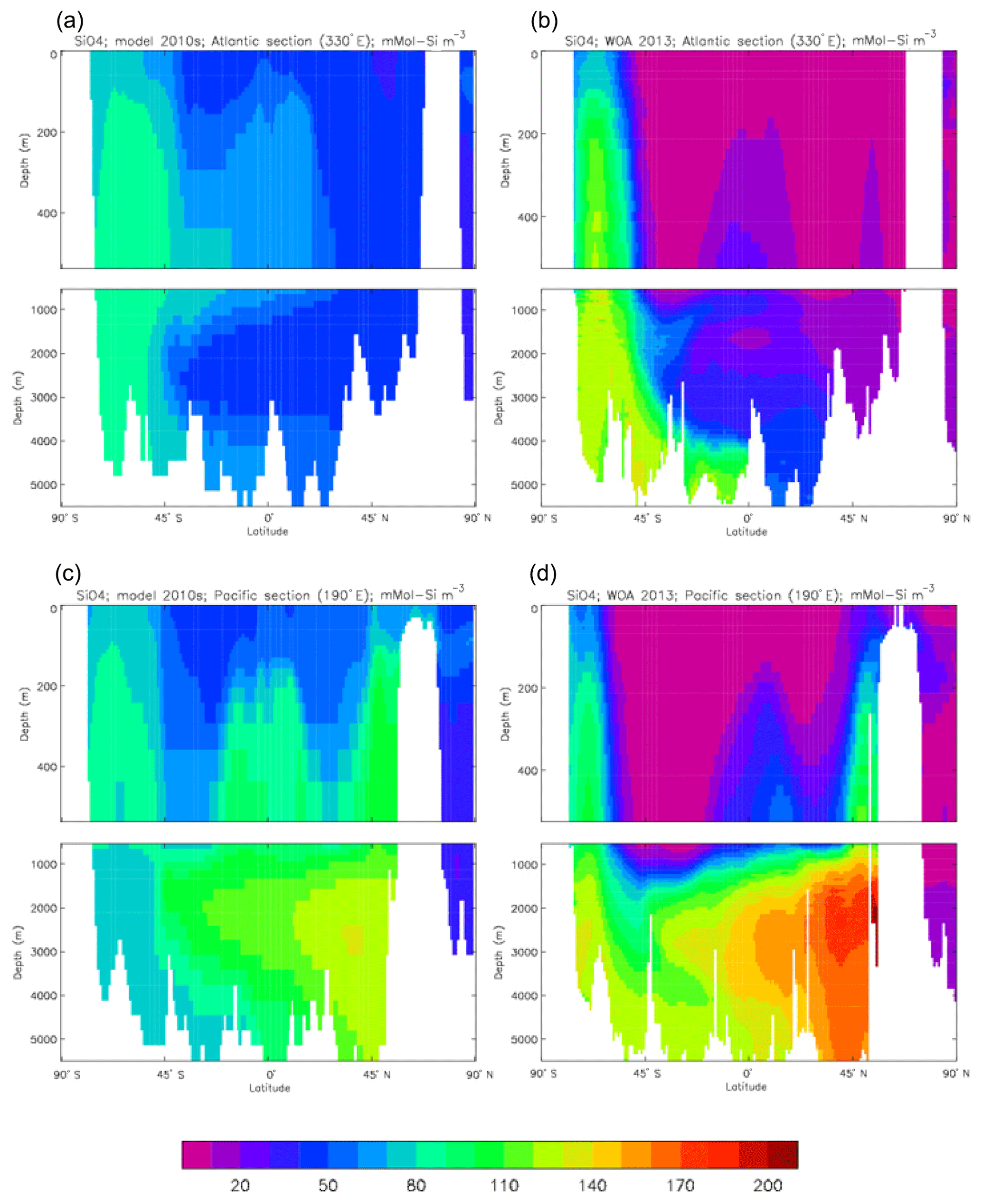
Figure 26Meridional sections of dissolved silicate (mMol Si m−3): panels (a) and (b) show sections in the Atlantic Ocean along 330∘; (c, d) Pacific Ocean sections along 190∘. Panels (a) and (c) show model concentrations averaged over 2010–2019; panels (b) and (d) show concentrations from the 2013 World Ocean Atlas gridded field.
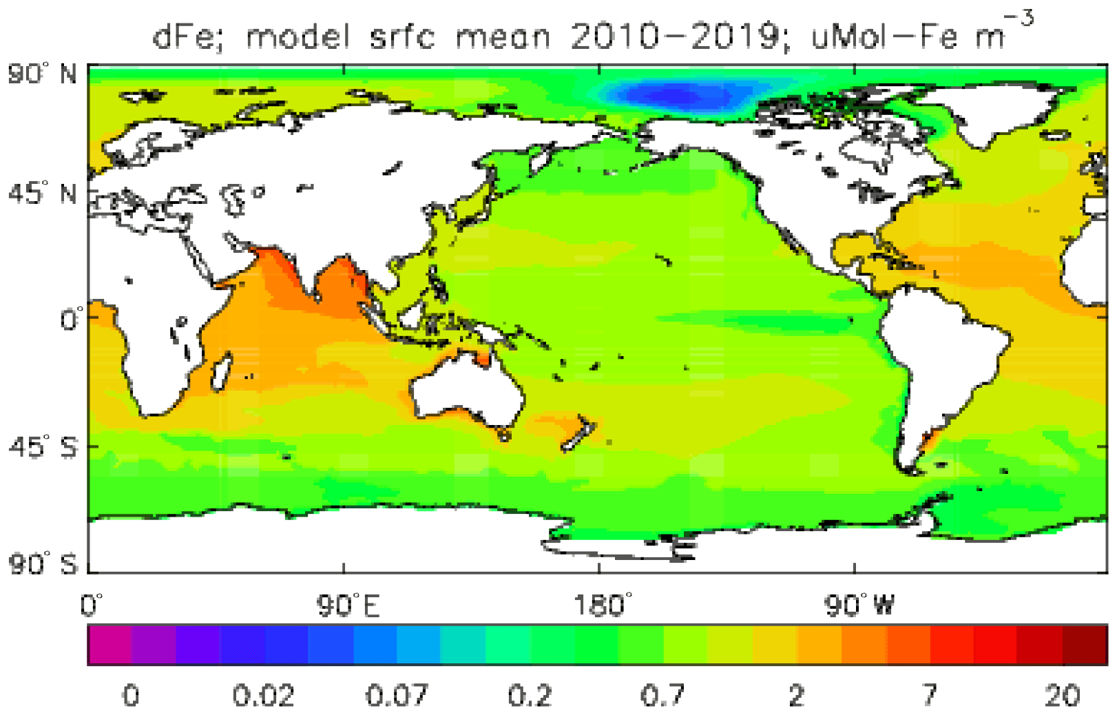
Figure 27Surface dissolved iron, averaged over model years 2010–2019 (µmol Fe m−3).
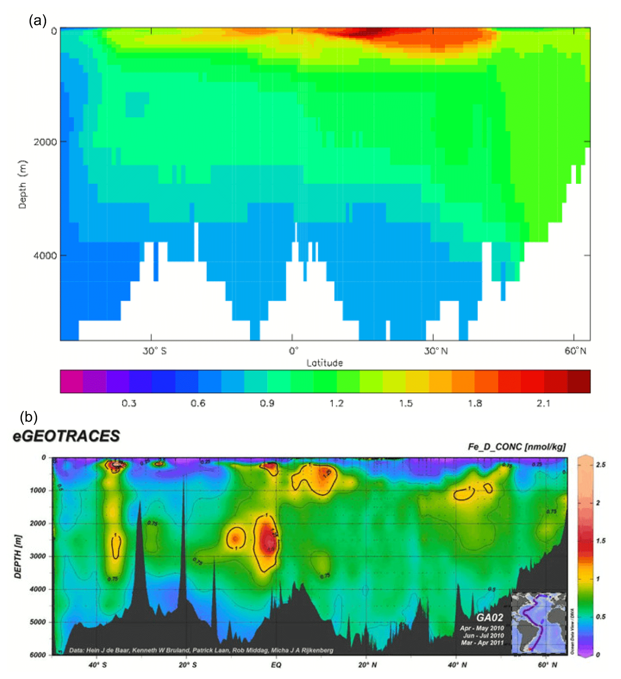
Figure 28Sections of dissolved iron (µmol Fe m−3) along the eGEOTRACES GA02 transect (in the Atlantic Ocean): (a) model concentrations averaged over the years 2010 to 2019; panel (b) is reproduced from eGEOTRACES.
4.1.9 Nutrients: nitrate, silicate, iron
Figure 22 compares the model surface nitrate field (mean over the years 2010 to 2019) with the corresponding field from Volume 4 of the World Ocean Atlas 2013 (hereafter WOA13V4; Garcia et al., 2014). Strictly the model nitrate field represents the sum of all dissolved inorganic nitrogen compounds (nitrate, nitrite and ammonium) but in many circumstances the first of those is dominant. Nitrogen is the “currency” of the model ecosystem and the main limiting nutrient. To 1st order the geographical distributions compare fairly well, with high concentrations in the Southern Ocean, the eastern equatorial Pacific, and the northern subpolar regions of the Pacific and Atlantic Ocean. The gridded data from WOA13V4 are slightly higher than the model in the eastern equatorial Pacific and in the subpolar North Atlantic; in the former region this is due to higher production in the model than is observed in the real ocean taking up more nitrate for phytoplankton growth, while in the latter the lower-than-observed production is due to low nitrate concentrations at the start of the growing season, in turn due to a tendency of the model to lose nutrient from that region through the deep circulation. It can also be seen that in the model the nitrate concentration has slipped to be slightly negative in some subtropical regions, particularly the centres of the gyres; in such circumstances the ecosystem model (but not the advection or mixing processes of the physical model) treats the value as zero. As shown in Fig. 29 (solid green square), the correlation of the decadal mean of the model and the gridded data is 0.96, while the ratio of the standard deviations is 1.01; note that to make these comparisons the gridded data were re-gridded to the model grid. Figure 23 compares full-depth meridional sections of the nitrate concentration in the Pacific and Atlantic Ocean (at 190 and 330∘, respectively) from the model and WOA13V4; the upper 500 m is shown with an expanded vertical scale. In the Atlantic sections, the model fails to simulate the northward intrusion of nitrate-rich water at around 1000 m of depth and its subsequent upwelling under the tropics; this is due to weak formation of Antarctic Intermediate Water, a know issue of the physical model. Also, in the model high northern latitudes, the nitrate concentration is much lower than the data at all depths, and the deficit is clearly carried with the North Atlantic Deep Water at depth to tropical and even high southern latitudes. This inability to retain high nutrient levels in the subpolar Atlantic has been seen in previous versions of the model (both physical and biogeochemical) and may be partially due to the absence of riverine inputs of nutrients into the Arctic Ocean and the high northern latitudes. In the Pacific section the comparison is better, though the model lacks the very high nitrate concentrations revealed in the WOA13V4 data at around 1000 m of depth north of 30∘ N. Figure 29 (open green square) shows that at around 1050 m of depth globally the correlation of the model and data is 0.89 and the ratio of the standard deviations is 1.30 (i.e. the model varies more). Figure 24 compares the amplitude and phase of the seasonal cycle in the model and WOA13V4 nitrate fields, determined by the best-fitting sine curve as described in previous sections; as in earlier figures of this type, the value of the amplitude and phase is only shown when the variance of the residual seasonal cycle is less than half that of the original cycle, determined separately for model and data fields. The seasonal cycle will be determined by a number of factors, including vertical advection and mixing and the uptake and remineralisation of nitrate by the ecosystem, all of which can vary through the year. The most obvious feature is that, while the seasonal cycle at most locations in the model (at both high and low latitudes) is well represented by a sine curve, there are far fewer locations in the gridded data for which this is so, and they are mainly at high latitudes (and particularly in the Northern Hemisphere). Where comparison can be made the model amplitude field is similar in pattern and scale to the mean concentration as presented in Fig. 22, but the WOA13V4 field shows some interesting differences from its concentration field: the scale of the seasonal cycle is much lower in the Southern Ocean (0.5 to 5 mMol N m−3 amplitude compared to greater than 20 mMol N m−3 mean, while the model has an amplitude of 5 to 15 mMol N m−3 with a similar mean). This suggests that the model is not fully limiting the phytoplankton growth in that region: this limitation will not be from low nitrate levels, as they are always higher than needed for growth, but could be from other nutrients (probably dissolved iron; see Martin, 1992) or from light limitation. In terms of the phase of the cycle, the model shows much greater consistency than WOA13V4: almost all the areas poleward of 30∘ in the model show the highest concentration at the end of local winter, but the data product shows much more variability in the Southern Hemisphere (both models show variability in the tropics). In Fig. 29, the Taylor diagram shows (in green) the correlations and ratios of the standard deviations of the midpoints (circle), amplitudes (upward-pointing triangle) and phases (downward-pointing triangle) of the best-fitting sine curves to the seasonal cycles of the model and data; the data have been re-gridded to the model's grid, and only points for which the sine curve is an acceptable fit are considered in the analysis. The midpoint, amplitude and phase have correlations of 0.94, 0.49 and 0.63, respectively, while the ratios of the standard deviations are 1.00, 1.54 and 0.90.
Figure 25 compares the model silicate field (i.e. dissolved silicic acid; meaned over the years 2010–2019) with the corresponding gridded field from WOA13V4. Unfortunately, the dissolution–remineralisation parameter for sinking detrital silicate was given a value that was too high; this meant that too much returned to dissolved silicate in the upper water column, leaving too little in the lower water column. Over the period of the simulations, therefore, the surface concentration of dissolved silicate continually increased (while that in the deep ocean continually decreased), leading to high surface values everywhere. This has the effect that, while it would normally be expected that silicate values will be low enough to limit the growth of diatoms (which require it to form their shells) in some areas all the time and in others at certain times of the seasonal cycle (after a bloom, for instance), in these model simulations silicate is never a limiting nutrient for diatoms, which are therefore only limited by nitrate, iron and light availability. Atlantic and Pacific Ocean meridional sections (at 330 and 190∘, respectively) in Fig. 26 show how the implementation error has raised the concentration throughout the upper water column in both oceans. Additionally, the Pacific section shows that the strong build-up of silicate in the North Pacific below 1000 m (and especially around 2000 m of depth) that is seen in WOA13V4 is not simulated to the same extent in the model. The Taylor diagram in Fig. 29 shows (red symbols) the correlations and ratios of the standard deviations of the surface annual mean concentration (filled square, correlation 0.69, ratio 0.64), annual mean concentration at 1050 m (open square, 0.78, 0.62), and the midpoint (circle, 0.64, 0.76), amplitude (upward-pointing triangle, 0.70, 0.36) and phase (downward-pointing triangle, 0.64, 0.89) of the best-fitting sine curve to the seasonal cycle. The data have been re-gridded to the model grid for this calculation and in the case of the best-fitting curve only those points with a good fit are considered. Although the silicate is too high across the ocean (as discussed) its seasonal cycle is strongly influenced by nitrogen- and light-limited diatom growth, so there is value in comparing it to the observations.
Figure 27 presents the surface dissolved iron concentration in the model, averaged over the years 2010 to 2019; the effects of high inputs of iron-rich dust can be seen in the northern subtropical Atlantic (from the Sahara), in the northern Indian Ocean (from the Arabian Peninsula and the Indian subcontinent) and east of Australia; most of the iron that is supplied to the surface layers of the Southern Ocean is upwelled or mixed from below. Given that the half-saturation concentration for iron limitation in both types of phytoplankton was set at 0.2 µmol Fe m−3, it can be seen that in the model there are few areas of the ocean where the decadal mean concentration of dissolved iron limits the growth of either misc-phyto or diatoms. However, there are significant areas, including the Southern Ocean, the eastern equatorial Pacific and the North Pacific, where iron is limiting at certain times of the seasonal cycle, though even this is different from the observed situation in which, for instance, iron is limiting in the Southern Ocean at all times of the seasonal cycle. Figure 28 compares the model to observations along a roughly meridional section in the western Atlantic Ocean. The data were collected for the eGEOTRACES GA02 transect (Schlitzer, 2019), and the model section follows the exact same path. The units in panel (a) (model) are micromoles of iron per cubic metre (µmol Fe m−3), while those in panel (b) (data; from http://www.egeotraces.org/sections/GA02_Fe_D_CONC.html, last access: 18 October 2019) are nanomoles of iron per kilogramme of seawater (nMol Fe kg−1); since the model's seawater density is set at 1025 kg m−3 (other than for calculations of density and pressure gradients, of course) these units are roughly comparable (2.5 % different, and it can be seen that the differences between the fields are considerably larger than that!). The model shows high concentrations in the surface water (due to strong atmospheric inputs), while the observations show low concentrations there. In contrast, the eGEOTRACES section (which mainly follows the shelf break) has a number of high-concentration patches well below the surface, which presumably are caused by dissolved iron being released from shelf-edge and basin margin sediments (which the model lacks). Analysis of the long-term behaviour of the dissolved iron field in the piControl simulation shows a drift to higher concentrations at all depths, including the surface levels, due to parameter values in the iron sub-model not being optimal and this field not being fully spun up. There is still much uncertainty in the quantitative understanding of the processes affecting iron in the ocean, especially those relating to organic ligands, and the representation used here can surely be improved.
4.1.10 Oxygen and apparent oxygen utilisation
Dissolved oxygen is present in the model (Eq. 5) as a diagnostic tracer. It has particular value as a diagnostic of the respiration of organic matter at depth in the water column but also allows for the simulation of oxygen minimum zones and their evolution under climate change. The surface oxygen concentration is not shown, since it is dominated by the temperature-dependent physical solubility process, but Fig. 30 compares the Atlantic and Pacific Ocean meridional sections (at 330 and 190∘, respectively). In both sections the overall patterns are very similar, with similar concentrations persisting in the model's plume of North Atlantic Deep Water as seen in the data (the gridded field from WOA13V4). The major difference is that the model's oxygen minimum concentrations are not as low as in the data: in the Atlantic around 130 mMol O2 m−3 compared to around 70 mMol O2 m−3 and in the Pacific around 70 mMol O2 m−3 below the tropics compared to as low as 20 mMol O2 m−3 below the subtropics in the data. This discrepancy could be due to the model having too little remineralisation in the relevant depth ranges or having too much mixing (of higher-oxygen water into the minimum zone). To assess the extent, geographically and vertically, of the low-oxygen regions, Fig. 31 compares the depth range of the water column with dissolved oxygen concentrations of less than 50 mMol O2 m−3 (panels a, b) and 100 mMol O2 m−3 (panels c, d) in the model (panels a, c) and WOA13V4 (panels b, d). The model almost exclusively produces such zones in the equatorial Pacific (particularly the eastern part of that), whereas WOA13V4 additionally shows oxygen-depleted water in the North Pacific and in the northern Indian Ocean. In the equatorial Pacific, however, the thicknesses of the low-oxygen zones are comparable in the model and data. In the Taylor diagram in Fig. 29 the blue symbols refer to oxygen variables: the filled square refers to the annual mean surface concentration (correlation 0.99, standard deviation ratio 1.01), the open square to the mean concentration at 1050 m (0.86, 0.96), the filled star to the thickness of the below-50 mMol O2 m−3 zone (0.30, 0.61) and the open star to the thickness of the below-100 mMol O2 m−3 zone (0.57, 0.87).
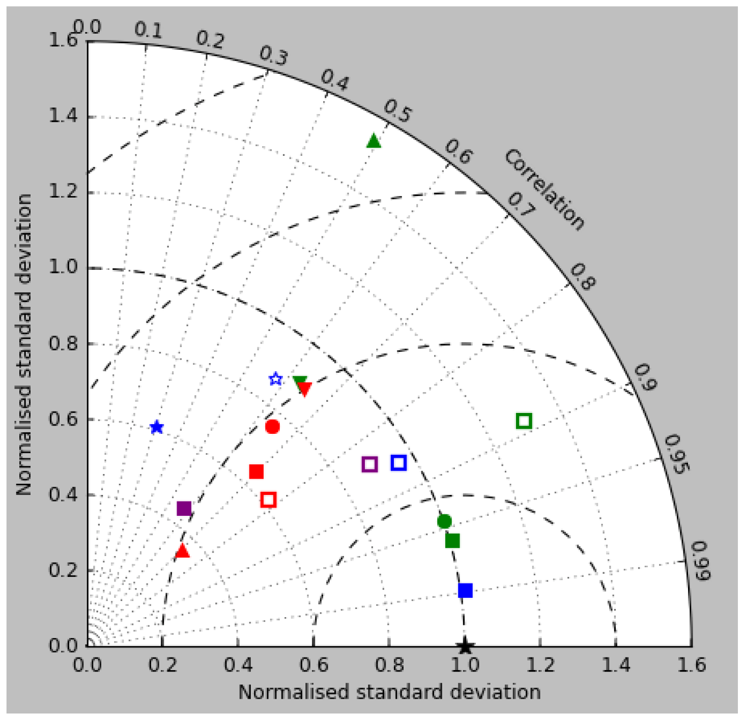
Figure 29Taylor diagram of nitrate (green), silicate (red), oxygen (blue) and apparent oxygen utilisation (purple); model values are averaged over the years 2010 to 2019, and observations are from the 2013 World Ocean Atlas. Filled squares show the surface concentrations, open squares the concentrations at the nearest depth level to 1050 m, and circles, upward-pointing triangles and downward triangles respectively show the midpoint, amplitude and phase of the sine curve that best fits the seasonal cycle (only at points for which the residual variance is less than half the original). The filled and open stars respectively show the vertical extent of the water column where the O2 concentration is below 50 and 100 mMol O2 m−3.
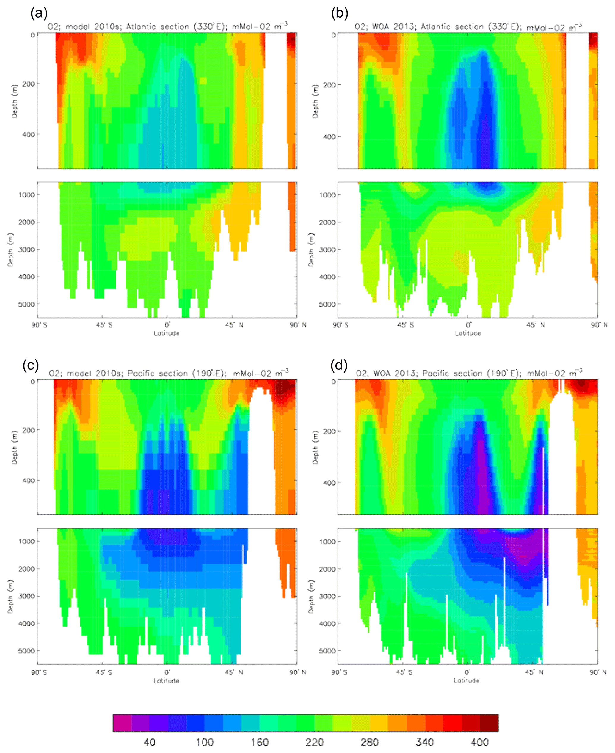
Figure 30Meridional sections of dissolved oxygen (mMol O2 m−3): panels (a) and (b) show sections in the Atlantic Ocean along 330∘; (c, d) Pacific Ocean sections along 190∘. Panels (a) and (c) show model concentrations averaged over 2010–2019; panels (b) and (d) show concentrations from the 2013 World Ocean Atlas gridded field.
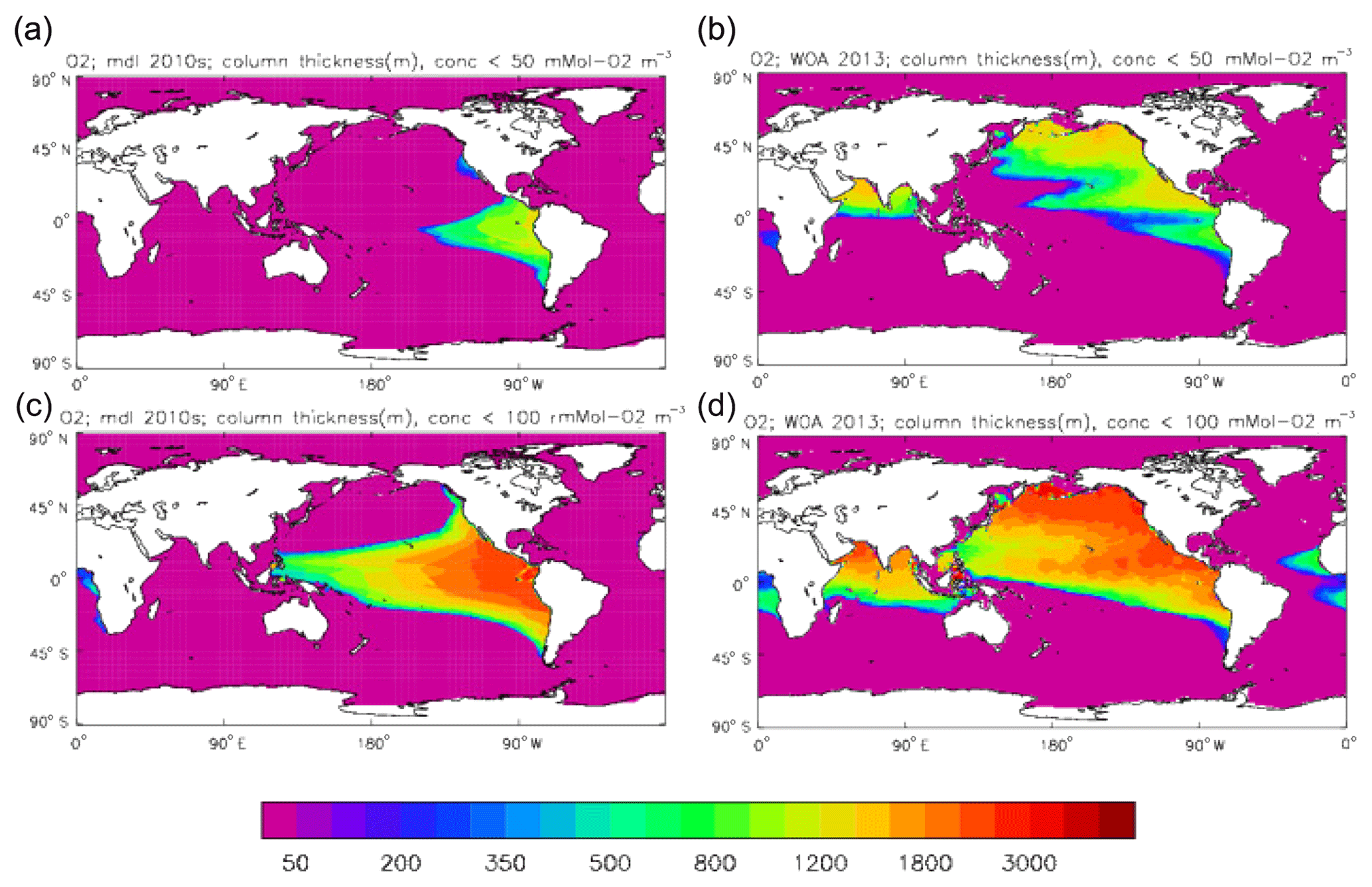
Figure 31Thickness (m) of the oxygen depletion zone in the water column; (a, c) from the model (averaged over the years 2010 to 2019), (b, d) from the 2013 World Ocean Atlas. Panels (a, b) and (c, d) show the extent of the water column in which O2 concentrations are below 50 and 100 mMol O2 m−3, respectively.
The apparent oxygen utilisation (AOU; mMol O2 m−3) is the difference between the oxygen solubility and the actual oxygen concentration in a water sample, and it is a measure of the accumulated biological activity in that sample since it was last at the surface (and in contact with the atmosphere). Values tend to be low (and negative) at the surface where oxygen-producing photosynthesis dominates but significantly higher in deeper, poorly ventilated water in which there has been much respiration. Figure 32a compares the geographical distribution of AOU at around 1050 m of depth in the model and in the gridded data (WOA13V4). The model matched the data over much of the ocean but significantly underestimates the value in the Indian Ocean and in the North Pacific; in the latter the model shows the highest values in the mid-latitudes (particularly on the eastern side of the basin), while the observed AOU increases northwards from the Equator and peaks in the northeast Pacific. The failure of the model to simulate extreme values at 1000 m of depth under the North Pacific has already been seen in the DIC, total alkalinity and nitrate sections. Figure 33 compares meridional sections of the model's AOU to the gridded GLODAPv2 field in the Atlantic Ocean (panels a, b; along 330∘) and in the Pacific Ocean (panels c, d; along 190∘). The simulation of the Atlantic section is mostly excellent, except for a slight underestimate at about 500 m of depth around 20∘ N, but the model misses the high values under the North Pacific as noted above; it can be seen that the error extends from 1000 to 3000 m of depth. In the Taylor diagram in Fig. 29 the purple symbols refer to AOU; the filled square refers to the surface value (correlation 0.57, standard deviation ratio 0.45) and the open square to the value at 1050 m of depth (0.84, 0.89), the mismatch in the latter being mainly due to the failure to simulate the high North Pacific and Indian Ocean values.
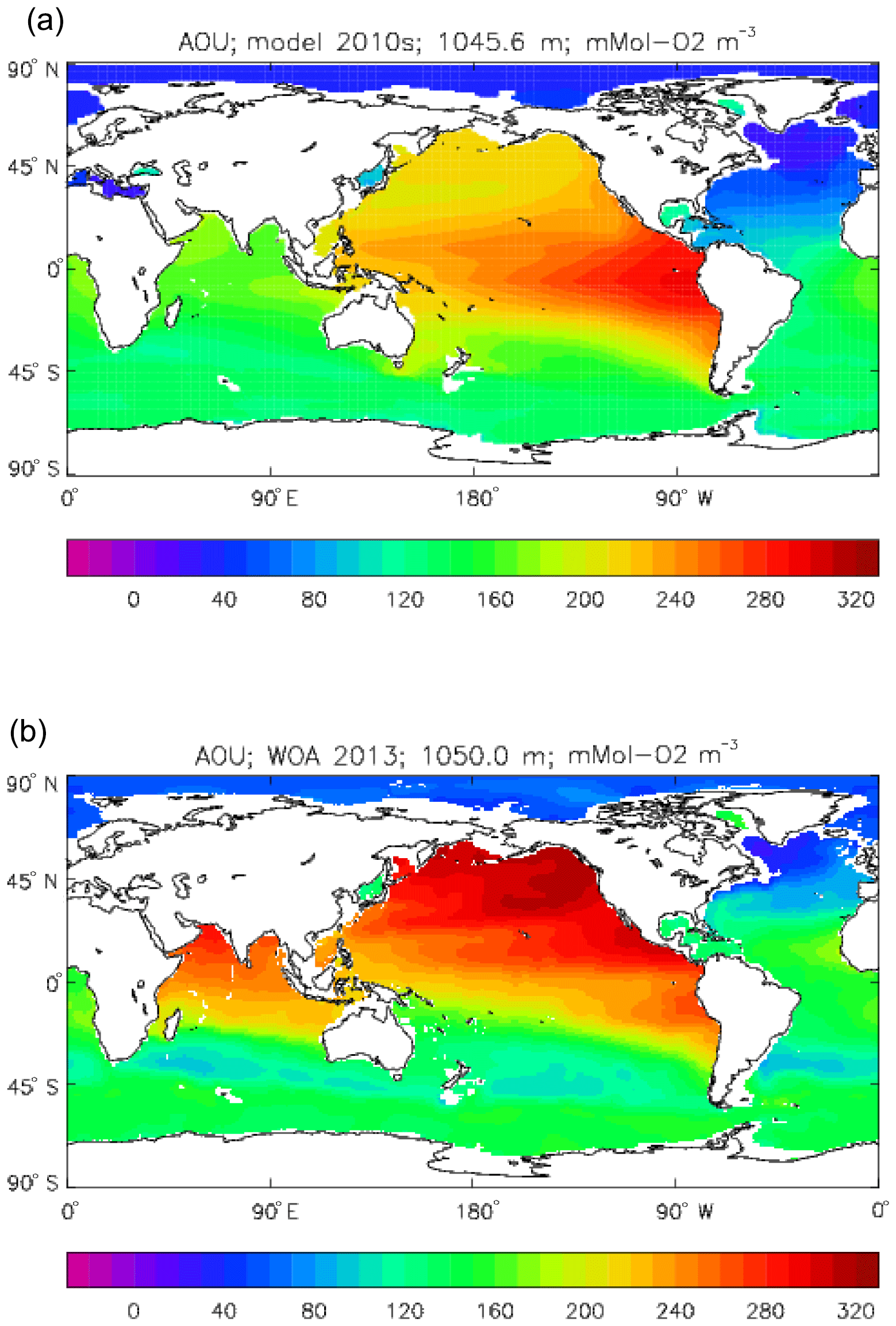
Figure 32Apparent oxygen utilisation (mMol O2 m−3): (a) model field at 1045.6 m, averaged over the years 2010 to 2019; (b) field at 1050 m from the 2013 World Ocean Atlas.
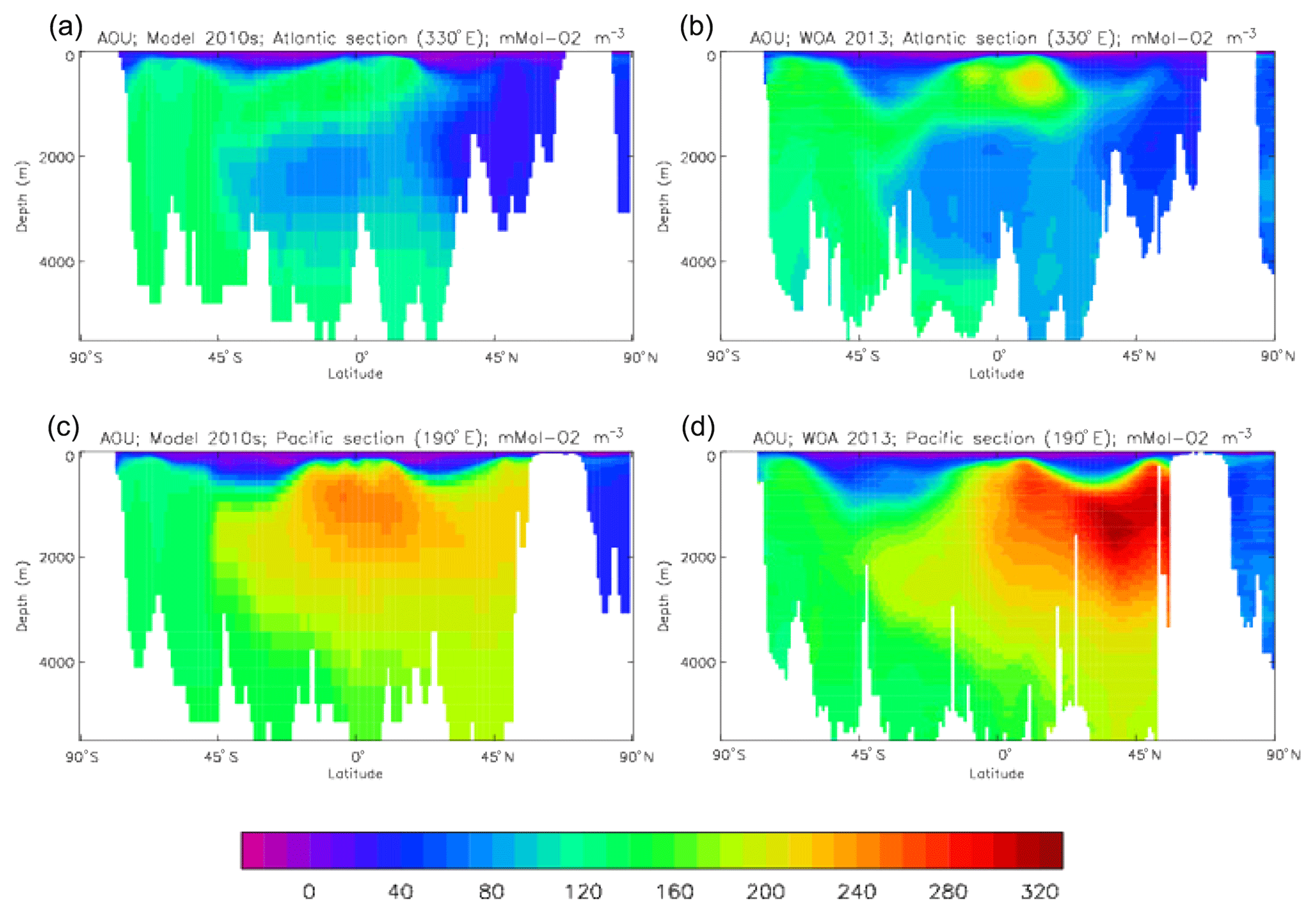
Figure 33Meridional sections of apparent oxygen utilisation (mMol O2 m−3): panels (a) and (b) show sections in the Atlantic Ocean along 330∘; (c, d) Pacific Ocean sections along 190∘. Panels (a) and (c) show model concentrations averaged over 2010–2019; panels (b) and (d) show concentrations from the 2013 World Ocean Atlas gridded field.
4.2 Response to climate change
This section presents key results of the response of the model to climate change in the RCP8.5 scenario simulation, in particular between the decade 2010–2019 (“the 2010s”) and the decade 2090–2099 (“the 2090s”), and also through the historical simulation from which the future run is initialised.
Figure 34 shows the global zonal mean surface nitrate concentration through the historical and RCP8.5 scenario period (years 1860 to 2099), allowing trends to be identified. The corresponding period of the piControl simulation (not shown) has no trend or drift, so the changes with time seen in this plot are all due to climate change. It can be seen that at almost all latitudes the concentration decreases through the 21st century and that the rate of decrease becomes more marked towards the end of the simulation. This trend can be understood in terms of the vertical supply of nitrate being reduced as the surface ocean is warmed and becomes more stratified. Although phytoplankton growth (and nitrate uptake) is also reduced because of the reduced nutrient availability, the net effect is a decrease in the surface nitrate concentration, and this drives many of the changes seen in the model and presented in this section.
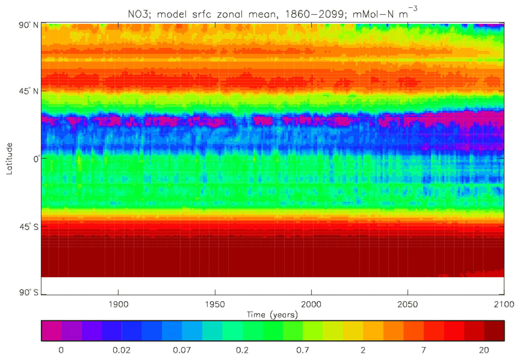
Figure 34Surface dissolved nitrate concentration (mMol N m−3): global zonal and annual means for model years 1860 to 2099 from the CMIP5 historical and RCP8.5 simulations, showing the response to changing climatic forcing.
Figure 35 presents Hovmöller plots of the total chlorophyll anomaly (a measure of the abundance of both types of phytoplankton) from 1860 to 2099 for the Atlantic basin (panel a) and the Pacific basin (panel b). The anomaly has been calculated by subtracting the chlorophyll in the piControl simulation (the mean from 1860 to 2099) from the annual mean chlorophyll in the historical+RCP8.5 simulation. The piControl chlorophyll showed no significant trend or drift. In addition to inter-annual and inter-decadal variability in both basins, it can be seen that trends become apparent in the climate change scenario, mainly after the year 2000. In both basins the chlorophyll close to the Antarctic continent increases substantially, as does that in the Atlantic basin around 45∘ S. In contrast, there is a clear reduction in chlorophyll at the Equator, which is present in both basins but particularly marked in the Pacific. Between 30 and 60∘ N there is a smaller reduction in chlorophyll in each basin, while in the Pacific just north of that band there is a marked increase. These trends can be understood as increased stratification both reducing the vertical nutrient supply and reducing the depth of the mixed layer during the growing season (and so improving the available light for phytoplankton in the surface layer): in the tropics the former dominates so production (and chlorophyll) is reduced, but at high latitudes the latter is more important and leads to higher production. In addition, around Antarctica warming seas mean that ice cover is reduced, allowing more primary production. Similar results have been reported previously in future scenario simulations (e.g. Bopp et al., 2001).
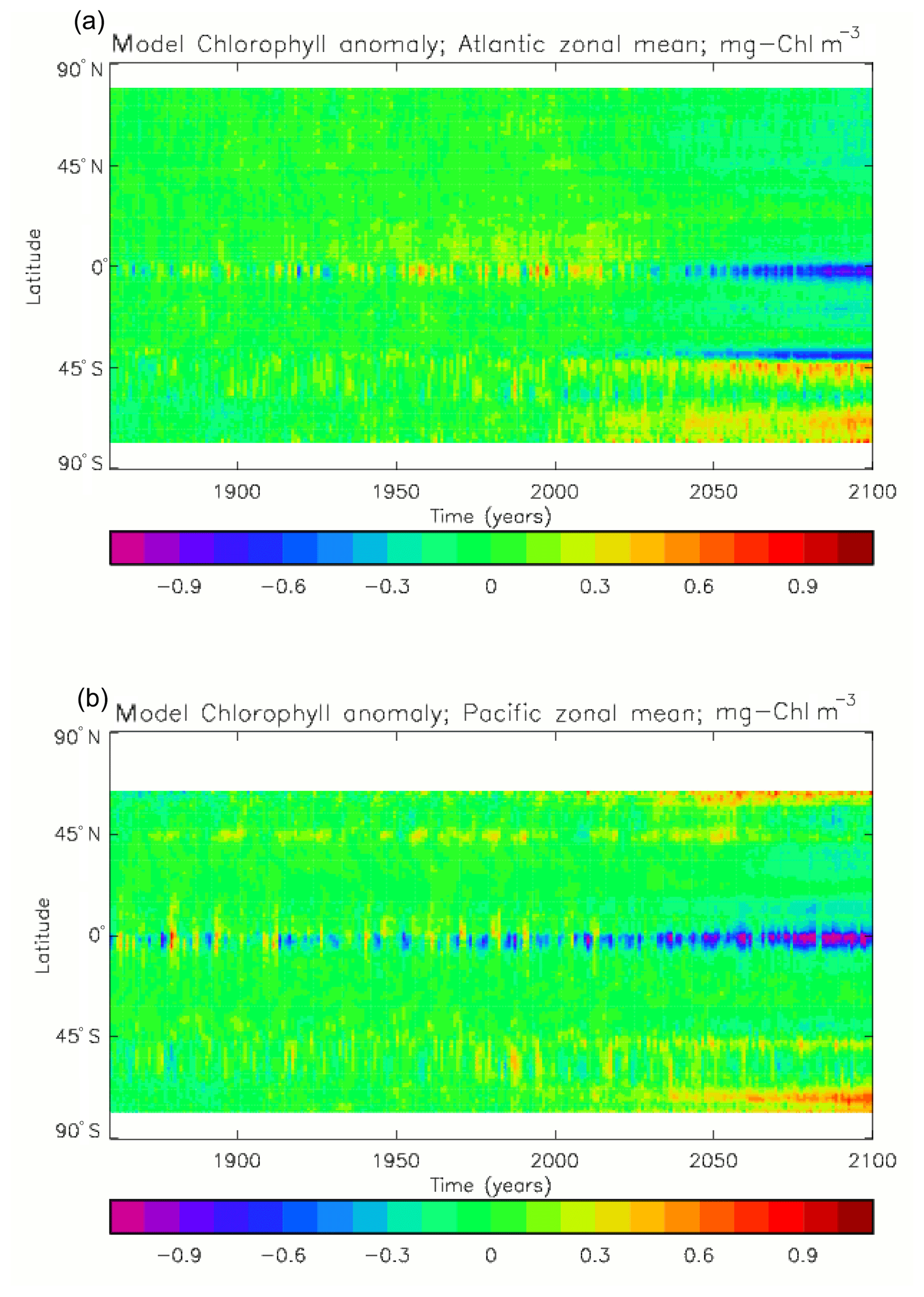
Figure 35Surface total chlorophyll concentration anomaly (mg Chl m−3), zonal and annual means for model years 1860 to 2099 from the CMIP5 historical and RCP8.5 simulations: (a) zonal mean of the Atlantic Ocean basin; (b) zonal mean of the Pacific Ocean basin. The anomaly has been calculated by subtracting the surface chlorophyll concentration field, meaned over the years 1860 to 2099, as produced by the piControl simulation from the annual means of the historical and RCP8.5 simulations.
Figure 36 shows how the seasonal cycle of total chlorophyll changes from the 2010s to the 2090s in the Atlantic basin (panel a) and the Pacific (panel b). In both basins the reduction in chlorophyll at equatorial latitudes is seen to be present throughout the year, though it is most intense in the Atlantic between July and November and in the Pacific during March and April. In the Southern Ocean sectors of each basin the change is an increase between October and February in the most southerly latitudes and no change in other months; however, slightly further north, around 45∘ S, there is an increase during those austral summer months in the Atlantic but a decrease in the Pacific. In the Northern Hemisphere, poleward of 40∘ N, the Atlantic sees a reduction between April and September but the Pacific sees a strong increase in the spring (March to May) followed by an equally strong reduction in the summer (June to August). This “dipole” change in the North Pacific is a signature of the seasonal cycle shifting forward by several months in response to changing physical conditions.
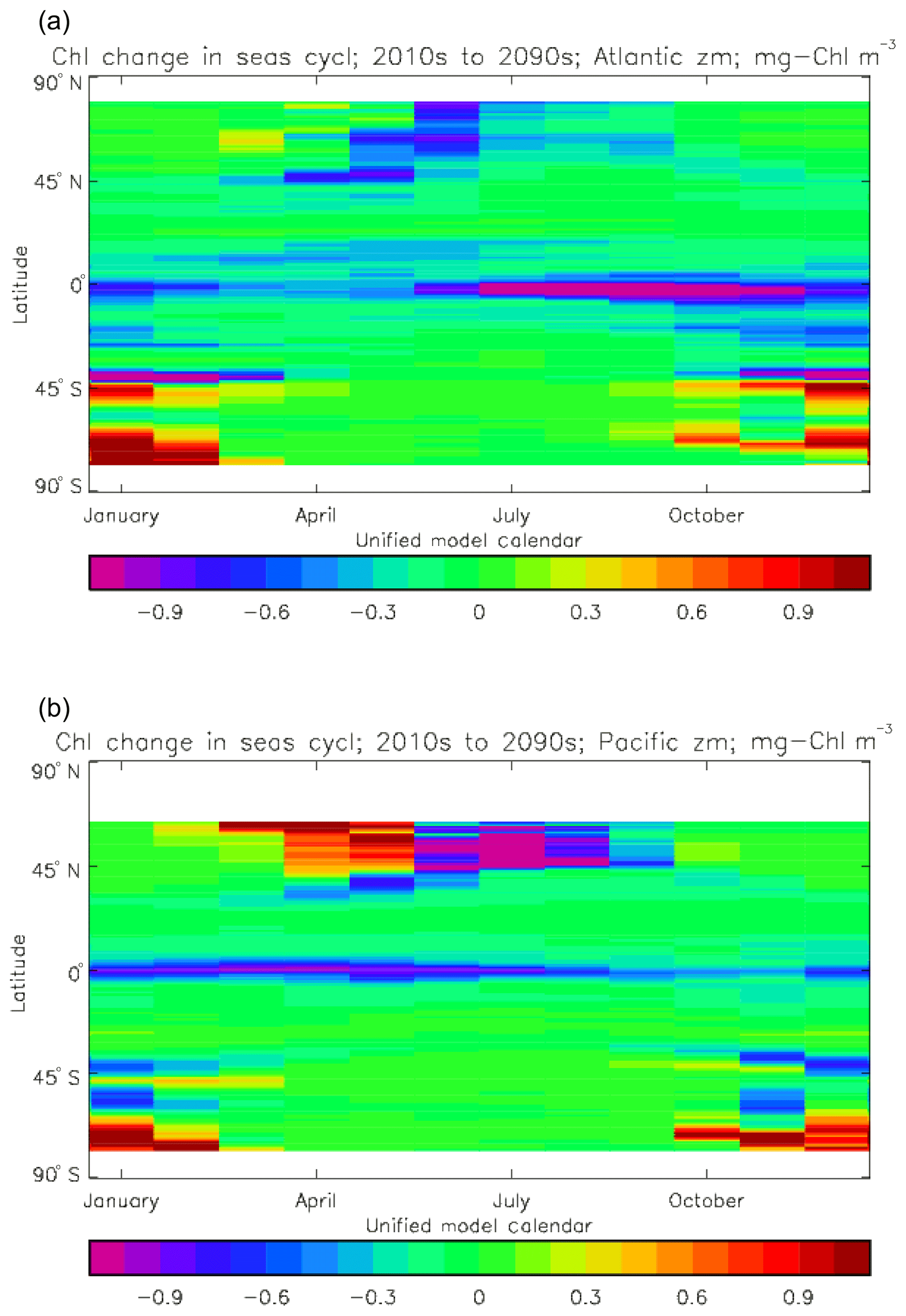
Figure 36Change in the seasonal cycle of surface chlorophyll concentration in the CMIP5 RCP8.5 simulation: change is calculated between the mean seasonal cycles of the model years 2090–2099 and 2010–2019. Zonal means of the (a) Atlantic Ocean basin and (b) Pacific Ocean basin.
Figure 37 shows the difference, between the 2090s and the 2010s, in the mean total primary production (panel a) and in the mean seasonal cycle of that quantity (panel b). The mean field displays strong reductions in the equatorial Pacific and Atlantic Ocean because of reduced nitrate availability and also in the subpolar North Atlantic and the eastern subpolar North Pacific. In contrast, the Southern Ocean close to the Antarctic continent shows strong increases in production for the reasons outlined above: shallower surface mixed layers, allowing the phytoplankton to remain longer in well-lit depths near the surface, and reduced seasonal ice cover, allowing more time for growth. The seasonal cycle shows a pattern of changes that is very similar to the change in the mean, except in the eastern equatorial Pacific where the amplitude of the cycle is little changed but the mean has been substantially reduced; note that in the 2010s the seasonal cycle was also relatively small, while the mean was high in that area. Figure 38 shows the change through time of the total production, separated into the Atlantic and Pacific basins (panels a and b, respectively). There are similarities as well as some differences between basins: both show a poleward spread (and consequently a slight overall increase) of production in the Southern Ocean, and both show a reduction in equatorial production through the 21st century; however, while the Northern Hemisphere subpolar production shows a marked decrease in the Atlantic basin throughout the last 100 years, no such change is seen in the Pacific (and there are hints of a slight increase). The global annual mean total primary production in the 2090s is 30.494 Pg C yr−1 (compared to 35.175 Pg C yr−1 in the 2010s, so a 13.3 % reduction), of which 17.227 Pg C yr−1 (cf. 19.791; −13.0 %) is apportioned to the diatoms and 13.267 Pg C yr−1 (cf. 15.384; −13.7 %) to the misc-phyto; therefore, there is only a very small shift towards increased dominance by the diatoms. Bopp et al. (2005) saw a decrease in the prevalence of diatoms under a warming scenario, and the opposite result obtained in this study is due to the lack of silicate limitation, which means that the diatoms are not prevented from utilising their higher growth rate; in fact, because the upwards drift in surface silicate concentrations is ongoing throughout the period of the future scenario, the silicate is less limiting in the future rather than more limiting as would be expected with increased stratification.
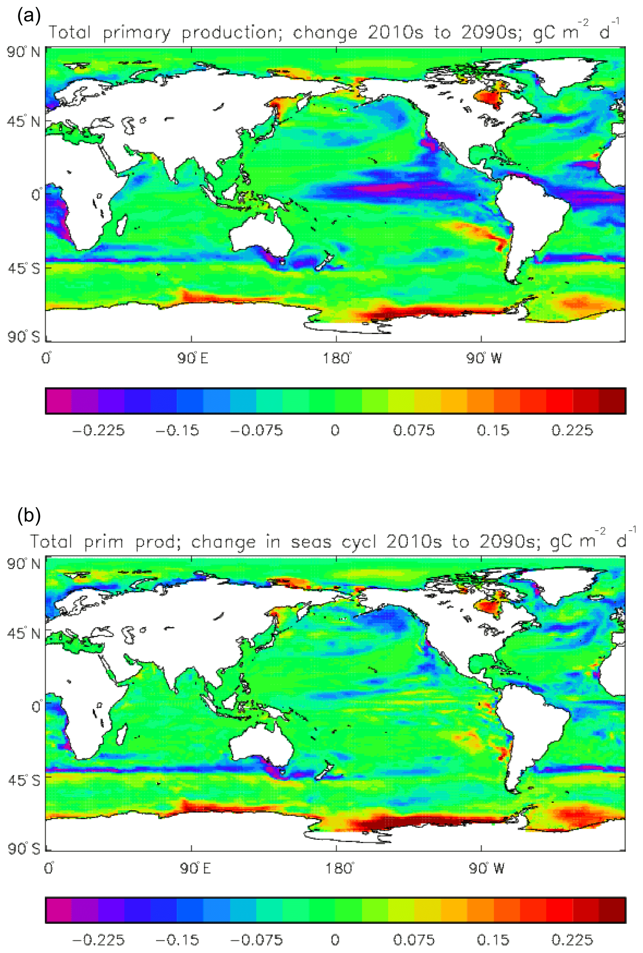
Figure 37Change in the depth-integrated total primary production (mg C m−2 d−1) in the RCP8.5 simulation: difference between the model years 2090–2099 and 2010–2019. (a) Difference in decadal means; (b) difference in the amplitude of the mean seasonal cycle.
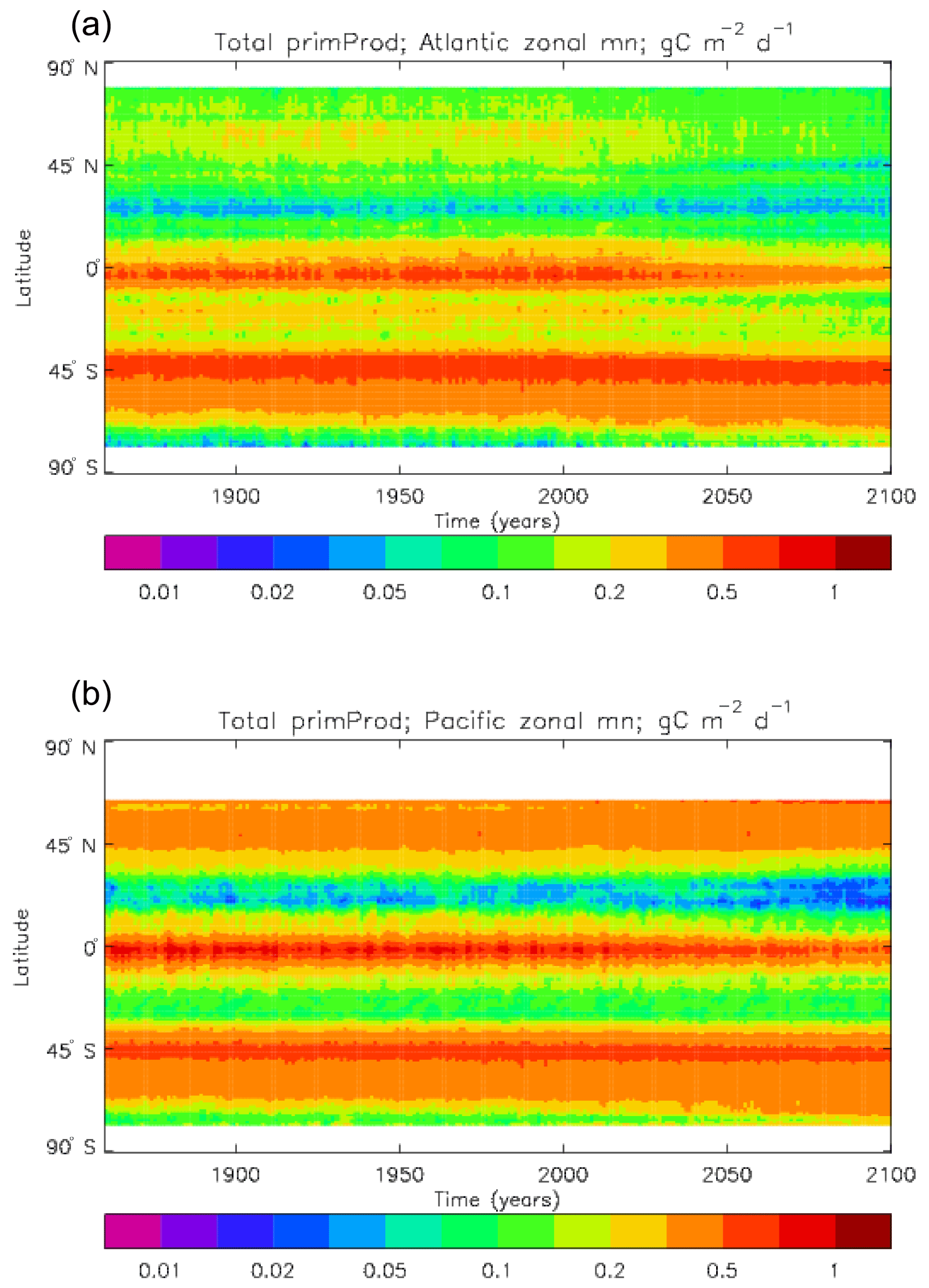
Figure 38Change in annual mean depth-integrated total primary production (g C m−2 d−1) during the model years 1860 to 2099 in the CMIP5 historical and RCP8.5 simulations. (a) Atlantic Ocean basin zonal mean; (b) Pacific Ocean basin zonal mean.
Figure 39 shows how the surface ocean pCO2 varies through the historical and RCP8.5 scenario. Figure 39a shows the change with time of the global zonal mean pCO2 anomaly (i.e. the difference between the scenario and the piControl). As expected, the surface pCO2 increases smoothly with time, increasing its rate in keeping with the prescribed atmospheric concentration. Most of the rise therefore occurs during the 21st century. It is notable that all latitudes increase at a substantially similar rate. Figure 39b shows the geographical distribution of the anomaly averaged over the period 2090–2099. Here the colour scale has been set to show what differences there are: the rise is greatest in the Arctic, in the subtropical gyres and in the northern subpolar Atlantic. Figure 39c shows that the distribution of the anomaly of the seasonal cycle amplitude is very similar to that of the mean concentration, except around the Antarctic continent. The phase of the seasonal cycle in the 2090s (not shown) has changed little from that in the 2010s.
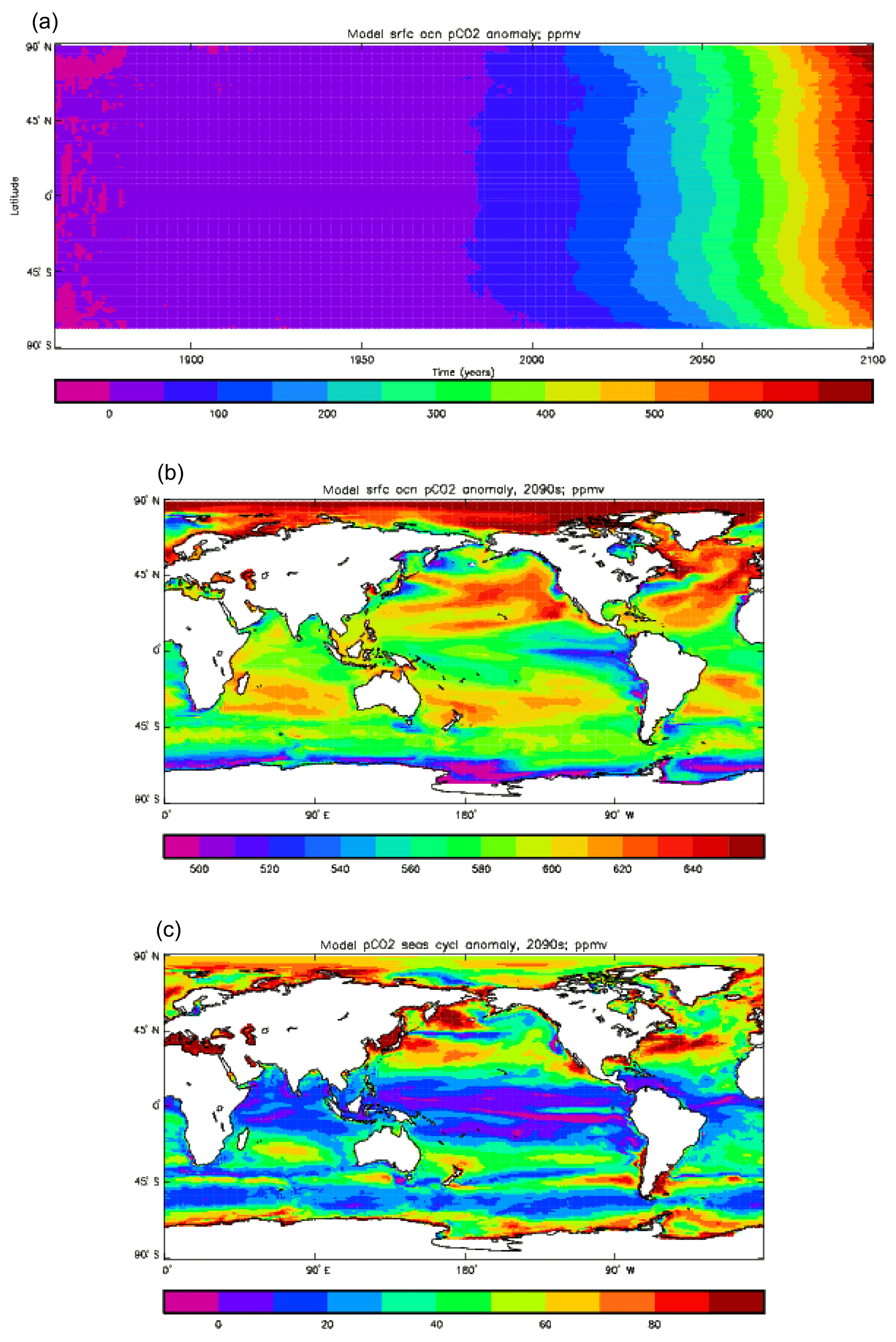
Figure 39Change in surface pCO2 (ppmv) during the model years 1860 to 2099 in the CMIP5 historical and RCP8.5 simulations. (a) The anomaly over the period of the simulations, calculated by subtracting the annual means of the piControl simulation from those of the historical and RCP8.5 simulations. (b) The decadal mean anomaly during the model years 2090–2099, calculated by subtracting the relevant years of the piControl from those of the RCP8.5 simulation. (c) The seasonal cycle amplitude anomaly averaged over the model years 2090–2099, calculated as for panel (b).
Finally, the air-to-sea flux of CO2 is considered. Figure 40 shows the global total flux through the historical+RCP8.5 simulation from 1860 to 2099 (the piControl over that period showed no trend). It is clear that the flux increases with time; this is to be expected, since the atmospheric pCO2 was increasing monotonically through the simulation. By the 2090s the net flux is 4.8 Pg C yr−1.
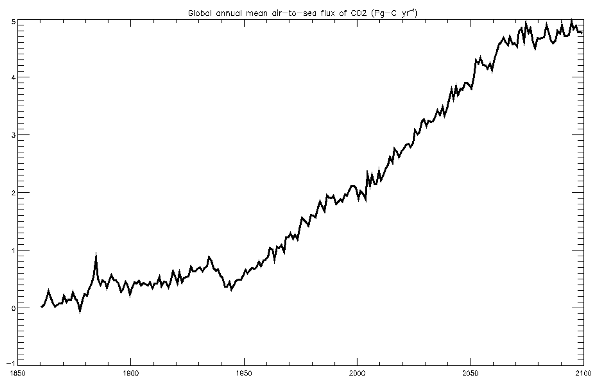
Figure 40Time evolution of the annual mean global total air-to-sea CO2 flux (Pg C yr−1) between model years 1860 and 2099 in the CMIP5 historical and RCP8.5 simulations.
Figure 41 shows the evolution of the zonal mean flux globally (panel a) and in the Atlantic and Pacific basins separately (panels b and c, respectively). It can be seen that, while the global total flux continued to increase throughout the period, there were certain latitudes in some basins where the flux peaked and then began to decline – despite the atmospheric CO2 concentration continuing to increase. This effect is particularly noticeable in the Atlantic between 50 and 60∘ N, with the peak uptake occurring between 1980 and 2030 before an accelerating decrease. Such a “peak and decline” feature is seen in many CMIP5 model simulations as well as in other future simulations, and the causes are examined in Halloran et al. (2015). In the Southern Ocean, meanwhile, the uptake shows a monotonic and significant increase, particularly in the second half of the 21st century.

Figure 41Change in the annual mean total air-to-sea CO2 flux (ng C m−2 s−1) during model years 1860 to 2099 in the historical and RCP8.5 simulations. (a) Global zonal mean; (b) Atlantic Ocean basin zonal mean; (c) Pacific Ocean basin zonal mean.
Figure 42 shows the seasonal cycle of the zonally meaned total flux during the 2090s globally and in each ocean basin separately. It can be compared to Fig. 20, which shows the same cycles during the 2010s. It is clear that there has been a substantial shift towards net uptake, particularly where there was already substantial uptake in the 2010s; but there are some areas which were sources at the earlier time that became sinks for atmospheric CO2 at the later time. There are also regions (e.g. the Atlantic around 45∘ N) which were weak sources in the summer months during the 2010s but which have become strong sources by the 2090s; this is despite those latitudes being stronger sinks in the winter and spring months at the later time. Overall, therefore, the cycling of CO2 between the ocean and atmosphere seems to have generally intensified. This result is consistent with the conclusions of Hauck and Völker (2015), who argued that, due to a reduction in the Revelle (or buffer) factor of the surface waters, the seasonal cycle due to biological growth will become relatively more important.

Figure 42The seasonal cycle (monthly means) of the total air-to-sea CO2 flux (ng C m−2 s−1) averaged over the model years 2090–2099. Zonal mean of (a) global ocean, (b) Atlantic Ocean basin, (c) Indian Ocean basin, (d) Pacific Ocean basin.
The Diat-HadOCC model is a development of the earlier HadOCC model, including separate diatom and misc-phytoplankton components and representations of the dissolved silicate and iron cycles in the ocean and through the marine ecosystem. The model forms the ocean biogeochemistry component of the Met Office's coupled Earth system model HadGEM2-ES and has been used to run a wide-ranging suite of simulations for the CMIP5 experiment. This paper has described the model in detail, presenting the equations and explaining choices made in the parameterisations. The Diat-HadOCC model's performance has been evaluated by comparing a selection of results from the CMIP5 simulations to publicly available data products such as the World Ocean Atlas 2013 and GLODAPv2. The model results shown (and many more) are freely available from the Earth System Grid website (https://esgf-node.llnl.gov/, last access: 18 October 2019).
The model has been shown to be capable of reproducing to a reasonable extent many of the important features of the marine carbon cycle, including annual mean surface concentrations of dissolved inorganic carbon, total alkalinity and the annual air–sea flux of CO2. However, there are also significant differences from the real-world observations in these quantities, both in the surface layer (where the effect on the air–sea CO2 flux is direct) and in the deep and mid-waters (where model errors will take decades to centuries to affect that flux). Some of these differences may be due to errors in the physical ocean model's deep circulation, but some will be due to errors in the ecosystem performance. The climate change response of the marine carbon cycle in the model is also shown to be in accordance with similar modelling studies.
In terms of the ecosystem, the model does less well. The model's total chlorophyll (the sum of diatom chlorophyll and misc-phytoplankton chlorophyll) is too high in many areas (by a factor of 2 or more), including in the eastern equatorial Pacific and the Southern Ocean, while being lower than observed in the oligotrophic gyres. In contrast, the model's primary production (global mean 35.2 Pg C yr−1) is slightly below the range estimated from observations, even when the highly productive coastal regions are ignored (the physical structure of the model means those regions will not be adequately represented). Therefore, the model produces too much chlorophyll that does not do enough. The split between diatoms and misc-phytoplankton is roughly even, with the former having 55 % of the biomass and being responsible for 56 % of the primary production. The geographical distributions of the two phytoplankton types are also very similar, and this similarity is roughly maintained even under the RCP8.5 climate change scenario. The reason for the two types being so similar is due to many of their parameters having the same values (an exception is the maximum growth rate, which is higher for diatoms) and due to the dissolved silicate and dissolved iron fields not being limiting to diatom growth as much as they should be. The dissolved nitrate field is represented fairly well, though its surface concentration is low in the North Atlantic due to circulation issues (and a lack of riverine inputs). The dissolved silicate field, by contrast, suffers from a poor choice of the detrital silicate dissolution parameter, which leads to a drift to excessively high surface values through the run and so is rarely limiting. Surface concentrations of dissolved iron, which should be limiting in most areas of the ocean for at least some of the year, are also too high because the iron in the particulate biology is remineralised too shallow in the water column. The iron sub-model is not a success and is discussed below, whereas the silicate problem, not being due to any inherent flaw in the model structure or equations, can be corrected by choosing a more suitable (i.e. lower) value for the relevant parameter.
The iron sub-model was developed for the Diat-HadOCC model (and so for use in HadGEM2-ES) at a time (circa 2007) when much less was known about the cycling of iron through the ocean ecosystem. This was particularly the case for a quantitative understanding of the system, which is required to produce a predictive numerical model. It is not enough to know that a certain process happens; in order to include it successfully in an Earth system model the rate at which it happens and how it depends (or not) on temperature and other factors (including concentrations of state variables) has to be known. It is certainly the case that if the Diat-HadOCC model was being developed now the iron sub-model would be very different from the one used as part of HadGEM2-ES in the CMIP5 experiments. In particular, the forced remineralisation of all iron at the point at which material enters the detrital compartment(s) would not be repeated: there is incontrovertible evidence (Boyd et al., 2017) that iron is found in sinking detrital particles, and even in the model the problem that the choice was pragmatically made to address – too little iron in the surface waters – has ceased to exist since subsequent changes to the land-surface scheme in HadGEM2-ES led to increased dust deposition to the ocean and so a greater surface iron supply. The result in the simulations was that the surface iron concentration was too high and was rarely limiting to phytoplankton growth.
One innovation used in the Diat-HadOCC model relates to how various phytoplankton and zooplankton processes respond to iron stress. Originally suggested by the late Professor Mike Fasham based on unpublished work, it provides separate iron-replete and iron-deplete parameter values, with the realised value at any time and location being determined by the dissolved iron concentration. The intention was to provide an effective shortcut when a quantitative mechanistic understanding of how iron affects certain biological processes is lacking or when an accurate representation would require extra state variables (e.g. for internal pools of stored nutrients). The model allows five processes to be modified this way: the growth rate of diatoms, the growth rate of misc-phytoplankton, the Si:N ratio for uptake by diatoms, the preference for zooplankton feeding on diatoms and the natural mortality of zooplankton. The last two are not meant to suggest that dissolved iron directly affects any individual zooplankton, or indeed any particular zooplankton species, in that way but rather recognises that the single zooplankton compartment used in the Diat-HadOCC model has to necessarily represent an assemblage of different zooplankton species, and iron stress will lead to diatoms being more heavily silicified and so affect the relative palatability of diatoms as prey and the make-up of that assemblage. In a different model that has two zooplankton state variables, it might be possible to produce such a shift in the assemblage more explicitly, and so it might not be necessary to use that last shortcut. The success of this innovation was not fully tested in the CMIP5 experiments, as the iron-replete and iron-deplete parameter values were set to be equal in all except the case of diatom growth rate. The decision to do that was taken after a limited sensitivity analysis showed no great benefits in making the values significantly different, and it was reasoned that, as just part of a much larger ESM running predictive simulations over several hundred years, it was better to “play it safe” and err on the side of caution when there was no strong reason to do otherwise.
The problems of the too-high surface dissolved silicate and dissolved iron concentrations, while scoring poorly on some ocean ecosystem metrics, do not invalidate the air–sea flux of CO2 or the ocean carbon storage in the simulated results submitted to the CMIP5 experiment. The effect of those too-high concentrations is to make the diatom phytoplankton state variable not limited by silicate and iron and so behave more similarly to the misc-phytoplankton state variable than it should; therefore, the total primary production and carbon drawdown are like what would be seen if there was a single phytoplankton state variable limited only by dissolved inorganic nitrogen (and light). While such a single-phytoplankton ecosystem model would lack some of the climate responses that it was hoped the Diat-HadOCC model would explore, it would still be a valid model, so the representation of the wider carbon cycle (including the ocean carbon cycle) is not impaired. It is a disappointment that the Diat-HadOCC model as implemented for the CMIP5 experiments was not able to fully explore the intended range of potential feedbacks (e.g. changes in iron limitation due to changes in dust deposition, the effect of changes in the relative abundance of the two phytoplankton types). However, this failing was largely due to cautious choices of certain parameter values, which led to the phytoplankton types being very similar in behaviour, and poor choices of others, which led to the drift in surface dissolved silicate concentrations; with different parameter choices the model structure and equations could explore those potential feedbacks. The main structural problems concern the iron sub-model, in particular the forced remineralisation of iron rather than letting it become part of sinking detritus, and in light of significant research undertaken since the model was developed this sub-model would benefit from being significantly changed.
The Diat-HadOCC model took part in the comparative study (Kwiatkowski et al., 2014) to choose the ocean biogeochemical sub-model for the first UK Earth system model (UKESM1), but it was not chosen. In light of that decision there are no plans to develop the Diat-HadOCC model further. However, this paper achieves the important task of giving a detailed description of the Diat-HadOCC model that was used as part of HadGEM2-ES to run simulations for the CMIP5 experiment, which informed the 5th Assessment Report of the IPCC and as such is a valuable record. Certain parameterisations uniquely used by the model have been highlighted. The successes and weaknesses of the model have been presented and discussed, making it clear when the latter are due to the model structure and when they are the result of parameter choices.
Due to intellectual property right restrictions, the author cannot provide either the source code or documentation papers for the Unified Model (UM). The Met Office Unified Model is available for use under licence. A number of research organisations and national meteorological services use the UM in collaboration with the Met Office to undertake basic atmospheric process research, produce forecasts, develop the UM code, and build and evaluate Earth system models. For further information on how to apply for a licence, see http://www.metoffice.gov.uk/research/modelling-systems/unified-model (last access: 18 October 2019).
The variation with light availability of the primary production of each phytoplankton type is calculated using the production scheme of Anderson (1993; hereafter TRA93). This models the preferential absorption of longer-wavelength light by seawater so that the spectrum of light available for growth is shifted towards blue deep in the euphotic zone. Note that consequently the light calculated and used for photosynthesis in these functions at a given depth will not be the same as that available to the physics (for heating): the physics could easily be made to use the biological light field but does not do so as standard (and did not in the CMIP5 simulations). The functions also integrate production over a day based on the noon surface irradiance and the number of daylight hours (from Eq. 5 of Platt et al., 1990). This is consistent with the once-daily frequency of atmosphere–ocean coupling used in HadGEM2-ES (and previously in HadCM3C) because daily average light is passed through the coupler and noon irradiance can easily be calculated given the daily average and the number of daylight hours (and assuming, as Platt et al., 1990, did, that the light varies sinusoidally within the daylight hours only). Note that although the light will stay the same for each time step between couplings the other factors determining production (e.g. phytoplankton abundance and nutrient concentration) will not, so the production is recalculated every time step and the appropriate proportion of daily production added to the phytoplankton state variable (e.g. 1∕24 for a 1 h time step). When the HadOCC model (which uses the same productivity model) has been forced by 6-hourly reanalysis fluxes, for example, a daily average irradiance field has been calculated and passed in for use in this scheme. When used in coupled models with shorter coupling periods, either a running 24 h average of irradiance could be calculated and the scheme used as designed (and as described in the following paragraphs), or the daily integral part of the scheme could be removed and instantaneous production calculated using the remainder of the scheme.
TRA93 built on earlier work by Morel (1988, 1991), which measured the absorption of light due to water and chlorophyll in 61 wavelength bands, each 5 nm wide, across the visible spectrum between 400 and 700 nm. Considering six typical chlorophyll depth profiles, TRA93 showed that the changing spectrum of light with depth (due to red light being more readily absorbed than blue) could be taken into account by splitting the water column into three depth ranges, allowing the absorption in each depth range to be modelled by a different function of the chlorophyll concentration. It was found that the best-fitting solution put the boundaries between the ranges at 5 and 23 m of depth, and the parameters for the three functions published in TRA93 related to those splits. However, since the physical ocean model in HadGEM2-ES (and also in previous Met Office GCMs, including HadCM3) has layer interfaces at 10 and 20 m the scheme was re-parameterised for depth-range boundaries at those depths, and the model described here uses those new values. Note, however, that in other implementations of the Diat-HadOCC model (e.g. Kwiatkowski et al., 2014) the original TRA93 parameter values are used; when a light-scheme boundary (at 5 or 23 m) falls within a model layer that model layer is split in two at the appropriate depth for the purposes of calculating the primary production, and the results from the two sublayers are then combined to update the phytoplankton biomass.
Using the notation of TRA93, the spectrally averaged vertical attenuation coefficient for layer n within depth range L, kn (m−1), is given by that paper's Eq. (16):
where cn is the square root of Gn, the total pigment concentration in layer n (mg m−3), and the re-parameterised coefficient values bi,L are given in Table A1. TRA93 assumed the chlorophyll biomass is always 80 % of the total pigment biomass G (the remainder being pheophytin), and the HadOCC and Diat-HadOCC models make the same assumption.
Table A1Polynomial coefficients relating k to the square root of pigment in depth range L.
Table A2Polynomial coefficients for as a function of pigment and depth.
Table A3Polynomial coefficients and rational function coefficients for psynth calculation.

A derived parameter a#, required to calculate light absorption by phytoplankton, is then calculated by finding its surface value (TRA93 Eq. 20) and integrating down the water column, being parameterised in terms of c and the depth z (TRA93 Eqs. 21–23). The paper's equations allow the pigment concentration to have a depth profile that varies continuously with depth, but as implemented in Met Office GCMs the concentration is taken as being constant within a model layer and changing suddenly at the depth interfaces. TRA93 showed that this requires an offset to a# when crossing between model layers: this offset is equal to the difference between calculated using the G for each layer.
The calculation (in layer n) of the model variable astarn, which corresponds to a# in TRA93, is performed layer by layer, stepping down from the surface; the value is calculated at the midpoint of each layer:
where astar1 is the model variable corresponding to TRA93's , astar00=astar01 and corresponds to , dastar1 corresponds to integrated over depth from the top to the bottom of layer 1 and where the following equations apply.
In the above equations is the carbon-to-chlorophyll ratio (mgC mgChl−1), which is either calculated according to Eq. (B1) or fixed, wC is the molecular weight of carbon, 12.01 mg mol−1, and Zn is the depth (in metres) of the base of layer n, with Z0=0.0 m. Note that the gcof coefficients relate to the g coefficients in TRA93's Eqs. (18) and (21) but are numbered in a different order, as shown in Table A2; in TRA93 they were ordered by the total exponent of c and ν combined, but the Diat-HadOCC model (like the HadOCC model) orders them by the exponent of ν.
Based on TRA93's Eq. (29) (itself derived from work described in Platt et al., 1990) the primary production for each phytoplankton type (Dm or Ph) in layer n during a whole day can then be calculated using a fitted 5th-order polynomial. In that equation, a quantity shown as is calculated; Platt et al.'s polynomial is fitted for values of that quantity between 0.0 and 15.8 and the fitted function oscillates wildly outside that range, but in the model the value of the corresponding quantity can be larger than 15.8. Therefore, a rational function with non-oscillatory behaviour was calculated (Geoff Evans, personal communication, 1993) which matches the 5th-order polynomial at an input of 15.8 in both value and first derivative, and this is used for higher input values. For phytoplankton type X and layer n (of thickness Δn), the following equations apply.
The values of the coefficients Ω and γ are given in Table A3. In the above equations, is the maximum photosynthetic efficiency ( in TRA93) and has the value 2.602 times αX, the initial slope of the photosynthesis–light curve (Eq. 26 in TRA93). is the maximum growth rate for the phytoplankton type and layer, taking into account the temperature and nutrient limitations, as calculated in Eqs. (10) and (11); solbio0 is the solar radiance just below the ocean surface. The total daily production in that layer is then
where dlh is the number of daylight hours at that location and time of year, and k is the attenuation coefficient calculated in Eq. (A1). All terms in these equations (except dlh and the constant π) vary between layers. Where a number of layers are part of a surface mixed layer at a given time step the production in those layers is averaged over those layers.
The carbon-to-chlorophyll ratio for each phytoplankton type, , can either be prescribed or updated using a scheme based on Geider et al. (1996, 1997, 1998). In the CMIP5 simulations run using HadGEM2-ES, the constant values shown in Table B1 were used. However, for completeness the time-varying scheme as implemented in the Diat-HadOCC model is described briefly.
Rearranging Eqs. (A1)–(A5) in Geider et al. (1997; hereafter G97) produces (using that paper's notation, including , so corresponding to the reciprocal of the ratio used in this model)
where G97's corresponds to this model's PX, αchl corresponds to , I is the irradiance (in the middle of the layer), and Rchl and RC are respectively the specific removal rates of chlorophyll and carbon from the phytoplankton. Finally, kchl is the “maximum proportion of photosynthesis that can be directed to chl a synthesis” but in a number of conditions is equal to the maximum (chl∕C) ratio, and in this model it is represented by . The equation above has no analytical solution for θ, and it is intended that the model should be able to operate with long time steps if required (up to 1 d), so a semi-implicit finite-difference solution was found. is represented as , and the θ inside the exponents takes the value θt (i.e. the reciprocal of the value of from the previous time step), while those outside take the value θt+1. RC is set equal to (where X is Ph or Dm as appropriate), and Rchl is set equal to RC (so the difference is zero). Then a simple rearrangement results in a quadratic equation in θt+1, which can be easily solved. The updated value of is then the reciprocal of the resulting θ (though it can be necessary on occasions to apply upper and lower bounds to the ratio: and , respectively). Ratios calculated in layers that are part of the surface mixed layer are averaged. As implemented, the ratio is stored from one time step to the next and not advected or mixed as a tracer; the change in the ratio due to biological processes is much larger than that due to mixing with the ratio in adjacent grid boxes. It would be possible to use the ratio and the concentration of the appropriate phytoplankton type to create a phytoplankton–chlorophyll state variable which could be advected and mixed as a tracer, but that is not how the scheme is currently used in the Diat-HadOCC model.
Finally, the calculations of the air-to-sea fluxes of O2 and CO2 ([Oxyasf] and [CO2asf], respectively) follow the methodology of OCMIP. The flux is the product of the gas-specific gas transfer (piston) velocity Vp and the difference between the gas concentrations in the atmosphere (just above the sea surface), Xsat, and in the (surface) ocean, Xsurf:
The piston velocity (m s−1) is a function of the 10 m wind speed, U (using the Wanninkhof 1992 formulation, normalised for a Schmidt number of 660), the gas-specific Schmidt number Sch and the fraction of the grid box area that is open water Aow:
where fU is a coefficient taking the value 0.31 if wind speed averaged over a day or less is used (e.g. in a coupled model) or 0.39 if monthly mean wind speed is used (Wanninkhof, 1992).
In the case of oxygen O2,surf is the model oxygen concentration, while the surface ocean is assumed to be fully saturated in equilibrium so O2,sat is equal to the solubility (mL O2 L−1; converted to model units before use). That is calculated using Eq. (8) of Garcia and Gordon (1992) but removing the spurious “” term found at the end of the first line (as in the o2sato.f subroutine in the OCMIP-2 Biotic-HOWTO documentation, available at http://ocmip5.ipsl.jussieu.fr/OCMIP/phase2/simulations/Biotic/boundcond/o2sato.f, last access: 18 October 2019). The solubility coefficients used in the OCMIP-2 subroutine, originally from Benson and Krause Jr. (1984) and recommended by Garcia and Gordon (1992), are used here. Note that in HadGEM2-ES the sea-level pressure is assumed to always be 1.0 atm. Therefore, the equation is
where sea-surface temperature T has units of degrees Celsius, salinity S has units of per mille and where . can be converted to units of moles of O2 per cubic metre (mol O2 m−3) by dividing by the molar volume, 22.3916 L mol−1. The Schmidt number is calculated according to Keeling et al. (1998):
where , protecting the calculation from crashing if the physical ocean model should produce unreasonably low or high sea-surface temperatures.
In the case of carbon dioxide , where is the CO2 solubility and pCO2,atm is the partial pressure of CO2 in dry air at 1 atm of pressure in the atmospheric level immediately above the ocean surface (note again that the sea-level pressure is always assumed to be 1 atm). The solubility is that from Weiss (1974):
where (protecting the calculation from any spuriously low sea-surface temperatures the physical model might produce). The Schmidt number for CO2 is calculated according to Wanninkhof (1992):
where Tl is defined as in the calculation for .
The calculation of CO2,surf has to take into account the partitioning of DIC into three forms, namely carbonic acid (taken here to include the dissolved gas phase), bicarbonate ion and carbonate ion, only the first of which contributes to the air-to-sea flux:
The calculation of the partitioning, which follows the method described by Bacastow (1981), requires as inputs the total alkalinity AT, the DIC concentration, the temperature, the salinity and the total boron concentration. The method involves using a term χx,i, which is dependent as shown in Eq. (C22) on an earlier estimate of the hydrogen ion concentration [H+] to calculate the carbonate alkalinity . AC is then used with DIC to set up a quadratic equation in the related term χy,i. Bacastow (1981) then used the secant method of similar triangles (Acton, 1970) to produce an updated estimate and to minimise the difference between successive estimates. This algorithm is explained in more detail below.
Four equilibrium constants describing the dissociation of carbonic acid (K1; from Roy et al., 1993), bicarbonate ion (K2; also from Roy et al., 1993), boric acid (KB; from Dickson, 1990) and water (KW; from Millero, 1995) are calculated (moles per kilogramme).
∘C is the temperature in Kelvin and S the salinity in per mille. Note that, because these constants are in units of moles per kilogramme of seawater (strictly, (moles per kilogramme of seawater)2 in the case of KW), the alkalinity and DIC state variables must be converted to those units from the model units of millimoles per cubic metre (mMoles m−3) before the partitioning is calculated; all state variables in the converted units have the subscript u (e.g. AT,u).
The total borate concentration BT (in moles per kilogramme) is set to be proportional to the salinity: . Then, since the Diat-HadOCC model uses the five-term expression for total alkalinity (Bacastow, 1981), the carbonate alkalinity is calculated as
where
Equations (C7) and (C16) can be rearranged and combined with Eqs. (C8), (C10), (C18), (C19) and (C22) to give a quadratic in χy,i:
which has the solution
If χy,i and χx,i are found to be equal, then their value gives the sought-after value of χ that is consistent with AC,u and DICu for the current temperature and salinity, and from that [H2CO3] can be found from Eqs. (C7), (C8) and (C10). But usually those two estimates of χ will not be equal, and then the secant method of similar triangles (Acton, 1970) is used to find an updated estimate for input into the next iteration of Eq. (C17) by minimising χy−χx. The two similar triangles are right-angled and have sides of length and , respectively; equating the ratios of these two triangles' sides and rearranging gives
This calculation can be iterated until the fractional change in successive estimates is less than a certain amount (e.g. 10−5). However, in the implementation used for HadGEM2-ES the calculation was iterated eight times; it had been found that the convergence criterion was always satisfied in six iterations, and given the computer architecture it was more computationally efficient to run that way than to repeatedly test for convergence.
Once the carbonic acid concentration has been determined (and converted back to model units) it can be used as CO2,surf in the air–sea flux calculation. Other diagnostic quantities can also be calculated: pCO2 and pH (the latter from the H+ concentration).
The author declares that there is no conflict of interest.
The development of the HadGEM2 family represents the work of a large number of people, to whom the author is indebted. The author also wishes to thank three anonymous reviewers for their perceptive and detailed comments which greatly helped to improve the paper.
This research has been supported by the Joint DECC/Defra Met Office Hadley Centre Climate Programme (grant no. GA01101).
This paper was edited by Guy Munhoven and reviewed by three anonymous referees.
Acton, F. S.: Numerical Methods that Work, Harper and Row, New York, 52, 1970. a, b
Anderson, T. R.: A spectrally averaged model of light penetration and photosynthesis, Limnol. Oceanogr., 38, 1403–1419, 1993. a
Antonov, J. I., Seidov, D., Boyer, T. P., Locarnini, R. A., Mishonov, A. V., Garcia, H. E., Baranova, O. K., Zweng, M. M., and Johnson, D. R.: World Ocean Atlas 2009, Volume 2: Salinity, in: NOAA Atlas NESDIS 68, edited by: Levitus, S., U.S. Gov. Printing Office, Wash., DC, 2010. a
Aranami, K. and Tsunogai, S.: Seasonal and regional comparison of oceanic and atmospheric dimethylsulfide in the northern North Pacific: Dilution effects on its concentration during winter, J. Geophys. Res., 109, D12303, https://doi.org/10.1029/2003JD004288, 2004. a
Bacastow, R. B.: Numerical evaluation of the evasion factor, in: Scope 16: Carbon cycle Modelling, edited by: Bolin, B., John Wiley, New York, 95–101, 1981. a, b, c
Benson, B. B. and Krause Jr., D.: The concentration and isotopic fractionation of oxygen dissolved in freshwater and seawater in equilibrium with the atmosphere, Limnol. Oceanogr., 29, 620–632, 1984. a
Best, M. J., Pryor, M., Clark, D. B., Rooney, G. G., Essery, R. L. H., Ménard, C. B., Edwards, J. M., Hendry, M. A., Porson, A., Gedney, N., Mercado, L. M., Sitch, S., Blyth, E., Boucher, O., Cox, P. M., Grimmond, C. S. B., and Harding, R. J.: The Joint UK Land Environment Simulator (JULES), model description – Part 1: Energy and water fluxes, Geosci. Model Dev., 4, 677–699, https://doi.org/10.5194/gmd-4-677-2011, 2011. a
Bopp, L., Monfray, P., Aumont, O., Dufresne, J.-L., Le Treut, H., Madec, G., Terray, L., and Orr, J. C.: Potential impact of climate change on marine export production, Global Biogeochem. Cy., 15, 81–99, 2001. a
Bopp, L., Aumont, O., Cadule, P., Alvain, S., and Gehlen, M.: Response of diatoms diatribution to global warming and potential implications: A global model study, Geophys. Res. Lett., 32, L19606, https://doi.org/10.1029/2005GL023653, 2005. a
Bopp, L., Resplandy, L., Orr, J. C., Doney, S. C., Dunne, J. P., Gehlen, M., Halloran, P., Heinze, C., Ilyina, T., Séférian, R., Tjiputra, J., and Vichi, M.: Multiple stressors of ocean ecosystems in the 21st century: projections with CMIP5 models, Biogeosciences, 10, 6225–6245, https://doi.org/10.5194/bg-10-6225-2013, 2013. a
Boyd, P. W., Ellwood, M. J., Tagliabue, A., and Twining, B. S.: Biotic and abiotic retention, recycling and remineralization of metals in the ocean, Nat. Geosci., 10, 167–173, https://doi.org/10.1038/NGEO2876, 2017. a, b
Boyd, P. W., Claustre, H., Levy, M., Siegel, D. A., and Weber, T.: Multi-faceted particle pumps drive carbon sequestration in the ocean, Nature, 568, 327–335, https://doi.org/10.1038/s41586-019-1098-2, 2019. a
Bryan, K.: A numerical method for the study of the circulation of the world ocean, J. Comput. Phys., 4, 347–376, 1969. a
Carr, M.-E., Friedrichs, M. A. M., Schmeltz, M., Aita, M. N., Antoine, D., Arrigo, K. R., Asanuma, I., Aumont, O., Barber, R., Behrenfeld, M., Bidigare, R., Buitenhuis, E. T., Campbell, J., Ciotti, A., Dierssen, H., Dowell, M., Dunne, J., Esaias, W., Gentili, B., Gregg, W., Groom, S., Hoepffner, N., Ishizaka, J., Kameda, T., Le Quéré, C., Lohrenz, S., Marra, J., Mélin, F., Moore, K., Morel, A., Reddy, T. E., Ryan, J., Scardi, M., Smyth, T., Turpie, K., Tilstone, G., Waters, K., and Yamanaka, Y.: A comparison of global estimates of marine primary production from ocean color, Deep-Sea Res. Pt. II, 53, 741–770, 2006. a
Clark, D. B., Mercado, L. M., Sitch, S., Jones, C. D., Gedney, N., Best, M. J., Pryor, M., Rooney, G. G., Essery, R. L. H., Blyth, E., Boucher, O., Harding, R. J., Huntingford, C., and Cox, P. M.: The Joint UK Land Environment Simulator (JULES), model description – Part 2: Carbon fluxes and vegetation dynamics, Geosci. Model Dev., 4, 701–722, https://doi.org/10.5194/gmd-4-701-2011, 2011. a
Coleman, K. and Jenkinson, D. S.: RothC-26.3: a model for the turnover of carbon in soil, in: Evaluation of soil organic matter models using existing, long-term datasets, edited by: Powlson, D. S., Smith, P., and Smith, J. U., NATO ASI Series I, Springer-Verlag, Heidelberg, 38, 237–246, 1996.
Coleman, K. and Jenkinson, D. S.: RothC-26.3, A model for the turnover of carbon in soil: Model description and Windows User's guide: November 1999 issue, Harpenden, UK, available at: http://www.rothamsted.ac.uk/sustainable-soils-and-grassland-systems/rothamsted-carbon-model-rothc, https://repository.rothamsted.ac.uk/item/8829q/rothc-26-3-a-model-for-the-turnover-of-carbon-in-soil-model-description-and-windows-users-guide-november-1999-issue (last access: 18 October, 2019), 1999.
Collins, W. J., Bellouin, N., Doutriaux-Boucher, M., Gedney, N., Halloran, P., Hinton, T., Hughes, J., Jones, C. D., Joshi, M., Liddicoat, S., Martin, G., O'Connor, F., Rae, J., Senior, C., Sitch, S., Totterdell, I., Wiltshire, A., and Woodward, S.: Development and evaluation of an Earth-System model – HadGEM2, Geosci. Model Dev., 4, 1051–1075, https://doi.org/10.5194/gmd-4-1051-2011, 2011. a, b
Cox, M. D.: A primitive equation, three dimensional model of the ocean, Ocean Group Tech. Rep. 1, GFDL, Princeton, NJ, USA, 143 pp., 1984. a
Cox, P. M.: Description of the TRIFFID Dynamic Global Vegetation Model, Hadley Centre Technical Note HCTN 24, Met Office, FitzRoy Road, Exeter EX1 3PB, UK, available at: http://www.metoffice.gov.uk/media/pdf/9/h/HCTN_24.pdf and https://digital.nmla.metoffice.gov.uk/ (last access: 18 October 2019), 2001. a
Cox, P. M., Betts, R. A., Jones, C. D., Spall, S. A., and Totterdell, I. J.: Acceleration of global warming due to carbon-cycle feedbacks in a coupled climate model, Nature, 408, 184–188, 2000. a
Dickson, A. G.: Thermodynamics of the dissociation of boric acid in synthetic seawater from 273.15 to 298.15 K, Deep-Sea Res., 37, 755–766, 1990.
Dukowicz, J. K. and Smith, R. D.: Implicit free surface method for the Bryan-Cox-Semtner ocean model, J. Geophys. Res., 99, 7991–8014, 1994. a
Eppley, R. W.: Temperature and phytoplankton growth in the sea, Fish. B-NOAA, 70, 1063–1085, 1972. a
Essery, R. L. H., Best, M. J., Betts, R. A., Cox, P. M., and Taylor, C. M.: Explicit representation of sub-grid heterogeneity in a GCM land-surface scheme, J. Hydrometeorol., 4, 530–543, 2003. a
Fanton d'Andon, O. H., Antoine, D., Mangin, A., Maritorena, S., Durand, D., Pradhan, Y., Lavender, S., Morel, A., Demaria, J., and Barrot, G.: Ocean colour sensors characterisation and expected error estimates of ocean colour merged products from GlobColour, Ocean Optics XIX, Barga, Italy, 51 pp., 6–10 October 2008.
Fasham, M. J. R., Ducklow, H. W., and McKelvie, S. M.: A nitrogen-based model of plankton dynamics in the oceanic mixed layer, J. Mar. Res., 48, 591–639, 1990.
Fasham, M. J. R., Flynn, K. J., Pondaven, P., Anderson, T. R., and Boyd, P. W.: Development of a robust marine ecosystem model to predict the role of iron in biogeochemical cycles: A comparison of results for iron-replete and iron-limited areas, and the SOIREE iron-enrichment experiment, Deep-Sea Res. Pt. I, 53, 333–366, https://doi.org/10.1016/j.dsr.2005.09.011, 2006. a
Ford, D. A., Edwards, K. P., Lea, D., Barciela, R. M., Martin, M. J., and Demaria, J.: Assimilating GlobColour ocean colour data into a pre-operational physical-biogeochemical model, Ocean Sci., 8, 751–771, https://doi.org/10.5194/os-8-751-2012, 2012. a, b, c
Garcia, H. E. and Gordon, L. I.: Oxygen solubility in seawater: Better fitting equations, Limnol. Oceanogr., 37, 1307–1312, 1992. a, b
Garcia, H. E., Locarnini, R. A., Boyer, T. P., Antonov, J. I., Baranova, O. K., Zweng, M. M., and Johnson, D. R.: World Ocean Atlas 2009. Volume 3: Dissolved Oxygen, Apparent Oxygen Utilization, and Oxygen Saturation, in: NOAA Atlas NESDIS 69, edited by: Levitus, S., U.S. Gov. Printing Office, Washington, DC, 2010a. a
Garcia, H. E., Locarnini, R. A., Boyer, T. P., Antonov, J. I., Baranova, O. K., Zweng, M. M., and Johnson, D. R.: World Ocean Atlas 2009, Volume 3: Dissolved Oxygen, Apparent Oxygen Utilization, and Oxygen Saturation, in: NOAA Atlas NESDIS 69, edited by: Levitus, S., U.S. Gov. Printing Office, Washington, DC, 2010b. a
Geider, R. J., MacIntyre, H. L., and Kana, T. M.: Dynamic model of phytoplankton growth and acclimation: responses of the balanced growth rate and the chlorophyll a:carbon ratio to light, nutrient limitation and temperature, Mar. Ecol. Prog. Ser., 148, 187–200, 1997.
Gent, P. R., and McWilliams, J. C.: Isopycnal mixing in ocean circulation models, J. Phys. Oceanogr., 20, 150–155, 1990. a
Gentleman, W., Leising, A., Frost, B., Strom, S., and Murray, J.: Functional responses for zooplankton feeding on multiple resources: a review of assumptions and biological dynamics, Deep-Sea Res. Pt. II, 50, 2847–2875, https://doi.org/10.1016/j.dsr2.2003.07.001, 2003. a
Goldman, J. C. and Brewer, P. G.: Effect of nitrogen source and growth rate on phytoplankton-mediated changes in alkalinity, Limnol. Oceanogr., 25, 352–357, 1980. a
Gordon, C., Cooper, C., Senior, C. A., Banks, H., Gregory, J. M., Johns, T. C., Mitchell, J. F. B., and Wood, R. A.: The simulation of SST, sea ice extents and ocean heat transports in a version of the Hadley Centre coupled model without flux adjustments, Clim. Dynam., 16, 147–168, 2000. a
Griffies, S. M.: The Gent-McWilliams skew flux, J. Phys. Oceanogr., 28, 831–841, 1998. a
Halloran, P. R., Bell, T. G., and Totterdell, I. J.: Can we trust empirical marine DMS parameterisations within projections of future climate?, Biogeosciences, 7, 1645–1656, https://doi.org/10.5194/bg-7-1645-2010, 2010. a
Halloran, P. R., Booth, B. B. B., Jones, C. D., Lambert, F. H., McNeall, D. J., Totterdell, I. J., and Völker, C.: The mechanisms of North Atlantic CO2 uptake in a large Earth System Model ensemble, Biogeosciences, 12, 4497–4508, https://doi.org/10.5194/bg-12-4497-2015, 2015. a
Hauck, J. and Völker, C.: Rising atmospheric CO2 leads to large impact of biology on Southern Ocean CO2 uptake via changes in the Revelle factor, Geophys. Res. Lett., 42, 1459–1464, https://doi.org/10.1002/2015GL063070, 2015
Hunke, E. C. and Dukowicz, J. K.: An elastic-viscous-plastic model for sea ice dynamics, J. Phys. Oceanogr., 27, 1849–1867, 1997. a
Hunke, E. C. and Lipscomb, W. H.: CICE: The Los Alamos Sea Ice Model, documentation and software, Version 3.1, LA-CC-98-16, Los Alamos National Laboratory, Los Alamos, NM, 56 pp., 2004. a
IPCC: Climate Change 2013: The Physical Science Basis. Contribution of Working Group I to the Fifth Assessment Report of the Intergovern-mental Panel on Climate Change, edited by: Stocker, T. F., Qin, D., Plattner, G.-K., Tignor, M., Allen, S. K., Boschung, J., Nauels, A., Xia, Y., Bex V., and Midgley, P. M., Cambridge University Press, Cambridge, United Kingdom and New York, NY, USA, 1535 pp., 2013. a, b
Johns, T. C., Durman, C. F., Banks, H. T., Roberts, M. J., McLaren, A. J., Ridley, J. K., Senior, C. A., Williams, K. D., Jones, A., Rickard, G. J., Cusack, S., Ingram, W. J., Crucifix, M., Sexton, D. M. H., Joshi, M. M., Dong, B.-W., Spencer, H., Hill, R. S. R., Gregory, J. M., Keen, A. B., Pardaens, A. K., Lowe, J. A., Bodas-Salcedo, A., Stark, S., and Searl, Y.: The new Hadley Centre climate model HadGEM1: Evaluation of coupled simulations, J. Climate, 19, 1327–1353, 2006. a
Jones, C. D., Hughes, J. K., Bellouin, N., Hardiman, S. C., Jones, G. S., Knight, J., Liddicoat, S., O'Connor, F. M., Andres, R. J., Bell, C., Boo, K.-O., Bozzo, A., Butchart, N., Cadule, P., Corbin, K. D., Doutriaux-Boucher, M., Friedlingstein, P., Gornall, J., Gray, L., Halloran, P. R., Hurtt, G., Ingram, W. J., Lamarque, J.-F., Law, R. M., Meinshausen, M., Osprey, S., Palin, E. J., Parsons Chini, L., Raddatz, T., Sanderson, M. G., Sellar, A. A., Schurer, A., Valdes, P., Wood, N., Woodward, S., Yoshioka, M., and Zerroukat, M.: The HadGEM2-ES implementation of CMIP5 centennial simulations, Geosci. Model Dev., 4, 543–570, https://doi.org/10.5194/gmd-4-543-2011, 2011. a
Keeling, R. F., Stephens, B. B., Najjar, R. G., Doney, S. C., Archer D., and Heimann, M.: Seasonal variations in the atmospheric O2∕N2 ratio in relation to the kinetics of air-sea gas exchange, Global Biogeochem. Cy., 12, 141–163, https://doi.org/10.1029/97GB02339, 1998. a
Key, R. M., Kozyr, A., Sabine, C. L., Lee, K., Wanninkhof, R., Bullister, J., Feely, R. A., Millero, F., Mordy, C., and Peng, T.-H.: A global ocean carbon climatology: Results from GLODAP, Global Biogeochem. Cy., 18, GB4031, https://doi.org/10.1029/2004GB002247, 2004, a
Key, R. M., Olsen, A., van Heuven, S., Lauvset, S. K., Velo, A., Lin, X., Schirnick, C., Kozyr, A., Tanhua, T., Hoppema, M., Jutterström, S., Steinfeldt, R., Jeansson, E., Ishii, M., Perez, F. F., and Suzuki, T.: Global Ocean Data Analysis Project, Version 2 (GLODAPv2), ORNL/CDIAC-162, ND-P093, Carbon Dioxide Information Analysis Center, Oak Ridge National Laboratory, US Department of Energy, Oak Ridge, Tennessee, https://doi.org/10.3334/CDIAC/OTG.NDP093_GLODAPv2, 2015. a
Kraus, E. B. and Turner, J. S.: A one dimensional model of the seasonal thermocline II. The general theory and its consequences, Tellus, 19, 98–105, 1967 a
Kwiatkowski, L., Yool, A., Allen, J. I., Anderson, T. R., Barciela, R., Buitenhuis, E. T., Butenschön, M., Enright, C., Halloran, P. R., Le Quéré, C., de Mora, L., Racault, M.-F., Sinha, B., Totterdell, I. J., and Cox, P. M.: iMarNet: an ocean biogeochemistry model intercomparison project within a common physical ocean modelling framework, Biogeosciences, 11, 7291–7304, https://doi.org/10.5194/bg-11-7291-2014, 2014. a, b
Lauvset, S. K., Key, R. M., Olsen, A., van Heuven, S., Velo, A., Lin, X., Schirnick, C., Kozyr, A., Tanhua, T., Hoppema, M., Jutterström, S., Steinfeldt, R., Jeansson, E., Ishii, M., Perez, F. F., Suzuki, T., and Watelet, S.: A new global interior ocean mapped climatology: the GLODAP version 2, Earth Syst. Sci. Data, 8, 325–340, https://doi.org/10.5194/essd-8-325-2016, 2016. a
Leonard, B. P., MacVean, M. K., and Lock, A. P.: Positivity-Preserving Numerical Schemes for Multidimensional Advection, NASA Technical memorandum 106055, 64 pp., available at: http://ntrs.nasa.gov (last access: 18 October 2019), 1993. a
Locarnini, R. A., Mishonov, A. V., Antonov, J. I., Boyer, T. P., Garcia, H. E., Baranova, O. K., Zweng, M. M., and Johnson, D. R.: World Ocean Atlas 2009, Volume 1: Temperature, in: NOAA Atlas NESDIS 67, edited by: Levitus, S., U.S. Gov. Printing Office, Washington, DC, 2010. a
Maritorena, S., Fanton d'Andon, O. H., Mangin, A., and Siegel, D. A.: Merged satellite ocean color data products using a bio-optical model: Characteristics, benefits and issues, Remote Sens. Environ., 114, 1791–1804, 2010.
Martin, J. H.: Iron as a Limiting Factor in Oceanic Productivity, in: Primary Productivity and Biogeochemical Cycles in the Sea, edited by: Falkowski, P. G., Woodhead, A. D., and Vivirito, K., Environ. Sci. Res., 43, Springer, Boston, MA, 1992. a
Martin, J. H., Knauer, G. A., Karl, D. M., and Broenkow, W. W.: VERTEX: carbon cycling in the northeast Pacific, Deep-Sea Res., 34, 267–285, 1987. a
Millero, F. J.: Thermodynamics of the carbon dioxide system in the ocean, Geochim. Cosmochim. Ac., 59, 661–677, 1995.
Morel, A.: Optical modelling of the upper ocean in relation to its biogenous matter content (case 1 waters), J. Geophys. Res., 93, 10749–10768, 1988.
Morel, A.: Light and marine photosynthesis: A spectral model with geochemical and climatological implications, Prog. Oceanogr., 26, 263–306, 1991.
Moss, R. H., Edmonds, J. A., Hibbard, K. A., Manning, M. R., Rose, S. K., van Vuuren, D. P., Carter, T. R., Emori, S., Kainuma, M., Kram, T., Meehl, G. A., Mitchell, J. F. B., Nakicenovic, N., Riahi, K., Smith, S. J., Stouffer, R. J., Thomson, A. M., Weyant, J. P., and Wilbanks, T. J.: The next generation of scenarios for climate change research and assessment, Nature, 463, 747–756, https://doi.org/10.1038/nature08823, 2010.
O'Connor, F. M., Johnson, C. E., Morgenstern, O., Abraham, N. L., Braesicke, P., Dalvi, M., Folberth, G. A., Sanderson, M. G., Telford, P. J., Voulgarakis, A., Young, P. J., Zeng, G., Collins, W. J., and Pyle, J. A.: Evaluation of the new UKCA climate-composition model – Part 2: The Troposphere, Geosci. Model Dev., 7, 41–91, https://doi.org/10.5194/gmd-7-41-2014, 2014. a
Oki, T. and Sud, Y. C.: Design of total runoff integrating pathways (TRIP) – a global river channel network, Earth Interact., 2, 1–37, 1998. a
Pacanowski, R. C. and Griffies, S. M.: MOM 3.0 manual, NOAA/Geophysical Fluid Dynamics Laboratory, Princeton, NJ, 692 pp., available from NOAA/Geophysical Fluid Dynamics Laboratory, Princeton, NJ 08542, 1998. a
Palmer, J. R. and Totterdell, I. J.: Production and export in a global ocean ecosystem model, Deep-Sea Res. Pt. I, 48, 1169–1198, 2001. a
Parekh, P., Follows, M. J., and Boyle, E.: Modeling the global ocean iron cycle, Global Biogeochem. Cy., 18, GB1002, https://doi.org/10.1029/2003GB002061, 2004. a
Platt, T., Sathyendranath, S., and Ravindran, P.: Primary production by phytoplankton: Analytic solutions for daily rates per unit area of water surface, Proc. R. Soc. Lond. B Bio, 241, 101–111, 1990.
Roy, R. N., Roy, L. N., Vogel, K. M., Moore, C. P., Pearson, T., Good, C. E., Millero, F. J., and Cambell, D. J.: Determination of the ionization constants of carbonic acid in seawater in salinities 5 to 45 and temperatures 0 to 45 ∘C, Mar. Chem., 44, 249–267, 1993.
Sabine, C. L., Key, R. M., Kozyr, A., Feely, R. A., Wanninkhof, R., Millero, F.J., Peng, T.-H., Bullister, J. L., and Lee, K.: Global Ocean Data Analysis Project: Results and Data. ORNL/CDIAC-145, NDP-083, Carbon Dioxide Information Analysis Center, Oak Ridge National Laboratory, US Department of Energy, Oak Ridge, Tennessee, 110 pp., 2005. a
Schlitzer, R.: eGEOTRACES – Electronic Atlas of GEOTRACES Sections and Animated 3D Scenes, available at: https://www.egeotraces.org, last access: 18 October 2019. a
Siegel, D. A. Buessler, K. O., Doney, S. C., Sailley, S. F., Behrenfeld, M. J., and Boyd, P. W.: Global assessment of ocean carbon export by combining satellite observations and food-web models, Global Biogeochem. Cy., 28, 181–196, https://doi.org/10.1002/2013GB004743, 2014. a
Simo, R. and Dachs, J.: Global ocean emission of dimethylsulfide predicted from biogeophysical data, Global Biogeochem. Cy., 16, 1078, https://doi.org/10.1029/2001GB001829, 2002. a
Taylor, K. E., Stouffer, R. J., and Meehl, G. A.: An overview of CMIP5 and the experiment design, B. Am. Meteorol. Soc., 93, 485–498, https://doi.org/10.1175/BAMS-D-11-00094.1, 2012. a, b
The HadGEM2 Development Team: Martin, G. M., Bellouin, N., Collins, W. J., Culverwell, I. D., Halloran, P. R., Hardiman, S. C., Hinton, T. J., Jones, C. D., McDonald, R. E., McLaren, A. J., O'Connor, F. M., Roberts, M. J., Rodriguez, J. M., Woodward, S., Best, M. J., Brooks, M. E., Brown, A. R., Butchart, N., Dearden, C., Derbyshire, S. H., Dharssi, I., Doutriaux-Boucher, M., Edwards, J. M., Falloon, P. D., Gedney, N., Gray, L. J., Hewitt, H. T., Hobson, M., Huddleston, M. R., Hughes, J., Ineson, S., Ingram, W. J., James, P. M., Johns, T. C., Johnson, C. E., Jones, A., Jones, C. P., Joshi, M. M., Keen, A. B., Liddicoat, S., Lock, A. P., Maidens, A. V., Manners, J. C., Milton, S. F., Rae, J. G. L., Ridley, J. K., Sellar, A., Senior, C. A., Totterdell, I. J., Verhoef, A., Vidale, P. L., and Wiltshire, A.: The HadGEM2 family of Met Office Unified Model climate configurations, Geosci. Model Dev., 4, 723–757, https://doi.org/10.5194/gmd-4-723-2011, 2011. a, b, c
Visbeck, M., Marshall, J., Haine T., and Spall, M.: Specification of eddy transfer coefficients in coarse-resolution ocean circulation models, J. Phys. Oceanogr., 27, 381–402, 1997. a
Wanninkhof, R.: Relationship between wind speed and gas exchange over the ocean, J. Geophys. Res., 97C, 7373–7382, 1992. a, b
Weiss, R. F.: Carbon dioxide in water and seawater: the solubility of a non-ideal gas, Mar. Chem., 2, 203–215, 1974. a
Woodward, S.: Modelling the atmospheric life cycle and radiative impact of mineral dust in the Hadley Centre climate model, J. Geophys. Res., 106, 18155–18166, 2001. a
Woodward, S.: Mineral dust in HadGEM2, Hadley Centre Technical Note HCTN 87, Met Office, FitzRoy Road, Exeter EX1 3PB, UK, available at: https://digital.nmla.metoffice.gov.uk/ (last access: 18 October 2019), 2011. a
- Abstract
- Copyright statement
- Introduction
- Description of the Diat-HadOCC model version 1.0
- Description of experiments
- Results from the Diat-HadOCC model
- Conclusions
- Code availability
- Appendix A: The photosynthesis sub-model
- Appendix B: Carbon-to-chlorophyll ratio
- Appendix C: Air–sea fluxes
- Competing interests
- Acknowledgements
- Financial support
- Review statement
- References