the Creative Commons Attribution 4.0 License.
the Creative Commons Attribution 4.0 License.
 | 10 Oct 2019
Incorporation of inline warm rain diagnostics into the COSP2 satellite simulator for process-oriented model evaluation
Takuro Michibata
Kentaroh Suzuki
Tomoo Ogura
Xianwen Jing
The Cloud Feedback Model Intercomparison Project Observational Simulator Package (COSP) is used to diagnose model performance and physical processes via an apple-to-apple comparison to satellite measurements. Although the COSP provides useful information about clouds and their climatic impact, outputs that have a subcolumn dimension require large amounts of data. This can cause a bottleneck when conducting sets of sensitivity experiments or multiple model intercomparisons. Here, we incorporate two diagnostics for warm rain microphysical processes into the latest version of the simulator (COSP2). The first one is the occurrence frequency of warm rain regimes (i.e., non-precipitating, drizzling, and precipitating) classified according to CloudSat radar reflectivity, putting the warm rain process diagnostics into the context of the geographical distributions of precipitation. The second diagnostic is the probability density function of radar reflectivity profiles normalized by the in-cloud optical depth, the so-called contoured frequency by optical depth diagram (CFODD), which illustrates how the warm rain processes occur in the vertical dimension using statistics constructed from CloudSat and MODIS simulators. The new diagnostics are designed to produce statistics online along with subcolumn information during the COSP execution, eliminating the need to output subcolumn variables. Users can also readily conduct regional analysis tailored to their particular research interest (e.g., land–ocean differences) using an auxiliary post-process package after the COSP calculation. The inline diagnostics are applied to the MIROC6 general circulation model (GCM) to demonstrate how known biases common among multiple GCMs relative to satellite observations are revealed. The inline multi-sensor diagnostics are intended to serve as a tool that facilitates process-oriented model evaluations in a manner that reduces the burden on modelers for their diagnostics effort.
- Article
(4778 KB) - Full-text XML
- BibTeX
- EndNote


Clouds play a critical role in the global climate system by controlling the hydrological cycle and radiation budget (L'Ecuyer et al., 2015; Matus and L'Ecuyer, 2017). However, general circulation models (GCMs) still contain large uncertainties related to cloud processes associated with subgrid-scale parameterizations, cloud feedbacks, and microphysics (Bretherton, 2015; Gettelman and Sherwood, 2016; Mülmenstädt and Feingold, 2018). In particular, modeling aerosol–cloud interactions remains challenging (Boucher et al., 2013; Myhre et al., 2013) because warm rain processes are highly sensitive to aerosols (e.g., Quaas, 2015; Bai et al., 2018) and are also regime dependent (Medeiros and Stevens, 2011; Gryspeerdt and Stier, 2012).
The A-Train global observations (Stephens et al., 2002; L'Ecuyer and Jiang, 2010), consisting of the sun-synchronous and polar-orbiting multi-satellite constellation, are a powerful tool (e.g., Stephens et al., 2018) that can be used to improve GCM parameterizations by constraining aerosol–cloud relationships (Wang et al., 2012; Suzuki et al., 2013). However, direct comparisons between native model output and satellite-retrieved data are not always straightforward because satellite retrievals are inverse estimates from observed radiance or the radar reflectivity factor (e.g., Masunaga et al., 2010). Therefore, native model values must be converted by solving the “forward problem” using the same algorithms applied to each satellite sensor for consistent (“definition-aware”) comparisons. Furthermore, the process evaluation among models and observations should be done under the same spatiotemporal scale for consistent (“scale-aware”) comparison. To this end, the Cloud Feedback Model Intercomparison Project (CFMIP) community has developed the CFMIP Observation Simulator Package (COSP; Bodas-Salcedo et al., 2011), which provides “a common language for clouds” (Swales et al., 2018). With this capability, COSP has been used widely, not only in the CFMIP community, but also by many climate modelers to evaluate model uncertainties through model intercomparisons, including CMIP6 (Eyring et al., 2016; Webb et al., 2017).
The current version of the simulator package comprises the ISCCP (Klein and Jakob, 1999; Webb et al., 2001), MODIS (Pincus et al., 2012), MISR (Marchand and Ackerman, 2010), PARASOL (Konsta et al., 2016), CloudSat (Haynes et al., 2007), and CALIPSO (Chepfer et al., 2008; Cesana and Chepfer, 2012) simulators. To effectively utilize these capabilities, there is a growing need for “process-oriented” model diagnostics (Maloney et al., 2019), which have been recognized as essential to the community effort to advance climate modeling (Tsushima et al., 2017; Webb et al., 2017). To fulfill this need, the COSP must be continually optimized for the efficient production of process diagnostics.
The recent and significant redesign of COSP aimed to provide more robust and efficient code (Swales et al., 2018). The updated package (COSP2) enhances the flexibility by allowing native model subgrid cloud representations to be used as input for the COSP2 interface. Using inputs from a host model, simulators in COSP2 perform two main tasks (Fig. 1): (1) translating the native model variables to subcolumn-scale (pixel) synthetic retrievals and (2) aggregating the subcolumn retrievals to column-scale (grid) statistics (see Fig. 1 of Swales et al., 2018, for details). This substantial revision of COSP has extended its functionality, enabling the introduction of diagnostics constructed from multiple instrument simulators in a definition-aware and scale-aware framework (Kay et al., 2018).

Figure 1Schematic flowchart of COSP2 (see also Swales et al., 2018, for details) and additional processes for warm rain diagnostics introduced in this work.
To investigate microphysics at a fundamental process level, it is best to analyze the instantaneous output for the variables of interest rather than their monthly means (e.g., Konsta et al., 2016). This is because these processes typically occur over short timescales (“fast processes”) and contribute to the regime dependency of important phenomena including aerosol–cloud–precipitation interactions (Michibata et al., 2016; Patel et al., 2019). This requires high-frequency data output (∼6 hourly) from COSP (see also Table 1 of Tsushima et al., 2017), which results in large amounts of data, particularly when subcolumn (pixel-scale) variables, such as a radar or lidar simulator, are involved. The CFMIP recommendation to COSP users is to assume approximately 100 subcolumns per 1∘ of model grid spacing (cfmip2/cosp_input_cfmip2_long_inline.txt) to enable comparison to satellite sampling at the kilometer scale. This leads to bottlenecks in fast-process diagnostics that analyze instantaneous output in terms of both data transfer and analysis.
To address this challenge in COSP, this work incorporates an inline diagnostic tool into COSP2 to facilitate process-oriented model evaluations targeted at warm rain. By introducing joint statistics from multiple satellite simulators, detailed information related to cloud microphysics is now readily available from model diagnostics without the need to output subcolumn variables. Although this tool is applied here to warm rain diagnostics, it can be extended to other microphysical processes to facilitate the efficient evaluation of models with subgrid cloud schemes of various complexity (Turner et al., 2012; Thayer-Calder et al., 2015).
This technical paper is organized as follows: the diagnostic tool that is based on the joint satellite simulators and its application to model evaluations are described in Sect. 2; the scientific perspectives using the warm rain diagnostic tool and A-Train satellite data are provided in Sect. 3; and a summary and future work are presented in Sect. 4. The source codes and reference satellite data are all available from public repositories (see “Code and data availability”).
The objective of this work is to provide a specific process-oriented metrics that is also compatible with scale-aware and definition-aware diagnostics (Kay et al., 2018) in the manner implemented into COSP for a fair comparison of warm clouds among GCMs and satellite retrievals. Here the main concept is using conditional statistics that “fingerprint” the process of interest by combining multiple satellite observables. One of the transformative advances recently made possible by combining active and passive satellite measurements is the ability to generate observational diagnostics of how the microphysical vertical structure of clouds varies with the surrounding environment (Marchand et al., 2009; Sorooshian et al., 2013), such as aerosol concentration (Ma et al., 2018; Rosenfeld et al., 2019) and dynamical regimes (Nam et al., 2014; Christensen et al., 2016).
As a default diagnostic from the CloudSat radar simulator alone in COSP (Bodas-Salcedo et al., 2011), the so-called contoured frequency by altitude diagram (CFAD) is prepared to provide macrophysical vertical structure including all types of hydrometeors (i.e., liquid droplets, ice crystals, raindrops, and snowflakes). In this regard, more specific statistics are useful when investigating a particular process, including the warm rain microphysical processes that are the focus of this work as described below.
2.1 Warm rain diagnostics
For this study, we incorporated two such diagnostics based on the CloudSat and MODIS satellite simulators into COSP2 to evaluate cloud-to-rain microphysical transition processes represented in GCMs using satellite observations. Both diagnostics are applied only to single-layer warm clouds (SLWCs) and their results are constructed with the aid of column simulators, as illustrated in Fig. 1.
The first diagnostic provides the fractional occurrence of warm rain regimes, which are classified according to the CloudSat column maximum radar reflectivity (Zmax) as non-precipitating ( dBZe), drizzling (−15 dBZe dBZe), and precipitating (0 dBZe <Zmax). This threshold of Zmax is often used to separate non-precipitating and precipitating clouds for warm rain studies (Wood et al., 2009; Kubar et al., 2009). Since this study extracts only SLWCs, ocean-specific (Haynes et al., 2009) and land-specific (Smalley et al., 2014) thresholds originated from radar attenuation and/or phase partitioning are not used in our diagnostics (see also Kay et al., 2018). This enables us to assess global clouds uniformly. The occurrence frequencies of the non-precipitating, drizzling, and precipitating regimes are defined at the pixel scale as
where i∈ {cloud, drizzle, rain}, and nslwc is the total sample number of the SLWCs detected by CloudSat and MODIS retrievals within the grid box at longitude λ and latitude ϕ. This metric provides information about where and how the warm rain occurrence frequency and intensity are biased in the model relative to the satellite observations (Jing et al., 2017; Kay et al., 2018).
The second diagnostic is the probability density function (PDF) of radar reflectivity profiles scaled as a function of the vertically sliced in-cloud optical depth (ICOD) and is commonly referred to as the contoured frequency by optical depth diagram (CFODD), as proposed by Nakajima et al. (2010) and Suzuki et al. (2010). The diagnostic reveals how the vertical microphysical structures of SLWCs tend to transition from non-precipitating to precipitating regimes as a fairly monotonic function of the cloud-top particle size. In this method, the MODIS-retrieved columnar cloud optical depth (τc) is redistributed into a layered ICOD at each radar height (h) bin according to the adiabatic condensation–growth model (Brenguier et al., 2000; Szczodrak et al., 2001) as
where H is the cloud geometric thickness. After scaling by ICOD (optical depth from the cloud top), the CFODD reveals particle coalescence processes (Suzuki et al., 2010) and offers a direct way to evaluate and constrain these processes in global models (Suzuki et al., 2011, 2015).
The A-Train analysis compared with the model statistics is also restricted to SLWCs, which are defined as having cloud-top temperatures (Ttop) >273.15 K, extracted using the CloudSat radar reflectivity and a cloud mask described by Michibata et al. (2014, 2016). Convective deep clouds are thus excluded from the analysis. To ensure consistency with A-Train observations, both diagnostics for GCMs–COSP2 use only subcolumn pixels with a scene type of stratiform clouds (fracout =1), as shown in Fig. 1.
2.2 Computational procedure and outputs
The warm rain diagnostics (occurrence frequency of warm rain regimes and CFODD) are activated by setting the logical flags “Lwr_occfreq” and “Lcfodd” to true in the output namelist (cosp_output_nl_v2.0.txt). Both the CloudSat and MODIS simulators are included automatically in the calculations if either flag is set to true, and the specified diagnostics are generated (see Fig. 1) during COSP execution.
The generated outputs are the total number of samples in each GCM grid, which are aggregated from the subcolumn retrievals. These outputs were chosen because the diagnosed PDFs should be created by using total samples during the course of simulation. Because this requires a post-processing of the output to construct the statistics, a post-processing package is also prepared to support this procedure. The post-processing package also facilitates regional analysis tailored to a user's particular research purpose, as discussed later. Users are recommended to output the diagnostics as an accumulated value (e.g., for each month) rather than instantaneous values to reduce the volume of output data.
We used the MIROC6–SPRINTARS global aerosol–climate model (Tatebe et al., 2019; Michibata et al., 2019a) to demonstrate the warm rain analysis of the diagnostic tool. MIROC6 applies a PDF-based large-scale condensation parameterization (Watanabe et al., 2009) with Berry (1968) warm rain microphysics and an entrainment plume model for convective precipitation (Chikira and Sugiyama, 2010), including a shallow cumulus scheme (Park and Bretherton, 2009). The host model resolution was with 40 vertical levels (T85L40). Although the number of subcolumns (NCOLUMNS) was set to 140, obtained warm rain diagnostics were insensitive to the choice of NCOLUMNS, at least in MIROC6 (not shown). The model time step was 12 min, and COSP was called every 3 h. The COSP simulator was operated for one full year after a 1-year spin-up. Simulations were conducted under climatological sea-surface temperature and sea ice, present-day aerosol emissions, and greenhouse gases with monthly mean annual cycles. A benchmark test indicated that the inline warm rain diagnostic tool increases the computational cost by only about 0.8 % when using the SX-ACE supercomputer system of the National Institute for Environmental Studies, Japan.
As a reference, we also calculated the target metrics (i.e., the occurrence frequency of SLWCs and CFODDs) using CloudSat and MODIS satellite data products (e.g., Stephens et al., 2008; the data are available at http://www.cloudsat.cira.colostate.edu, last access: 8 October 2019) for the period June 2006–April 2011. The visible cloud optical depth and 2.1 µm cloud droplet effective radius were derived from the MODIS level 2B-TAU R04 product (Polonsky, 2008), the radar reflectivity profile was obtained from the CloudSat-derived level 2B-GEOPROF R04 product (Mace et al., 2007; Marchand et al., 2008), and the pressure and temperature profiles were derived from the ECMWF-AUX R04 product (Partain, 2007). Detailed descriptions of the model configuration and the analysis procedure to detect SLWCs are provided elsewhere (Michibata and Takemura, 2015; Michibata et al., 2016).
It should be noted that although only the stratiform subcolumns were analyzed in the model (defined as fracout =1 in COSP, see also Fig. 1), A-Train analysis includes both convective and stratiform clouds. Strictly speaking, the model–observation comparisons are in this regard not equivalent. However, given that the sampling criteria of SLWCs exclude deep convective clouds, the inconsistency in cloud type between the model and observations is minimized.
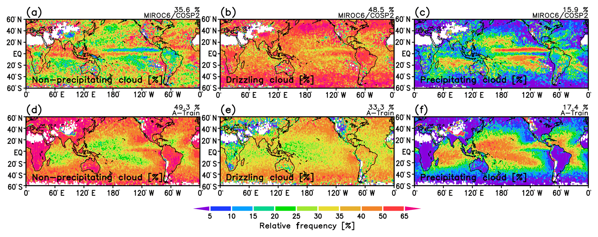
Figure 2Geographical maps of the fractional occurrence of (a, d) non-precipitating clouds ( dBZe), (b, e) drizzling clouds (−15 dBZe dBZe), and (c, f) precipitating clouds (0 dBZe <Zmax) obtained from (a–c) the MIROC6–COSP2 simulation of one full year and (d–f) the A-Train satellite observations for the period June 2006–April 2011. Global means of the occurrence frequency are shown at the top right of each panel.
3.1 Occurrence frequency of warm clouds
Figure 2 shows the geographical distributions of the fractional occurrences of SLWCs for non-precipitating, drizzling, and precipitating regimes obtained from the MIROC6 simulation and A-Train satellite observations. Note that although the reference A-Train statistics are shown at resolution, which is close to that of MIROC6–SPRINTARS, the statistics are constructed from the native CloudSat resolution (1.4×2.5 km) and subcolumns in the host model prepared by COSP (kilometer scale) to achieve a scale-aware model–satellite comparison.
We obtained 74.6 million SLWCs from the model and 7.8 million SLWCs from observations. The model generated more SLWCs than were present in the A-Train observations. This suggests that one full year of simulation with 3-hourly diagnosis is long enough, but note that this does not negate the possibility of the generation of SLWCs being too frequent in the model. In the A-Train satellite retrievals, many SLWCs are located over the typical stratocumulus (Sc) regions off the west coasts of California, Peru, Australia, Namibia, and the Canary Islands (not shown), where the non-precipitating regime is dominant (Fig. 2d). The MIROC6 finds 48.5 % drizzling regime versus 33.3 % in the A-Train retrievals (Figs. 2b and e). For the precipitating regime, although the global mean values of occurrence frequency are consistent with each other (15.9 % in MIROC6 and 17.4 % in A-Train), the geographical pattern is quite different, particularly over tropical oceans and continents (Figs. 2c and f), implying that the model has biases in the warm rain formation process (e.g., Jing et al., 2019) and/or the representation of cloud types (e.g., Huang et al., 2015).
These biases in MIROC6 can be interpreted in the context of the aerosol–cloud interactions parameterized in the model. In bulk microphysics models, the onset of rain is represented by the so-called autoconversion scheme, which is generally expressed as (e.g., Berry, 1968; Beheng, 1994; Khairoutdinov and Kogan, 2000)
where qc and qr are the liquid cloud water and rainwater mixing ratios, respectively; Nc is the cloud droplet number concentration; and Caut, α, and β are the prescribed (uncertain) constants. This formulation describes how the model forms rain in terms of uncertain parameters. Given that the CloudSat cloud profiling radar is sensitive to both cloud droplets and raindrops (Stephens and Haynes, 2007; Haynes et al., 2009), model–satellite comparisons (Fig. 2) offer useful evaluations of cloud-to-rain transition processes represented by Eq. (3), as also proposed by Kay et al. (2018).
3.2 Vertical microphysical structure
Figure 3 shows the CFODDs obtained from the MIROC6–COSP2 and A-Train observations, which are classified according to the MODIS-derived cloud-top effective radius (Re) in the 2.1 µm band as 5–12, 12–18, and 18–35 µm (Michibata et al., 2014). The radar reflectivity ranges (−30 to 20 dBZe) and the ICOD range (0 to 60) are divided linearly into 25 and 30 bins, respectively, following Suzuki et al. (2013).

Figure 3Contoured frequency by optical depth diagrams (CFODDs) obtained from (a–c) the MIROC6–COSP2 one full year simulation and (d–f) the A-Train satellite observations for the period June 2006–April 2011. CFODDs are classified according to the MODIS-derived cloud-top effective radius (Re) in the 2.1 µm band as (a, d) 5–12, (b, e) 12–18, and (c, f) 18–35 µm following Michibata et al. (2014).
Here, we demonstrate that CFODDs deduced from satellite observations illustrate systematic transitions from non-precipitating through drizzling to precipitating regimes as a function of Re and are consistent with previous observational findings showing the strong dependence of the onset of precipitation upon Re (Lebsock et al., 2008; Rosenfeld et al., 2012). On the other hand, MIROC6 simulates higher radar reflectivity even in the smallest Re category, revealing a bias in rain formation that is too early and too frequent (Suzuki et al., 2015). We attribute this discrepancy between the model and observations primarily to the following two factors: the bias in the updraft velocity (Nakajima et al., 2010; Takahashi et al., 2017a) at the subgrid scale and the uncertainty associated with the dependence of rain formation on aerosols (Wood, 2005; Suzuki et al., 2013) as characterized by β in Eq. (3). To evaluate this regime dependence of aerosol–cloud interactions (Sorooshian et al., 2009; Michibata et al., 2016; Chen et al., 2016, 2018), it is useful to investigate the differences in CFODDs from various environmental regimes (e.g., updraft and aerosol loading).
Thus, we defined 13 regions (Fig. 4) to examine the detailed aerosol–cloud interactions. This regional classification is based on previous warm rain studies with various research aims (e.g., Leon et al., 2008; Terai et al., 2015) and is summarized in Table 1. Statistics can also be examined separately over land and ocean (not shown) to investigate the differences in the CFODD transition in dynamic regimes (e.g., Takahashi et al., 2017b). Alternatively, users can define specific regions to suit their research purposes.
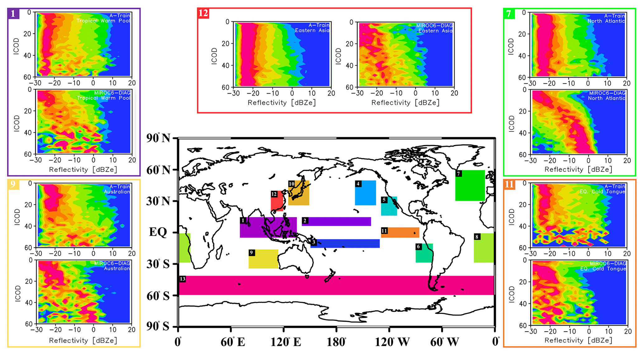
Figure 4Definition of the 13 regions used in the post-process package. An example of the regional CFODD analysis over the (red) Eastern Asian, (purple) Tropical Warm Pool, (yellow) Australian, (green) North Atlantic, and (orange) Equatorial Cold Tongue regions obtained from the MIROC6–COSP2 and the A-Train observations for the Re range µm. The color scale is the same as in Fig. 3.
Table 1Definition of the 13 regions used in the CFODD regional analysis, corresponding to the boxes in Fig. 4.
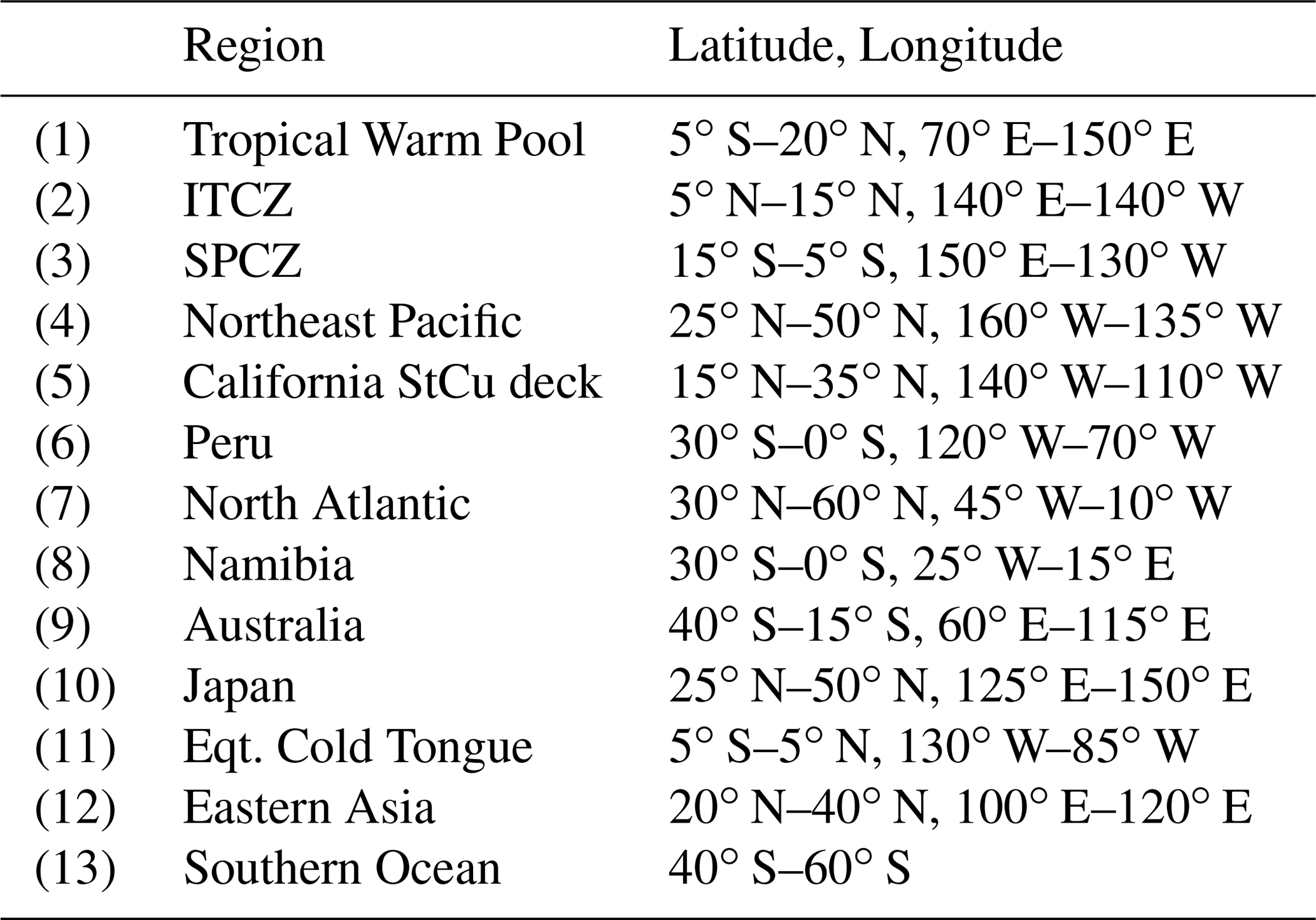
Figure 4 shows results from a regional CFODD analysis over five regions: Eastern Asia, Tropical Warm Pool, Equatorial Cold Tongue, North Atlantic, and Australia. CFODDs for the smallest Re range ( µm) are shown. This regional analysis reveals that the model does not always show a warm rain bias in all regions that is too early and/or too frequent. For example, the CFODDs over the Eastern Asian, Australian, and Equatorial Cold Tongue regions simulated by MIROC6 are in good agreement with those derived from the A-Train observations. The model accurately captures the non-precipitating regime in the smaller Re categories, suggesting that the model partially captures slower cloud-to-rain conversions in aerosol-abundant environments (Eastern Asia) and under calm stable conditions (Australia and Equatorial Cold Tongue). These results emphasize the importance of understanding the link between microphysics and dynamics (Chen et al., 2014; Zhang et al., 2016) if we wish to develop a more reliable representation of aerosol–cloud–precipitation interactions, but this is beyond the scope of this technical paper.
As discussed above, CFODDs provide valuable information on cloud-to-rain microphysical transitions associated with aerosol–cloud interactions and microphysics–dynamics interactions. Our new warm rain diagnostic tool will assist in process-oriented model evaluations with the synergistic use of A-Train multi-satellite observations.
This technical paper describes a new warm rain diagnostic tool implemented in the COSP2 satellite simulator package that extends its process-oriented diagnostic capabilities (Michibata et al., 2019b). We have introduced two new diagnostics: (1) the occurrence frequencies of non-precipitating clouds ( dBZe), drizzling clouds (−15 dBZe dBZe), and precipitating clouds (0 dBZe <Zmax) and 2) the PDF distributions of radar reflectivity profiles normalized by ICOD, the so-called contoured frequency by optical depth diagram (CFODD). These diagnostics make synergistic use of the CloudSat and MODIS simulators (Michibata et al., 2019c).
The diagnostic tool is controlled by the logical flags, “Lwr_occfreq” and “Lcfodd” in the namelist for COSP outputs. Users are now not required to output subcolumn parameters, such as the radar or lidar signals from the simulators of active sensors, which significantly increases the efficiency of model evaluation. Adding the inline warm rain diagnostics into COSP increases the computational cost only slightly (by around 0.8 %) when using the SX-ACE supercomputer system of the National Institute for Environmental Studies, Japan.
The inline warm rain diagnostic tool is intended to facilitate model evaluations that are efficient enough to be conducted within the model development loop, specifically by providing both “performance constraints” and “process-level fingerprints” (Fig. 1). The diagnostic tool has been designed to reveal potential uncertainties in modeled warm rain processes in GCMs more effectively and simply. The multi-platform products can also be extended to include other diagnostics for mixed-phase and ice clouds (e.g., Mülmenstädt et al., 2015; Kikuchi et al., 2017) in future work. Requests for specific diagnostics, particularly those requiring COSP subcolumn output for fast-process evaluations, are welcome.
The source code of COSP2 for the online diagnostics used in this study is available at https://doi.org/10.5281/zenodo.1442468 (Michibata et al., 2019b). Post-processing code and reference A-Train statistics can be found at https://doi.org/10.5281/zenodo.3370823 (Michibata et al., 2019c). The results of the MIROC6 simulation used to produce the figures are also included in the post-process package. The CloudSat data products can be obtained from the CloudSat Data Processing Center at CIRA/Colorado State University (http://www.cloudsat.cira.colostate.edu, last access: 8 October 2019).
TM and KS designed the research; TM implemented the new diagnostics into COSP2; TM, TO, and XJ tested the new tool on the MIROC6–COSP2 interface; KS reviewed and improved the code; TM analyzed the model and observational data; and TM and KS wrote the paper.
The authors declare that they have no conflict of interest.
We thank the developers of the COSP satellite simulator and the CFMIP community. This work has benefited from fruitful discussions with Alejandro Bodas-Salcedo, Robert Pincus, and Dustin Swales. The authors also thank Koji Ogochi for his testing and code optimization of COSP on MIROC6. Simulations by MIROC-SPRINTARS were executed on the SX-ACE supercomputer system of the National Institute for Environmental Studies, Japan. This study was supported by the following: the JSPS KAKENHI under grant numbers JP18J00301, JP19K14795, and JP19H05669; the Integrated Research Program for Advancing Climate Models (TOUGOU program) from the Ministry of Education, Culture, Sports, Science and Technology (MEXT), Japan; and the Collaborative Research Program of the Research Institute for Applied Mechanics, Kyushu University. Kentaroh Suzuki was supported by the NOAA Climate Program Office’s Modeling, Analysis, Predictions, and Projections program with grant number NA15OAR4310153. The authors are grateful to Johannes Mülmenstädt (Universität Leipzig) and two anonymous reviewers for providing constructive suggestions and comments that helped to improve the paper.
This research has been supported by the Japan Society for the Promotion of Science (grant nos. JP18J00301, JP19K14795, and JP19H05669), the Ministry of Education, Culture, Sports, Science and Technology (Integrated Research Program for Advancing Climate Models (TOUGOU program)), Kyushu University (Collaborative Research Program of the Research Institute for Applied Mechanics), and the NOAA Climate Program Office (grant no. NA15OAR4310153).
This paper was edited by Axel Lauer and reviewed by Johannes Mülmenstädt and two anonymous referees.
Bai, H., Gong, C., Wang, M., Zhang, Z., and L'Ecuyer, T.: Estimating precipitation susceptibility in warm marine clouds using multi-sensor aerosol and cloud products from A-Train satellites, Atmos. Chem. Phys., 18, 1763–1783, https://doi.org/10.5194/acp-18-1763-2018, 2018. a
Beheng, K. D.: A parameterization of warm cloud microphysical conversion processes, Atmos. Res., 33, 193–206, 1994. a
Berry, E. X.: Modification of the Warm Rain Process, in: Proc. First Conf. on Weather Modification, Albany, NY, Amer. Meteor. Soc, paper presented at 1st National Conf. on Weather Modification, 28 April–1 May, 81–85, 1968. a, b
Bodas-Salcedo, A., Webb, M. J., Bony, S., Chepfer, H., Dufresne, J.-L., Klein, S. A., Zhang, Y., Marchand, R., Haynes, J. M., Pincus, R., and John, V. O.: COSP: Satellite simulation software for model assessment, B. Am. Meteorol. Soc., 92, 1023–1043, https://doi.org/10.1175/2011BAMS2856.1, 2011. a, b
Boucher, O., Randall, D., Artaxo, P., Bretherton, C., Feingold, G., Forster, P., Kerminen, V.-M., Kondo, Y., Liao, H., Lohmann, U., Rasch, P., Satheesh, S. K., Sherwood, S., Stevens, B., and Zhang, X. Y.: Clouds and aerosols, Cambridge University Press, Cambridge, UK, 571–657, https://doi.org/10.1017/CBO9781107415324.016, 2013. a
Brenguier, J.-L., Pawlowska, H., Schüller, L., Preusker, R., Fischer, J., and Fouquart, Y.: Radiative Properties of Boundary Layer Clouds: Droplet Effective Radius versus Number Concentration, J. Atmos. Sci., 57, 803–821, https://doi.org/10.1175/1520-0469(2000)057<0803:RPOBLC>2.0.CO;2, 2000. a
Bretherton, C. S.: Insights into low-latitude cloud feedbacks from high-resolution models, Philos. T. Roy. Soc. A, 373, 20140415, https://doi.org/10.1098/rsta.2014.0415, 2015. a
Cesana, G. and Chepfer, H.: How well do climate models simulate cloud vertical structure? A comparison between CALIPSO-GOCCP satellite observations and CMIP5 models, Geophys. Res. Lett., 39, 1–6, https://doi.org/10.1029/2012GL053153, 2012. a
Chen, J., Liu, Y., Zhang, M., and Peng, Y.: New understanding and quantification of the regime dependence of aerosol-cloud interaction for studying aerosol indirect effects, Geophys. Res. Lett., 43, 1780–1787, https://doi.org/10.1002/2016GL067683, 2016. a
Chen, J., Liu, Y., Zhang, M., and Peng, Y.: Height Dependency of Aerosol-Cloud Interaction Regimes, J. Geophys. Res.-Atmos., 123, 491–506, https://doi.org/10.1002/2017JD027431, 2018. a
Chen, Y.-C., Christensen, M. W., Stephens, G. L., and Seinfeld, J. H.: Satellite-based estimate of global aerosol-cloud radiative forcing by marine warm clouds, Nat. Geosci., 7, 643–646, https://doi.org/10.1038/ngeo2214, 2014. a
Chepfer, H., Bony, S., Winker, D., Chiriaco, M., Dufresne, J. L., and Sèze, G.: Use of CALIPSO lidar observations to evaluate the cloudiness simulated by a climate model, Geophys. Res. Lett., 35, L15704, https://doi.org/10.1029/2008GL034207, 2008. a
Chikira, M. and Sugiyama, M.: A cumulus parameterization with state-dependent entrainment rate. Part I: Description and sensitivity to temperature and humidity profiles, J. Atmos. Sci., 67, 2171–2193, https://doi.org/10.1175/2010JAS3316.1, 2010. a
Christensen, M. W., Chen, Y. C., and Stephens, G. L.: Aerosol indirect effect dictated by liquid clouds, J. Geophys. Res., 121, 14636–14650, https://doi.org/10.1002/2016JD025245, 2016. a
Eyring, V., Bony, S., Meehl, G. A., Senior, C. A., Stevens, B., Stouffer, R. J., and Taylor, K. E.: Overview of the Coupled Model Intercomparison Project Phase 6 (CMIP6) experimental design and organization, Geosci. Model Dev., 9, 1937–1958, https://doi.org/10.5194/gmd-9-1937-2016, 2016. a
Gettelman, A. and Sherwood, S. C.: Processes Responsible for Cloud Feedback, Current Climate Change Reports, 179–189, https://doi.org/10.1007/s40641-016-0052-8, 2016. a
Gryspeerdt, E. and Stier, P.: Regime-based analysis of aerosol-cloud interactions, Geophys. Res. Lett., 39, L21802, https://doi.org/10.1029/2012GL053221, 2012. a
Haynes, J. M., Marchand, R. T., Luo, Z., Bodas-Salcedo, A., and Stephens, G. L.: A multipurpose radar simulation package: QuickBeam, B. Am. Meteorol. Soc., 88, 1723–1727, https://doi.org/10.1175/BAMS-88-11-1723, 2007. a
Haynes, J. M., L'Ecuyer, T. S., Stephens, G. L., Miller, S. D., Mitrescu, C., Wood, N. B., and Tanelli, S.: Rainfall retrieval over the ocean with spaceborne W-band radar, J. Geophys. Res.-Atmos., 114, D00A22, https://doi.org/10.1029/2008JD009973, 2009. a, b
Huang, L., Jiang, J. H., Wang, Z., Su, H., Deng, M., and Massie, S.: Climatology of cloud water content associated with different cloud types observed by A-Train satellites, J. Geophys. Res.-Atmos., 120, 4196–4212, https://doi.org/10.1002/2014JD022779, 2015. a
Jing, X., Suzuki, K., Guo, H., Goto, D., Ogura, T., Koshiro, T., and Mülmenstädt, J.: A Multimodel Study on Warm Precipitation Biases in Global Models Compared to Satellite Observations, J. Geophys. Res.-Atmos., 122, 11806–11824, https://doi.org/10.1002/2017JD027310, 2017. a
Jing, X., Suzuki, K., and Michibata, T.: The Key Role of Warm Rain Parameterization in Determining the Aerosol Indirect Effect in a Global Climate Model, J. Climate, 32, 4409–4430, https://doi.org/10.1175/jcli-d-18-0789.1, 2019. a
Kay, J. E., L'Ecuyer, T., Pendergrass, A., Chepfer, H., Guzman, R., and Yettella, V.: Scale-Aware and Definition-Aware Evaluation of Modeled Near-Surface Precipitation Frequency Using CloudSat Observations, J. Geophys. Res.-Atmos., 123, 4294–4309, https://doi.org/10.1002/2017JD028213, 2018. a, b, c, d, e
Khairoutdinov, M. and Kogan, Y.: A new cloud physics parameterization in a large-eddy simulation model of marine stratocumulus, Mon. Weather Rev., 128, 229–243, 2000. a
Kikuchi, M., Okamoto, H., Sato, K., Suzuki, K., Cesana, G., Hagihara, Y., Takahashi, N., Hayasaka, T., and Oki, R.: Development of Algorithm for Discriminating Hydrometeor Particle Types with a Synergistic Use of CloudSat and CALIPSO, J. Geophys. Res.-Atmos., 122, 11022–11044, https://doi.org/10.1002/2017JD027113, 2017. a
Klein, S. A. and Jakob, C.: Validation and sensitivities of frontal clouds simulated by the ECMWF model, Mon. Weather Rev., 127, 2514–2531, https://doi.org/10.1175/1520-0493(1999)127<2514:vasofc>2.0.co;2, 1999. a
Konsta, D., Dufresne, J. L., Chepfer, H., Idelkadi, A., and Cesana, G.: Use of A-train satellite observations (CALIPSO–PARASOL) to evaluate tropical cloud properties in the LMDZ5 GCM, Clim. Dynam., 47, 1263–1284, https://doi.org/10.1007/s00382-015-2900-y, 2016. a, b
Kubar, T. L., Hartmann, D. L., and Wood, R.: Understanding the Importance of Microphysics and Macrophysics for Warm Rain in Marine Low Clouds. Part I: Satellite Observations, J. Atmos. Sci., 66, 2953–2972, https://doi.org/10.1175/2009JAS3071.1, 2009. a
Lebsock, M. D., Stephens, G. L., and Kummerow, C.: Multisensor satellite observations of aerosol effects on warm clouds, J. Geophys. Res., 113, D15205, https://doi.org/10.1029/2008JD009876, 2008. a
L'Ecuyer, T. S. and Jiang, J. H.: Touring the atmosphere aboard the A-Train, Phys. Today, 63, 36–41, https://doi.org/10.1063/1.3653856, 2010. a
L'Ecuyer, T. S., Beaudoing, H. K., Rodell, M., Olson, W., Lin, B., Kato, S., Clayson, C. A., Wood, E., Sheffield, J., Adler, R., Huffman, G., Bosilovich, M., Gu, G., Robertson, F., Houser, P. R., Chambers, D., Famiglietti, J. S., Fetzer, E., Liu, W. T., Gao, X., Schlosser, C. A., Clark, E., Lettenmaier, D. P., and Hilburn, K.: The observed state of the energy budget in the early 21st century, J. Climate, 28, 8319–8346, https://doi.org/10.1175/JCLI-D-14-00556.1, 2015. a
Leon, D. C., Wang, Z., and Liu, D.: Climatology of drizzle in marine boundary layer clouds based on 1 year of data from CloudSat and Cloud-Aerosol Lidar and Infrared Pathfinder Satellite Observations (CALIPSO), J. Geophys. Res., 113, D00A14, https://doi.org/10.1029/2008JD009835, 2008. a
Ma, P. L., Rasch, P. J., Chepfer, H., Winker, D. M., and Ghan, S. J.: Observational constraint on cloud susceptibility weakened by aerosol retrieval limitations, Nat. Commun., 9, 2640, https://doi.org/10.1038/s41467-018-05028-4, 2018. a
Mace, G. G., Marchand, R., Zhang, Q., and Stephens, G.: Global hydrometeor occurrence as observed by CloudSat: Initial observations from summer 2006, Geophys. Res. Lett., 34, L09808, https://doi.org/10.1029/2006GL029017, 2007. a
Maloney, E. D., Gettelman, A., Ming, Y., Neelin, J. D., Barrie, D., Mariotti, A., Chen, C.-C., Coleman, D. R. B., Kuo, Y.-H., Singh, B., Annamalai, H., Berg, A., Booth, J. F., Camargo, S. J., Dai, A., Gonzalez, A., Hafner, J., Jiang, X., Jing, X., Kim, D., Kumar, A., Moon, Y., Naud, C. M., Sobel, A. H., Suzuki, K., Wang, F., Wang, J., Wing, A. A., Xu, X., and Zhao, M.: Process-Oriented Evaluation of Climate and Weather Forecasting Models, B. Am. Meteorol. Soc., 100, 1665–1686, https://doi.org/10.1175/bams-d-18-0042.1, 2019. a
Marchand, R. and Ackerman, T.: An analysis of cloud cover in multiscale modeling framework global climate model simulations using 4 and 1 km horizontal grids, J. Geophys. Res.-Atmos., 115, D16207, https://doi.org/10.1029/2009JD013423, 2010. a
Marchand, R., Mace, G. G., Ackerman, T., and Stephens, G.: Hydrometeor detection using CloudSat – An Earth-orbiting 94-GHz cloud radar, J. Atmos. Ocean. Tech., 25, 519–533, https://doi.org/10.1175/2007JTECHA1006.1, 2008. a
Marchand, R., Haynes, J., Mace, G. G., Ackerman, T., and Stephens, G.: A comparison of simulated cloud radar output from the multiscale modeling framework global climate model with CloudSat cloud radar observations, J. Geophys. Res., 114, D00A20, https://doi.org/10.1029/2008JD009790, 2009. a
Masunaga, H., Matsui, T., Tao, W.-K., Hou, A. Y., Kummerow, C. D., Nakajima, T., Bauer, P., Olson, W. S., Sekiguchi, M., and Nakajima, T. Y.: Satellite Data Simulator Unit A multisensor, multispectral Satellite Simulator Package, B. Am. Meteorol. Soc., 91, 1625–1632, https://doi.org/10.1175/2010BAMS2809.1, 2010. a
Matus, A. V. and L'Ecuyer, T. S.: The role of cloud phase in Earth's radiation budget, J. Geophys. Res.-Atmos., 122, 1–20, https://doi.org/10.1002/2016JD025951, 2017. a
Medeiros, B. and Stevens, B.: Revealing differences in GCM representations of low clouds, Clim. Dynam., 36, 385–399, https://doi.org/10.1007/s00382-009-0694-5, 2011. a
Michibata, T. and Takemura, T.: Evaluation of autoconversion schemes in a single model framework with satellite observations, J. Geophys. Res., 120, 9570–9590, https://doi.org/10.1002/2015JD023818, 2015. a
Michibata, T., Kawamoto, K., and Takemura, T.: The effects of aerosols on water cloud microphysics and macrophysics based on satellite-retrieved data over East Asia and the North Pacific, Atmos. Chem. Phys., 14, 11935–11948, https://doi.org/10.5194/acp-14-11935-2014, 2014. a, b, c
Michibata, T., Suzuki, K., Sato, Y., and Takemura, T.: The source of discrepancies in aerosol–cloud–precipitation interactions between GCM and A-Train retrievals, Atmos. Chem. Phys., 16, 15413–15424, https://doi.org/10.5194/acp-16-15413-2016, 2016. a, b, c, d
Michibata, T., Suzuki, K., Sekiguchi, M., and Takemura, T.: Prognostic precipitation in the MIROC6-SPRINTARS GCM: Description and evaluation against satellite observations, J. Adv. Model. Earth Sy., 11, 839–860, https://doi.org/10.1029/2018MS001596, 2019a. a
Michibata, T., Suzuki, K., Ogura, T., and Jing, X.: Scripts for the publication “Incorporation of inline warm rain diagnostics into the COSP2 satellite simulator for process-oriented model evaluation” (Version 1.0.0), Zenodo, https://doi.org/10.5281/zenodo.1442468, 2019b. a, b
Michibata, T., Suzuki, K., Ogura, T., and Jing, X.: Data for the publication “Incorporation of inline warm rain diagnostics into the COSP2 satellite simulator for process-oriented model evaluation” (Version 1.0.0), Zenodo, https://doi.org/10.5281/zenodo.3370823, 2019c. a, b
Mülmenstädt, J. and Feingold, G.: The Radiative Forcing of Aerosol–Cloud Interactions in Liquid Clouds: Wrestling and Embracing Uncertainty, Current Climate Change Reports, 4, 23–40, https://doi.org/10.1007/s40641-018-0089-y, 2018. a
Mülmenstädt, J., Sourdeval, O., Delanoë, J., and Quaas, J.: Frequency of occurrence of rain from liquid-, mixed-, and ice-phase clouds derived from A-Train satellite retrievals, Geophys. Res. Lett., 42, 6502–6509, https://doi.org/10.1002/2015GL064604, 2015. a
Myhre, G., Shindell, D., Bréon, F.-M., Collins, W., Fuglestvedt, J., Huang, J., Koch, D., Lamarque, J.-F., Lee, D., Mendoza, B., Nakajima, T., Robock, A., Stephens, G., Takemura, T., and Zhang, H.: Anthropogenic and natural radiative forcing, Cambridge University Press, Cambridge, UK, 659–740, https://doi.org/10.1017/CBO9781107415324.018, 2013. a
Nakajima, T. Y., Suzuki, K., and Stephens, G. L.: Droplet Growth in Warm Water Clouds Observed by the A-Train. Part II: A Multisensor View, J. Atmos. Sci., 67, 1897–1907, https://doi.org/10.1175/2010JAS3276.1, 2010. a, b
Nam, C. C. W., Johannes Quaas, Neggers, R., Drian, C. S.-L., and Isotta, F.: Evaluation of boundary layer cloud parameterizations in the ECHAM5 general circulationmodel using CALIPSO and CloudSat satellite data, J. Adv. Model. Earth Sy., 6, 300–314, https://doi.org/10.1002/2013MS000277, 2014. a
Park, S. and Bretherton, C. S.: The University of Washington shallow convection and moist turbulence schemes and their impact on climate simulations with the community atmosphere model, J. Climate, 22, 3449–3469, https://doi.org/10.1175/2008JCLI2557.1, 2009. a
Partain, P.: Cloudsat ECMWF-AUX auxiliary data process description and interface control document, Cooperative Institute for Research in the Atmosphere, Colorado State University, p. 10, 2007. a
Patel, P. N., Gautam, R., Michibata, T., and Gadhavi, H.: Strengthened Indian summer monsoon precipitation susceptibility linked to dust‐induced ice cloud modification, Geophys. Res. Lett., 46, 8431–8441, https://doi.org/10.1029/2018GL081634, 2019. a
Pincus, R., Platnick, S., Ackerman, S. A., Hemler, R. S., and Patrick Hofmann, R. J.: Reconciling simulated and observed views of clouds: MODIS, ISCCP, and the limits of instrument simulators, J. Climate, 25, 4699–4720, https://doi.org/10.1175/JCLI-D-11-00267.1, 2012. a
Polonsky, I. N.: Level 2 cloud optical depth product process description and interface control document, Cooperative Institute for Research in the Atmosphere, Colorado State University, p. 21, 2008. a
Quaas, J.: Approaches to Observe Anthropogenic Aerosol-Cloud Interactions, Current Climate Change Reports, 1, 297–304, https://doi.org/10.1007/s40641-015-0028-0, 2015. a
Rosenfeld, D., Wang, H., and Rasch, P. J.: The roles of cloud drop effective radius and LWP in determining rain properties in marine stratocumulus, Geophys. Res. Lett., 39, L13801, https://doi.org/10.1029/2012GL052028, 2012. a
Rosenfeld, D., Zhu, Y., Minghuai, W., Zheng, Y., Goren, T., and Yu, S.: Aerosol-driven droplet concentrations dominate converage and water of oceanic low level clouds, Science, 363, AAV0566, https://doi.org/10.1126/SCIENCE.AAV0566, 2019. a
Smalley, M., L'Ecuyer, T., Lebsock, M., and Haynes, J.: A Comparison of Precipitation Occurrence from the NCEP Stage IV QPE Product and the CloudSat Cloud Profiling Radar, J. Hydrometeorol., 15, 444–458, https://doi.org/10.1175/JHM-D-13-048.1, 2014. a
Sorooshian, A., Feingold, G., Lebsock, M. D., Jiang, H., and Stephens, G. L.: On the precipitation susceptibility of clouds to aerosol perturbations, Geophys. Res. Lett., 36, L13803, https://doi.org/10.1029/2009GL038993, 2009. a
Sorooshian, A., Wang, Z., Feingold, G., and L'Ecuyer, T. S.: A satellite perspective on cloud water to rain water conversion rates and relationships with environmental conditions, J. Geophys. Res.-Atmos., 118, 6643–6650, https://doi.org/10.1002/jgrd.50523, 2013. a
Stephens, G., Winker, D., Pelon, J., Trepte, C., Vane, D., Yuhas, C., L'Ecuyer, T., and Lebsock, M.: CloudSat and CALIPSO within the A-Train: Ten years of actively observing the Earth system, B. Am. Meteorol. Soc., 99, 569–581, https://doi.org/10.1175/BAMS-D-16-0324.1, 2018. a
Stephens, G. L. and Haynes, J. M.: Near global observations of the warm rain coalescence process, Geophys. Res. Lett., 34, L20805, https://doi.org/10.1029/2007GL030259, 2007. a
Stephens, G. L., Vane, D. G., Boain, R. J., Mace, G. G., Sassen, K., Wang, Z., Illingworth, A. J., O'Connor, E. J., Rossow, W. B., Durden, S. L., Miller, S. D., Austin, R. T., Benedetti, A., Mitrescu, C., and Team, T. C. S.: The Cloudsat mission and the A-Train, B. Am. Meteorol. Soc., 83, 1771–1790, https://doi.org/10.1175/BAMS-83-12-1771, 2002. a
Stephens, G. L., Vane, D. G., Tanelli, S., Im, E., Durden, S., Rokey, M., Reinke, D., Partain, P., Mace, G. G., Austin, R., L'Ecuyer, T., Haynes, J., Lebsock, M., Suzuki, K., Waliser, D., Wu, D., Kay, J., Gettelman, A., Wang, Z., and Marchand, R.: CloudSat mission: Performance and early science after the first year of operation, J. Geophys. Res.-Atmos., 113, D00A18, https://doi.org/10.1029/2008JD009982, 2008. a
Suzuki, K., Nakajima, T. Y., and Stephens, G. L.: Particle Growth and Drop Collection Efficiency of Warm Clouds as Inferred from Joint CloudSat and MODIS Observations, J. Atmos. Sci., 67, 3019–3032, https://doi.org/10.1175/2010JAS3463.1, 2010. a, b
Suzuki, K., Stephens, G. L., van den Heever, S. C., and Nakajima, T. Y.: Diagnosis of the Warm Rain Process in Cloud-Resolving Models Using Joint CloudSat and MODIS Observations, J. Atmos. Sci., 68, 2655–2670, https://doi.org/10.1175/JAS-D-10-05026.1, 2011. a
Suzuki, K., Stephens, G. L., and Lebsock, M. D.: Aerosol effect on the warm rain formation process: Satellite observations and modeling, J. Geophys. Res., 118, 170–184, https://doi.org/10.1002/jgrd.50043, 2013. a, b, c
Suzuki, K., Stephens, G., Bodas-Salcedo, A., Wang, M., Golaz, J.-C., Yokohata, T., and Koshiro, T.: Evaluation of the Warm Rain Formation Process in Global Models with Satellite Observations, J. Atmos. Sci., 72, 3996–4014, https://doi.org/10.1175/JAS-D-14-0265.1, 2015. a, b
Swales, D. J., Pincus, R., and Bodas-Salcedo, A.: The Cloud Feedback Model Intercomparison Project Observational Simulator Package: Version 2, Geosci. Model Dev., 11, 77–81, https://doi.org/10.5194/gmd-11-77-2018, 2018. a, b, c, d
Szczodrak, M., Austin, P. H., and Krummel, P. B.: Variability of Optical Depth and Effective Radius in Marine Stratocumulus Clouds, J. Atmos. Sci., 58, 2912–2926, https://doi.org/10.1175/1520-0469(2001)058<2912:VOODAE>2.0.CO;2, 2001. a
Takahashi, H., Lebsock, M., Suzuki, K., Stephens, G., and Wang, M.: An investigation of microphysics and subgrid-scale variability in warm-rain clouds using the A-Train observations and a multiscale modeling framework, J. Geophys. Res.-Atmos., 122, 7493–7504, https://doi.org/10.1002/2016JD026404, 2017a. a
Takahashi, H., Suzuki, K., and Stephens, G.: Land–ocean differences in the warm-rain formation process in satellite and ground-based observations and model simulations, Q. J. Roy. Meteorol. Soc., 143, 1804–1815, https://doi.org/10.1002/qj.3042, 2017b. a
Tatebe, H., Ogura, T., Nitta, T., Komuro, Y., Ogochi, K., Takemura, T., Sudo, K., Sekiguchi, M., Abe, M., Saito, F., Chikira, M., Watanabe, S., Mori, M., Hirota, N., Kawatani, Y., Mochizuki, T., Yoshimura, K., Takata, K., O'ishi, R., Yamazaki, D., Suzuki, T., Kurogi, M., Kataoka, T., Watanabe, M., and Kimoto, M.: Description and basic evaluation of simulated mean state, internal variability, and climate sensitivity in MIROC6, Geosci. Model Dev., 12, 2727–2765, https://doi.org/10.5194/gmd-12-2727-2019, 2019. a
Terai, C. R., Wood, R., and Kubar, T. L.: Satellite estimates of precipitation susceptibility in low-level marine stratiform clouds, J. Geophys. Res., 120, 8878–8889, https://doi.org/10.1002/2015JD023319, 2015. a
Thayer-Calder, K., Gettelman, A., Craig, C., Goldhaber, S., Bogenschutz, P. A., Chen, C.-C., Morrison, H., Höft, J., Raut, E., Griffin, B. M., Weber, J. K., Larson, V. E., Wyant, M. C., Wang, M., Guo, Z., and Ghan, S. J.: A unified parameterization of clouds and turbulence using CLUBB and subcolumns in the Community Atmosphere Model, Geosci. Model Dev., 8, 3801–3821, https://doi.org/10.5194/gmd-8-3801-2015, 2015. a
Tsushima, Y., Brient, F., Klein, S. A., Konsta, D., Nam, C. C., Qu, X., Williams, K. D., Sherwood, S. C., Suzuki, K., and Zelinka, M. D.: The Cloud Feedback Model Intercomparison Project (CFMIP) Diagnostic Codes Catalogue – metrics, diagnostics and methodologies to evaluate, understand and improve the representation of clouds and cloud feedbacks in climate models, Geosci. Model Dev., 10, 4285–4305, https://doi.org/10.5194/gmd-10-4285-2017, 2017. a, b
Turner, S., Brenguier, J.-L., and Lac, C.: A subgrid parameterization scheme for precipitation, Geosci. Model Dev., 5, 499–521, https://doi.org/10.5194/gmd-5-499-2012, 2012. a
Wang, M., Ghan, S., Liu, X., L'Ecuyer, T. S., Zhang, K., Morrison, H., Ovchinnikov, M., Easter, R., Marchand, R., Chand, D., Qian, Y., and Penner, J. E.: Constraining cloud lifetime effects of aerosols using A-Train satellite observations, Geophys. Res. Lett., 39, L15709, https://doi.org/10.1029/2012GL052204, 2012. a
Watanabe, M., Emori, S., Satoh, M., and Miura, H.: A PDF-based hybrid prognostic cloud scheme for general circulation models, Clim. Dynam., 33, 795–816, https://doi.org/10.1007/s00382-008-0489-0, 2009. a
Webb, M., Senior, C., Bony, S., and Morcrette, J.-J.: Combining ERBE and ISCCP data to assess clouds in the Hadley Centre, ECMWF and LMD atmospheric climate models, Clim. Dynam., 17, 905–922, https://doi.org/10.1007/s003820100157, 2001. a
Webb, M. J., Andrews, T., Bodas-Salcedo, A., Bony, S., Bretherton, C. S., Chadwick, R., Chepfer, H., Douville, H., Good, P., Kay, J. E., Klein, S. A., Marchand, R., Medeiros, B., Siebesma, A. P., Skinner, C. B., Stevens, B., Tselioudis, G., Tsushima, Y., and Watanabe, M.: The Cloud Feedback Model Intercomparison Project (CFMIP) contribution to CMIP6, Geosci. Model Dev., 10, 359–384, https://doi.org/10.5194/gmd-10-359-2017, 2017. a, b
Wood, R.: Drizzle in stratiform boundary layer clouds. Part II: Microphysical aspects., J. Atmos. Sci., 62, 3034–3050, 2005. a
Wood, R., Kubar, T. L., and Hartmann, D. L.: Understanding the importance of microphysics and macrophysics for warm rain in marine low clouds. Part II: Heuristic models of rain formation, J. Atmos. Sci., 66, 2973–2990, https://doi.org/10.1175/2009JAS3072.1, 2009. a
Zhang, S., Wang, M., Ghan, S. J., Ding, A., Wang, H., Zhang, K., Neubauer, D., Lohmann, U., Ferrachat, S., Takeamura, T., Gettelman, A., Morrison, H., Lee, Y., Shindell, D. T., Partridge, D. G., Stier, P., Kipling, Z., and Fu, C.: On the characteristics of aerosol indirect effect based on dynamic regimes in global climate models, Atmos. Chem. Phys., 16, 2765–2783, https://doi.org/10.5194/acp-16-2765-2016, 2016. a