SKRIPS v1.0: a regional coupled ocean–atmosphere modeling framework (MITgcm–WRF) using ESMF/NUOPC, description and preliminary results for the Red Sea

A new regional coupled ocean–atmosphere model is developed and its implementation is presented in this paper. The coupled model is based on two open-source community model components: the MITgcm ocean model and the Weather Research and Forecasting (WRF) atmosphere model. The coupling between these components is performed using ESMF (Earth System Modeling Framework) and implemented according to National United Operational Prediction Capability (NUOPC) protocols. The coupled model is named the Scripps–KAUST Regional Integrated Prediction System (SKRIPS). SKRIPS is demonstrated with a real-world example by simulating a 30 d period including a series of extreme heat events occurring on the eastern shore of the Red Sea region in June 2012. The results obtained by using the coupled model, along with those in forced stand-alone oceanic or atmospheric simulations, are compared with observational data and reanalysis products. We show that the coupled model is capable of performing coupled ocean–atmosphere simulations, although all configurations of coupled and uncoupled models have good skill in modeling the heat events. In addition, a scalability test is performed to investigate the parallelization of the coupled model. The results indicate that the coupled model code scales well and the ESMF/NUOPC coupler accounts for less than 5 % of the total computational resources in the Red Sea test case. The coupled model and documentation are available at https://library.ucsd.edu/dc/collection/bb1847661c (last access: 26 September 2019), and the source code is maintained at https://github.com/iurnus/scripps_kaust_model (last access: 26 September 2019).

1 Introduction

Accurate and efficient forecasting of oceanic and atmospheric circulation is essential for a wide variety of high-impact societal needs, including extreme weather and climate events (Kharin and Zwiers, 2000; Chen et al., 2007), environmental protection and coastal management (Warner et al., 2010), management of fisheries (Roessig et al., 2004), marine conservation (Harley et al., 2006), water resources (Fowler and Ekström, 2009), and renewable energy (Barbariol et al., 2013). Effective forecasting relies on high model fidelity and accurate initialization of the models with the observed state of the coupled ocean–atmosphere system. Although global coupled models are now being implemented with increased resolution, higher-resolution regional coupled models, if properly driven by the boundary conditions, can provide an affordable way to study air–sea feedback for frontal-scale processes.

A number of regional coupled ocean–atmosphere models have been developed for various goals in the past decades. An early example of building a regional coupled model for realistic simulations focused on accurate weather forecasting in the Baltic Sea (Gustafsson et al., 1998; Hagedorn et al., 2000; Doscher et al., 2002) and showed that the coupled model improved the SST (sea surface temperature) and atmospheric circulation forecast. Enhanced numerical stability in the coupled simulation was also observed. These early attempts were followed by other practitioners in ocean-basin-scale climate simulations (e.g., Huang et al., 2004; Aldrian et al., 2005; Xie et al., 2007; Seo et al., 2007; Somot et al., 2008; Fang et al., 2010; Boé et al., 2011; Zou and Zhou, 2012; Gualdi et al., 2013; Van Pham et al., 2014; Chen and Curcic, 2016; Seo, 2017). For example, Huang et al. (2004) implemented a regional coupled model to study three major important patterns contributing to the variability and predictability of the Atlantic climate. The study suggested that these patterns originate from air–sea coupling within the Atlantic Ocean or by the oceanic response to atmospheric intrinsic variability. Seo et al. (2007) studied the nature of ocean–atmosphere feedbacks in the presence of oceanic mesoscale eddy fields in the eastern Pacific Ocean sector. The evolving SST fronts were shown to drive an unambiguous response of the atmospheric boundary layer in the coupled model and lead to model anomalies of wind stress curl, wind stress divergence, surface heat flux, and precipitation that resemble observations. This study helped substantiate the importance of ocean–atmosphere feedbacks involving oceanic mesoscale variability features.

In addition to basin-scale climate simulations, regional coupled models are also used to study weather extremes. For example, the COAMPS (Coupled Ocean/Atmosphere Mesoscale Prediction System) was applied to investigate idealized tropical cyclone events (Hodur, 1997). This work was then followed by other realistic extreme weather studies. Another example is the investigation of extreme bora wind events in the Adriatic Sea using different regional coupled models (Loglisci et al., 2004; Pullen et al., 2006; Ricchi et al., 2016). The coupled simulation results demonstrated improvements in describing the air–sea interaction processes by taking into account oceanic surface heat fluxes and wind-driven ocean surface wave effects (Loglisci et al., 2004; Ricchi et al., 2016). It was also found in model simulations that SST after bora wind events had a stabilizing effect on the atmosphere, reducing the atmospheric boundary layer mixing and yielding stronger near-surface wind (Pullen et al., 2006). Regional coupled models were also used for studying the forecasts of hurricanes, including hurricane path, hurricane intensity, SST variation, and wind speed (Bender and Ginis, 2000; Chen et al., 2007; Warner et al., 2010).

Regional coupled modeling systems also play important roles in studying the effect of surface variables (e.g., surface evaporation, precipitation, surface roughness) in the coupling processes of oceans or lakes. One example is the study conducted by Powers and Stoelinga (2000), who developed a coupled model and investigated the passage of atmospheric fronts over the Lake Erie region. Sensitivity analysis was performed to demonstrate that parameterization of lake surface roughness in the atmosphere model can improve the calculation of wind stress and heat flux. Another example is the investigation of Caspian Sea levels by Turuncoglu et al. (2013), who compared a regional coupled model with uncoupled models and demonstrated the improvement of the coupled model in capturing the response of Caspian Sea levels to climate variability.

In the past 10 years, many regional coupled models have been developed using modern model toolkits (Zou and Zhou, 2012; Turuncoglu et al., 2013; Turuncoglu, 2019) and include waves (Warner et al., 2010; Chen and Curcic, 2016), sediment transport (Warner et al., 2010), sea ice (Van Pham et al., 2014), and chemistry packages (He et al., 2015). However, this work was motivated by the need for a coupled regional ocean–atmosphere model implemented using an efficient coupling framework and with compatible state estimation capabilities in both ocean and atmosphere. The goal of this work is to (1) introduce the design of the newly developed regional coupled ocean–atmosphere modeling system, (2) describe the implementation of the modern coupling framework, (3) validate the coupled model using a real-world example, and (4) demonstrate and discuss the parallelization of the coupled model. In the coupled system, the oceanic model component is the MIT general circulation model (MITgcm) (Marshall et al., 1997) and the atmospheric model component is the Weather Research and Forecasting (WRF) model (Skamarock et al., 2019). To couple the model components in the present work, the Earth System Modeling Framework (ESMF) (Hill et al., 2004) is used because of its advantages in conservative re-gridding capability, calendar management, logging and error handling, and parallel communications. The National United Operational Prediction Capability (NUOPC) layer in ESMF (Sitz et al., 2017) is also used between model components and ESMF. Using the NUOPC layer can simplify the implementation of component synchronization, execution, and other common tasks in the coupling. The innovations in our work are (1) we use ESMF/NUOPC, which is a community-supported computationally efficient coupling software for earth system models, and (2) we use MITgcm together with WRF, both of which work with the Data Assimilation Research Testbed (DART) (Anderson and Collins, 2007; Hoteit et al., 2013). The resulting coupled model is being developed for coupled data assimilation and subseasonal to seasonal (S2S) forecasting. By coupling WRF and MITgcm for the first time with ESMF, we can provide an alternative regional coupled model resource to a wider community of users. These atmospheric and oceanic model components have an active and well-supported user base.

After implementing the new coupled model, we demonstrate it on a series of heat events that occurred on the eastern shore of the Red Sea region in June 2012. The simulated surface variables of the Red Sea (e.g., sea surface temperature, 2 m temperature, and surface heat fluxes) are examined and validated against available observational data and reanalysis products. To demonstrate that the coupled model can perform coupled ocean–atmosphere simulations, the results are compared with those obtained using stand-alone oceanic or atmospheric models. This paper focuses on the technical aspects of SKRIPS and is not a full investigation of the importance of coupling for these extreme events. In addition, a scalability test of the coupled model is performed to investigate its parallel capability.

The rest of this paper is organized as follows. The description of the individual modeling components and the design of the coupled modeling system are detailed in Sect. 2. Section 3 introduces the design of the validation experiment and the validation data. Section 4 discusses the preliminary results in the validation test. Section 5 details the parallelization test of the coupled model. The last section concludes the paper and presents an outlook for future work.

2 Model description

The newly developed regional coupled modeling system is introduced in this section. The general design of the coupled model, descriptions of individual components, and ESMF/NUOPC coupling framework are presented below.

2.1 General design

The schematic description of the coupled model is shown in Fig. 1. The coupled model is comprised of five components: the oceanic component MITgcm, the atmospheric component WRF, the MITgcm–ESMF and WRF–ESMF interfaces, and the ESMF coupler. They are to be detailed in the following sections.

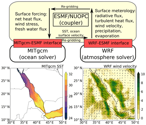
Figure 1 The schematic description of the coupled ocean–atmosphere model. The yellow block is the ESMF/NUOPC coupler; the red blocks are the implemented MITgcm–ESMF and WRF–ESMF interfaces; the white blocks are the oceanic and atmospheric components. From WRF to MITgcm, the coupler collects the atmospheric surface variables (i.e., radiative flux, turbulent heat flux, wind velocity, precipitation, evaporation) and updates the surface forcing (i.e., net surface heat flux, wind stress, freshwater flux) to drive MITgcm. From MITgcm to WRF, the coupler collects oceanic surface variables (i.e., SST and ocean surface velocity) and updates them in WRF as the bottom boundary condition.

The coupler component runs in both directions: (1) from WRF to MITgcm and (2) from MITgcm to WRF. From WRF to MITgcm, the coupler collects the atmospheric surface variables (i.e., radiative flux, turbulent heat flux, wind velocity, precipitation, evaporation) from WRF and updates the surface forcing (i.e., net surface heat flux, wind stress, freshwater flux) to drive MITgcm. From MITgcm to WRF, the coupler collects oceanic surface variables (i.e., SST and ocean surface velocity) from MITgcm and updates them in WRF as the bottom boundary condition. Re-gridding the data from either model component is performed by the coupler, in which various coupling intervals and schemes can be specified by ESMF (Hill et al., 2004).

2.2 The oceanic component (MITgcm)

MITgcm (Marshall et al., 1997) is a 3-D finite-volume general circulation model used by a broad community of researchers for a wide range of applications at various spatial and temporal scales. The model code and documentation, which are under continuous development, are available on the MITgcm web page (http://mitgcm.org/, last access date: 26 September 2019). The “Checkpoint 66h” (June 2017) version of MITgcm is used in the present work.

The MITgcm is designed to run on high-performance computing (HPC) platforms and can run in nonhydrostatic and hydrostatic modes. It integrates the primitive (Navier–Stokes) equations, under the Boussinesq approximation, using the finite volume method on a staggered Arakawa C grid. The MITgcm uses modern physical parameterizations for subgrid-scale horizontal and vertical mixing and tracer properties. The code configuration includes build-time C preprocessor (CPP) options and runtime switches, which allow for great computational modularity in MITgcm to study a variety of oceanic phenomena (Evangelinos and Hill, 2007).

To implement the MITgcm–ESMF interface, we separate the MITgcm main program into three subroutines that handle initialization, running, and finalization, shown in Fig. 2a. These subroutines are used by the ESMF/NUOPC coupler that controls the oceanic component in the coupled run. The surface boundary fields are exchanged online¹ via the MITgcm–ESMF interface during the simulation. The MITgcm oceanic surface variables are the export boundary fields; the atmospheric surface variables are the import boundary fields (see Fig. 2b). These boundary fields are registered in the coupler following NUOPC protocols with timestamps² for the coupling. In addition, MITgcm grid information is provided to the coupler in the initialization subroutine for online re-gridding of the exchanged boundary fields. To carry out the coupled simulation on HPC clusters, the MITgcm–ESMF interface runs in parallel via Message Passing Interface (MPI) communications. The implementation of the present MITgcm–ESMF interface is based on the baseline MITgcm–ESMF interface (Hill, 2005) but updated for compatibility with the modern version of ESMF/NUOPC. We also modify the baseline interface to receive atmospheric surface variables and send oceanic surface variables.

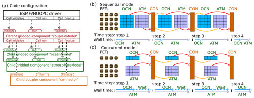
Figure 2 The general code structure and run sequence of the coupled ocean–atmosphere model. In panel (a), the black block is the application driver; the red block is the parent gridded component called by the application driver; the green (brown) blocks are the child gridded (coupler) components called by the parent gridded component. Panels (b) and (c) show the sequential and concurrent mode implemented in SKRIPS, respectively. PETs (persistent execution threads) are single processing units (e.g., CPU or GPU cores) defined by ESMF. Abbreviations OCN, ATM, and CON denote oceanic component, atmospheric component, and connector component, respectively. The blocks under PETs are the CPU cores in the simulation; the small blocks under OCN or ATM are the small subdomains in each core; the block under CON is the coupler. The red arrows indicate that the model components are sending data to the connector and the yellow arrows indicate that the model components are reading data from the connector. The horizontal arrows indicate the time axis of each component and the ticks on the time axis indicate the coupling time steps.

2.3 The atmospheric component (WRF)

The Weather Research and Forecasting (WRF) model (Skamarock et al., 2019) is developed by the NCAR/MMM (Mesoscale and Microscale Meteorology division, National Center for Atmospheric Research). It is a 3-D finite-difference atmospheric model with a variety of physical parameterizations of subgrid-scale processes for predicting a broad spectrum of applications. WRF is used extensively for operational forecasts as well as realistic and idealized dynamical studies. The WRF code and documentation are under continuous development on GitHub (https://github.com/wrf-model/WRF, last access: 26 September 2019).

In the present work, the Advanced Research WRF dynamic version (WRF-ARW, version 3.9.1.1, https://github.com/NCAR/WRFV3/releases/tag/V3.9.1.1, last access: 26 September 2019) is used. It solves the compressible Euler nonhydrostatic equations and also includes a runtime hydrostatic option. The WRF-ARW uses a terrain-following hydrostatic pressure coordinate system in the vertical direction and utilizes the Arakawa C grid. WRF incorporates various physical processes including microphysics, cumulus parameterization, planetary boundary layer, surface layer, land surface, and longwave and shortwave radiation, with several options available for each process.

Similar to the implementations in MITgcm, WRF is also separated into initialization, run, and finalization subroutines to enable the WRF–ESMF interface to control the atmosphere model during the coupled simulation, shown in Fig. 2a. The implementation of the present WRF–ESMF interface is based on the prototype interface (Henderson and Michalakes, 2005). In the present work, the prototype WRF–ESMF interface is updated to modern versions of WRF-ARW and ESMF, based on the NUOPC layer. This prototype interface is also expanded to interact with the ESMF/NUOPC coupler to receive the oceanic surface variables and send the atmospheric surface variables. The surface boundary condition fields are registered in the coupler following the NUOPC protocols with timestamps. The WRF grid information is also provided for online re-gridding by ESMF. To carry out the coupled simulation on HPC clusters, the WRF–ESMF interface also runs in parallel via MPI communications.

2.4 ESMF/NUOPC coupler

The coupler is implemented using ESMF version 7.0.0. The ESMF is selected because of its high performance and flexibility for building and coupling weather, climate, and related Earth science applications (Collins et al., 2005; Turuncoglu et al., 2013; Chen and Curcic, 2016; Turuncoglu and Sannino, 2017). It has a superstructure for representing the model and coupler components and an infrastructure of commonly used utilities, including conservative grid remapping, time management, error handling, and data communications.

The general code structure of the coupler is shown in Fig. 2. To build the ESMF/NUOPC driver, a main program is implemented to control an ESMF parent component, which controls the child components. In the present work, three child components are implemented: (1) the oceanic component, (2) the atmospheric component, and (3) the ESMF coupler. The coupler is used here because it performs the two-way interpolation and data transfer (Hill et al., 2004). In ESMF, the model components can be run in parallel as a group of persistent execution threads (PETs), which are single processing units (e.g., CPU or GPU cores) defined by ESMF. In the present work, the PETs are created according to the grid decomposition, and each PET is associated with an MPI process.

The ESMF allows the PETs to run in sequential mode, concurrent mode, or mixed mode (for more than three components). We implemented both sequential and concurrent modes in SKRIPS, shown in Fig. 2b and c. In sequential mode, a set of ESMF gridded and coupler components are run in sequence on the same set of PETs. At each coupling time step, the oceanic component is executed when the atmospheric component is completed and vice versa. On the other hand, in concurrent mode, the gridded components are created and run on mutually exclusive sets of PETs. If one component finishes earlier than the other, its PETs are idle and have to wait for the other component, shown in Fig. 2c. However, the PETs can be optimally distributed by the users to best achieve load balance. In this work, all simulations are run in sequential mode.

In ESMF, the gridded components are used to represent models, and coupler components are used to connect these models. The interfaces and data structures in ESMF have few constraints, providing the flexibility to be adapted to many modeling systems. However, the flexibility of the gridded components can limit the interoperability across different modeling systems. To address this issue, the NUOPC layer is developed to provide the coupling conventions and the generic representation of the model components (e.g., drivers, models, connectors, mediators). The NUOPC layer in the present coupled model is implemented according to consortium documentation (Hill et al., 2004; Theurich et al., 2016), and the oceanic and atmospheric components each have

1. prescribed variables for NUOPC to link the component;

2. the entry point for registration of the component;

3. an InitializePhaseMap which describes a sequence of standard initialization phases, including documenting the fields that a component can provide, checking and mapping the fields to each other, and initializing the fields that will be used;

4. a RunPhaseMap that checks the incoming clock of the driver, examines the timestamps of incoming fields, and runs the component;

5. timestamps on exported fields consistent with the internal clock of the component;

6. the finalization method to clean up all allocations.

The subroutines that handle initialization, running, and finalization in MITgcm and WRF are included in the InitializePhaseMap, RunPhaseMap, and finalization method in the NUOPC layer, respectively.

3 Experiment design and observational datasets

We simulate a series of heat events in the Red Sea region, with a focus on validating and assessing the technical aspects of the coupled model. There is a desire for improved and extended forecasts in this region, and future work will investigate whether a coupled framework can advance this goal. The extreme heat events are chosen as a test case due to their societal importance. While these events and the analysis here may not maximize the value of coupled forecasting, these real-world events are adequate to demonstrate the performance and physical realism of the coupled model code implementation. The simulation of the Red Sea extends from 00:00 UTC 1 June to 00:00 UTC 1 July 2012. We select this month because of the record-high surface air temperature observed in the Mecca region, located 70 km inland from the eastern shore of the Red Sea (Abdou, 2014).

The computational domain and bathymetry are shown in Fig. 3. The model domain is centered at 20^∘ N, 40^∘ E, and the bathymetry is from the 2 min Gridded Global Relief Data (ETOPO2) (National Geophysical Data Center, 2006). WRF is implemented using a horizontal grid of 256×256 points and grid spacing of 0.08^∘. The cylindrical equidistant map (latitude–longitude) projection is used. There are 40 terrain-following vertical levels, more closely spaced in the atmospheric boundary layer. The time step for atmosphere simulation is 30 s, which is to avoid violating the CFL (Courant–Friedrichs–Lewy) condition. The Morrison 2-moment scheme (Morrison et al., 2009) is used to resolve the microphysics. The updated version of the Kain–Fritsch convection scheme (Kain, 2004) is used with the modifications to include the updraft formulation, downdraft formulation, and closure assumption. The Yonsei University (YSU) scheme (Hong et al., 2006) is used for the planetary boundary layer (PBL), and the Rapid Radiation Transfer Model for General Circulation Models (RRTMG; Iacono et al., 2008) is used for longwave and shortwave radiation transfer through the atmosphere. The Rapid Update Cycle (RUC) land surface model is used for the land surface processes (Benjamin et al., 2004). The MITgcm uses the same horizontal grid spacing as WRF, with 40 vertical z levels that are more closely spaced near the surface. The time step of the ocean model is 120 s. The horizontal subgrid mixing is parameterized using nonlinear Smagorinsky viscosities, and the K-profile parameterization (KPP) (Large et al., 1994) is used for vertical mixing processes.

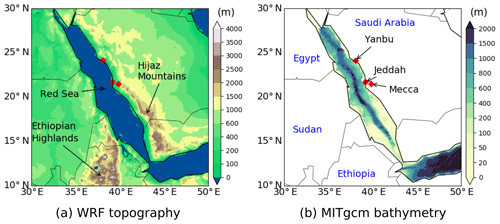
Figure 3 The WRF topography and MITgcm bathymetry in the simulations. Three major cities near the eastern shore of the Red Sea are highlighted. The Hijaz Mountains and Ethiopian Highlands are also highlighted.

During coupled execution, the ocean model sends SST and ocean surface velocity to the coupler, and they are used directly as the boundary conditions in the atmosphere model. The atmosphere model sends the surface fields to the coupler, including (1) surface radiative flux (i.e., longwave and shortwave radiation), (2) surface turbulent heat flux (i.e., latent and sensible heat), (3) 10 m wind speed, (4) precipitation, and (5) evaporation. The ocean model uses the atmospheric surface variables to compute the surface forcing, including (1) total net surface heat flux, (2) surface wind stress, and (3) freshwater flux. The total net surface heat flux is computed by adding latent heat flux, sensible heat flux, shortwave radiation flux, and longwave radiation flux. The surface wind stress is computed by using the 10 m wind speed (Large and Yeager, 2004). The freshwater flux is the difference between precipitation and evaporation. The latent and sensible heat fluxes are computed by using the COARE 3.0 bulk algorithm in WRF (Fairall et al., 2003). In the coupled code, different bulk formulae in WRF or MITgcm can also be used.

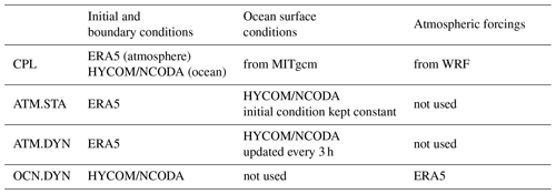
According to the validation tests in the literature (Warner et al., 2010; Turuncoglu et al., 2013; Ricchi et al., 2016), the following sets of simulations using different configurations are performed.

1. Run CPL (coupled run): a two-way coupled MITgcm–WRF simulation. The coupling interval is 20 min to capture the diurnal cycle (Seo et al., 2014). This run tests the implementation of the two-way coupled ocean–atmosphere model.

2. Run ATM.STA: a stand-alone WRF simulation with its initial SST kept constant throughout the simulation. This run allows for assessment of the WRF model behavior with realistic, but persistent, SST. This case serves as a benchmark to highlight the difference between coupled and uncoupled runs and also to demonstrate the impact of evolving SST.

3. Run ATM.DYN: a stand-alone WRF simulation with a varying, prescribed SST based on HYCOM/NCODA reanalysis data. This allows for assessing the WRF model behavior with updated SST and is used to validate the coupled model. It is noted that in practice an accurately evolving SST would not be available for forecasting.

4. Run OCN.DYN: a stand-alone MITgcm simulation forced by the ERA5 reanalysis data. The bulk formula in MITgcm is used to derive the turbulent heat fluxes. This run assesses the MITgcm model behavior with prescribed lower-resolution atmospheric surface forcing and is also used to validate the coupled model.

The ocean model uses the HYCOM/NCODA 1∕12^∘ global reanalysis data as initial and boundary conditions for ocean temperature, salinity, and horizontal velocities (https://www.hycom.org/dataserver/gofs-3pt1/reanalysis, last access: 26 September 2019). The boundary conditions for the ocean are updated on a 3-hourly basis and linearly interpolated between two simulation time steps. A sponge layer is applied at the lateral boundaries, with a thickness of 3 grid cells. The inner and outer boundary relaxation timescales of the sponge layer are 10 and 0.5 d, respectively. In CPL, ATM.STA, and ATM.DYN, we use the same initial condition and lateral boundary condition for the atmosphere. The atmosphere is initialized using the ECMWF ERA5 reanalysis data, which have a grid resolution of approximately 30 km (Hersbach, 2016). The same data also provide the boundary conditions for air temperature, wind speed, and air humidity every 3 h. The atmosphere boundary conditions are also linearly interpolated between two simulation time steps. The lateral boundary values are specified in WRF in the “specified” zone, and the “relaxation” zone is used to nudge the solution from the domain toward the boundary condition value. Here we use the default width of one point for the specific zone and four points for the relaxation zone. The top of the atmosphere is at the 50 hPa pressure level. In ATM.STA, the SST from HYCOM/NCODA at the initial time is used as a constant SST. The time-varying SST in ATM.DYN is also generated using HYCOM/NCODA data. We select HYCOM/NCODA data because the ocean model initial condition and boundary conditions are generated using it. For OCN.DYN we select ERA5 data for the atmospheric state because it also provides the atmospheric initial and boundary conditions in CPL. The initial conditions, boundary conditions, and forcing terms of all simulations are summarized in Table 1.

Table 1 The initial conditions, boundary conditions, and forcing terms used in the simulations.

The validation of the coupled model focuses on temperature, heat flux, and surface wind. Our aim is to validate the coupled model and show that the heat and momentum fluxes simulated by the coupled model are comparable to the observations or the reanalysis data. The simulated 2 m air temperature (T2) fields are validated using ERA5. In addition, the simulated T2 for three major cities near the eastern shore of the Red Sea are validated using ERA5 and ground observations from the NOAA National Climate Data Center (NCDC climate data online at https://www.ncdc.noaa.gov/cdo-web/, last access: 26 September 2019). The simulated SST data are validated against the OSTIA (Operational Sea Surface Temperature and Sea Ice Analysis) system in GHRSST (Group for High Resolution Sea Surface Temperature) (Donlon et al., 2012; Martin et al., 2012). In addition, the simulated SST fields are validated against HYCOM/NCODA data. Since the simulations are initialized using HYCOM/NCODA data, this aims to show the increase in the differences. Surface heat fluxes (e.g., turbulent heat flux and radiative flux), which drive the oceanic component in the coupled model, are validated using MERRA-2 (Modern-Era Retrospective analysis for Research and Applications, version 2) data (Gelaro et al., 2017). We use the MERRA-2 dataset because (1) it is an independent reanalysis dataset compared to the initial and boundary conditions used in the simulations and (2) it also provides $\mathrm{0.625}{}^{\circ }\times \mathrm{0.5}{}^{\circ }$ (long × lat) resolution reanalysis fields of turbulent heat fluxes (THFs). The 10 m wind speed is also compared with MERRA-2 data to validate the momentum flux in the coupled code. The validation of the freshwater flux is shown in the Appendix because (1) the evaporation is proportional to the latent heat in the model and (2) the precipitation is zero in the cities near the coast in Fig. 3. The validation data are summarized in Table 2.

When comparing T2 with NCDC ground observations, the simulation results and ERA5 data are interpolated to the NCDC stations. When interpolating to NCDC stations near the coast, only the data saved on land points are used.³ The maximum and minimum T2 every 24 h from the simulations and ERA5 are compared to the observed daily maximum and minimum T2. On the other hand, when comparing the simulation results with the analysis or reanalysis data (HYCOM, GHRSST, ERA5, and MERRA-2), we interpolate these data onto the model grid to achieve a uniform spatial scale (Maksyutov et al., 2008; Torma et al., 2011).

Table 2 The observational data and reanalysis data used to validate the simulation results.

4 Results and discussions

The Red Sea is an elongated basin covering the area between 12–30^∘ N and 32–43^∘ E. The basin is 2250 km long, extending from the Suez and Aqaba gulfs in the north to the strait of Bab-el-Mandeb in the south, which connects the Red Sea and the Indian Ocean. In this section, the simulation results obtained by using different model configurations are presented to show that SKRIPS is capable of performing coupled ocean–atmosphere simulations. The T2 from CPL, ATM.STA, and ATM.DYN are compared with the validation data to evaluate the atmospheric component of SKRIPS; the SST obtained from CPL and OCN.DYN are compared to validate the atmospheric component of SKRIPS; the surface heat fluxes and 10 m wind are used to assess the coupled system.

4.1 2 m air temperature

We begin our analysis by examining the simulated T2 from the model experiments, aiming to validate the atmospheric component of SKRIPS. Since the record-high temperature is observed in the Mecca region on 2 June, the simulation results on 2 June (36 or 48 h after the initialization) are shown in Fig. 4. The ERA5 data, and the difference between CPL and ERA5 are also shown in Fig. 4. It can be seen in Fig. 4i that CPL captures the T2 patterns in the Red Sea region on 2 June compared with ERA5 in Fig. 4ii. Since the ERA5 T2 data are in good agreement with the NCDC ground observation data in the Red Sea region (detailed comparisons of all stations are not shown), we use ERA5 data to validate the simulation results. The difference between CPL and ERA5 is shown in Fig. 4iii. The ATM.STA and ATM.DYN results are close to the CPL results and thus are not shown, but their differences with respect to ERA5 are shown in Fig. 4iv and v, respectively. Fig. 4vi to x shows the nighttime results after 48 h. It can be seen in Fig. 4 that all simulations reproduce the T2 patterns over the Red Sea region reasonably well compared with ERA5. The mean T2 biases and root mean square errors (RMSEs) over the sea are shown in Table 3. The biases of the T2 are comparable with those reported in other benchmark WRF simulations (Xu et al., 2009; Zhang et al., 2013a; Imran et al., 2018).

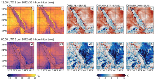
Figure 4 The 2 m air temperature as obtained from the CPL, the ERA5 data, and their difference (CPL−ERA5). The differences between ATM.STA and ATM.DYN with ERA5 (i.e., ATM.STA−ERA5, ATM.DYN−ERA5) are also presented. The simulation initial time is 00:00 UTC 1 June 2012 for both snapshots. Two snapshots are selected: (1) 12:00 UTC 2 June 2012 (36 h from initial time) and (2) 00:00 UTC 3 June 2012 (48 h from initial time). The results on 2 June are presented because the record-high temperature is observed in the Mecca region.

The simulation results on 10 and 24 June are shown in Fig. 5 to validate the coupled model over longer periods of time. It can be seen in Fig. 5 that the T2 patterns in CPL are generally consistent with ERA5. The differences between the simulations (CPL, ATM.STA, and ATM.DYN) and ERA5 show that the T2 data on land are consistent for all three simulations. However, the T2 data over the sea in CPL have smaller mean biases and RMSEs compared to ATM.STA, also shown in Table 3. Although the difference in T2 is very small compared with the mean T2 (31.92 ^∘C), the improvement of the coupled run on the 24 June (1.02 ^∘C) is comparable to the standard deviation of T2 (1.64 ^∘C). The T2 over the water in CPL is closer to ERA5 because MITgcm in the coupled model provides a dynamic SST which influences T2. On the other hand, when comparing CPL with ATM.DYN, the mean difference is smaller (10: +0.04 ^∘C; 24: −0.62 ^∘C). This shows that CPL is comparable to ATM.DYN, which is driven by an updated warming SST.

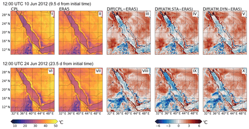
Figure 5 The T2 obtained in CPL, the T2 in ERA5, and their difference (CPL−ERA5). The difference between ATM.STA and ATM.DYN with ERA5 data (i.e., ATM.STA−ERA5, ATM.DYN−ERA5) are also presented. The simulation initial time is 00:00 UTC 1 June 2012 for both snapshots. Two snapshots are selected: (1) 12:00 UTC 10 June 2012 (9.5 d from initial time) and (2) 12:00 UTC 24 June 2012 (23.5 d from initial time).

Table 3 The biases and RMSEs of T2 simulated in all simulations in comparison with ERA5 data.

The mean biases and RMSEs of T2 over the Red Sea during the 30 d simulation are shown in Fig. 6 to demonstrate the evolution of simulation errors. It can be seen that ATM.STA can still capture the T2 patterns in the first week but it underpredicts T2 by about 2 ^∘C after 20 d because it has no SST evolution. On the other hand, CPL has a smaller bias (−0.60 ^∘C) and RMSE (1.28 ^∘C) compared with those in ATM.STA (bias: −1.19 ^∘C; RMSE: 1.71 ^∘C) during the 30 d simulation as the SST evolution is considered. The ATM.DYN case also has a smaller error compared to ATM.STA and its error is comparable with that in CPL (bias: −0.72 ^∘C; RMSE: 1.31 ^∘C), indicating that the skill of the coupled model is comparable to the stand-alone atmosphere model driven by 3-hourly reanalysis SST. The differences in the mean biases and RMSEs between model outputs and ERA5 data are also plotted in Fig. 6. It can be seen that CPL has smaller error than ATM.STA throughout the simulation. The bias and RMSE between CPL and ATM.DYN are within about 0.5 ^∘C. This shows the capability of the coupled model to perform realistic regional coupled ocean–atmosphere simulations.

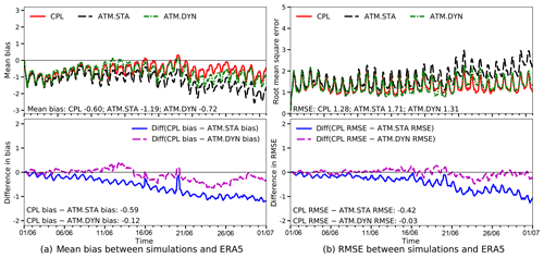
Figure 6 The bias and RMSE between the T2 obtained by the simulations (i.e., ATM.STA, ATM.CPL, and CPL) in comparison with ERA5 data. Only the errors over the Red Sea are considered. The differences between the simulation errors from CPL and stand-alone WRF simulations are presented below the mean bias and the RMSE. The initial time is 00:00 UTC 1 June 2012 for all simulations.

To validate the diurnal T2 variation in the coupled model in Fig. 4, the time series of T2 in three major cities as simulated in CPL and ATM.STA are plotted in Fig. 7, starting from 1 June. The ERA5 data and the daily observed high and low temperature data from NOAA NCDC are also plotted for validation. Both coupled and uncoupled simulations generally captured the four major heat events (i.e., 2, 10, 17, and 24 June) and the T2 variations during the 30 d simulation. For the daily high T2, the RMSE in all simulations are close (CPL: 2.09 ^∘C; ATM.STA: 2.16 ^∘C; ATM.DYN: 2.06 ^∘C), and the error does not increase in the 30 d simulation. For the daily low T2, before 20 June (lead time <19 d), all simulations have consistent RMSEs compared with ground observation (CPL: 4.23 ^∘C; ATM.STA: 4.39 ^∘C; ATM.DYN: 4.01 ^∘C). In Jeddah and Yanbu, CPL has better captured the daily low T2 after 20 June (Jeddah: 3.95 ^∘C; Yanbu: 3.77 ^∘C) than ATM.STA (Jeddah: 4.98 ^∘C; Yanbu: 4.29 ^∘C) by about 1 and 0.5 ^∘C, respectively. However, the T2 difference for Mecca, which is located 70 km from the sea, is negligible (0.05 ^∘C) between all simulations throughout the simulation.

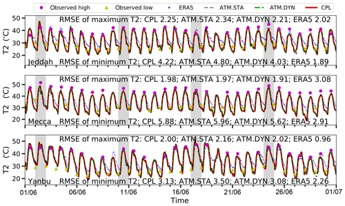
Figure 7 Temporal variation in the 2 m air temperature at three major cities near the eastern shore of Red Sea (Jeddah, Mecca, Yanbu) as resulting from CPL, ATM.STA, and ATM.DYN. The temperature data are compared with the time series in ERA5 and daily high and low temperature in the NOAA national data center dataset. Note that some gaps exist in the NCDC ground observation dataset. Four representative heat events are highlighted in this figure.

4.2 Sea surface temperature

The simulated SST patterns obtained in the simulations are presented to demonstrate that the coupled model can capture the ocean surface state. The snapshots of SST obtained from CPL are shown in Fig. 8i and vi. To validate the coupled model, the SST fields obtained in OCN.DYN are shown in Fig. 8ii and vii, and the GHRSST data are shown in Fig. 8iii and viii. The SST obtained in the model at 00:00 UTC (about 03:00 LT (local time) in the Red Sea region) is presented because the GHRSST is produced with nighttime SST data (Roberts-Jones et al., 2012). It can be seen that both CPL and OCN.DYN are able to reproduce the SST patterns reasonably well in comparison with GHRSST for both snapshots. Though CPL uses higher-resolution surface forcing fields, the SST patterns obtained in both simulations are very similar after 2 d. On 24 June , the SST patterns are less similar, but both simulation results are still comparable with GHRSST (RMSE <1 ^∘C). Both simulations underestimate the SST in the northern Red Sea and overestimate the SST in the central and southern Red Sea on 24 June.

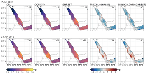
Figure 8 The SST in CPL, OCN.DYN, and GHRSST. The corresponding differences between the simulations and GHRSST are also plotted. Two snapshots of the model outputs are selected: (1) 00:00 UTC 2 June 2012 and (2) 00:00 UTC 24 June 2012. The simulation initial time is 00:00 UTC 1 June 2012 for both snapshots.

To quantitatively compare the errors in SST, the time histories of the SST in the simulations (i.e., OCN.DYN and CPL) and validation data (i.e., GHRSST and HYCOM/NCODA) are shown in Fig. 9. The mean biases and RMSEs between model outputs and validation data are also plotted. In Fig. 9a the snapshots of the simulated SST are compared with available HYCOM/NCODA data every 3 h. In Fig. 9b the snapshots of SST outputs every 24 h at 00:00 UTC (about 03:00 LT local time in the Red Sea region) are compared with GHRSST. Compared with Fig. 9b, the diurnal SST oscillation can be observed in Fig. 9a because the SST is plotted every 3 h. Generally, OCN.DYN and CPL have a similar range of error compared to both validation datasets in the 30 d simulations. The simulation results are compared with HYCOM/NCODA data to show the increase in RMSE in Fig. 9a. Compared with HYCOM/NCODA, the mean differences between CPL and OCN.DYN are small (CPL: 0.10 ^∘C; OCN.DYN: 0.03 ^∘C). The RMSE increases in the first week but does not grow after that. On the other hand, when comparing with GHRSST, the initial SST patterns in both runs are cooler by about 0.8 ^∘C. This is because the models are initialized by HYCOM/NCODA, which has temperature in the topmost model level cooler than the estimated foundation SST reported by GHRSST. After the first 10 d, the difference between GHRSST data and HYCOM/NCODA decreases, and likewise the difference between the simulation results and GHRSST also decreases. It should be noted that the SST simulated by CPL has smaller error (bias: −0.57 ^∘C; RMSE: 0.69 ^∘C) compared with OCN.DYN (bias: −0.66 ^∘C; RMSE: 0.76 ^∘C) by about 0.1 ^∘C when validated using GHRSST. This indicates the coupled model can adequately simulate the SST evolution compared with the uncoupled model forced by ERA5 reanalysis data.

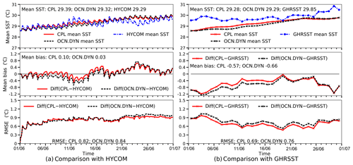
Figure 9 The bias and RMSE between the SST from the simulations (i.e., OCN.DYN and CPL) in comparison with the validation data. Panel (a) shows the 3-hourly SST obtained in the simulations compared with 3-hourly HYCOM/NCODA data. Panel (b) shows the daily SST at 00:00 UTC (about 03:00 local time in the Red Sea region) obtained in the simulations compared with GHRSST. Both simulations are initialized at 00:00 UTC 1 June 2012.

4.3 Surface heat fluxes

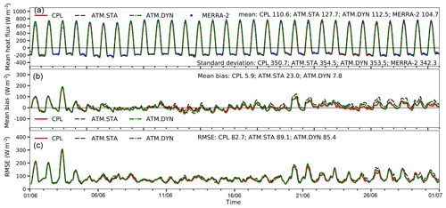
The atmospheric surface heat flux drives the oceanic component in the coupled model, hence we validate the heat fluxes in the coupled model as compared to the stand-alone simulations. Both the turbulent heat fluxes and the net downward heat fluxes are compared to MERRA-2 and their differences are plotted. To validate the coupled ocean–atmosphere model, we only compare the heat fluxes over the sea.

The turbulent heat fluxes (THF; sum of latent and sensible heat fluxes) and their differences with the validation data are shown in Fig. 10 (the snapshots are shown in the Appendix). It can be seen that all simulations have similar mean THF over the Red Sea compared with MERRA-2 (CPL: 119.4 W m⁻²; ATM.STA: 103.4 W m⁻²; ATM.DYN: 117.5 W m⁻²; MERRA-2: 115.6 W m⁻²). For the first 2 weeks, the mean THFs obtained in all simulations are overlapping in Fig. 10. This is because all simulations are initialized in the same way, and the SST in all simulations are similar in the first 2 weeks. After the second week, CPL has smaller error (bias: −1.8 W m⁻²; RMSE: 69.9 W m⁻²) compared with ATM.STA (bias: −25.7 W m⁻²; RMSE: 76.4 W m⁻²). This is because the SST is updated in CPL and is warmer compared with ATM.STA. When forced by a warmer SST, the evaporation increases (also see the Appendix) and thus the latent heat fluxes increase. On the other hand, the THFs in CPL are comparable with ATM.DYN during the 30 d run (bias: 1.9 W m⁻²), showing that SKRIPS can capture the THFs over the Red Sea in the coupled simulation.

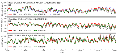
Figure 10 The turbulent heat fluxes out of the sea obtained in CPL, ATM.STA, and ATM.DYN in comparison with MERRA-2. Panel (a) shows the mean THF; (b) shows the mean bias; (c) shows the RMSE. Only the hourly heat fluxes over the sea are shown.

The net downward heat fluxes (sum of THF and radiative flux) are shown in Fig. 11 (the snapshots are shown in the Appendix). Again, for the first 2 weeks, the heat fluxes obtained in ATM.STA, ATM.DYN, and CPL are overlapping. This is because all simulations are initialized in the same way, and the SSTs in all simulations are similar in the first 2 weeks. After the second week, CPL has slightly smaller error (bias: 11.2 W m⁻²; RMSE: 84.4 W m⁻²) compared with the ATM.STA simulation (bias: 36.5 W m⁻²; RMSE: 94.3 W m⁻²). It should be noted that the mean bias and RMSE of the net downward heat fluxes can be as high as a few hundred watts per square meter or 40 % compared with MERRA-2. This is because WRF overestimated the shortwave radiation in the daytime (the snapshots are shown in the Appendix). However, the coupled model still captures the mean and standard deviation of the heat flux compared with MERRA-2 data (CPL mean: 110.6 W m⁻², standard deviation: 350.7 W m⁻²; MERRA-2 mean 104.7 W m⁻², standard deviation 342.3 W m⁻²). The overestimation of shortwave radiation by the RRTMG scheme is also reported in other validation tests in the literature under all-sky conditions due to the uncertainty in cloud or aerosol (Zempila et al., 2016; Imran et al., 2018). Although the surface heat flux is overestimated in the daytime, the SST over the Red Sea is not overestimated (shown in Sect. 4.2).

Figure 11 The total surface heat fluxes into the sea obtained in CPL, ATM.STA, and ATM.DYN in comparison with MERRA-2. Panel (a) shows the mean surface heat flux; (b) shows the mean bias; (c) shows the RMSE. Only the heat fluxes over the sea are shown.

4.4 10 m wind speed

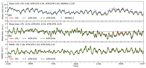
To evaluate the simulation of the surface momentum by the coupled model, the 10 m wind speed patterns obtained from ATM.STA, ATM.DYN, and CPL are compared to the MERRA-2 reanalysis.

The simulated 10 m wind velocity fields are shown in Fig. 12. The RMSE of the wind speed between CPL and MERRA-2 data is 2.23 m s⁻¹ when using the selected WRF physics schemes presented in Sect. 3. On 2 June, high wind speeds are observed in the northern and central Red Sea, and both CPL and ATM.STA capture the features of the wind speed patterns. On 24 June, high wind speeds are observed in the central Red Sea and are also captured by both CPL and ATM.STA. The mean 10 m wind speed over the Red Sea in ATM.STA, ATM.DYN, and CPL during the 30 d simulation are shown in Fig. 13. The mean error of CPL (mean bias: −0.23 m s⁻¹; RMSE: 2.38 m s⁻¹) is slightly smaller than the ATM.STA (mean bias: −0.34 m s⁻¹; RMSE: 2.43 m s⁻¹) by about 0.1 m s⁻¹. Although CPL, ATM.STA, and ATM.DYN have different SST fields as the atmospheric boundary condition, the 10 m wind speed fields obtained in the simulations are all consistent with MERRA-2 data. The comparison shows SKRIPS is capable of simulating the surface wind speed over the Red Sea in the coupled simulation.

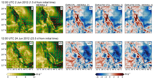
Figure 12 The magnitude and direction of the 10 m wind obtained in the CPL, the MERRA-2 data, and their difference (CPL−MERRA-2). The differences between ATM.STA and ATM.DYN with MERRA-2 (i.e., ATM.STA−MERRA-2, ATM.DYN−MERRA-2) are also presented. Two snapshots are selected: (1) 12:00 UTC 2 June 2012 and (2) 12:00 UTC 24 June 2012.

Figure 13 The magnitude of the 10 m wind obtained in CPL, ATM.STA, and ATM.DYN in comparison with MERRA-2. Panel (a) shows the mean 10 m wind; (b) shows the mean bias; (c) shows the RMSE. Only the hourly surface wind fields over the sea are shown to validate the coupled model.

5 Scalability test

Parallel efficiency is crucial for coupled ocean–atmosphere models when simulating large and complex problems. In this section, the parallel efficiency in the coupled simulations is investigated. This aims to demonstrate that (1) the implemented ESMF/NUOPC driver and model interfaces can simulate parallel cases effectively and (2) the ESMF/NUOPC coupler does not add a significant computational overhead. The parallel speed-up of the model is investigated to evaluate its performance for a constant size problem simulated using different numbers of CPU cores (i.e., strong scaling). Additionally, the CPU time spent on oceanic and atmospheric components of the coupled model is detailed. The test cases are run in sequential mode. The parallel efficiency tests are performed on the Shaheen-II cluster at KAUST (https://www.hpc.kaust.edu.sa/, last access: 26 September 2019). The Shaheen-II cluster is a Cray XC40 system composed of 6174 dual-socket compute nodes based on 16-core Intel Haswell processors running at 2.3 GHz. Each node has 128 GB DDR4 memory running at 2300 MHz. Overall the system has a total of 197 568 CPU cores (6174 nodes $\times \mathrm{2}\times \mathrm{16}$ CPU cores) and has a theoretical peak speed of 7.2 petaflops (10¹⁵ floating point operations per second).

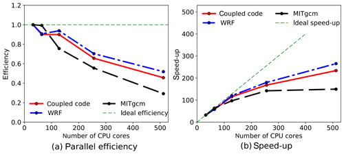
Figure 14 The parallel efficiency test of the coupled model in the Red Sea region, employing up to 512 CPU cores. The simulation using 32 CPU cores is regarded as the baseline case when computing the speed-up. Tests are performed on the Shaheen-II cluster at KAUST.

The parallel efficiency of the scalability test is N_p0t_p0∕N_pnt_pn, where N_p0 and N_pn are the numbers of CPU cores employed in the baseline case and the test case, respectively; t_p0 and t_pn are the CPU times spent on the baseline case and the test case, respectively. The speed-up is defined as t_p0∕t_pn, which is the relative improvement of the CPU time when solving the problem. The scalability tests are performed by running 24 h simulations for ATM.STA, OCN.DYN, and CPL cases. There are 2.6 million atmosphere cells (256 lat ×256 long ×40 vertical levels) and 0.4 million ocean cells (256 lat ×256 long ×40 vertical levels, but about 84 % of the domain is land and masked out). We started using N_p0=32 because each compute node has 32 CPU cores. The results obtained in the scalability test of the coupled model are shown in Fig. 14. It can be seen that the parallel efficiency of the coupled code is close to 100 % when employing less than 128 cores and is still as high as 70 % when using 256 cores. When using 256 cores, there are a maximum of 20 480 cells (16 lat ×16 long ×80 vertical levels) in each core. The decrease in parallel efficiency results from the increase of communication time, load imbalance, and I/O (read and write) operation per CPU core (Christidis, 2015). From results reported in the literature, the parallel efficiency of the coupled model is comparable to other ocean-alone or atmosphere-alone models with similar numbers of grid points per CPU core (Marshall et al., 1997; Zhang et al., 2013b).

Table 4 Comparison of CPU time spent on coupled and stand-alone runs. The CPU time presented in the table is normalized by the time spent on the coupled run using 512 CPU cores. The CPU time spent on two stand-alone simulations are presented to show the difference between coupled and stand-alone simulations.

The CPU time spent on different components of the coupled run is shown in Table. 4. The time spent on the ESMF coupler is obtained by subtracting the time spent on oceanic and atmospheric components from the total time of the coupled run. The most time-consuming process is the atmosphere model integration, which accounts for 85 % to 95 % of the total. The ocean model integration is the second-most time-consuming process, which is 5 % to 11 % of the total computational cost. If an ocean-only region was simulated, the costs of the ocean and atmosphere models would be more equal compared with the Red Sea case. It should be noted that the test cases are run in sequential mode, and the cost breakdown among the components can be used to address load balancing in the concurrent mode. The coupling process takes less than 3 % of the total cost in the coupled runs using different numbers of CPU cores in this test. Although the proportion of the coupling process in the total cost increases when using more CPU cores, the total time spent on the coupling process is similar. The CPU time spent on two uncoupled runs (i.e., ATM.STA, OCN.DYN) is also shown in Table 4. Compared with the uncoupled simulations, the ESMF–MITgcm and ESMF–WRF interfaces do not increase the CPU time in the coupled simulation. In summary, the scalability test results suggest that the ESMF/NUOPC coupler does not add significant computational overhead when using SKRIPS in the coupled regional modeling studies.

6 Conclusion and Outlook

This paper describes the development of the Scripps–KAUST Regional Integrated Prediction System (SKRIPS). To build the coupled model, we implement the coupler using ESMF with its NUOPC wrapper layer. The ocean model MITgcm and the atmosphere model WRF are split into initialize, run, and finalize sections, with each of them called by the coupler as subroutines in the main function.

The coupled model is validated by using a realistic application to simulate the heat events during June 2012 in the Red Sea region. Results from the coupled and stand-alone simulations are compared to a wide variety of available observational and reanalysis data. We focus on the comparison of the surface atmospheric and oceanic variables because they are used to drive the oceanic and atmospheric components in the coupled model. From the comparison, results obtained from various configurations of coupled and stand-alone model simulations all realistically capture the surface atmospheric and oceanic variables in the Red Sea region over a 30 d simulation period. The coupled system gives equal or better results compared with stand-alone model components. The 2 m air temperature in three major cities obtained in CPL and ATM.DYN are comparable and better than ATM.STA. Other surface atmospheric fields (e.g., 2 m air temperature, surface heat fluxes, 10 m wind speed) in CPL are also comparable with ATM.DYN and better than ATM.STA over the simulation period. The SST obtained in CPL is also better than that in OCN.DYN by about 0.1 ^∘C when compared with GHRSST.

The parallel efficiency of the coupled model is examined by simulating the Red Sea region using increasing numbers of CPU cores. The parallel efficiency of the coupled model is consistent with that of the stand-alone ocean and atmosphere models using the same number of cores. The CPU time associated with different components of the coupled simulations shows that the ESMF/NUOPC driver does not add a significant computational overhead. Hence the coupled model can be implemented for coupled regional modeling studies on HPC clusters with comparable performance as that attained by uncoupled stand-alone models.

The results presented here motivate further studies evaluating and improving this new regional coupled ocean–atmosphere model for investigating dynamical processes and forecasting applications. This regional coupled forecasting system can be improved by developing coupled data assimilation capabilities for initializing the forecasts. In addition, the model physics and model uncertainty representation in the coupled system can be enhanced using advanced techniques, such as stochastic physics parameterizations. Future work will involve exploring these and other aspects for a regional coupled modeling system suited for forecasting and process understanding.

Appendix A: Snapshots of heat fluxes

To examine the modeling of turbulent heat fluxes and radiative fluxes, the snapshots of these heat fluxes obtained from ATM.STA, ATM.DYN, and CPL are presented and validated using the MERRA-2 data.

The snapshots of the THFs at 12:00 UTC 2 and 24 June are presented in Fig. A1. It can be seen that all simulations reproduce the THFs reasonably well in comparison with MERRA-2. On 2 June, all simulations exhibit similar THF patterns. This is because all simulations have the same initial conditions, and the SST fields in all simulations are similar within 2 d. On the other hand, for the heat event on 24 June, CPL and ATM.DYN exhibit more latent heat fluxes coming out of the ocean (170 and 153 W m⁻²) than those in ATM.STA (138 W m⁻²). The mean biases in CPL, ATM.DYN, and ATM.STA are 23.1, 5.1, and −9.5 W m⁻², respectively. Although CPL has larger bias at the snapshot, the averaged bias and RMSE in CPL are smaller (shown in Fig. 10). Compared with the latent heat fluxes, the sensible heat fluxes in the Red Sea region are much smaller in all simulations (about 20 W m⁻²). It should be noted that MERRA-2 has unrealistically large sensible heat fluxes in the coastal regions because the land points contaminate the values in the coastal region (Kara et al., 2008; Gelaro et al., 2017), and thus the heat fluxes in the coastal regions are not shown.

The net downward shortwave and longwave radiation fluxes are shown in Fig. A2. Again, all simulations reproduce the shortwave and longwave radiation fluxes reasonably well. For the shortwave heat fluxes, all simulations show similar patterns on both 2 and 24 June. The total downward heat fluxes, which is the sum of the results in Figs. A1 and A2, are shown in Fig. A3. It can be seen that the present simulations overestimate the total downward heat fluxes on 2 June (CPL: 580 W m⁻²; ATM.STA: 590 W m⁻²; ATM.DYN: 582 W m⁻²) compared with MERRA-2 (525 W m⁻²), especially in the southern Red Sea because of overestimating the shortwave radiation. To improve the modeling of shortwave radiation, a better understanding of the cloud and aerosol in the Red Sea region is required (Zempila et al., 2016; Imran et al., 2018). Again, the heat fluxes in the coastal regions are not shown because of the inconsistency of land–sea mask. Overall, the comparison shows the coupled model is capable of capturing the surface heat fluxes into the ocean.

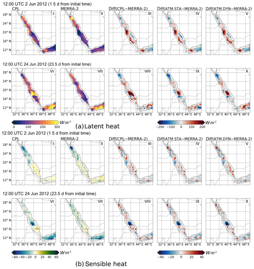
Figure A1 The turbulent heat fluxes out of the sea obtained in CPL, MERRA-2 data, and their difference (CPL−MERRA-2). The differences between ATM.STA and ATM.DYN with MERRA-2 (i.e., ATM.STA−MERRA-2, ATM.DYN−MERRA-2) are also presented. Two snapshots are selected: (1) 12:00 UTC 2 June 2012 and (2) 12:00 UTC 24 June 2012. The simulation initial time is 00:00 UTC 1 June 2012 for both snapshots. Only the heat fluxes over the sea are shown to validate the coupled model.

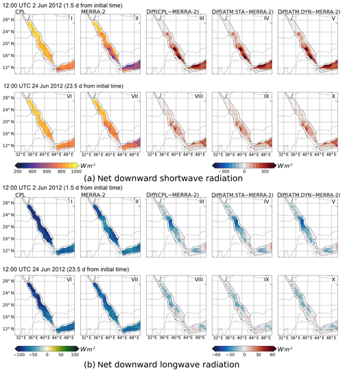
Figure A2 The net downward shortwave and longwave radiation obtained in CPL, MERRA-2 data, and their difference (CPL−MERRA-2). The differences between ATM.STA and ATM.DYN with MERRA-2 (i.e., ATM.STA−MERRA-2, ATM.DYN−MERRA-2) are also presented. Two snapshots are selected: (1) 12:00 UTC 2 June 2012 and (2) 12:00 UTC 24 June 2012. The simulation initial time is 00:00 UTC 1 June 2012 for both snapshots. Only the heat fluxes over the sea are shown to validate the coupled model.

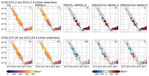
Figure A3 Comparison of the total downward heat fluxes obtained in CPL, MERRA-2 data, and their difference (CPL−MERRA-2). The differences between ATM.STA and ATM.DYN with ERA5 (i.e., ATM.STA−MERRA-2, ATM.DYN−MERRA-2) are also presented. Two snapshots are selected: (1) 1200 UTC 2 June 2012 and (2) 12:00 UTC 24 June 2012. The simulation initial time is 00:00 UTC 1 June 2012 for both snapshots. Only the heat fluxes over the sea are shown to validate the coupled model.

Appendix B: Evaporation

To examine the simulation of surface freshwater flux in the coupled model, the surface evaporation fields obtained from ATM.STA, ATM.DYN, and CPL are compared with the MERRA-2 data.

The surface evaporation fields from CPL are shown in Fig. B1. The MERRA-2 data and the difference between CPL and MERRA-2 are also shown to validate the coupled model. The ATM.STA and ATM.DYN simulation results are not shown, but their differences with CPL are also shown in Fig. B1. It can be seen in Fig. B1iii and viii that CPL reproduces the overall evaporation patterns in the Red Sea. CPL is able to capture the relatively high evaporation in the northern Red Sea and the relatively low evaporation in the southern Red Sea in both snapshots, shown in Fig. B1i and vi. After 36 h, the simulation results are close with each other (e.g., the RMSE between CPL and ATM.STA simulation is smaller than 10 cm yr⁻¹). However, after 24 d, CPL agrees better with MERRA-2 (bias: 6 cm yr⁻¹; RMSE: 59 cm yr⁻¹) than ATM.STA (bias: −25 cm yr⁻¹; RMSE: 68 cm yr⁻¹). In addition, the CPL results are consistent with those in ATM.DYN. This shows the coupled ocean–atmosphere simulation can reproduce the realistic evaporation patterns over the Red Sea. Since there is no precipitation in three major cities (Mecca, Jeddah, Yanbu) near the eastern shore of the Red Sea during the month according to NCDC climate data, the precipitation results are not shown.

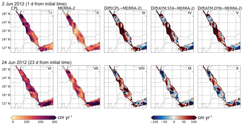
Figure B1 The surface evaporation patterns obtained in CPL, the MERRA-2 data, and their difference (CPL−MERRA-2). The differences between uncoupled atmosphere simulations with MERRA-2 (i.e., ATM.STA−MERRA-2, ATM.DYN−MERRA-2) are also presented. Two snapshots are selected: (1) 12:00 UTC 2 June 2012 and (2) 12:00 UTC 24 June 2012. Only the evaporation over the sea is shown to validate the coupled ocean–Atmosphere model.