the Creative Commons Attribution 4.0 License.
the Creative Commons Attribution 4.0 License.
Dealing with discontinuous meteorological forcing in operational ocean modelling: a case study using ECMWF-IFS and GETM (v2.5)
Meteorological data providers release updated forecasts several times per day – at the forecast epochs. The first time step (t=0) of each forecast, the so-called analysis step, is updated by a data-assimilation process so that the meteorological fields at this time in general do not match the fields from the previous forecast. Seen from the perspective of oceanographic modelling, the analysis step represents a possible discontinuity in the model forcing. Unless care is taken, this “meteorological discontinuity” may generate spurious waves in the ocean model. The problem is examined and quantified for a single meteorological model: the European Centre for Medium-Range Weather Forecasts (ECMWF) Integrated Forecasting System (IFS). A simple straightforward solution is suggested to overcome the forcing discontinuity and the effect on two particular ocean models is examined: the FCOO NA3 (North Atlantic 3 nm) storm-surge model and the NS1C (North Sea–Baltic Sea 1 nm) circulation model.
- Article
(4819 KB) - Full-text XML
- BibTeX
- EndNote
Numerical ocean models are in operational use at many institutions around the world. In the present paper, a particular issue related to an inherent discontinuity of operational meteorological forcing data will be examined. It will be shown that a naïve implementation of an operational forecast process may lead to discontinuous forcing data, which excite spurious waves in the oceanographic model. Further, unless care is taken, there could be a difference in the forcing data applied in, respectively, forecast/nowcast and hindcast modes. This difference may result in under-prediction of forecast/nowcast errors of ocean models.
The discontinuity problem is examined and a straightforward solution is proposed. The effects of the discontinuity on a particular ocean model are quantified and results with and without use of the outlined solution are examined.
2.1 Operational forecast in meteorology
Since the early days of numerical weather prediction (see e.g. Richardson, 1922), observations have played a major role: to accurately forecast the weather systems, an understanding of the near past is necessary. Operational weather forecasts run several times per day using data assimilation schemes to update the initial field in a so-called “analysis step”, e.g. see Lynch (2008). The specific methods used during the analysis are beyond the scope of the present work, but see, for example, Buizza et al. (2005) for a comparison between several weather centres. As we shall see, the data provided for the downstream users are significantly impacted by the assimilation and the analysis step so ocean modellers should be aware of the consequences and take appropriate actions to deal with possible adverse effects.
As part of the optional boundaries programme, the European Centre for Medium-Range Weather Forecasts (ECMWF) provides forecasts every 6 h at times which in the following will be denoted the “epoch” (time zero) of each forecast. Each forecast consists of a number of hourly fields (time steps), delivered in GRIB1 format to the member countries. For each forecast, the simulated time may be denoted by the number of hours from the epoch. Thus, +6 h corresponds to the time of the following epoch (the base time of the next or coming forecast), while −6 h is the previous epoch. As each forecast is significantly longer than 6 h, the initial fields of a forecast coincide in time with fields from several previous forecasts. The meteorological update cycle of hourly fields provided every 6 h is used in illustrations and discussions in the present work. Even so, the results of the present work should be applicable to other update cycles as well.
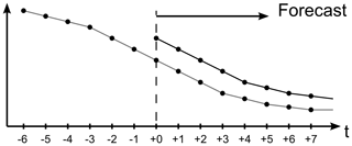
Figure 1Conceptual time series of meteorological data in a particular point for two consecutive forecasts: new (black line) and old (grey). Dots denote times where data fields are available. The actual variable could be, for example, pressure, temperature, or wind. The dashed line denotes the start of the meteorological forecast: +0 h, i.e. the analysis time.
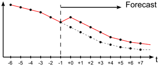
In Fig. 1, it is illustrated how a meteorological forecast differs from the previous forecast at a specific point. The difference is caused by the aforementioned data assimilation procedure in the meteorological forecasting system, which adjusts the forecasts according to observations and updates, e.g. the location of low-pressure areas. In the present work, the change from previous to new forecast at t=0 will be denoted “the meteorological discontinuity” or simply “the jump”. Some atmospheric models are adjusted within a short time window while others (e.g. 4DVAR) provide a smooth transition from the previous forecast to the current forecast in an assimilation window prior to the analysis time or epoch. It is, however, common practice to only disseminate forecasts from the analysis time and forward in time as illustrated in the figure. The dots shown in Fig. 1 thus represent the data actually available for downstream use, e.g. as forcing in oceanographic forecasting models.
2.2 Operational oceanographic forecasting
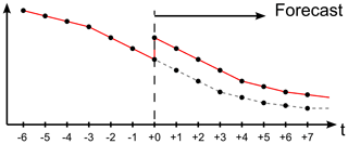
Figure 2Conceptual example of meteorological forcing for ocean model with “hotstart” coinciding with the epoch. It is assumed that the ocean model uses linear interpolation between the available meteorological fields.
Operational ocean models are forced with meteorological forecast data received at each epoch. The ocean models typically run when the meteorological forecasts are available. However, the method for providing initial conditions to the subsequent forecast is rarely documented. It does, however, seem common to keep so-called “hotstart files” with the model state exactly at the analysis time and then at time +6 h save new hotstart files needed for the next epoch. At a first glance, this choice of hotstart time may seem natural. However, as discussed, the meteorological data from two consecutive forecasts are discontinuous exactly at the epoch – the analysis time. Therefore, even though there is a high correlation between the current and previous forecasts, each meteorological forecast should be seen as an entirely new forcing function for the ocean model rather than an extension of the previous forcing function, see Fig. 2.
If the ocean model hotstart time is chosen to coincide with the analysis time, then effectively the ocean model is forced by meteorological fields from the previous forecast (grey line in Fig. 1) up until the epoch and by new or updated fields after the epoch (black line in Fig. 1). Even though the ocean model may interpolate (linearly) in time between the available meteorological fields, the forcing is discontinuous exactly at the epoch. This discontinuity in the meteorological forcing, which could include instantaneous repositioning of pressure minima, may generate non-physical waves as the ocean model adapts to the sudden changes in forcing. Since this process is repeated every 6 h (every epoch), the ocean model is in effect forced by discontinuous data every 6 h back in time and these discontinuities may generate spurious non-physical waves that propagate around the model domain.
It can be seen from Fig. 2 that time −1 h is the last meteorological field which is not changed by the new forecast. Thus, to avoid the discontinuity, the ocean model should really employ temporal interpolation from −1 h (using data from the previous forecast) to +0 h of the new forecast. However, as the new data for +0 h is not available at the time of the previous ocean forecast, the new ocean forecast must start at −1 h, see Fig. 3. As a consequence, the hotstart files for the next forecast must be written at +5 h; 6 h of simulated time into the forecast. This approach corresponds exactly to running a hindcast based on the first six (hourly) fields of each meteorological forecast, which – for hindcasts – seems to be a very common choice among ocean modellers. Modellers running hindcasts according to this model (Fig. 3) and operational forecasts according to the previous (Fig. 2) should be aware of the difference. In such cases, the hindcasts could under-predict the errors in the model leading to too high confidence in an operational model, when compared to the model in a hindcast scenario.
At the Joint GeoMETOC Support Center (FCOO), the ocean forecast always starts at −1 h to avoid discontinuities of the meteorological forcing. The extra simulated hour is only a small overhead to pay for the increased model accuracy which follows. Also, for hindcast simulations, FCOO use the same meteorological forcing principles as the operational model (excepting the forecast period itself), such that the hindcast performance may be used as a solid base for operational performance of at least the first 5–6 h of the forecast.
2.3 Ramping
Even if hotstarts are positioned at −1 h, it is not ensured that the meteorological forcing is smooth, see Fig. 3. Although the severe discontinuity is avoided, the epoch can still represent an hour with larger changes in meteorology than a typical hour of the simulation. As a result there may still be generated unphysical waves in the ocean model – although hopefully at a smaller scale. To increase the uniformity of the meteorological forcing, it is possible to perform a so-called ramping process in which a linear combination between old and new meteorological forecast fields are used to change smoothly from the old to the new forecasts. If denotes the nth field of forecast no. i so that and are consecutive forecasts for meteorological fields at the same time (hour on the clock), then the “rampN” process computes updated fields as
For N>6, i.e. if the ramping is longer then the number of time fields between consecutive forecasts, it is necessary to make the computation recursive so that Eq. (1) is used for the first ramping (i=1), while later epochs use in place of . The method is outlined in Fig. 4 for different values of the ramping length. It should be noted that the suggested ramping process does not imply interpolation in time.
The obvious disadvantage is that the ramping process sacrifices the accuracy of the first fields of the meteorological forecast by replacing a significant part of the data with older and probably less accurate data from the previous forecast. Thus, the ramping is a delicate balance between smoothness and (local) accuracy. As is the case in many other aspects of (ocean) modelling, such as the bathymetry, the use of the most accurate (unfiltered) data does not implicitly ensure the most accurate results.
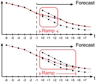
Figure 4Conceptual examples of meteorological forcing for ocean model with hotstart at −1 h and 3 or 6 h of meteorological ramping. Longer ramping yields smoother transition between old and new forecast data.
While the ramping process of meteorological forcing data requires some preprocessing overhead, there is no computational penalty involved for the actual model forecasting. It should be noted that it is entirely possible to use a ramp longer than the time between epochs.
Note that the initial shifting of the hotstart time shown in Fig. 3 may be considered a special case of the ramping procedure. If “rampN” denotes ramping over N meteorological fields, such that Fig. 4 shows ramp3 and ramp6, then Fig. 3 shows ramp0, i.e. a linear interpolation between old and new forecasts but with no intermediate interpolated fields. The discontinuous process shown in Fig. 2 could then be dubbed “no ramping” (noramp).
It should be noted that if two consecutive meteorological forecasts provide very similar results, i.e. if the discontinuity is small, then the effect of ramping is also small. In essence, the suggested ramping process is not harmful in general but kicks in when the discontinuity is significant.
At the Joint GeoMETOC Support Center (FCOO) all meteorological forcing data are ramped before being used as forcing for oceanographic models. The ramping length depends on the experience with the particular meteorological dataset. For the ECMWF-IFS data, ramp6 is used operationally at FCOO.
If the weather centres would provide updated information for previous fields (t<0) to present a smooth update from some prior known state to the present analysis time, then that would be preferable to using the presented ramping method. In such a scenario, the hotstart time of the oceanographic model should simply be pushed back in time to the latest unchanged field in a procedure totally equivalent to what is presented in Fig. 3.
2.4 Operational ocean model setup
During each FCOO forecast cycle, three nested setups (Büchmann et al., 2011) of the General Estuarine Transport Model (GETM; see Burchard and Bolding, 2002) are run in sequence, see Fig. 5. The outermost setup (NA3) is a barotropic storm-surge model setup and it feeds inwards to two nested 3-D baroclinic setups (NS1C, DK600).
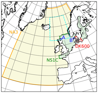
Figure 5FCOO nested GETM ocean model setup: NA3, NS1C, and DK600. Station Wick (A) is used as proxy for effect on boundary conditions for the NS1C model, while station Hanstholm (B) is used to gauge the actual effect on the NS1C model. For later reference the north-east Atlantic area “neatl” (latitudes 58 to 70, longitudes −14 to 6) is marked with a dashed cyan box.
The NA3 setup is a 2-D storm-surge model with no tidal wave components included. The lateral boundary conditions are forced by Flather-style boundary conditions (Carter and Merrifield, 2007) driven by the so-called inverse barometric effect (Ponte et al., 1991) derived from the meteorological forecast from the ECMWF-IFS (Integrated Forecasting System) model. The meteorological wind (stress) and pressure components of the ECMWF-IFS forecast data also act directly on the ocean free surface.
The NS1C and DK600 setups are 3-D baroclinic setups and include tides, which are added to the boundaries of NS1C, where Oregon State University (OSU) tidal data inversion (Egbert and Erofeeva, 2002) data are combined with surface elevations and depth-integrated velocities from the NA3 setup to get elevation and velocity boundary conditions. Data from DMI-HARMONIE-NEA (Bengtsson et al., 2017) are used to force the surface of the NS1C and DK600 setups. As the NA3 setup is used for boundary conditions (nesting), there is an impact from the ECMWF-IFS model on the inner NS1C and DK600 models. Any discontinuities in the meteorological pressure – especially in the “neatl” area shown in Fig. 5 – may propagate to the boundaries of the NS1C setup and thus create non-physical waves in the NS1C and DK600 setups.2
Presently, FCOO makes 54 h forecasts, i.e. to time +54 h, of the entire model complex (NA3-NS1C-DK600) four times per day at epochs 00:00, 06:00, 12:00, and 18:00 UTC. The timing is based on data availability of the meteorological models used for forcing the ocean models.
In this section, the meteorological pressure discontinuity will be examined in detail (Sect. 3.1). Subsequently, the effect on the ocean model will be examined (Sect. 3.2).
3.1 Meteorological forcing
In order to quantify the difference in sea level pressure (SLP) caused by the discontinuity between two meteorological forecasts, the typical SLP change during 1 h of a forecast is computed, see Fig. 6. For each of the four daily IFS forecasts during 2016–2018, the absolute pressure difference between each forecast field and the previous field is computed for each of the first 18 fields (+01 to +18 h). Subsequently, the values are averaged over each forecast (18 fields) and over all 4384 forecasts in the 3-year period. For the “neatl” area near the northern boundary of the NS1C model (see Fig. 5), the average hourly change is computed to 42 Pa.
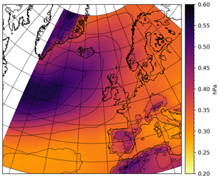
Figure 6ECMWF-IFS absolute hourly pressure change for the first 18 h (+0 h through +18 h) forecast – averaged over all 4384 (four daily) forecasts during 2016–2018. The spatial average over the neatl area (Fig. 5) is 0.42 hPa.
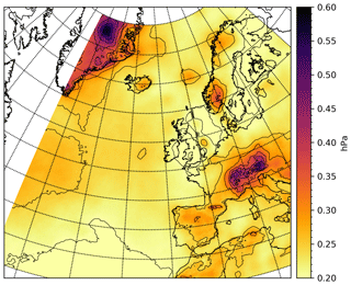
Figure 7ECMWF-IFS absolute pressure discontinuity (jump) averaged over all forecasts during 2016–2018. The spatial average over the neatl area (Fig. 5) is 0.22 hPa.
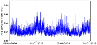
Figure 8Spatial average over the neatl area (Fig. 5) of ECMWF-IFS absolute pressure jump for each forecast during 2016–2018.
The temporal average of the absolute value of the “pressure jump” has been computed, see Fig. 7. For the open ocean, the magnitude is significantly lower than the average hourly pressure change shown in Fig. 6: for the neatl area, the average pressure jump is computed to 0.22 hPa or 54 % of the average hourly change in the same area. In other words, the update to the analysis field corresponds – on average – to about half the typical hourly change. However, the average pressure change of Fig. 7 hides a rather large variability in both time and space. To examine the temporal variation, the spatial average (over the “neatl” area) of the absolute pressure jump has been computed as a function of time for the 3-year period 2016–2018, see Fig. 8. As written previously, the temporal average is 0.22 hPa but this covers a variation exceeding an order of magnitude: from 0.068 to 0.81 hPa, the latter occurring at 24 December 2016 00:00 UTC (all dates and times in this paper are in UTC).
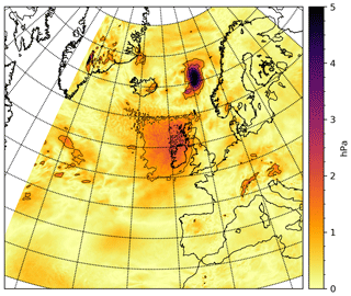
Figure 9ECMWF-IFS absolute pressure jump at 24 December 2016 00:00, i.e. absolute pressure difference between 2016122400+0 h (analysis step) and 2016122318+6 h. The spatial average over the neatl area (Fig. 5) is 0.81 hPa. Note the changed colour scale: the maximum pressure difference is 5.7 hPa, occurring at point 64.793, 0.773 (lat., long.).
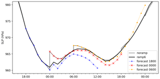
Figure 10First 18 h of ECMWF-IFS surface pressure (SLP) forecasts at point 64.793, 0.773 (lat., long.) for epochs 23 December 2016 18:00 UTC, 24 December 2016 00:00 UTC, and 24 December 2016 06:0 UTC. Also shown are the resulting forcing without use of ramping (noramp) and for a 6 h ramping (ramp6).
If the SLP discontinuity at 24 December 2016 00:00 is examined in detail, see Fig. 9, then it may be seen that the local (in space) pressure jump at that time exceeds 5 hPa. The largest pressure jump appears on the east side of a low-pressure system (results not shown), where the meteorology analysis step apparently has adjusted the size and speed of the system slightly. Overall, however, the two pressure fields (weather maps) do look very similar so there has not been any large error in the pressure forecast.
Time series of SLP for three consecutive forecasts for a single point are depicted in Fig. 10. For comparison, the time series for “noramp” and “ramp6” are also shown. It should be noted that without ramping, the SLP forcing used for a hydrodynamic model does include significant pressure discontinuities. The introduction of ramping (see Sect. 2.3) decreases the spurious pressure jumps significantly. Further, if the pressure jump is small, i.e. if the present and previous forecasts agree, then there is no large impacts from the ramping procedure and thus the noramp and ramp6 methods give essentially the same result. Basically, the adverse effects of the ramping method seem to be small. Even though the impact of best first fields of each forecast are reduced, the change is small unless there are large updates in the analysis step, which is exactly the time where ramping is necessary to alleviate discontinuities in the forcing.
3.2 Impact on ocean model
To investigate how the discontinuity affects the ocean elevation, the ocean models NA3 and NS1C have been run in hindcast mode with different preprocessing (ramping) of the meteorological forcing: noramp, ramp0, and ramp6, see Figs. 2, 3, and 4 for the period 1 December 2016 through 31 December 2018. In all cases, the ocean models have been forced by the ECMWF-IFS dataset, only the ramping method is varied. In operational mode, the NS1C model is forced with meteorological data from the Danish Meteorological Institute (DMI-HARMONIE-NEA) but for simplicity the ECMWF-IFS data are used in the present work.
As seen in the previous section, the pressure discontinuity may in certain situations exceed 5 hPa. As a single hecto-pascal corresponds roughly to 1 cm of water column, spurious waves of the order of several centimetres might be expected. As the discontinuous forcing could excite gravity waves over a range of frequencies, it may be difficult to a priori estimate the spectral content of the spurious waves.
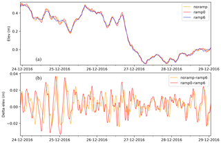
Figure 11NA3 surge elevation at Wick station during December 2016 forced by ECMWF-IFS data. (a) Results for models forced by the “noramp” (discontinuous), “ramp0”, and “ramp6” methods and (b) differences between short ramps and the recommended ramp6.
As a proxy for the impact on the NS1C north boundary, the computed surge elevation at Wick station (see Fig. 5) is examined. 3 The time step (Δt) of the NA3 model is 8 s; to ensure that high-frequency components are resolved and to avoid data aliasing, station data have been saved every 40 s, i.e. every 5 time steps. In Fig. 11, the Wick elevation is depicted for the two cases examined. Also the difference between the two surge time series is shown in the figure. With respect to the overall features – on the scale of several hours to days – the time series of the two methods agree. However, there is significant difference in the higher-frequency components: the elevation difference (Fig. 11b) has significant energy components in the range of 1 to 2 h (results not shown). For the chosen station and period, however, it is not clear if the ramp0 method is significantly better than no ramping. It may be noted that the magnitude of the differences is of the order of several centimetres, consistent with the magnitudes of the pressure discontinuities found in the previous section. At FCOO, the modelled data (elevations, in this case) are routinely compared to observations in order to gauge the performance of the model. For the present setup and station, the RMS error – comparing model elevation to observed surge (low-pass filtered elevation) – has been computed to 6.8 cm for 2016 and 5.1 cm for 2017. In comparison, the pressure discontinuity – inducing changes of up to 3–4 cm for the present station – is by no means the leading error term, but it is not negligible either.
The pressure discontinuity affects the nested model (NS1C) both directly on the free surface and through the boundary conditions computed from the NA3 results. For the NS1C setup, elevation data have been saved every 90 s at more than 250 stations4 throughout the domain. The Hanstholm station in western Skagerrak on the Danish peninsula of Jutland (see Fig. 5) is examined to gauge the effect on a station in the NS1C model setup. While the event in December 2016 results in differences of up to 4–5 cm at the Hanstholm station (results not shown but data available online), a year later the differences exceed 6 cm, corresponding to nearly 5 % of the monthly elevation range, see Fig. 12.
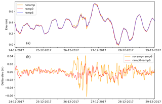
Figure 12NS1C elevation at Hanstholm station during December 2017 forced by ECMWF-IFS data. (a) Results for models forced by the “noramp”, “ramp0”, and “ramp6” methods, and (b) differences between short ramps and the recommended ramp6.
From the figure, it may be noted that the “noramp” method results in high-frequency components in the elevation signal, especially on 26 December 2017. In the present case, the ramp0 method suppresses the major part of the high-frequency components. It is also observed that most of the time the difference between the three methods is small. Compared to observed elevation, the statistics for the Hanstholm station (forced with ECMWF-IFS ramp6) show an RMS error of 6.9 cm for 2016 and 6.4 cm for 2017. Again, the pressure discontinuity is not a leading error term but it should be worth addressing.
For completeness, it should be mentioned that even the slightest change in forcing or initial conditions may induce a change in the location of baroclinic eddies in the 3-D circulation model. Büchmann and Söderkvist (2016) found the related salinity ensemble variability to be less than about 1 PSU in Skagerrak. At any particular time the exact eddy location may differ between the three simulations (noramp, ramp0 and ramp6) and this introduces a small elevation difference, which is unrelated to the pressure jumps. The elevation difference was not examined explicitly for Skagerrak by Büchmann and Söderkvist (2016) but for a station in Kattegat the difference was found to be of the order of 0.1 mm – about 2 orders of magnitude smaller than the effects from the meteorological pressure discontinuities examined in the present work. Thus, the differences shown in Fig. 12b do originate from the pressure discontinuities rather than from repositioning of baroclinic eddies.
Data assimilation in meteorological models – implemented at the so-called “analysis step” – results in updated data fields at this and later time steps. It appears to be common practice that weather centres, such as the European Centre for Medium-Range Weather Forecasts (ECMWF), disseminate updated forecasts only from the forecast epoch (t=0) and forward (t>0). It has been shown that direct use of such meteorological forcing – in combination with saving hotstart files exactly at the epoch – results in the use of a meteorological forcing with a discontinuity at every model epoch back in time.
As a side note, it is observed that the discontinuity may not be present in hindcast mode, and thus the forecast error of an oceanographical model could be under-estimated unless care is taken.
The size of the pressure discontinuity has been examined for a single model: the ECMWF-IFS model in a particular area in the north-east Atlantic. It was found that although the discontinuity on average is only about 0.2 hPa, it may exceed 5 hPa at specific incidents. A simple, straightforward, and easy-to-implement solution to the problem has been suggested, namely to slowly ramp the new forecast data, i.e. to use a linear combination of old and new forecasts for a few time steps.
The effect of the discontinuity on a particular operational storm-surge model has been examined and spurious waves of the magnitude of several centimetres were observed in an area where the storm-surge model data are used as boundary conditions for a higher-resolution operational circulation model. Additionally, it has been shown that high-frequency spurious waves may also be seen directly in the circulation model. For the two particular stations examined, the magnitude of the spurious waves was in the same order of magnitude as the annual RMS error of the model elevation compared to in situ observations. Although the pressure discontinuity – for the present model setups – is not the leading error term, it is considered well worth the effort to eliminate the possible spurious waves in the models.
It is recommended that operational ocean modellers take steps to ensure that the meteorological forcing fields are smooth in time. Preferably, meteorological forcing providers may provide updated forcing fields also before the forecast epoch, i.e. for t<0, thus providing every field which has been updated by the data assimilation procedure. In this case, the ocean model hotstart time should be moved to the time of the latest meteorological field which is not updated by the process. As an alternative, the discontinuity may be alleviated by the ramping procedure suggested in the present work.
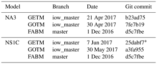
GETM (Burchard and Bolding, 2002, https://getm.eu/) (last access: 30 August 2019) is open source and builds on GOTM (Umlauf and Burchard, 2005, https://gotm.net/) (last access: 30 August 2019) and FABM (Bruggeman and Bolding, 2014, https://github.com/fabm-model/fabm) (last access: 30 August 2019). The source code versions used in the present work reflect the executables in operational use at FCOO at the time of writing. As a consequence, the source codes differ between the NA3 and NS1C model setups. The exact git commit hashes and dates for the code used are given in Table 1.
For operational purposes the GETM code for NS1C was modified slightly to improve the initializations of particular arrays. The modifications do not impact on the results of the present paper. The exact source code – including changes – used in this study is available online at https://doi.org/10.5281/zenodo.3243187 (Büchmann, 2019). The actual changes compared to GETM-25dabf7 are given also as a diff file.
Data used in this article are available online at Zenodo.org, https://doi.org/10.5281/zenodo.3243187 (Büchmann, 2019). The raw data for Figs. 6–12 are available as individual tar balls of NetCDF data files. Model elevation data are available in NetCDF format for 40 station in the NA3 domain and 266 stations in the NS1C domain for the three examined ramp settings for the period 1 December 2016 through 31 December 2018.
ECMWF-IFS data are available through the Meteorological Archive and Retrieval System (MARS), but access is limited to member countries. For the present paper, the first 19 hourly fields of each of four daily operational weather forecasts, 1 January 2016–31 December 2018, have been used.
BB identified the possible discontinuity, suggested the solution, examined the effects, implemented the solution operationally at FCOO, and wrote the paper.
The author declares that there is no conflict of interest.
The author acknowledges fruitful discussions with and feedback from present and previous FCOO colleagues.
This paper was edited by James Annan and reviewed by two anonymous referees.
Bengtsson, L., Andrae, U., Aspelien, T., Batrak, Y., Calvo, J., de Rooy, W., Gleeson, E., Hansen-Sass, B., Homleid, M., Hortal, M., Ivarsson, K.-I., Lenderink, G., Niemelä, S., Nielsen, K. P., Onvlee, J., Rontu, L., Samuelsson, P., Muñoz, D. S., Subias, A., Tijm, S., Tolla, V., Yang, X., and Ødegaard Køltzow, M.: The HARMONIE-AROME Model Configuration in the ALADIN-HIRLAM NWP System, Mon.Weather Rev., 145, 1919–1935, https://doi.org/10.1175/MWR-D-16-0417.1, 2017. a
Bruggeman, J. and Bolding, K.: A general framework for aquatic biogeochemical models, Environ. Modell. Softw., 61, 249–265, https://doi.org/10.1016/j.envsoft.2014.04.002, 2014. a
Büchmann, B.: Dealing with discontinuous meteorological forcing in operational ocean modelling: a case study using ECMWF-IFS and GETM (v2.5) (Version 0.1.1) [Data set], Zenodo, https://doi.org/10.5281/zenodo.3243187, 2019. a, b
Büchmann, B. and Söderkvist, J.: Internal variability of a 3-D ocean model, Tellus A: Dynam. Meteorol. Oceanogr., 68, 30417, https://doi.org/10.3402/tellusa.v68.30417, 2016. a, b
Büchmann, B., Hansen, C., and Söderkvist, J.: Improvement of hydrodynamic forecasting of Danish waters: impact of low-frequency North Atlantic barotropic variations, Ocean Dynam., 61, 1611–1617, https://doi.org/10.1007/s10236-011-0451-2, 2011. a
Buizza, R., Houtekamer, P. L., Toth, Z., Pellerin, G., Wei, M., and Zhu, Y.: A Comparison of the ECMWF, MSC, and NCEP Global Ensemble Prediction Systems, Mon. Weather Rev., 133, 1076–1097, https://doi.org/10.1175/MWR2905.1, 2005. a
Burchard, H. and Bolding, K.: GETM – A general estuarine transport model, Tech. rep., Joint Research Centre, Ispra, 2002. a, b
Carter, G. S. and Merrifield, M. A.: Open boundary conditions for regional tidal simulations, Ocean Modell., 18, 194–209, https://doi.org/10.1016/j.ocemod.2007.04.003, 2007. a
Egbert, G. D. and Erofeeva, S. Y.: Efficient inverse modeling of barotropic ocean tides, J. Atmos. Ocean. Technol., 19, 183–204, https://doi.org/10.1175/1520-0426(2002)019<0183:EIMOBO>2.0.CO;2, 2002. a
Lynch, P.: The origins of computer weather prediction and climate modeling, J. Comput. Phys., 227, 3431–3444, https://doi.org/10.1016/j.jcp.2007.02.034, 2008. a
Ponte, Rui M., Salstein, D. A., and Rosen, R. D.: Sea Level Response to Pressure Forcing in a Barotropic Numerical Model, Ocean Modell., 21, 194–209, https://doi.org/10.1175/1520-0485(1991)021<1043:SLRTPF>2.0.CO;2, 1991. a
Richardson, L. F.: Weather Prediction by Numerical Process, Cambridge University Press, Cambridge, 1922. a
Umlauf, L. and Burchard, H.: Second-order turbulence closure models for geophysical boundary layers. A review of recent work, Conti. Shelf Res., 25, 795–827, https://doi.org/10.1016/j.csr.2004.08.004, 2005. a
“GRIdded Binary or General Regularly-distributed Information in Binary form” defined by the World Meteorological Organization's Manual on Codes No. 306.
As NS1C and DK600 use DMI-HARMONIE-NEA data as forcing, the meteorological discontinuity of this model must be considered as well.
Time series of 40 stations for each of the three ramp settings are available online.
Time series for 266 stations are available online.


