Assessment of wavelet-based spatial verification by means of a stochastic precipitation model (wv_verif v0.1.0)

The quality of precipitation forecasts is difficult to evaluate objectively because images with disjointed features surrounded by zero intensities cannot easily be compared pixel by pixel: any displacement between observed and predicted fields is punished twice, generally leading to better marks for coarser models. To answer the question of whether a highly resolved model truly delivers an improved representation of precipitation processes, alternative tools are thus needed. Wavelet transformations can be used to summarize high-dimensional data in a few numbers which characterize the field's texture. A comparison of the transformed fields judges models solely based on their ability to predict spatial structures. The fidelity of the forecast's overall pattern is thus investigated separately from potential errors in feature location. This study introduces several new wavelet-based structure scores for the verification of deterministic as well as ensemble predictions. Their properties are rigorously tested in an idealized setting: a recently developed stochastic model for precipitation extremes generates realistic pairs of synthetic observations and forecasts with prespecified spatial correlations. The wavelet scores are found to react sensitively to differences in structural properties, meaning that the objectively best forecast can be determined even in cases where this task is difficult to accomplish by naked eye. Random rain fields prove to be a useful test bed for any verification tool that aims for an assessment of structure.

1 Introduction

Typical precipitation fields are characterized by large empty areas, interspersed with patches of complicated structure. Forecasts of such intermittent patterns are difficult to verify because we cannot compare them to the observations in a grid-point-wise manner: if a given rain feature is forecast perfectly, but slightly displaced, point-wise verification will punish the error twice, once at the points where precipitation is missing and once at the points where it was erroneously placed. The correctly predicted structure is not rewarded in any way. Following the advent of high-resolution numerical weather predictions, this effect, known as double penalty (Ebert, 2008), has motivated the introduction of numerous new spatial verification tools.

In a comprehensive review of the field, Gilleland et al. (2009) identified four main strategies that deal with the double penalty problem and supply useful diagnostic information on the nature and gravity of forecast errors. The classification was updated to include an emerging fifth class in Dorninger et al. (2018). Proponents of the first strategy, the so-called neighbourhood approach, attempt to ameliorate the issue via successive application of spatial smoothing filters (Theis et al., 2005; Roberts and Lean, 2008). A second group of researchers including Keil and Craig (2009), Gilleland et al. (2010), and recently Han and Szunyogh (2018) explicitly measure and correct displacement errors by continuously deforming the forecast into the observed field. A third popular approach consists of automatically identifying discrete objects in each field and subsequently comparing the properties of these objects instead of the underlying fields. Examples from this category include the MODE technique of Davis et al. (2006) as well as the SAL technique by Wernli et al. (2008).

The fourth group of spatial verification strategies contains so-called scale-separation techniques, which employ some form of high- and low-pass filters to quantify errors on a hierarchy of scales. A classic example of this family is the wavelet-based intensity-scale score of Casati et al. (2004), which decomposes the difference field between observation and forecast via thresholding and an orthogonal wavelet transformation. The final class newly identified by Dorninger et al. (2018) contains the so-called distance measures, which exploit mathematical metrics between binary images developed for image processing applications. One example is Baddeley's delta metric, which was first employed as a verification tool in Gilleland (2011).

The basic idea of the method presented in this study, which can be classified as a scale-separation technique, is that errors, that neither relate to the marginal distribution nor to the location of individual features, should manifest themselves in the field's spatial covariance matrix. Direct estimates of all covariances would require unrealistically large ensemble data sets or restrictive distributional assumptions. Following a similar approach to scale-separated verification, Marzban and Sandgathe (2009), Scheuerer and Hamill (2015), and Ekström (2016) therefore base their verification on the fields' variograms. The variogram is directly related to the spatial auto-correlations (Bachmaier and Backes, 2011) but can be estimated from a single field under the assumption that pairwise differences between values at two grid points only depend on the distance between those locations (the so-called intrinsic hypothesis of Matheron, 1963). Similarly one could require stationarity of the spatial correlations themselves, in which case the desired information is contained within the field's Fourier transform. Both of these stationarity assumptions may be inadequate in realistic situations where the structure of the data varies systematically across the domain; for example, due to orographic forcing, the distribution of water bodies or persistent circulation features.

Weniger et al. (2017) have suggested an alternative approach based on wavelets. The key result in this context comes from the field of texture analysis, where Eckley et al. (2010) proved that the output of a two-dimensional discrete redundant wavelet transform (RDWT) is directly connected to the spatial covariances. The crucial advantage of their approach is that it merely requires the spatial variation of covariances to be slow, not zero – a property known as local stationarity. After some initial experiments by Weniger et al. (2017), this framework has successfully been applied to the ensemble verification of quantitative precipitation forecasts by Kapp et al. (2018). Their methodology consists of (1) performing the corrected RDWT, following Eckley et al. (2010), to obtain an unbiased estimate of the local wavelet spectra at all grid points, (2) averaging these spectra over space, (3) reducing the dimension of these average spectra via linear discriminant analysis, and (4) verifying the forecast via the logarithmic score.

In this study, we aim to expand on their pioneering work in several ways. Firstly, we argue that the aggregation method of simple spatial averaging is not the only sensible approach. An alternative is introduced which incidentally suggests a compact way of visualizing the results of the RDWT: instead of aggregating in the spatial domain, we first aggregate in the scale domain by calculating the dominant scale at each location. Secondly, we use both kinds of spatial aggregates to introduce a series of new wavelet-based scores. In contrast to Kapp et al. (2018), we consider both the ensemble case and the deterministic task of comparing individual fields while avoiding the need for further data reduction. We furthermore demonstrate how to obtain a well defined sign for the error, indicating whether forecast fields are scaled too small or too large. The experiments performed to study the properties of our scores constitute another main innovation: the recently developed stochastic rain model of Hewer (2018) allows us to set up a controlled yet realistic test bed, where the differences between synthetic forecasts and observations lie solely in the covariances and can be finely tuned at will. In contrast to similar tests performed by Marzban and Sandgathe (2009) and Scheuerer and Hamill (2015), our data are physically consistent and thus bear close resemblance to observed rain fields. Lastly, we consider the choice of mother wavelet in detail, using the rigorous wavelet-selection procedure of Goel and Vidakovic (1995). The sensitivity of all newly introduced scores to the wavelet choice is assessed as well.

The remainder of this paper is structured as follows. The stochastic model of Hewer (2018) is introduced in Sect. 2. Sections 3 and 4 respectively discuss the wavelet transformation and spatial aggregation in detail. The general sensitivity of the wavelet spectra to changes in correlation structure is experimentally tested in Sect. 5. Based on these results, we define several possible deterministic and probabilistic scores in Sect. 6. In a second set of experiments (Sect. 7), we simulate synthetic sets of observations and predictions and test our scores' ability to correctly determine the best forecast. A comprehensive discussion of all results is given in Sect. 8.

2 Data: stochastic rain fields

In order to test whether our methodology can indeed detect structural differences between rain fields, we need a reasonably large rain-like data set whose structure is, to some extent, known a priori. Faced with a similar task, Wernli et al. (2008), Ahijevych et al. (2009), and others have employed purely geometric test cases. While those experiments are educational, we would argue that the simple, regular texture of such data bears too little resemblance with reality to constitute a sensible test case for our purposes. As an alternative, Marzban and Sandgathe (2009) considered Gaussian random fields, which have the advantage that the texture is more interesting and can be changed continuously via the parameters of the correlation model. However, since precipitation is generally known to follow non-Gaussian distributions, the realism of this approach is arguably still lacking.

In this study, we generate a more realistic testing environment using the work of Hewer (2018), who developed a physically consistent stochastic model of precipitation fields based on the moisture budget:

$$\begin{array}{}\text{(1)}& {\displaystyle }P=max\left(E-T-\mathit{v}\cdot \mathrm{\nabla }q-q\mathrm{\nabla }\cdot \mathit{v},\mathrm{0}\right),\end{array}$$

where P denotes precipitation, E is a constant evaporation rate (in practice set to zero without loss of generality), q is the absolute humidity, and $\mathit{v}=(u,v{)}^T$ is the horizontal wind field. The threshold T specifies the percentage of the field with non-zero values, i.e. the base rate. The velocity and its divergence are represented via the two-dimensional Helmholtz decomposition, which reads

$${\displaystyle }\mathit{v}=\mathrm{\nabla }\times \mathrm{\Psi }+\mathrm{\nabla }\mathit{\chi }\Rightarrow \mathrm{\nabla }\cdot \mathit{v}={\mathrm{\nabla }}^{\mathrm{2}}\mathit{\chi },$$

where $\mathrm{\nabla }\times \mathrm{\Psi }:=(-{\partial }_x\mathrm{\Psi },{\partial }_y\mathrm{\Psi }{)}^T$ is the rotation of the streamfunction and χ is the velocity potential. The spatial process of P is thus completely determined by $(\mathrm{\Psi },\mathit{\chi },q{)}^T$, which we model as a multivariate Gaussian random field with zero mean and covariance matrix

$$\begin{array}{}\text{(2)}& \begin{array}{rl}\text{Cov}& \left(({\mathrm{\Psi }}_{\mathit{s}},{\mathit{\chi }}_{\mathit{s}},q_{\mathit{s}}{)}^T,({\mathrm{\Psi }}_{\mathit{t}},{\mathit{\chi }}_{\mathit{t}},q_{\mathit{t}}{)}^T\right)=\\ & {\mathbf{\Sigma }}_{\mathrm{\Psi },\mathit{\chi },q}\cdot M\left(\right|\left|b\right(\mathit{t}-\mathit{s}\left)\right||,\mathit{\nu }).\end{array}\end{array}$$

Here, $\mathit{t},\mathit{s}\in {\mathbb{R}}^{\mathrm{2}}$ are two locations within the 2-D domain and M is the Matérn covariance function. The parameter b governs the scale of the correlations and the smoothness parameter ν determines the differentiability of the paths. The matrix ${\mathbf{\Sigma }}_{\mathrm{\Psi },\mathit{\chi },q}$ is set to unity for our experiments, meaning that the velocity components and humidity are uncorrelated. Preliminary tests have shown that these parameters have negligible effects on the structural properties of the resulting rain fields. The covariances needed to simulate a realization of P via Eq. (1), i.e.

$$\begin{array}{ll}{\displaystyle }\text{Cov}& {\displaystyle }\left({\left[q_{\mathit{s}},\mathrm{\nabla }\cdot q_{\mathit{s}},\mathrm{\nabla }{\mathit{\chi }}_{\mathit{s}}-\mathrm{\nabla }\times {\mathrm{\Psi }}_{\mathit{s}},{\mathrm{\nabla }}^{\mathrm{2}}{\mathit{\chi }}_{\mathit{s}}\right]}^T\right.\\ {\displaystyle }& {\displaystyle }\left.{\left[q_{\mathit{t}},\mathrm{\nabla }\cdot q_{\mathit{t}},\mathrm{\nabla }{\mathit{\chi }}_{\mathit{t}}-\mathrm{\nabla }\times {\mathrm{\Psi }}_{\mathit{t}},{\mathrm{\nabla }}^{\mathrm{2}}{\mathit{\chi }}_{\mathit{t}}\right]}^T\right),\end{array}$$

follow from Eq. (2) by taking the respective mean-square derivatives. In the special case where Ψ, χ, and q are uncorrelated, these three Gaussian fields, as well as the necessary first and second derivatives, can directly be simulated via the RMcurlfree model from the R package RandomFields (Schlather et al., 2013). While the underlying distributions of Ψ, χ and q are Gaussian, the precipitation process, consisting of non-linear combinations of the derived fields, can exhibit non-Gaussian behaviour. For further details, the reader is referred to Hewer et al. (2017), Hewer (2018), and references therein.

Figure 1 Example realizations of the stochastic rain model on a 128×128 grid for various choices of scale b and smoothness ν. The threshold T was chosen such that 20 % of the field has non-zero values.

Figure 1 shows several realizations of P. Here, as in the rest of this study, we have normalized all fields to unit sum, thereby removing any differences in total intensity and allowing us to concentrate on structure alone. We recognize that the model produces realistic-looking rain fields, at least for moderately low smoothness (small ν) and large scales (small values of b). Two important restrictions imposed by Eq. (2) become apparent as well. Firstly, the model is isotropic, meaning that it cannot produce the elongated, linear structures which are typical of frontal precipitation fields. Secondly, covariances are stationary, implying the same texture across the entire domain. An anisotropic extension of this model is theoretically relatively straightforward (replacing the scalar parameter b by a rotation matrix), but the technical implementation remains a non-trivial problem. The search for a non-stationary version is an open research question in its own right.

3 The redundant discrete wavelet transform

The technical core of our methodology consists of projecting the fields onto a series of so-called daughter wavelets ${\mathit{\psi }}_{j,l,\mathit{u}}\left(\mathit{r}\right):{\mathbb{R}}^{\mathrm{2}}\to \mathbb{R}$, which are all obtained from a mother wavelet ψ(r) via scaling by $\mathit{r}\to \mathit{r}/j$, a shift by $\mathit{r}\to \mathit{r}-\mathit{u}$ and rotation in the direction denoted by l. Such wavelet transforms, which generate a series of basis functions from a single mother ψ that is localized in space and frequency, allow for an efficient analysis of non-stationary signals on a hierarchy of scales and have attained great popularity in numerous applications. For a general introduction to the field, we recommend Vidakovic and Mueller (1994) and Addison (2017).

Before we can apply wavelets to our problem, we must choose a mother ψ and decide which values of $\mathit{\{}j,l,\mathit{u}\mathit{\}}$ to allow. Starting with the latter decision and guided by our desire to capture the field's covariance structure, we follow Weniger et al. (2017) and Kapp et al. (2018) in choosing a redundant discrete wavelet transform (RDWT). In this framework, the shift u takes on all possible discrete values, meaning that the daughters are shifted to all locations on the discrete grid. The scale j is restricted to powers of 2 and the daughters have three orientations with $l=\mathrm{1},\mathrm{2},\mathrm{3}$ denoting the horizontal, vertical, and diagonal direction, respectively. The projection onto these daughter wavelets, for which efficient algorithms are implemented in the R package wavethresh (Nason, 2016), transforms a 2^J×2^J field into $\mathrm{3}\times J\times {\mathrm{2}}^J\times {\mathrm{2}}^J$ coefficients, one for each location, scale, and direction. Our decision in favour of the RDWT is motivated by a relevant result proven in Eckley et al. (2010). Let

$$\begin{array}{}\text{(3)}& {\displaystyle }X\left(\mathit{r}\right)=\sum _{\text{all }j,l,\mathit{u}}\underset{\text{weight}}{\underbrace{W_{j,l,\mathit{u}}}}\cdot \underset{\text{daughter}}{\underbrace{{\mathit{\psi }}_{j,l,\mathit{u}}\left(\mathit{r}\right)}}\cdot \underset{\text{noise}}{\underbrace{{\mathit{\xi }}_{j,l,\mathit{u}}}}\end{array}$$

be the so-called two-dimensional locally stationary wavelet process (henceforth LS2W). The random increments ${\mathit{\xi }}_{j,l,\mathit{u}}$ are assumed to be Gaussian white noise. Local stationarity means that X's auto-correlation varies infinitely slowly in the limit of infinitely large domains or, equivalently, infinitely highly resolved versions of a unit-sized domain. This requirement is enforced by certain asymptotic regularity conditions on the weights $W_{j,l,\mathit{u}}$. For all technical details the reader is referred to Eckley et al. (2010); Kapp et al. (2018) present a more condensed summary. The main result of Eckley et al. (2010) states that in the limit of an infinitely high spatial resolution, the autocovariances of X can directly be inferred from the squared weights $|W{|}^{\mathrm{2}}$. In analogy to the Fourier transform, $|W{|}^{\mathrm{2}}$ is referred to as the local wavelet spectrum. Eckley et al. (2010) have furthermore proven that the squared coefficients of X's RDWT constitute a biased estimator of this spectrum: due to the redundancy of the transform, the very large daughter wavelets all contain mostly the same information, leading to spectra which unduly over-emphasize the large scales. The bias is corrected via multiplication by a matrix A⁻¹ which contains the correlations between the ${\mathit{\psi }}_{j,l,\mathit{u}}$ and thus depends only on the choice of ψ and the size and resolution of the domain. Away from the asymptotic limit, this step occasionally introduces negative values to the spectra, which have no physical interpretation and pose some practical challenges in the subsequent steps. Preliminary investigations have shown that the abundance of this negative energy sharply decreases with the smoothness of the wavelet ψ and mostly averages out when mean spectra over the complete domain are considered (cf. Appendix, Fig. A3). Apart from the bias correction, the corrected local spectra also need to be smoothed spatially in order to obtain a consistent estimate. The complete procedure, including the computationally expensive calculation of A⁻¹, is implemented in the R package LS2W (Eckley and Nason, 2011).

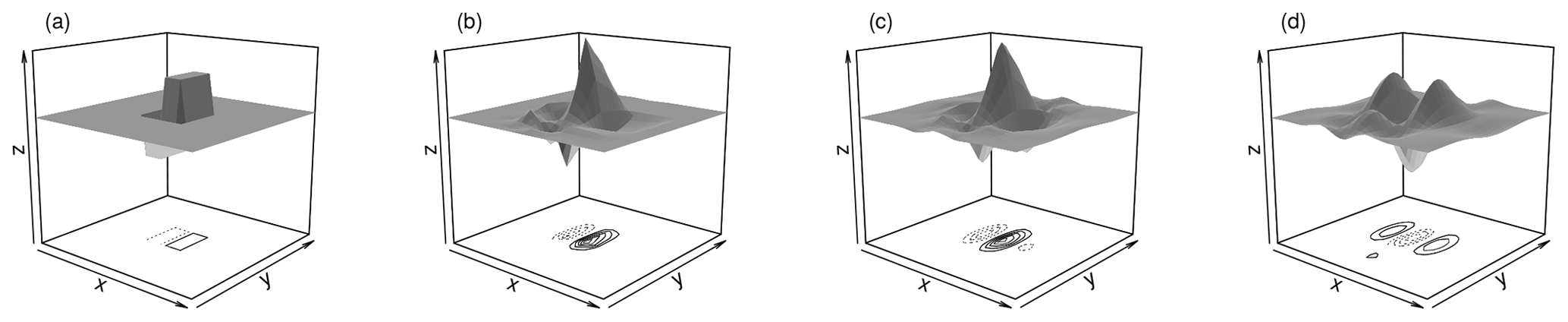
Figure 2 Two-dimensional Daubechies daughter wavelets D₁ and D₂ (a, b), as well as least asymmetric D₄ (c) and D₈ (d), vertical orientation.

Having decided on a type of transformation, we must select a mother wavelet ψ. Our decision is restricted by the fact that the results of Eckley et al. (2010) have only been proven for the family of orthogonal Daubechies wavelets. These widely used functions, henceforth denoted D_N, have compact support in the spatial domain, increasing values of N indicate larger support sizes as well as greater smoothness. Smoother and hence more wave-like basis functions with better frequency localization are thus also more spread out in space. Figure 2 shows a few examples from this family. D₁ (panel a), the only family member that can be written in closed form, is widely known as the Haar wavelet (Haar, 1910) and has been applied in several previous verification studies (Casati et al., 2004; Weniger et al., 2017; Kapp et al., 2018). For N>3, the constraints on smoothness and support length allow for multiple solutions, two of which are typically used: the extremal phase solutions are optimally concentrated near the origin of their support, while the least asymmetric versions have the greatest symmetry (Mallat, 1999). $D_{\mathrm{1},\mathrm{2},\mathrm{3}}$ belongs in both sub-families; wherever a distinction is needed, we will label the two branches of the family as ExP and LeA, respectively. Among these available mother wavelets, we seek the basis that most closely resembles the data, thus justifying the model given in Eq. (3). To this end, we follow Goel and Vidakovic (1995) and rank wavelets by their ability to compress the original data: the sparser the representation (the more of the coefficients are negligibly small) in a given wavelet basis, the greater the similarity between basis functions and data. Relegating all details concerning this procedure to Appendix A, we merely note that the structure of the rain field, determined by the parameters b and ν, has substantially more impact on the efficiency of the compression than the choice of wavelet. Overall, the least asymmetric version of D₄ (shown in Fig. 2c) is most frequently selected as the best basis (28 % of cases), followed by D₁ and D₂ (21 % each). Unless otherwise noted, we will therefore employ LeA4 in all subsequent experiments. Considering the relatively small differences between wavelets, we hypothesize that the basis selection should have only minor effects on the behaviour of the resulting verification measures – a claim which is tested empirically in Sect. 7.

4 Wavelet spectra spatial aggregation

The previous step's redundant transform inflates the data by a factor of 3×J, meaning that a radical dimension reduction is needed before verification can take place. Throughout this study, we will always begin this process by discarding the two largest scales, which are mostly determined by boundary conditions, and averaging over the three directions. The latter step is unproblematic, at least for our isotropic test cases. Next, the resulting fields must be spatially aggregated in a way that eliminates the double-penalty effect.

The straightforward approach to this task consists of simply averaging the wavelet spectra over all locations. The redundancy of the transform guarantees that this mean spectrum is invariant under shifts of the underlying field (Nason et al., 2000), thereby allowing us to circumvent double-penalty effects. Kapp et al. (2018) have already demonstrated that the spatial mean contains enough information to confidently distinguish between weather situations in a realistic setting. In particular, the difference between organized large-scale precipitation and scattered convection has a clear signature in these spectra – an observation that has recently been exploited by Brune et al. (2018), who defined a series of wavelet-based indices of convective organization using this approach. As mentioned above, we furthermore know that negative energy, introduced by the correction matrix A⁻¹, mostly averages out in the spatial mean, provided that we choose a wavelet smoother than D₁ (cf. Appendix, Fig. A3).

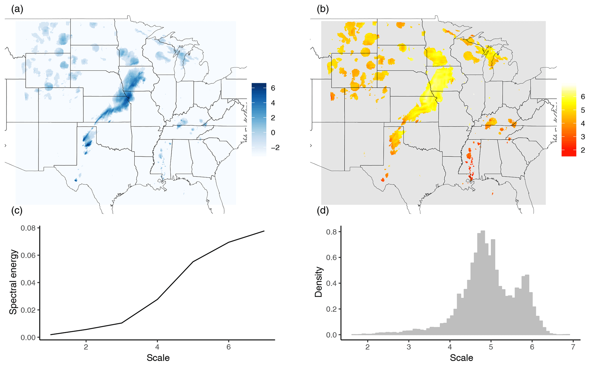
Figure 3 Logarithmic rain field (a) and corresponding map of central scales (b) from the stage II reanalysis on 13 May 2005. The field has been cut and padded with zeroes to 512×512, scales were calculated using the least asymmetric D₄ wavelet, only locations with non-zero rain are shown. Panels (c) and (d) show the corresponding mean spectrum and scale histogram, respectively.

In spite of these desirable properties, there are two main issues which motivate us to consider an alternative way of aggregation: if we normalize the mean spectrum to unit total energy, its individual values can be interpreted as the fraction of total rain intensity associated with a given scale and direction. It is easy to imagine cases where a very small fraction of the total precipitation area contains almost all of the total intensity and therefore dominates the mean spectrum. This is clearly at odds with the intuitive concept of texture. Furthermore, there is no obvious way of visualizing how individual parts of the domain contribute to the mean spectrum – if our visual assessment disagrees with the wavelet-based score, we can hardly look at all fields of coefficients at once in order to pinpoint the origin of the dispute. This second point leads us to introduce the map of central scales C: for every grid point (x,y) within the domain, we set C_x,y to the centre of mass of the local wavelet spectrum. The resulting 2^J×2^J field of $C\in (\mathrm{1},J)$ is a straightforward visualization of the redundant wavelet transform, intuitively showing the dominant scale at each location. Since the centre of mass is only well defined for non-negative vectors, all negative values introduced by the bias correction via A⁻¹ are set to zero before computing C.

To illustrate the concept, we have calculated the map of central scales for one of the test cases from the SpatialVx R package (Fig. 3, these data were originally studied by Ahijevych et al., 2009). Here, the original rain field was replaced by a logarithmic rain field, adding 2⁻³ to all grid points with zero rain in order to normalize the marginal distribution (Casati et al., 2004) and reduce the impact of single extreme events. We see a clear distinction between the large frontal structure in the centre of the domain (scales 6–7), the medium-sized features in the upper-left quadrant (scale 4–5), and the very small objects on the lower right (scales ≤4). As an alternative to the spatial mean spectrum (Fig. 3c), we can base our scores on the histogram of C over all locations pooled together (Fig. 3d). Intuitively, this scale histogram summarizes which fraction of the total area is associated with features of various scales. We observe a clear bi-modal structure which nicely reflects the two dominant features on scales five and six.

5 Wavelet spectra sensitivity analysis

Before we design verification tools based on the mean wavelet spectra and histograms of central scales, it is instructive to study what these curves look like and how they react to changes in the model parameters b, ν, and T from Eq. (1). Can we correctly detect subtle differences in scale? What are the effects of smoothness and precipitation area? To answer these questions, we begin by simulating 100 realizations of our stochastic model on a 128×128 grid, first keeping the smoothness ν constant at 2.5 and varying the scale b between 0.1 and 0.5 (recall that large values of b indicate small-scaled features). For a second set of experiments, we simulate 100 fields with constant b=0.25 and vary ν between 2.5 and 4. All of these fields are then normalized to unit sum (to eliminate differences in intensity), transformed and aggregated as described above.

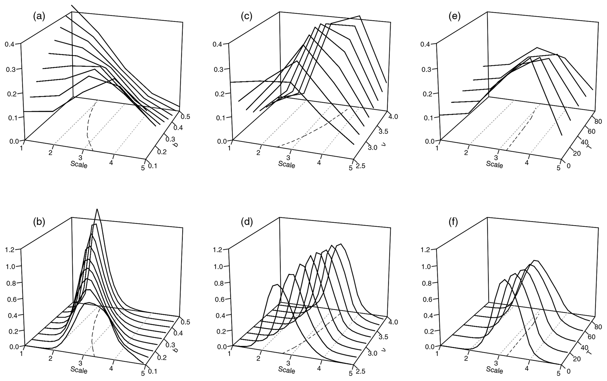
Figure 4 Mean spectra (a, c, e) and histograms of central scale (b, d, f), as functions of the scale parameter b at ν=2.5 (a, b), smoothness parameter ν at b=0.25 (c, d), and threshold T at b=0.1 and ν=2.5 (e, f). Dashed lines in the x–y-plane indicate the respective curve centres of mass; dotted grey lines (parallel to the y axis) were added for orientation.

Figure 4a shows the spatial mean spectra, averaged over all directions and realizations, as a function of the scale parameter b (on the y axis). As expected, an increase in b monotonically shifts the centre of these spectra towards smaller scales. Considering the experiment with variable ν (panel c), we find that an increase in smoothness results in a shift towards larger scales. This is in good agreement with the visual impression we get from the example realizations in Fig. 1. The corresponding scale histograms are shown in Fig. 4b and d. We observe that their centres, corresponding to the expectation values of the central scales, are shifted in the same directions (and to a similar extent) as the mean spectra.

In addition to the shift along the scale axis, we observe that the two model parameters have a secondary effect on the shapes of the curves: a decrease in b or ν goes along with flatter mean spectra – the energy is more evenly spread across scales. The histograms react similarly to b, larger scales coinciding with greater variance, while changes in ν have only a minor impact on the histogram's shape.

The final variable model parameter considered here is the threshold T, for which the expected reactions of our wavelet characteristics are less clear: are fields with a larger fraction of precipitating area perceived to be scaled larger or smaller? To investigate this, we set b=0.1 and ν=2.5 and vary the rain area between 10 % and 100 %. Figure 4e and f shows that the centres of the spectra and histograms hardly depend on T at all. The spread slightly increases with the threshold in both cases, but the changes are far more subtle than for the other two parameters.

In summary, we note that the two structural parameters ν and b have clearly visible effects on the mean spectra as well as the scale histograms. Metrics that compare the complete curves (as opposed to their centres alone) should be able to distinguish between errors in scale and smoothness since these characteristics have different effects on their location and spread. The effect of the threshold T is only moderate in comparison, but could potentially compensate errors in the other two parameters, which may occasionally lead to counterintuitive results.

6 Wavelet-based scores

Motivated by the previous section's results, we now introduce several possible scores, comparing the spectra and histograms of forecast and observed rain fields. Here, we consider the case of a single deterministic prediction, as well as ensemble forecasts.

6.1 Deterministic setting

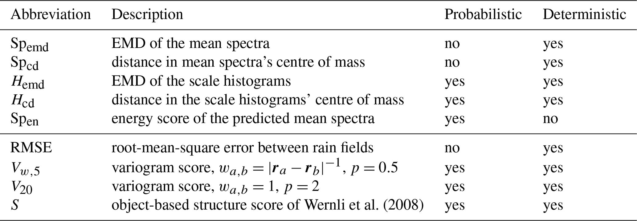
From an observed field and a single deterministic forecast, we obtain the respective mean wavelet spectra and histograms of central scales as described above. If we naively compare these vectors in an element-wise way, we may fall victim to a new incarnation of the double-penalty problem since a small shift in one of the spectra (or histograms) will indeed be punished twice. Rubner et al. (2000) discuss this issue in great detail and suggest the earth mover's distance (henceforth EMD) as an alternative. The EMD between two non-negative vectors (histograms or spectra in our case) is calculated by numerically minimizing the cost of transforming one vector into the other, i.e. moving the dirt from one arrangement of piles to another while doing the minimal amount of work. Here, the locations of the piles corresponding to the histograms (spectra) are given by the centres of the bins (the scales of the spectrum), and the count (energy) determines the mass of the pile. For the simple one-dimensional case where the piles are regularly spaced, the EMD simplifies to the mean absolute difference between the two cumulative histograms (spectra) (Villani, 2003). This quantity is a true metric if the two vectors have the same norm, which is trivially true for the histograms. To achieve the same for the mean spectra, we normalize them to unit sum, thereby removing any bias in total intensity and concentrating solely on structure. Our first two deterministic wavelet-based structure scores are thus given by the EMD between the histograms of central scales (henceforth H_emd) and the normalized, spatially and directionally averaged, wavelet spectra (henceforth Sp_emd), respectively.

Being a metric, the EMD is positive and semi-definite and therefore yields no information on the direction of the error. We can obtain such a judgement by calculating, instead of the EMD, the difference between the respective centres of mass. For the histograms, this corresponds to the difference in expectation value. Rubner et al. (2000) have proven that the absolute value of this quantity is a lower bound of the EMD. Its sign indicates the direction in which the forecast spectrum or histogram is shifted, compared to the observations. We have thus obtained two additional scores, H_cd and Sp_cd, which are conceptually and computationally simpler than the EMD versions and allow us to decide whether the scales of the forecast fields are too large or too small.

6.2 Probabilistic setting

When predictions are made in the form of probability distributions (or samples from such a distribution), verification is typically performed using proper scoring rules (Gneiting and Raftery, 2007). Here, we treat scoring rules as cost functions to be minimized, meaning that low values indicate good forecasts. A function 𝒮 that maps a probabilistic forecast and an observed event to the extended real line is then called a proper score when the predictive distribution F minimizes the expected value of 𝒮 as long as the observations are drawn from F. In this case, there is no incentive to predict anything other than one's best knowledge of the truth. 𝒮 is called strictly proper when F is the only forecast which attains that minimum. As mentioned above, Kapp et al. (2018) verified the spatial mean wavelet spectra via the logarithmic score, which necessitates a further dimension reduction step. In the interest of simplicity as well as consistency with our other scores, we employ the energy score (Gneiting and Raftery, 2007) instead, which is given by

$$\begin{array}{}\text{(4)}& {\displaystyle }\text{En}(F,\mathit{y})=E_F|\mathit{X}-\mathit{y}|-\mathrm{0.5}{E}_F|\mathit{X}-{\mathit{X}}^{\mathbf{\prime }}|,\end{array}$$

where y is the observed vector, E_F denotes the expectation value under the multivariate distribution of the forecast F, and X and X^′ are independent random vectors with distribution F. Here, we substitute the observed mean spectrum for y and estimate F from the ensemble of predicted spectra. The resulting score, which we will denote as Sp_en, is proper in the sense that forecasters are encouraged to quote their true beliefs about the distribution of the spatial mean spectra.

The two previously introduced scores based on the histograms of central scales can directly be applied to the case of ensemble verification by estimating the forecast histogram from all ensemble members pooled together. In this setting where two distributions are compared directly, proper divergences (Thorarinsdottir et al., 2013) take the place of proper scores: a divergence, mapping predicted and observed distributions F and G to the real line, is called proper when its expected minimum lies at F=G. The square of H_cd corresponds to the mean value divergence, which is proper. H_emd is a special case of the Wasserstein distance, the propriety of which is only guaranteed in the limit of infinite sample sizes (Thorarinsdottir et al., 2013). Whether or not these divergences are useful verification tools in the probabilistic case will be tested empirically in Sect. 7.

All of our newly proposed wavelet-based texture scores are listed in Table 1.

Wernli et al. (2008)

Table 1 Wavelet-based structure scores (top part) and established alternatives (bottom).

6.3 Established alternatives

In order to benchmark the performance of our new scores, we compare them to potential non-wavelet alternatives from the literature. A first natural choice is the variogram score of Scheuerer and Hamill (2015), which is given by

$$\begin{array}{}\text{(5)}& {\displaystyle }V(F,\mathit{y})=\sum _{a,b=\mathrm{1}}^n{w}_{a,b}{\left(|y_a-y_b{|}^p-E_F[|X_a-X_b{|}^p]\right)}^{\mathrm{2}},\end{array}$$

where y, F, and X now correspond to the observed rain field, the distribution of the predicted rain fields, and a random field distributed according to the latter. a and b denote two grid points within the domain. The weights w_a,b can be used to change the emphasis on pairs with small or large distances, while the exponent p governs the relative importance of single, extremely large differences. We include two versions of this score in our verification experiment: the naive choice $w_{a,b}=\mathrm{1}$, p=2 (denoted V₂₀ below) and the more robust configuration $w_{a,b}=|{\mathit{r}}_a-{\mathit{r}}_b{|}^{-\mathrm{1}}$, p=0.5 (V_w,5 below), where r_a denotes the spatial location corresponding to the index a. Assuming stationarity of the data, we can efficiently calculate both of these scores by first aggregating the pairwise differences over all pairs with the same distance in space up to a pre-selected maximum distance. V₂₀ then simplifies to the mean-square error between the two stationary variograms. The maximum distance is set to 20, which is a rough approximation of the range of the typical variograms of our test cases. Preliminary experiments have shown that this aggregation greatly improves the performances of V_w,5 and V₂₀ in all of our experiments. It furthermore allows us to apply these scores to the case of deterministic forecasts.

As a second alternative verification tool, we include the S component of the well-known SAL (Wernli et al., 2008). This object-based structure score (1) identifies continuous rain objects in the observed and predicted rain field, (2) calculates the ratio between maximum and total precipitation in each object, (3) calculates averages over these ratios (weighted by the total precipitation of each object), and (4) compares these weighted averages of forecast and observation. The sign of S is chosen such that S>0 indicates forecasts which are scaled too large and/or too flat. In this study, we employ the original object identification algorithm by Wernli et al. (2008), setting the threshold to the maximum observed value divided by 15. We have checked that the sensitivity to this parameter is low in our test cases. For the purposes of ensemble verification, we employ a recently developed ensemble generalization of SAL (Radanovics et al., 2018). Here, the ratio between maximum and total predicted rain is averaged not only over rain objects, but also over the ensemble members.

Lastly, the naive root-mean-square error (RMSE) will be included in our deterministic verification experiment in order to confirm the necessity for more sophisticated methods of analysis.

7 Idealized verification experiments

For our first set of randomly drawn forecasts and observations from the model given by Eq. (1), we keep the threshold T constant such that 20 % of the fields have non-zero values and select four combinations of ν and b, listed in Table 2.

Table 2 Varying parameters in Eq. (2) for the four groups of artificial ensemble forecasts.

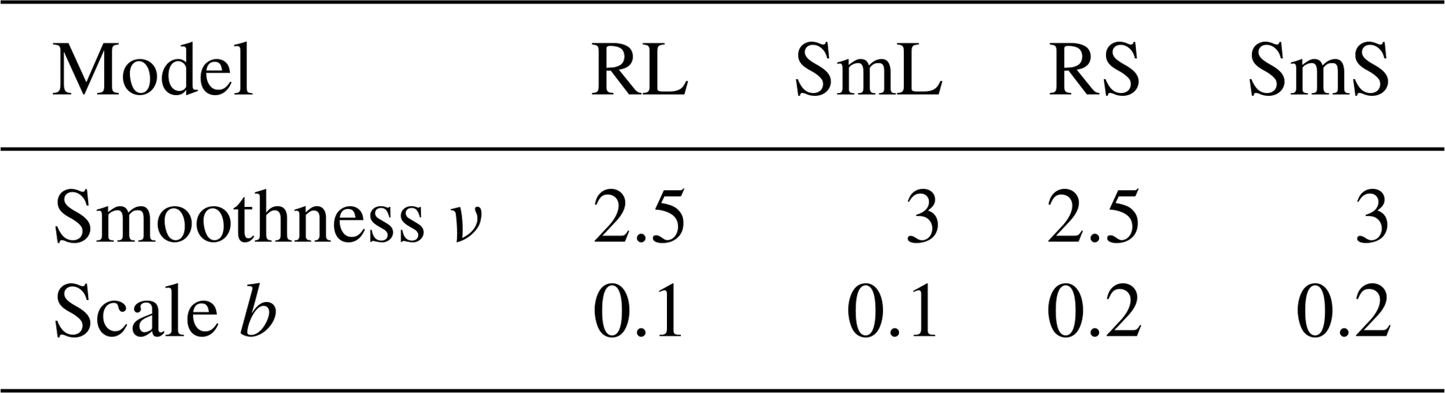
The resulting texture is rough and large scaled (RL), smooth and large scaled (SmL), rough and small scaled (RS), and smooth small scaled (SmS). One realization for each of those settings is depicted in Fig. 1. In the following sections, we interpret random samples of these models as observations and forecasts, thus allowing us to observe how frequently the truly best prediction (the one with the same parameters as the observation) is awarded the best score.

7.1 Ensemble setting

Beginning with the synthetic ensemble verification experiment, we draw 100 realizations each from RL and RS as our observations. For every observation (200 in total), we issue four ensemble predictions, consisting of 10 realizations from RL, SmL, RS, and SmS, respectively. Only one of these 10-member ensembles thus represents the correct correlation structure while the other three are wrong in either scale, smoothness, or both. Observation and ensembles are compared via the three wavelet scores H_cd, H_emd, and Sp_en as well as the established alternatives for ensemble forecasts, i.e. S, V₂₀, and V_w,5.

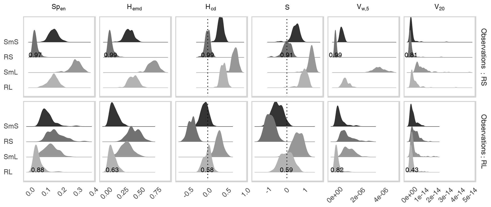
Figure 5 Distribution of all probabilistic scores for each of the forecast ensembles corresponding to the four models from Table 2. Top row: observations drawn from RS. Bottom row: observations drawn from RL. Numbers denote the fraction of cases in which the forecast from the correct distribution received the best score.

Figure 5 shows the resulting score distributions. All scores are best when small, except for the two-sided S and H_cd where values near zero are optimal. Beginning with the case where the observations are drawn from RS (top row of Fig. 5), we observe that the four predictions are ranked quite similarly by all scores. Here, the correct forecast almost always receives the best mark, while SmL, which is most dissimilar from RS, fares worst. S and H_cd furthermore agree that all three false predictions are scaled too large. The task of determining the truly best forecast is substantially more complicated when the observations belong to RL (bottom row of Fig. 5): since SmS is both smoother and scaled smaller, the effects on the location of the spectra and histograms along the scale axis (cf. Fig. 4) compensate each other. These curves can therefore hardly be distinguished by their centres of mass alone. We recognize that RL and SmS consequently obtain similar values of H_cd, this score judging solely based on the centres. The other two wavelet scores achieve better discrimination, as does V_w,5. Concerning the signs of the error, we note that S and H_cd both consider RS too small and SmL too large. For SmS, H_cd is only slightly negative, indicating nearly correct scales. S is less affected by the compensating effect of increased smoothness and determines more clearly that SmS is smaller-scaled than RL. Its overall success rate is, however, not significantly better than that of H_cd.

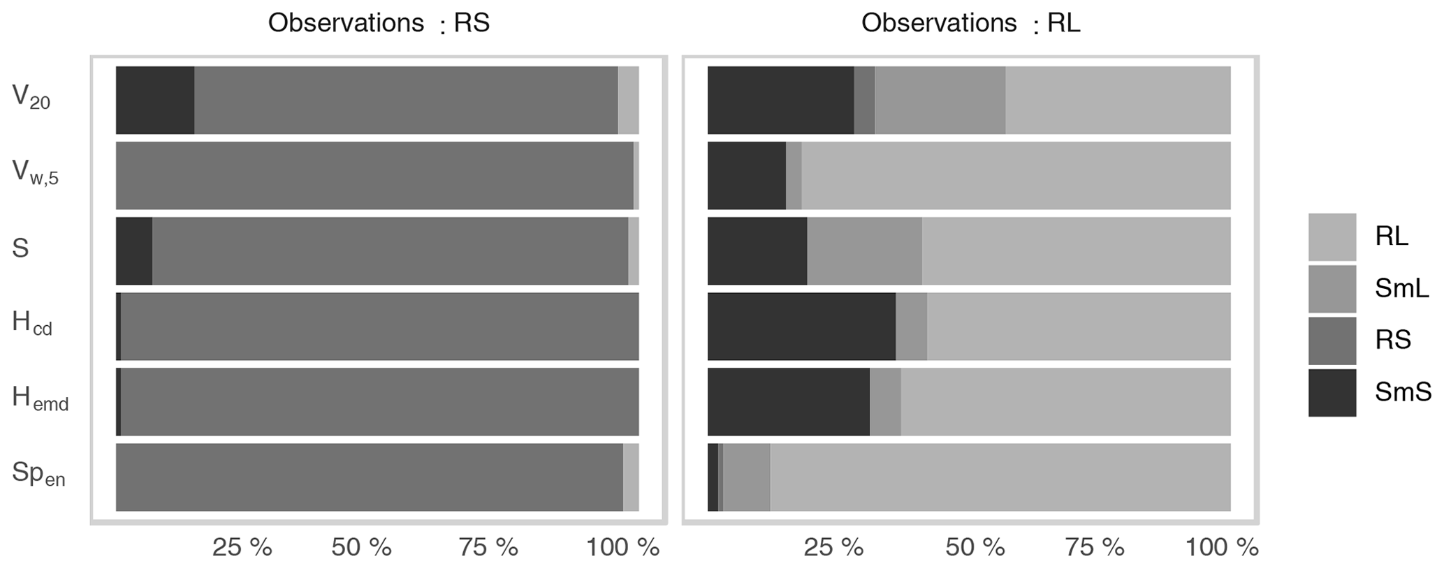
Figure 6 Percentage of cases where each of the four ensembles corresponding to the models in Table 2 was deemed the best forecast, separated by score and the model of the observation.

Figure 6 summarizes the ability of the six tested probabilistic scores to correctly determine the best forecast ensemble. As discussed above, all scores are very successful at determining correct forecasts of RS. In the alternative setting (observations from RL), SmS is the most frequent wrong answer, receiving the smallest (absolute) values of V₂₀, S, H_cd, and H_emd in more than a quarter of cases. In contrast to the other scores, Sp_en hardly ever erroneously prefers SmS over RL. Instead, SmL is wrongly selected most frequently, leading to the overall lowest error rate (12 %) in this part of the experiment.

7.2 Deterministic setting

Having investigated the behaviour of our probabilistic scores, we now consider the deterministic case: how successfully can we determine the truly best forecast, given only a single realization? The set-up for this experiment is the same as before, only the size of the forecast ensembles is reduced from 10 to 1. Since the resulting scores naturally have greater variances than before, we increase the number of observations to 1000 (500 each from RL and RS) in order to achieve similarly robust results. In addition to the four appropriate wavelet scores (Sp_emd, Sp_cd, H_emd and H_cd), we again calculate V_w,5 and V₂₀ as well as the S component of the original SAL score. To ensure that the verification problem is sufficiently difficult, the root-mean-square error (RMSE) is included as a naive alternative as well.

Figure 7 As Fig. 6, but for the deterministic verification experiment.

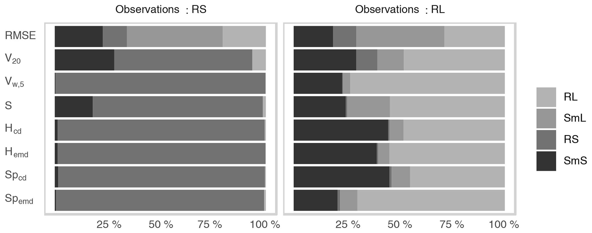
Figure 7 reveals that correct forecasts are again easily identified by all of the wavelet-based scores when the observed fields belong to RS. As in the ensemble scenario, the main difficulty lies in the decision between SmS and RL in cases where the latter model generates the observations. The two EMD scores, which use the complete curves and not just their centres, clearly outperform the corresponding CD versions in this part of the experiment and detect RL correctly in the majority of cases. V_w,5 is similarly successful as the best wavelet-based score, faring marginally better than Sp_emd. The failure rates of V₂₀ and S are again slightly higher. Unsurprisingly, the RMSE is completely unsuited to the task at hand, achieving less than 25 % correct verdicts overall. The inferiority to a random evaluation, which would, on average, be correct one-fourth of the time, is caused by the fact that the model with the largest, smoothest features (SmL) has the least potential for double penalties and thus fares best in a point-wise comparison; in fact, RMSE orders the four models by their typical features size, irrespective of the distribution of the observation.

7.3 Wavelet choice and bias correction

One obvious question to ask is whether or not the choice of the mother wavelet has a significant impact on the success rates in the two experiments discussed above. To address this issue, we repeat both the deterministic and the ensemble verification processes for several Daubechies wavelets. Recalling the results of our objective wavelet selection (Sect. 3 and Appendix A), we expect no dramatic effects.

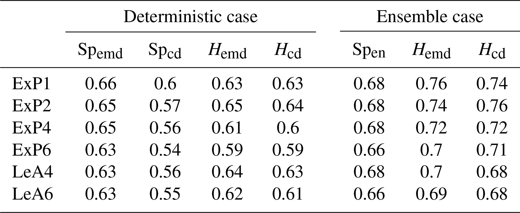
Table 3 Fraction of cases where the correct forecast received the best score for a range of extremal phase (ExP) and least asymmetric (LeA) Daubechies wavelets. LeA4 is the wavelet used for all other experiments in this study; ExP1 is the well-known Haar wavelet.

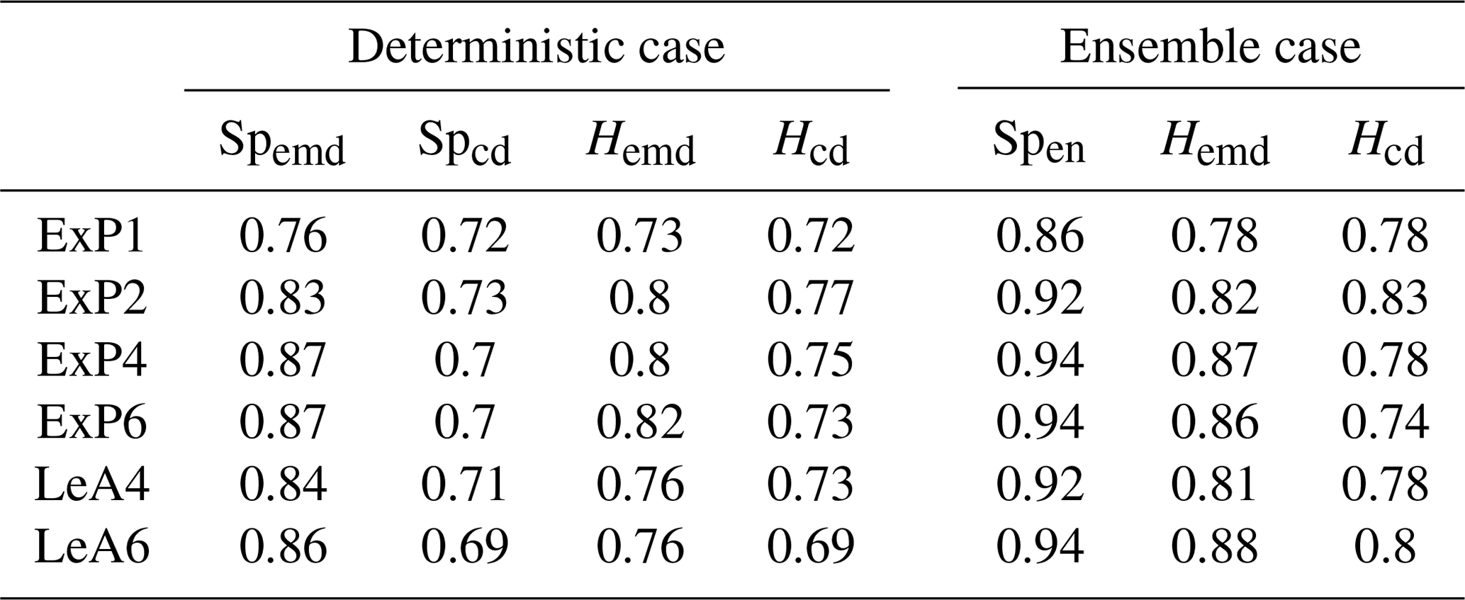
Table 3, listing the overall success rates for each tested wavelet, mostly confirms this expectation: in the deterministic case, Sp_emd and H_emd are really only affected by the choice between the Haar wavelet, which performs worst, and any of its smoother cousins. The two centre-based scores (Sp_cd and H_cd) show hardly any wavelet dependence at all. Sensitivities are overall slightly higher in the ensemble case. While D₁ again appears to be the worst choice, there are some differences between the other options, particularly for the two histogram scores. Generally speaking, the impacts of wavelet choice on our verification results are nonetheless rather limited, as long as the Haar wavelet is avoided.

Table 4 As Table 3, but without the bias-correction step.

To confirm that the bias correction following Eckley et al. (2010) is indeed a necessary part of our methodology, we repeat these experiments without applying the correction matrix A⁻¹. Without discussing the details (Table 4), we merely note that the success rates decrease substantially (depending on score and wavelet), meaning that bias correction generally cannot be skipped.

7.4 Perturbed thresholds

Next, we consider the case where forecast and observations are subject to random perturbations which are not directly related to the underlying covariance model. One rather natural way of implementing this scenario consists of randomly perturbing the thresholds, i.e. the fractions of the domain covered by non-zero precipitation. In a realistic context, such random differences between forecast and observation could be associated with a displacement error which shifts unduly large or small parts of a precipitation field into the forecast domain.

Table 5 Fraction of cases where the correct forecast received the best score. Top two rows: deterministic forecasts with and without perturbed threshold. Bottom: ensemble forecasts with and without perturbed thresholds.

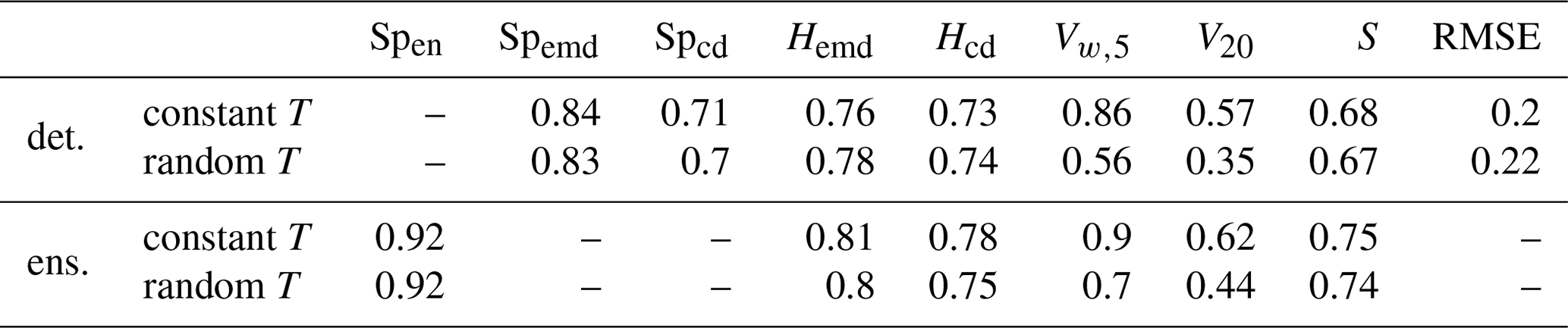
Our experiments in Sect. 5 indicate that the wavelet-based scores should be relatively robust to small changes in the threshold T (cf. Fig. 4e and f). For the variogram scores, one might expect greater sensitivity since the presence of a fixed fraction of zero values greatly reduces the variance in the pairwise distances from which the stationary variogram is estimated. To test these hypotheses, we again repeat the two verification experiments, this time randomly varying T such that the precipitation area, previously fixed at 20 %, is a uniform random variable between 15 % and 25 % of complete domain.

Looking at the resulting success rates (Table 5), we find our expectations largely confirmed: while variations in the precipitation coverage hardly influence our wavelet-based judgement, V_w,5 and V₂₀ seem to strongly depend on this parameter, thus mostly losing their ability to determine the correct model. The performances of S and RMSE are only weakly influenced by variations in T.

8 Summary and discussion

The basic idea of this study is that the structure of precipitation fields can be isolated and subsequently compared using two-dimensional wavelet transforms. Building on the work of Eckley et al. (2010) and Kapp et al. (2018), we have argued that the corrected, smoothed version of the redundant discrete wavelet transform (RDWT) is an appropriate tool for this task since it is shift invariant and has a proven asymptotic connection with the correlation function of the underlying spatial process. This approach is theoretically more flexible than Fourier- or variogram-based methods which make some form of global stationarity assumption, while our method relies on the substantially weaker requirement of local stationarity.

Before wavelet-transformed forecasts and observations can be compared to one another, the spatial data must be aggregated in a way that avoids penalizing displacement errors twice. Besides the proven strategy (Kapp et al., 2018) of averaging the wavelet spectra over all locations, we have newly introduced the map of central scales as a potentially interesting alternative: by calculating the centre of mass for each local spectrum, we obtain a matrix of the same dimensions as the original field, each value quantifying the locally dominant scale. Aside from the possibility of compactly visualizing the output of the RDWT in a single image, the histogram of these scales can serve as an alternative basis for verification, emphasizing each scale based on the area in which it dominates, rather than the fraction of total rain intensity it represents.

In order to rigorously test the sensitivity of these aggregated wavelet transforms to changes in the structure of rain fields, a controlled but realistic test bed was needed. The stochastic precipitation model of Hewer (2018) constitutes a very convenient case study for our purposes: the construction based on the moisture budget and a Helmholtz-decomposed wind field allows for non-Gaussian behaviour and guarantees that the simulated data are more realistic than simple geometric patterns or Gaussian random fields. The model's structural properties can nonetheless be determined at will via the smoothness and scale parameter of the underlying Matérn fields, allowing us to simulate observations and forecasts with known error characteristics. In a realistic context, errors in scale correspond to misrepresentation of feature sizes (e.g. smoother representation of small-scale convective organization), while errors in smoothness correspond to forecast models with a resolution that is too course, which are incapable of reproducing fine structures.

In a first suite of experiments we found that the wavelet spectra do indeed react sensitively to changes in both of these parameters. In particular, errors in smoothness and scale have different signatures which can potentially be differentiated from one another. Encouraged by these results, we have defined several possible scores which compare mean spectra and scale histograms via the difference between their centres (H_cd and Sp_cd), their earth mover's distance (H_emd and Sp_emd), and the energy score (Sp_en). In our idealized verification experiments, the performance of the latter three scores, i.e. their ability to correctly determine the objectively best forecast, was on par with the best tested variogram score (V_w,5). The less robust V₂₀, as well as the SAL's structure component S and the simplistic RMSE, was clearly outperformed. H_cd and Sp_cd, while less proficient at finding the correct answer, do yield valuable auxiliary information in the form of the error's sign, answering the question of whether the predicted structure was too coarse or too fine. Keeping in mind that both spectra and histograms can have multi-modal structures in realistic non-stationary cases (compare Fig. 3d), a comparison based on centres alone is likely not sufficient and the EMD versions of these scores should be preferred. If a signed structure score is desired, we can simply multiply the respective EMD by the sign of the difference in centres.

All five wavelet scores were shown to be robust to small perturbations of the data, realized here as random changes to the fraction of non-zero rain. In these experiments, which essentially test the score's sensitivity to the sample climatology, the variograms largely lost their ability to determine the correct forecast. Interpreting this result, it is important to keep in mind that our wavelet scores were specifically designed to judge based on structure alone while the variogram-methodology of Scheuerer and Hamill (2015) allows for a more holistic assessment. Sensitivity to precipitation coverage is therefore not necessarily a disadvantage. If the goal is a pure assessment of structure, this dependence is undesirable.

The two free parameters of the variogram score, namely the exponent p and the choice of weights w_i,j, were found to have a significant impact on the resulting verification. We have also tested the sensitivity of the newly introduced wavelet scores to the choice of the mother wavelet. An objective wavelet-selection procedure following Goel and Vidakovic (1995) was performed and the verification experiments were repeated for a variety of possible choices. Summarizing both of these steps, we can conclude that the success of our wavelet-based verification depends only weakly on the choice of an appropriate mother wavelet. One somewhat surprising exception is the Haar wavelet, which was favoured by previous studies (cf. Weniger et al., 2017, and references therein) but turned out to be a suboptimal choice for our purposes.

Now that the merits of wavelet-based structure scores have been demonstrated in a controlled environment, further tests are needed to study their behaviour in real-world verification situations. One important open question concerns the use of direction information, which was neglected in the present study but may well be valuable in a more realistic scenario. It is furthermore worth noting that, in contrast to primarily rain-specific tools like SAL, our methodology can be applied to any variable of interest with no major changes besides the new selection of an appropriate mother wavelet. A simultaneous evaluation of, for example, wind components, humidity, and cloud-cover – using the exact same verification tool to assess structural agreement in each variable – is thus feasible and could answer interesting questions concerning the origins of specific systematic forecast deficiencies.

Appendix A: Entropy-based wavelet selection

To find the most appropriate wavelet, we calculate the entropy of the transform's squared coefficients (representing the energy of the transformed data) and select the wavelet with the smallest entropy. Let $\mathit{y}=(y_{\mathrm{1}},\mathrm{\dots },y_n{)}^T$ be a vector with non-negative entries satisfying ${\sum }_i{y}_i=\mathrm{1}$. For our purposes, its entropy is defined as

$$\begin{array}{}\text{(A1)}& {\displaystyle }s\left(\mathit{y}\right):=-\sum _{i=\mathrm{1}}^n{y}_i{\log }_{\mathrm{2}}{y}_i\in [\mathrm{0},{\log }_{\mathrm{2}}(n\left)\right],\end{array}$$

where we set $\mathrm{0}\cdot {\log }_{\mathrm{2}}\left(\mathrm{0}\right)=\mathrm{0}$. Following Goel and Vidakovic (1995), the RDWT is replaced by its corresponding orthogonal decomposition, which is obtained by selecting every second of the finest-scale coefficients, every fourth on the second-finest scale, and so on. The number of data points is thus conserved under the transformation and we can compare the entropy of the transformed data to that of the original representation.

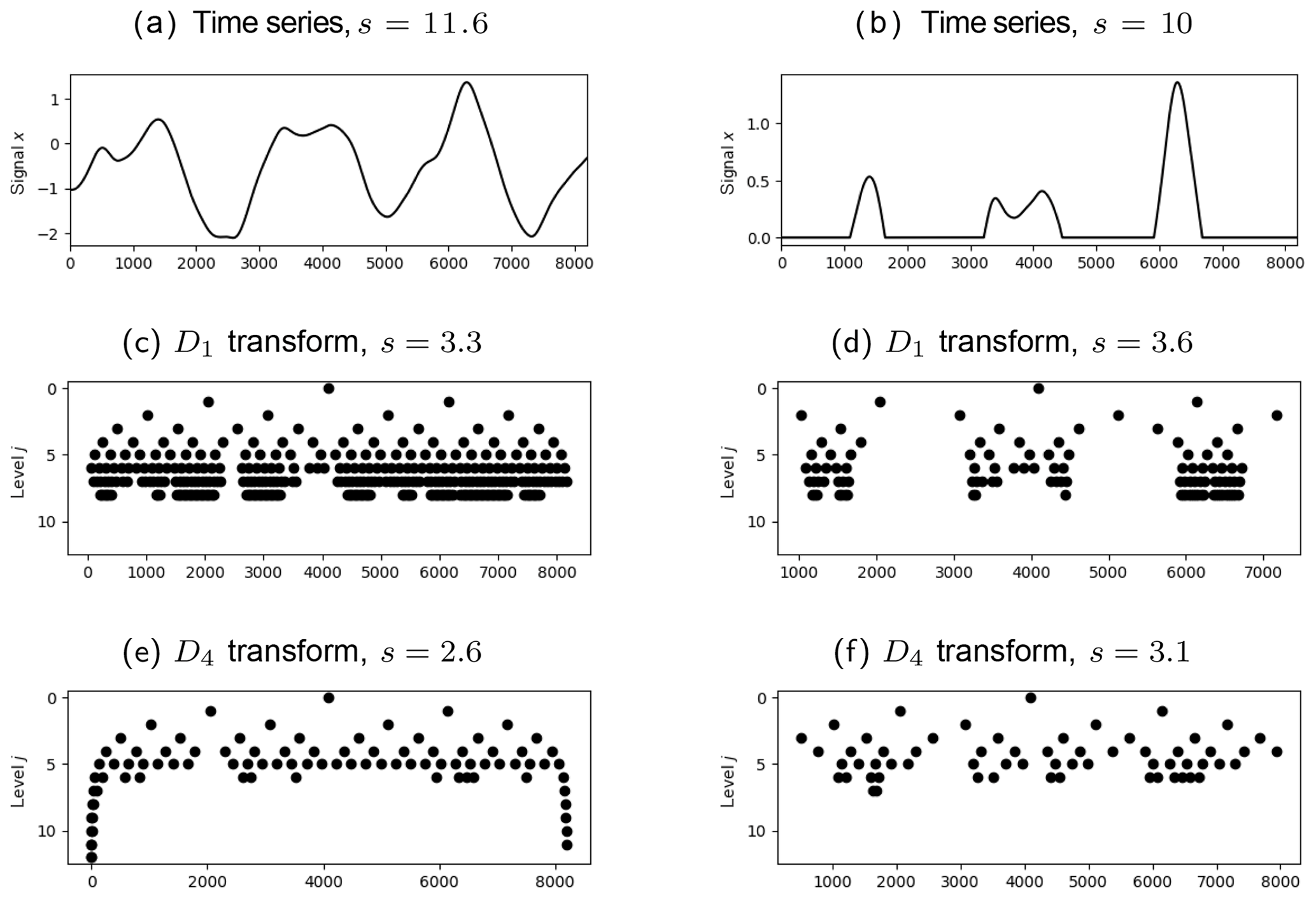
Figure A1 Realization of a one-dimensional Gaussian random vector with covariance $M(\mathit{\nu }=\mathrm{3.5},b=\mathrm{2})$ (a) and the corresponding values of the D₁ transform and least asymmetric D₄ transform (c, e) which are greater than 0.1. Panels (b), (d), and (f) are the corresponding plots for the cases where the vector is cut off at zero.

The outcome of this procedure depends on the structure of the data to be transformed, the smoothness of the wavelet, and the length of its support. To understand how these properties interact, we quantify smoothness via the number of vanishing moments: a wavelet ψ is said to have N vanishing moments if $\int x^q\mathit{\psi }\left(x\right)\mathrm{d}x=\mathrm{0}$ for $q=\mathrm{0},\mathrm{\dots },N-\mathrm{1}$. This implies that polynomials of order N−1 have a very sparse representation in the wavelet basis corresponding to ψ. The theorem of Deny-Lions (Cohen, 2003) relates this property to a function's differentiability: loosely speaking, if f is N times differentiable, the error made when approximating f by polynomials of order N−1 is bounded by a constant times the energy of f's Nth derivative f^(N). It follows that f is well represented by wavelets with N vanishing moments, as long as f^(N) is not too large.

Besides more or less smooth regions within the rain fields (in our test cases governed by the parameter ν) and constant zero areas outside, the data we wish to transform also contain singularities at the edges of precipitating features. Here, f^(N) is generally not small and wavelets with shorter support length are superior since fewer coefficients are affected by any given singularity. Heisenberg's uncertainty principle ensures that localization in space and approximation of polynomials (related to the localization in frequency) cannot both be optimal simultaneously: if a wavelet has N vanishing moments, then its support size (in one dimension) is at least 2N−1. In proving this theorem, Daubechies (1988) introduced the D_N wavelets, which are optimal in the sense that they have N vanishing moments at the smallest possible support.

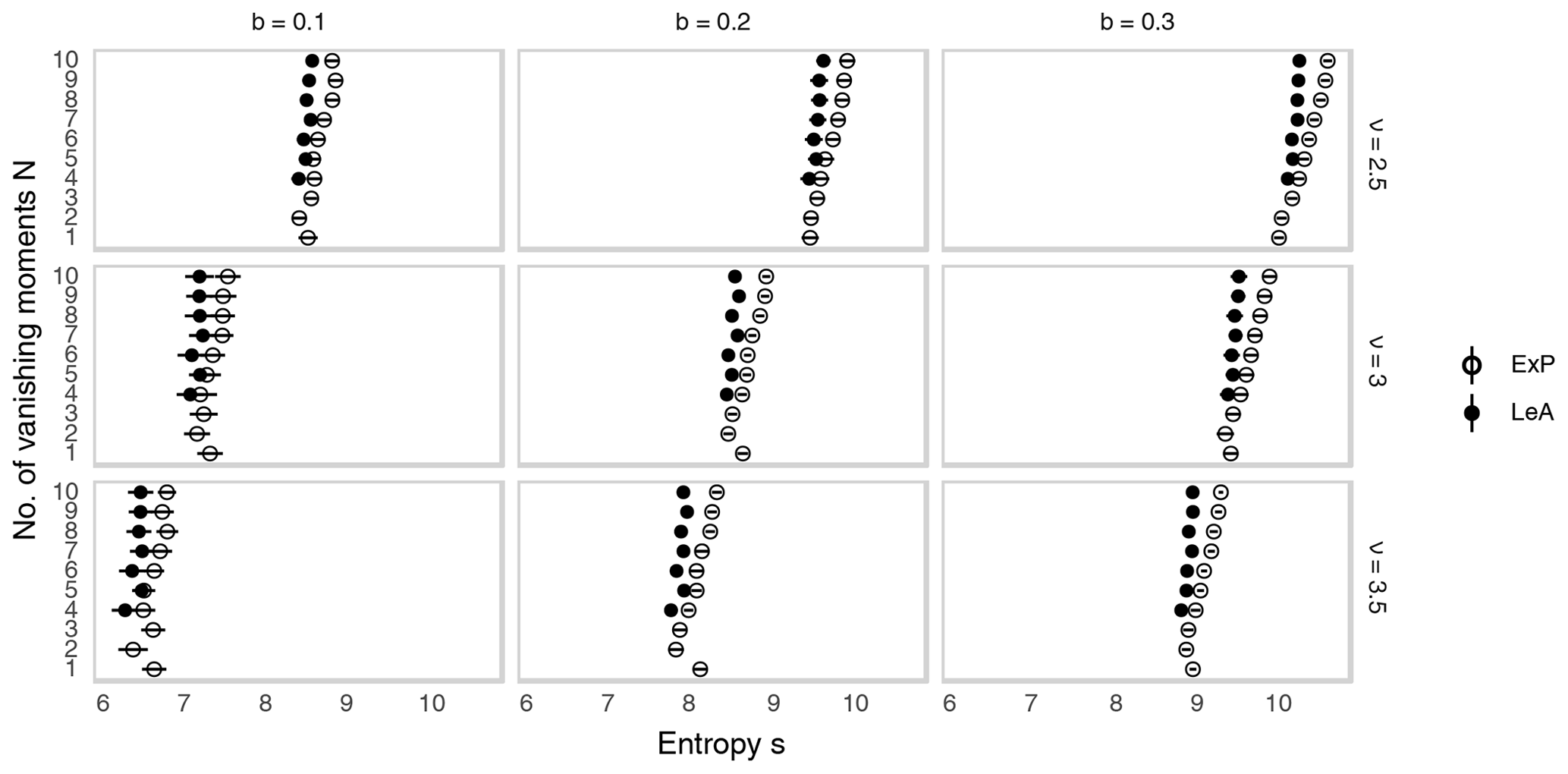
Figure A2 Entropy of the wavelet-transformed synthetic rain fields from Fig. 1 as a function of the wavelet's order N. Empty and filled dots correspond to the extremal phase version and least asymmetric version of D_N, respectively. Lines indicate 1 standard deviation, estimated from 10 realizations.

To illustrate the competing effects of support size and smoothness on the efficiency of the wavelet transformation, we simulate one-dimensional Gaussian random fields with Matérn covariances (same function M and parameters b and ν as in Eq. 2, but only one variable and one spatial dimension). Figure A1 neatly demonstrates the concepts discussed above: when the time series is uniformly smooth, the higher order wavelet D₄ delivers a far more efficient compression than D₁ (panels a, c, e). The situation changes when we truncate the data (b, d, f): while D₄ continues to be superior within the smooth regions, D₁, due to its shorter support, requires fewer coefficients to represent the regions of constant zero values. This trade-off between representing smooth internal structure and intermittency is precisely quantified by the entropy (defined in Eq. A1, values noted in the captions of Fig. A1), which measures the total degree of concentration on a small number of coefficients: while the D₄ does better in both cases, the relative and absolute improvement is worse in the cut off case, where we introduced artificial singularities.

Figure A2 shows the results of our entropy-based wavelet-selection procedure for the model given by Eq. (1). We observe that the model parameters have substantially more impact on the efficiency of the compression than the choice of wavelet. Fields with greater smoothness and larger scales (large values of ν and small values of b) are represented far more compactly than rough small-scale cases, irrespective of the chosen basis. The differences between wavelets, while small in comparison, reveal a systematic behaviour: increasing support length leads to monotonously worse compression and the least asymmetric wavelets tend to fit slightly better than their “extremal phase” counterparts. The Haar wavelet constitutes an exception to this pattern, its entropy being frequently larger than that of several of its smoother cousins.

Figure A3 Ratio of negative to positive energy in the mean spectra (data set from Sect. 7.3, all models from Table 2, six selected mother wavelets as in Table 3).

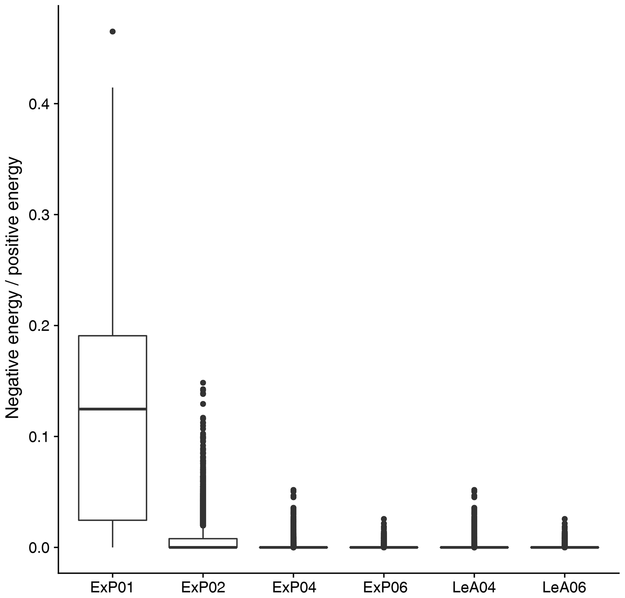
Besides theoretical optimality motivated by Eq. (3), practical concerns can play an important role in the selection of an appropriate wavelet as well. Recalling that the bias-correction following Eckley et al. (2010) can introduce negative values to the spectra, which have no intuitive interpretation, we are interested in seeing whether the problem can be circumvented by selecting an appropriate mother wavelet. Fig. A3 shows the ratio between negative and positive energy in the mean spectra from the experiments discussed in Sect. 7.3. For D₁, this ratio is typically close to one-tenth. Such large quantities of negative energy are rare for D₂ and basically never occur in higher-order wavelets. This observation, while reassuring, does not alter our wavelet selection since the Haar wavelet was not favoured by the entropy-based approach either.