the Creative Commons Attribution 4.0 License.
the Creative Commons Attribution 4.0 License.
 | 26 Jul 2019
PatCC1: an efficient parallel triangulation algorithm for spherical and planar grids with commonality and parallel consistency
Haoyu Yang
Li Liu
Cheng Zhang
Ruizhe Li
Chao Sun
Xinzhu Yu
Zhiyuan Zhang
Bin Wang
Graphs are commonly gridded by triangulation, i.e., the generation of a set of triangles for the points of the graph. This technique can also be used in a coupler to improve the commonality of data interpolation between different horizontal model grids. This paper proposes a new parallel triangulation algorithm, PatCC1 (PArallel Triangulation algorithm with Commonality and parallel Consistency, version 1), for spherical and planar grids. Experimental evaluation results demonstrate the efficient parallelization of PatCC1 using a hybrid of MPI (message passing interface) and OpenMP (Open Multi-Processing). They also show PatCC1 to have greater commonality than existing parallel triangulation algorithms (i.e., it is capable of handling more types of model grids) and that it guarantees parallel consistency (i.e., it achieves exactly the same triangulation result under different parallel settings).
- Article
(4136 KB) - Full-text XML
-
Supplement
(173 KB) - BibTeX
- EndNote


A coupler is a fundamental component or library used in models for Earth system modeling. It handles coupling between component models or even between the internal processes or packages of a component model. A coupler's fundamental functions are data transfer (between different component models, processes, or packages) and data interpolation (between different model grids) (Valcke et al., 2012) that can refer to horizontal remapping, vertical remapping, grid staggering, and vector interpolation for various types of coupling fields. Most existing couplers have the capability of horizontal remapping of coupling fields between different horizontal grids, especially spherical grids. As the horizontal grids of models generally remain unchanged throughout the time integration of a simulation, the data interpolation function of a coupler is generally divided into two stages: the first calculates the remapping weights for a source horizontal grid to a target horizontal grid, and the second uses the same remapping weights to calculate the remapping results at each instance of data interpolation. Most existing couplers can read in offline remapping weight generated by other software tools such as SCRIP (Jones, 1999), ESMF (Hill et al., 2004), and YAC (Hanke et al., 2016), while some couplers such as OASIS (Redler et al., 2010; Valcke, 2013; Craig et al., 2017) and C-Coupler (Liu et al., 2014, 2018) also have the ability of generating online remapping weights. Online remapping weights generation can obviously improve the friendliness of couplers because users will no longer be forced to manually generate offline remapping weights after changing model grids or resolutions.
Commonality can be viewed as a fundamental feature of a coupler. For example, most existing couplers such as OASIS, CPL (Craig et al., 2005, 2012), MCT (Larson et al., 2005), and C-Coupler have been used in a range of coupled models. In the past, the longitude–latitude grid (i.e., a regular grid) was most widely used. However, the rapid development of Earth system modeling has seen various types of new horizontal grids appear, such as the reduced Gaussian grid, tripolar grid, displaced pole grid, cubed-sphere grid, icosahedral grid, Yin–Yang grid, and adaptive mesh, some of which are unstructured. The continuous emergence of new types of horizontal grids introduces a significant challenge to the commonality of couplers, especially the commonality of data interpolation between any two horizontal grids. There are in general two options to address this challenge: either the new types of horizontal grids are incrementally supported via incremental upgrades of the code of a coupler or remapping software as required or a common representation is designed and developed for various types of horizontal grids and then the remapping weights are calculated based on the common grid representation, thus allowing the code of a coupler or remapping software to remain almost unchanged throughout the development of model grids. As the first option will result in the code of a coupler or remapping software to become increasingly complicated, the second option is preferred, provided a common grid representation can be found.
A common grid representation can be achieved by first viewing a grid as a set of independent grid points (only the coordinate values of each point are concerned, while the relationships among grid points – e.g., that one grid point is the neighbor of another – are neglected) and next using one specific gridding method to build relationships among the grid points. Triangulation is a widely used gridding method that generates a set of triangles for independent points in a graph. Therefore, its use can potentially improve the commonality of data interpolation. In fact, triangulation has already been used by couplers, such as C-Coupler.
Existing triangulation algorithms do not have high time complexity. For example, Delaunay triangulation (Su and Drysdale, 1997), which is a widely used triangulation algorithm, has a time complexity of O(NlogN) for N points. However, the overhead of triangulation cannot always be neglected, especially as model grids gain increasing numbers of points as the model resolution increases. Modern high-performance computers equipped with increasing numbers of computing nodes containing increasing numbers of processor cores can dramatically accelerate various applications, including triangulation, that can be efficiently parallelized. MPI (message passing interface) is a widely used parallel programming library that can explore the parallelism of processor cores either in the same computing node or among different nodes, while OpenMP (Open Multi-Processing) is a widely used parallel programming directive that can explore the parallelism of processor cores in the same computing node. For higher parallel efficiency, many applications (including models for Earth system modeling) have benefited from the hybrid use of both MPI and OpenMP, where MPI generally directs the parallelism among computing nodes and OpenMP controls that of processor cores within the same computing node. Some existing couplers, such as MCT, OASIS3-MCT_3.0 (Craig et al., 2017), and C-Coupler2 (Liu et al., 2018), work as libraries and generally share the parallel setting used by a component model. When a component model utilizes a hybrid of both MPI and OpenMP for parallelization, a parallel triangulation algorithm that has been integrated in a coupler will waste the parallelism of processor cores exploited by OpenMP if the triangulation algorithm only utilizes MPI for parallelization.
Existing couplers such as MCT, CPL6/CPL7, OASIS3-MCT_3.0, and C-Coupler2 can achieve parallel consistency, which means achieving exactly the same results under different parallel settings. Parallel consistency is important for debugging parallel implementations. Without it, distinguishing reasonable errors and faults introduced by parallelization is very difficult. However, the parallelization of triangulation algorithms may damage their consistency. To develop efficient parallel triangulation algorithms, the entire grid domain is generally decomposed into a set of subgrid domains, the triangulation on each subgrid domain is conducted independently, and the overall result of triangulation is obtained through merging or stitching the triangles from all subgrid domains. If the merging or stitching does not force parallel consistency, a parallel triangulation algorithm may obtain different triangles under different parallel settings. As a result, a coupler may not be able to guarantee parallel consistency after implementing such a parallel triangulation algorithm.
Therefore, for a triangulation algorithm to be potentially useful in a coupler, it will need to show consistently all three of the following features: commonality (capable of handling almost every type of model grid), parallel efficiency (efficient parallelization with a hybrid of MPI and OpenMP), and parallel consistency. There are several parallel triangulation algorithms that can handle spherical grids (most model grids are spherical grids): for example, the algorithm proposed by Larrea (2011) (called the Larrea algorithm hereafter), the algorithm proposed by Jacobsen et al. (2013) (called the Jacobsen algorithm hereafter), and an improved algorithm based on the Jacobsen algorithm (Prill and Zängl, 2016) (called the Prill algorithm hereafter). However, none of them simultaneously achieve the three required features (Sect. 2). With the aim of achieving these three features, we designed and developed in this work a new parallel triangulation algorithm named PatCC1 (PArallel Triangulation algorithm with Commonality and parallel Consistency, version 1) for spherical and planar grids. Evaluations using various types and resolutions of model grids and different parallel settings reveal that PatCC1 can handle various types of model grids, achieve good parallel efficiency, and guarantee parallel consistency.
The remainder of this paper is organized as follows. We briefly introduce related works in Sect. 2, introduce the overall design of PatCC1 in Sect. 3, describe the implementation of PatCC1 in Sect. 4, evaluate PatCC1 in Sect. 5, and briefly summarize this paper and discuss future work in Sect. 6.
This section further introduces the Larrea, Jacobsen, and Prill algorithms in detail.
The Larrea algorithm aims to triangulate global grids. It first uses a 1-D decomposition approach to decompose a global grid into nonoverlapping subgrid domains of stripes (the boundaries of each subgrid domain are longitudes) and next assigns each subgrid domain to an MPI process (OpenMP is not used in the parallelization) for local triangulation. To obtain the overall result of triangulation, it collects the local triangles generated by each MPI process and stitches them together using an incremental triangulation algorithm (Guibas and Stolfi, 1985), but without guaranteeing parallel consistency. Therefore, the Larrea algorithm has limitations on commonality, parallel efficiency, and parallel consistency.
The Jacobsen algorithm can triangulate spherical and planar grids. It first decomposes the whole grid domain into partially overlapping circular subgrid domains and next instructs each MPI process (OpenMP is not used in the parallelization) to conduct 2-D planar triangulation for a circular subgrid domain, where the points on a spherical grid are projected onto a plane before the triangulation. To obtain the overall result, it first collects together the local triangles generated by each MPI process and next scans each triangle, where a triangle is pruned from the overall result if the same triangle already exists. As this algorithm does not check or guarantee parallel consistency, it introduces a risk of overlapping triangles in the overall result. Although it is aimed for use with spherical grids and planar grids, the evaluation in Sect. 5.2 shows that it is still unable to handle some types of model grids well such as longitude–latitude grids and grids with concave boundaries.
As an upgraded version of the Jacobsen algorithm, the Prill algorithm achieves the following two improvements, but without improving the commonality or the parallel consistency. First, OpenMP is further used in parallelization, which means that parallelization uses a hybrid of MPI and OpenMP. Second, the centers of circular subgrid domains are determined adaptively, while the circle centers in the Jacobsen algorithm must be specified by the user. The Prill algorithm uses a 3-D spherical triangulation implementation rather than a 2-D planar triangulation implementation.
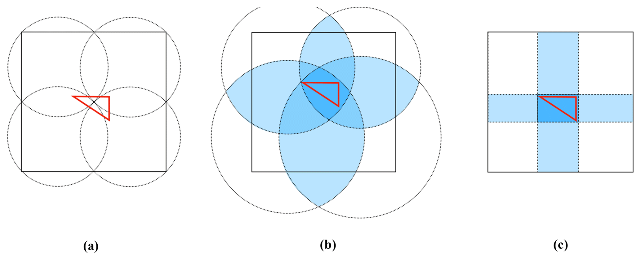
The first step of a parallel triangulation algorithm is to decompose the whole grid domain into subgrid domains. Generally, three questions should be considered in designing a decomposition approach. The first is whether there should be overlapping regions among the subgrid domains. The Larrea algorithm does not have overlapping regions among the subgrid domains, so triangles across the boundaries of subgrid domains are not obtained through the local triangulation for each subgrid domain but are calculated during the last step that obtains the overall triangulation result. We do not prefer such an implementation as it requires the development of a program that can efficiently calculate in parallel the triangles across boundaries. The second consideration is the choice of the general shape of subgrid domains. We prefer rectangles rather than the stripes used in the Larrea algorithm and the circles used in the Jacobsen and the Prill algorithms because the 1-D decomposition corresponding to a petaloid shape will limit the parallelism of a parallel triangulation algorithm, and a circle-based decomposition is disadvantageous in terms of extra overhead. For example, Fig. 1a shows a triangle that should be obtained from the correct triangulation of the whole grid domain that is rectangular and a decomposition of the whole grid domain into four circles. Although these circles are partially overlapping, none of them fully covers the unique triangle in Fig. 1a. To achieve proper triangulation, these circles should be enlarged accordingly, as in Fig. 1b, where each circle fully covers the triangle. Figure 1c shows a decomposition into four rectangles, each of which also fully covers the triangle. As larger regions of overlap generally mean increased overhead for parallelization, the comparison between Fig. 1b and c indicates that a circle-based decomposition will introduce higher extra costs than rectangle-based decomposition. The third question is whether it is reasonable to force uniform areas among the subgrid domains. We prefer to support nonuniform areas because the time complexity as well as the overhead of triangulation is generally determined by the number of grid points, while different subgrid domains with uniform area may have significantly different numbers of points. In summary, PatCC1 should conduct grid domain decomposition using partially overlapping rectangles of nonuniform area.
The next step after decomposing the whole grid is to triangulate each subgrid domain separately. Generally, an existing sequential algorithm can be used for this step. Although a spherical grid is on a surface in 3-D space, we prefer 2-D triangulation algorithms rather than 3-D spherical triangulation algorithms because the latter generally have relatively complicated implementations and introduce higher computational cost than the former. Experience gained from the Jacobsen algorithm shows that 2-D triangulation can be used after projecting the points in a spherical subgrid domain onto a plane. However, projection will introduce a challenge to the commonality of parallel triangulation. When there are multiple points corresponding to the same location, projection will implicitly “merge” them into one point, which means only one point is kept while the other grid points are implicitly pruned. Multiple points can correspond to the same location but have different coordinate values that stand for different grid cells. For example, in a global longitude–latitude grid, there are a set of grid points located at each pole, each of which corresponds to a different grid cell. As PatCC1 is unable to guarantee that all points at a pole consistently correspond to the same value of each field throughout any model integration, no polar point can be pruned by PatCC1. To overcome this challenge, a step of preprocessing model grids was designed and integrated in the main flowchart of PatCC1.
The next step after local triangulation is to merge the local triangles from all the subgrid domains together, where the parallel consistency corresponding to each overlapping region is checked. When an overlapping region fails to pass the check (which indicates that the corresponding subgrid domains are not large enough), the corresponding OpenMP threads or MPI processes will enlarge the corresponding subgrid domains and then incrementally retriangulate them.
A parallel program generally has limited parallel scalability, which means that lower parallel speedup may be obtained when more processor cores are used. To make the parallel speedup achieved by PatCC1 as high as possible, a computing resource manager was designed and developed. It first determines the maximum number of processor cores according to the number of points in the grid and next picks out a set of processor cores that will be used for conducting parallel triangulation. Moreover, it manages the affiliation of each processor core, i.e., which MPI process a processor core belongs to and which OpenMP thread a processor core corresponds to.
Figure 2 shows the main flowchart of PatCC1, which consists of the following main steps.
-
Preprocess the whole grid;
-
Initiate the computing resource manager;
-
Decompose the given model grid into subgrid domains;
-
Conduct local triangulation for each subgrid domain;
-
Check the parallel consistency: if the parallel consistency is not achieved, go back to the fourth main step to repeat local triangulation incrementally for the corresponding subgrid domains after enlarging them;
-
When an overall result of triangulation is required, merge all triangles produced by local triangulations together, after removing repeated triangles.

This section introduces the implementation of PatCC1. In addition to describing each main step in the main flowchart in Fig. 2, we introduce parallelization with the hybrid of MPI and OpenMP.
4.1 Preprocessing of the whole grid
Regarding a spherical grid, PatCC1 takes the longitude and latitude values of each grid point as input and preprocesses the spherical grid as follows.
-
The latitude value of each grid point must be between −90 and 90∘ (or the corresponding radian values). When the spherical grid is cyclic in the longitude direction, each negative longitude value of grid points will be transformed into the corresponding value between 0 and 360∘ (or the corresponding radian value). When the spherical grid is acyclic in the longitude direction and the leftmost point has a larger longitude value than the rightmost point, a transformation will make the longitude values of points monotonically increase from the left side to the right side of the grid. For example, given an acyclic grid with longitude values from 300 to 40∘, the longitude values between 300 and 360∘ will be transformed to values between −60 and 0∘.
-
If multiple grid points are at the north (south) pole and have different longitude values, their latitude values will be changed to a new value that is also the largest (smallest) latitude value among all grid points, but is slightly smaller (larger) than () (or the corresponding radian values) so that these points will not be the same point after projection. Moreover, a pseudo point at the north or south pole is added to the spherical grid. For example, given a longitude–latitude grid with a resolution of 1∘ having 360 grid points at the north and south poles, the latitude values of these points can be transformed to +89.5 and −89.5∘, respectively.
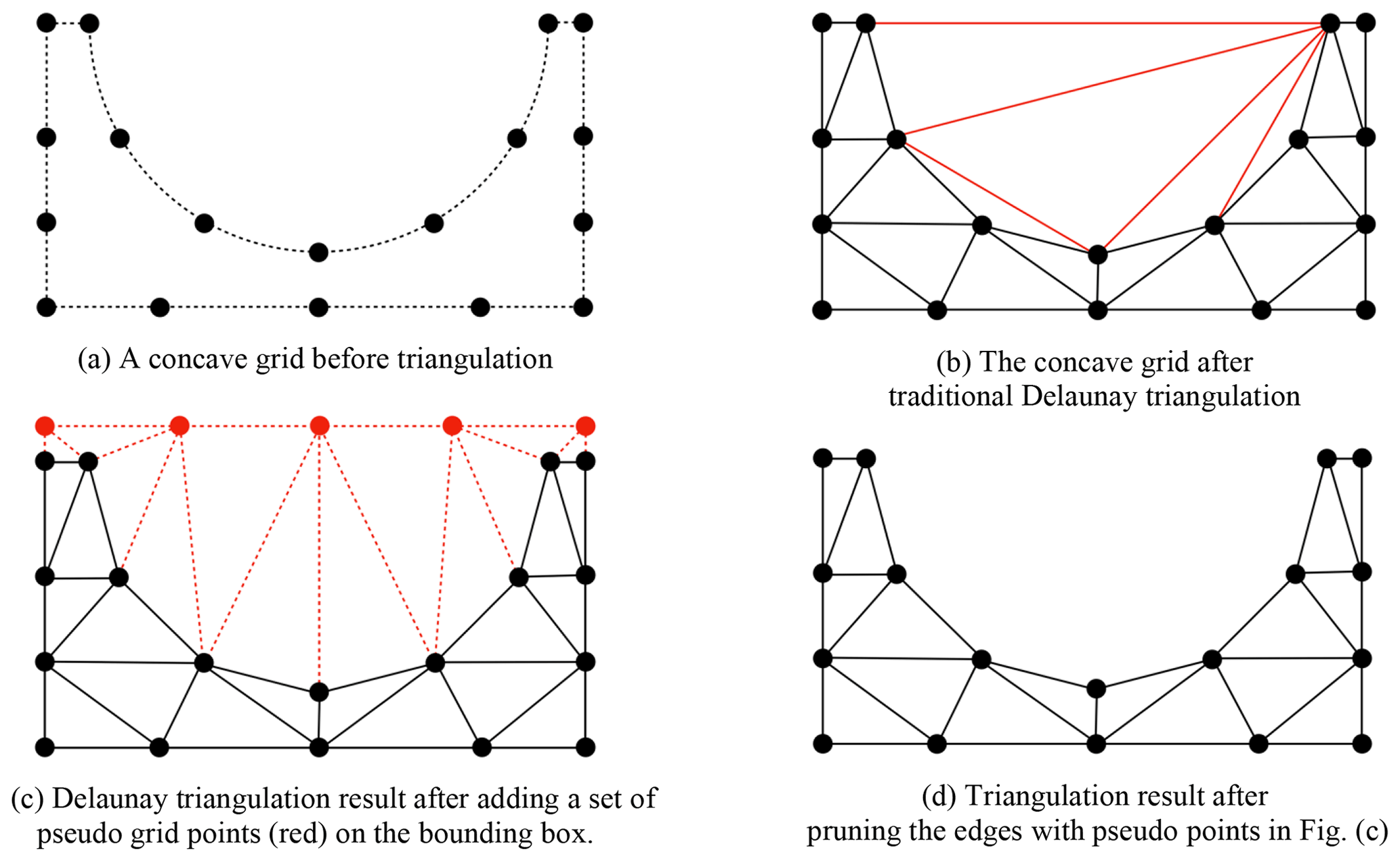
Given a regional (not global) spherical grid or a planar grid that is essentially a concave grid (e.g., the grid in Fig. 3a that has concave boundaries), as the Delaunay triangulation algorithm cannot handle a concave grid, false triangles will be obtained after triangulation (e.g., the red triangles in Fig. 3b). When designing PatCC1, we found that it is difficult to design a strategy to remove these false triangles. To address this challenge, a set of pseudo grid points on a bounding box of the regional grid is added, which can avoid the generation of false triangles (e.g., the result of triangulation in Fig. 3c). After removing the pseudo edges containing pseudo grid points, the result of triangulation can embody the profile of the concave boundaries (e.g., the result in Fig. 3d).
4.2 Computing resource manager
When using a hybrid of MPI and OpenMP for parallelization, a unique processor core (called a computing resource unit hereafter) is generally associated with a unique thread that belongs to an MPI process. Therefore, the pair MPI process ID and ID of the thread in the MPI process can be used to identify each computing resource unit. The computing resource manager records all computing resource units in an array, where the threads or MPI processes within the same computing node of a high-performance computer correspond to continuous elements in the array. To facilitate the search of computing resource units, the array index is used as the ID of each computing resource unit.
To achieve uniform implementation of parallelization with an MPI and OpenMP hybrid, the computing resource manager provides functionalities of communication between different computing resource units. If two computing resource units are two threads belonging to the same MPI process, the communication between them will be achieved through their shared memory space; otherwise, the communication will be achieved by MPI calls.
As the use of more computing resource units does not necessarily mean faster triangulation, e.g., when many computing resource units are available for an insufficiently large number of points in the whole grid, PatCC1 will select a part of the computing resource units for triangulation with the aim of near-optimal parallel performance. To achieve this, the computing resource manager first determines the maximum number of computing resource units according to the number of points in the whole grid and a threshold of the minimum number of points in each subgrid domain (which can be specified by the user). When the maximum number is smaller than the number of available computing resource units, the computing resource manager will select the same ratio of computing resource units from each computing node. For example, for 1000 available computing resource units where each computing node includes 20 computing resource units, when the maximum number is 500 then 500 computing resource units will be selected, with each computing node contributing 10 computing resource units.
4.3 Grid decomposition
The grid decomposition of PatCC1 includes two stages. The first is simultaneously to decompose the whole grid into a set of seamless and nonoverlapping subgrid domains (called kernel subgrid domains hereafter), assign each kernel subgrid domain to a computing resource unit, and build a tree for searching kernel subgrid domains. The second stage produces expanded subgrid domains through properly enlarging each kernel subgrid domain so that at least two expanded subgrid domains will cover a common boundary between kernel subgrid domains, and thus parallel consistency can be checked after the triangulation of the expanded subgrid domains is finished. In the following context, the first and second stages are called kernel decomposition and domain expansion, respectively.
A primary goal of grid decomposition is to achieve balanced triangulation times among subgrid domains. Although it is difficult or even impossible to achieve absolutely balanced times, we can design a simple heuristic according to the number of points in a subgrid domain because the time complexity of triangulation depends on the number of points. The grid decomposition therefore will try to achieve a similar number of points among kernel or expanded subgrid domains. To facilitate the triangulation for a polar region, the subgrid domain covering the pole will be circular, while the remaining grid domain that does not cover any pole will be decomposed into a set of rectangles (given a spherical grid, rectangles are defined in longitude–latitude space), as mentioned in Sect. 3. To avoid narrow rectangles, the grid decomposition should try to achieve a reasonable ratio (e.g., as close to 1 as possible) of the lengths of the edges of each rectangular subgrid domain. To avoid the additional work of handling cyclic boundary conditions in triangulation, a cyclic grid domain will be decomposed into a set of (at least two) acyclic rectangular subgrid domains. Therefore, a global grid will be decomposed into at least four subgrid domains, even when there are fewer than four computing resource units.
Figure 4 shows the pseudocode of the grid decomposition, where the procedure decompse_whole_grid corresponds to kernel decomposition. This procedure takes the whole grid after preprocessing (pseudo points have been added) and the active computing resource units that have been selected by the computing resource manager as inputs. The free computational capacity of each computing resource unit will be initialized to the number of grid points per computing resource unit (shortened to average point number hereafter), and will be decreased accordingly when a kernel subgrid domain is assigned to a computing resource unit. A computing resource unit without free computation capacity will no longer be considered in grid decomposition. The procedure decompse_whole_grid first generates at most two circular kernel subgrid domains with centers at the two poles according to the average point number, whenever the model grid covers either or both poles. Each circular kernel subgrid domain is assigned to a computing resource unit and will be inserted into the search tree of kernel subgrid domains.
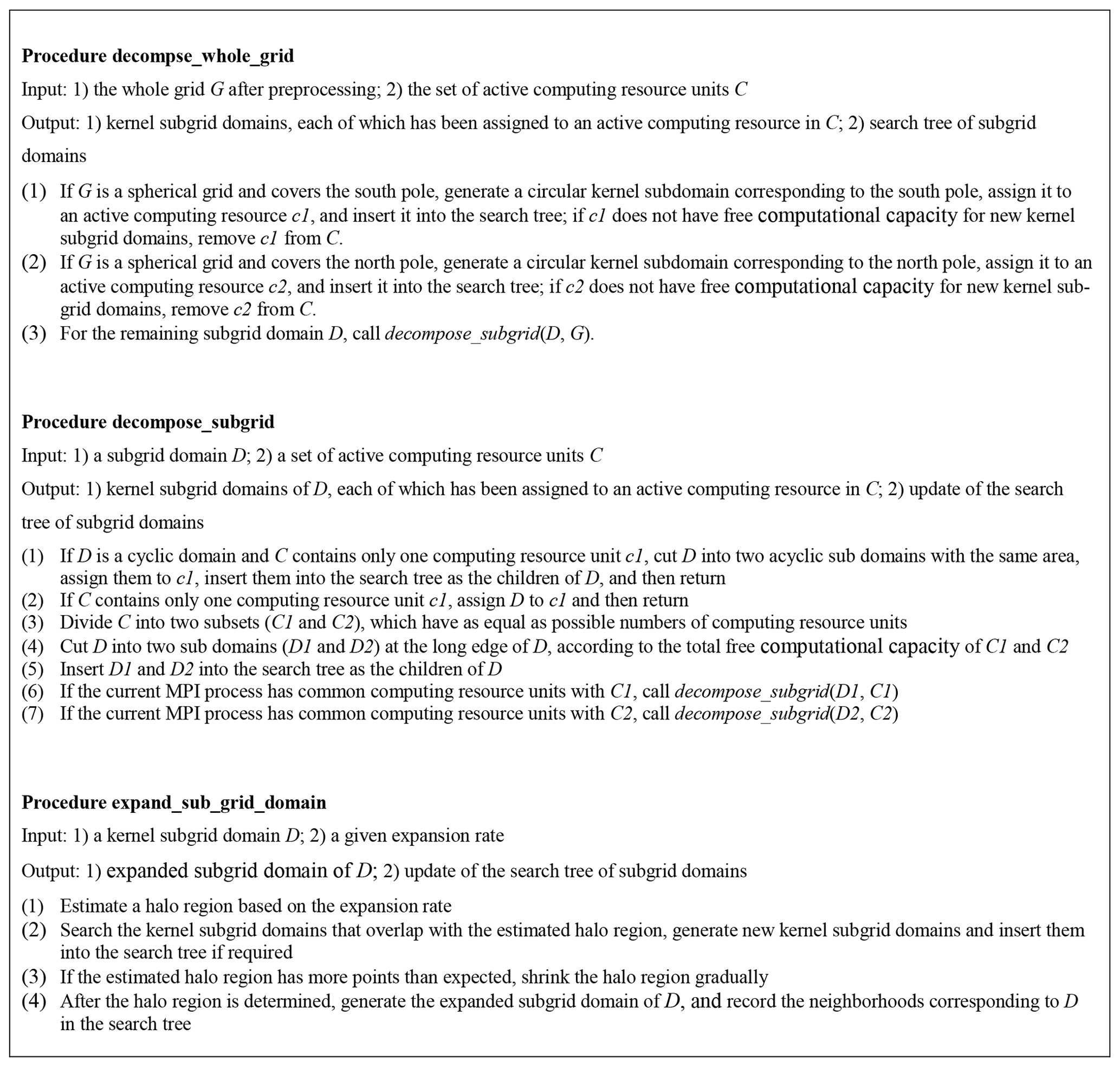
The procedure decompse_whole_grid next calls the procedure decompse_subgrid, which recursively decomposes a given rectangular grid domain for a given set of computing resource units with successive IDs (called a computing resource set). A cyclic grid domain will be divided into two acyclic subgrid domains with the same area even when the given computing resource set contains only one computing resource unit. If there is only one computing resource unit, the given rectangular subgrid domain will be assigned to it. Otherwise, the given computing resource set will be divided into two nonoverlapping subsets with balanced total free computational capacity, and two nonoverlapping rectangular subgrid domains will be generated accordingly (their point numbers will be balanced according to the total free computational capacity of the two computing resource subsets) through cutting the given rectangular grid domain at the long edge. For example, given a rectangular grid domain with 6000 points and a set of five computing resource units (no. 1–no. 5) with the same free computational capacity, the two computing resource subsets will include three (no. 1–no. 3) and two (no. 4 and no. 5) computing resource units, and thus the two rectangular subgrid domains will contain about 3600 and 2400 points, respectively. Next, the MPI processes that have common computing resource units with the first (second) computing resource subset will recursively decompose the first (second) rectangular subgrid domain, recursively. At each recursion, the newly generated subgrid domains will be inserted into the domain search tree as the children of the given grid domain.
The procedure expand_sub_grid_domain in Fig. 4 corresponds to the domain expansion stage. It is responsible for the expansion of a given kernel subgrid domain that has been assigned to the current computing resource unit (a computing resource unit will call this procedure several times when multiple kernel subgrid domains have been assigned to it). It first estimates a halo region for expansion based on an expansion rate (the ratio between the numbers of points after and before expansion) that can be specified by the user and then searches the kernel subgrid domains overlapping with the halo region from the domain search tree. (The search tree will be adaptively updated through a procedure (not shown) similar to the procedure decompose_subgrid when it does not include a kernel subgrid domain that overlaps with the halo region.) At the same time as generating an expanded subgrid domain, all neighboring kernel subgrid domains of the given kernel subgrid domain will be recorded.
The above design and implementation can be viewed as a procedure of constructing a specific k–d tree (Bentley, 1975) in longitude–latitude space for grid decomposition. They achieve balanced grid decomposition (balanced numbers of grid points) among the active computing resource units in most cases, and achieve a low time complexity of O(N) for an MPI process, because the overall domain search tree is almost a binary tree and an MPI process is generally only concerned with a limited number of top-down paths in the tree.
4.4 Local triangulation
As introduced in Sect. 3, we prefer to use a 2-D algorithm in local triangulation. Such an algorithm can directly handle the triangulation of planar grids, while it is necessary to project each subdomain of a spherical grid onto a plane before conducting 2-D triangulation. Similar to the Jacobsen algorithm, the local triangulation of PatCC1 also utilizes stereographic projection because the Delaunay triangulations on a spherical surface and on its stereographic projection surface are equivalent (Saalfeld, 1999). Our implementation, for a spherical grid, first sets the projection point to the point antipodal to the center of each spherical subgrid domain, generates the stereographic projection, and then applies the planar Delaunay triangulation process to the projected points.
For the triangulation process, we developed a divide-and-conquer-based recursive implementation, which in general achieves a time complexity of O(NlogN). A recursion of the triangulation implementation is to triangulate the points within a triangular domain. It first finds a point that is near to the center of the triangular domain and next divides the triangular domain into two or three smaller triangular domains. Legalization of triangles will be conducted when an illegal triangle is generated (in the Delaunay triangulation, a triangle is illegal if another point is within the circumcircle of the triangle). To avoid frequent memory allocation/deallocation operations that will greatly increase overhead, especially for parallel programs, an optimization of the memory pool is implemented, which efficiently manages the memory usage during triangulation.
There will be multiple legal solutions of Delaunay triangulation in cases having more than three points at the same circle, a situation that is unavoidable or even normal for model grids. When a circle that contains more than three points is in the overlapping region between two expanded subgrid domains after grid decomposition, local triangulation of the two expanded subgrid domains may produce different results corresponding to the overlapping region, which means that the triangulation of the whole grid will fail to achieve parallel consistency. A policy was therefore designed and used in the local triangulation to guarantee parallel consistency: given that the four points of two neighboring triangles (that share two points) are at the same circle, triangulation is legal only when the unique leftmost point or the lower-left point (if there are two leftmost points) are not shared by the two triangles (original coordinate values before projection will be used for determining the unique leftmost point or the lower-left point). Figure 5 shows an example demonstrating this policy. The triangulation in Fig. 5a is illegal because P1 is the unique leftmost point but is shared by the two triangles. Figure 5b shows the corresponding legal triangulation. In Fig. 5c, both P1 and P2 are leftmost points, while P2 is the lower left point. As P2 is shared by the two triangles, the triangulation in Fig. 5c is illegal. Figure 5d shows the corresponding legal triangulation.
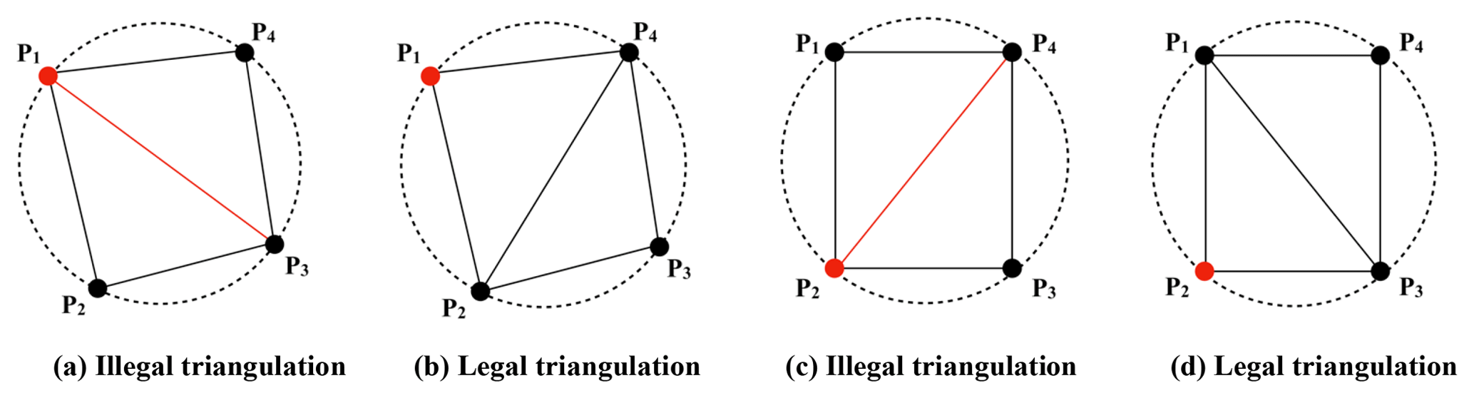
Figure 5Example demonstrating the policy for guaranteeing a unique triangulation solution. The four points P1–P4 in each graph (a–d) lie on the circumference of the same circle.
As a subgrid domain at a polar region is circular and covers the corresponding pole, significant load imbalance could be introduced after decomposing a latitude–longitude grid. For example, given a global latitude–longitude grid with 720×360 points and 1000 active computing resource units, the number of grid points per computing resource unit is about 259, while a polar subgrid domain must contain at least one latitude circle with 720 points. To address this problem, we developed a fast triangulation procedure (its time complexity is O(N)) specific for latitude–longitude grid domains, which will be used when a polar subgrid domain has been confirmed as a latitude–longitude grid domain.
4.5 Checking parallel consistency
PatCC1 will examine the parallel consistency of triangulation based on the overlapping regions among the expanded subgrid domains. When the local triangulations for any pair of overlapping expanded subgrid domains do not produce exactly the same triangles on the overlapping region, the triangulation for the whole grid fails to achieve parallel consistency. As the local triangulations for a pair of overlapping expanded subgrid domains are generally conducted separately by different computing resource units, data communication among computing resource units will be required for this step. To reduce the overhead of the data communication, only the triangles across a common boundary between two kernel subgrid domains are considered and a checksum corresponding to these triangles will be calculated and used for the check.
4.6 Merging all triangles
This main step is optional. It may be unnecessary when the result of triangulation will only be used for generating remapping weights in parallel because a computing resource unit generally can only consider the subgrid domains assigned to it in parallel remapping weight generation. This step is necessary when the overall triangulation result will be required, and has already been implemented in PatCC1 for evaluating whether PacCC1 achieves the parallel consistency. The root computing resource unit will gather all triangles within or across any boundary of each kernel subgrid domain from all active computing resource units and then prune repeated triangles (after passing the parallel consistency check, any pair of triangles with overlapping area are the same).
4.7 Parallelization with an MPI and OpenMP hybrid
To parallelize PatCC1 with an MPI and OpenMP hybrid, we try to parallelize each main step separately, as follows:
-
Preprocessing of the whole model grid. Parallelization of this step with MPI would introduce MPI data communication with a space complexity of O(N), where N is the number of points in the whole model grid; while the time complexity of this step is also O(N), this step is not parallelized with MPI to avoid MPI communication. In other words, each MPI process will preprocess the whole model grid. However, all OpenMP threads in an MPI process will cooperatively finish this step, which means that each OpenMP thread is responsible for preprocessing a part of the points in the whole model grid.
-
Initialization of the computing resource manager. This step will introduce collective communication among the MPI processes. It therefore cannot be accelerated through parallelization and more MPI processes generally means a higher overhead for this step.
-
Grid decomposition. Similar to the first step, the first stage of this step, which decomposes the whole grid into kernel subgrid domains, is not parallelized with MPI, while all active OpenMP threads in an MPI process will cooperatively decompose the whole grid. In detail, task-level OpenMP parallelization (corresponding to the OpenMP directive “#pragma omp task”) is utilized, where each OpenMP task corresponds to a function call of the procedure decompose_subgrid if its input subgrid domain contains enough points (i.e., the point number is larger than a given threshold). In the second stage of this step, each MPI process is responsible for expanding the subgrid domains that have been assigned to it while task-level OpenMP parallelization is further implemented. Therefore, the second stage has been parallelized with both MPI and OpenMP.
-
Local triangulation. Each computing resource unit is responsible for the local triangulation of the expanded subgrid domain assigned to it. Therefore, this step has been parallelized with both MPI and OpenMP.
-
Checking parallel consistency. Parallel consistency is simultaneously checked among different pairs of computing resource units corresponding to different pairs of overlapping expanded subgrid domains. Therefore, this step has been parallelized with both MPI and OpenMP.
-
Reconducting local triangulation for some subgrid domains after enlarging them. A computing resource unit is responsible for its assigned subgrid domains that fail to pass the parallel consistency check. Therefore, this step has been parallelized with both MPI and OpenMP.
-
Merging all triangles. This step will introduce collective communication among all active computing resource units. It therefore cannot be accelerated through parallelization and more active computing resource units or more points in the whole grid generally means a higher overhead for this step.
To minimize memory usage and synchronization among computing resource units, we prefer data parallelization for each step of PatCC1, where different computing resource units generally handle different subgrid domains. Considering that the subgrid domains to be decomposed dynamically change throughout the main recursive procedure of the grid decomposition (step 3), we implemented task-level OpenMP parallelization to achieve data parallelization, where all tasks correspond to the same procedure but different subgrid domains.
This section evaluates PatCC1 in terms of commonality, parallel efficiency, and parallel consistency. As the source code of the Jacobsen algorithm is publicly available (https://github.com/douglasjacobsen/MPI-SCVT, last access: 8 November 2018), we compared it with PatCC1. The parameter of expansion rate of PatCC1 is set to 1.2 throughout the evaluation.
5.1 Experimental setups
5.1.1 Computer platforms
Two computer platforms are used for evaluation: a shared-memory single-node server and a high-performance computer. The single-node server is equipped with two Intel Xeon E5-2686 18-core CPUs running at 2.3 GHz. Simultaneous multithreading (SMT) is enabled when using the single-node server and thus there are 36 physical processor cores and 72 logical process cores. Each computing node of the high-performance computer contains two Intel Xeon E5-2670 v2 10-core CPUs running at 2.5 GHz. SMT is not enabled on the high-performance computer and there are 20 physical (and thus also logical) processor cores in each computing node. Each computer platform provides enough main memory for evaluation.
Both the Jacobsen algorithm and PatCC1 are compiled with GNU compiler 4.8.5 under the optimization level O3 on either computer platform, and with the same Intel MPI library 3.2.2 on the single-node server and with the same Open MPI library 3.0.1 on the high-performance computer.
5.1.2 Model grids
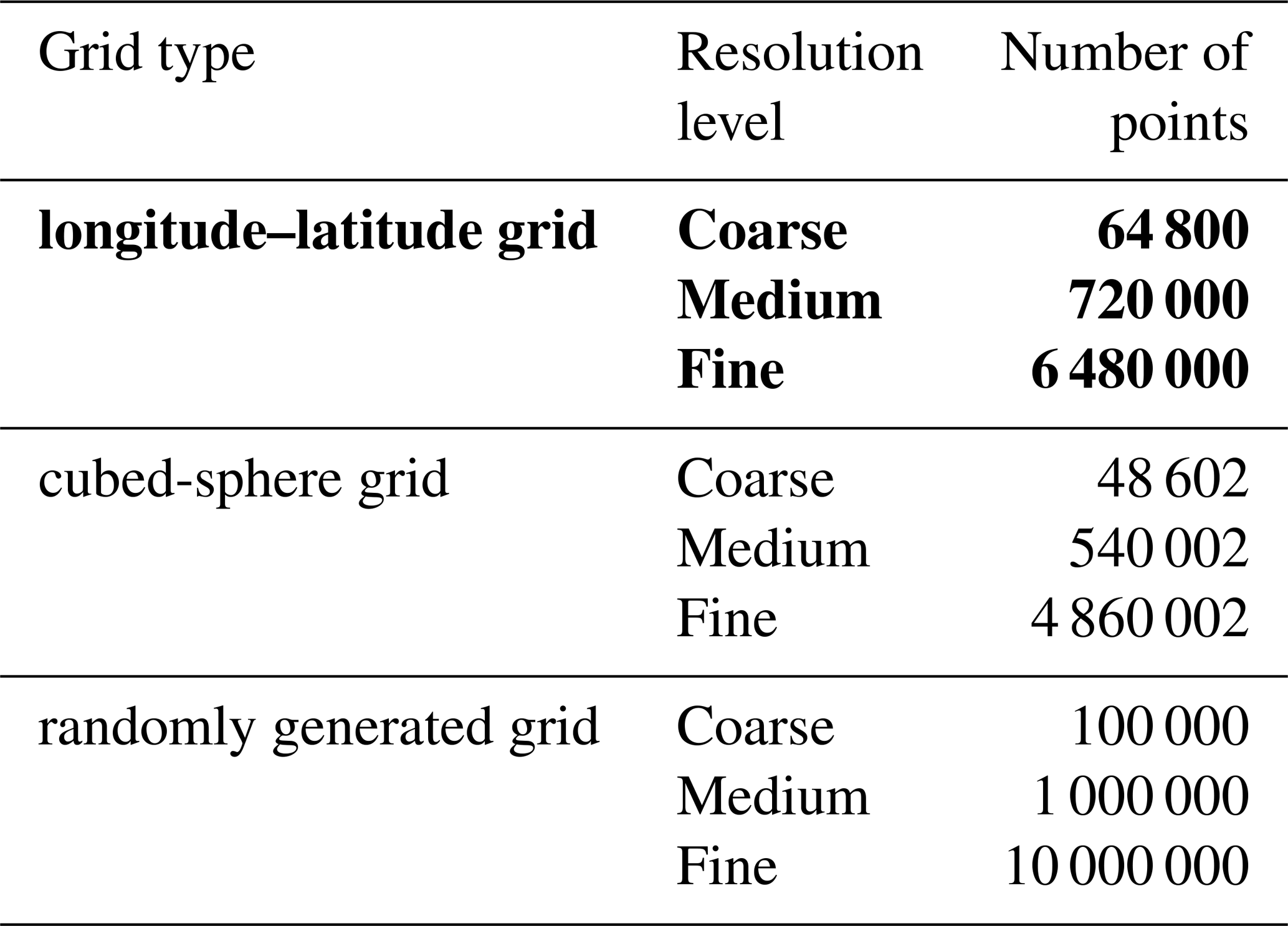
As shown in Table 1, a set of spherical grids from real models are used for evaluation: they are of different types and have different resolutions. Table 2 shows the generation of nine global grids based on three grid types (i.e., longitude–latitude grid, cubed-sphere grid, and randomly generated grid) and three levels of resolution (i.e., coarse, medium, and fine).
Table 1Set of spherical grids (from real models) of different types and with different resolutions.
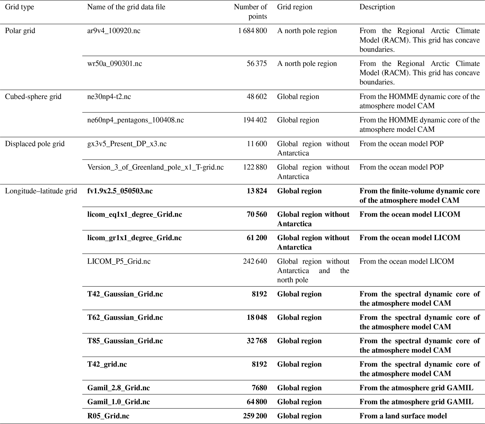
Table 2Set of global grids generated in the present study, based on three grid types and three resolution levels.
5.2 Evaluation of commonality and parallel consistency
An algorithm with commonality should successfully triangulate all grids in Tables 1 and 2. Given a whole grid, a successful triangulation should satisfy at least the following criteria:
-
The whole triangulation process finishes normally;
-
Each triangle is a legal Delaunay triangle and there is no overlapping area between any two triangles;
-
Given that any two grid points do not have the same coordinate values, every grid point is included in at least one triangle;
-
Each concave boundary (if any) in the original grid is retained after triangulation.
Following the above criteria, PatCC1 successfully triangulates all grids in both tables. Regarding the Jacobsen algorithm, it fails to triangulate all the longitude–latitude grids that cover at least one pole (shown in bold in Tables 1 and 2) because the triangulation process will exit abnormally when multiple points are at the same location on the sphere, and there are a number of points at each pole. It also fails to triangulate the polar grids in Table 1 with concave boundaries. As shown in Fig. 6, the Jacobsen algorithm will generate a number of false triangles above the concave boundaries, whereas PatCC1 does not generate any false triangles. The above results demonstrate that PatCC1 has much greater commonality than the Jacobsen algorithm.
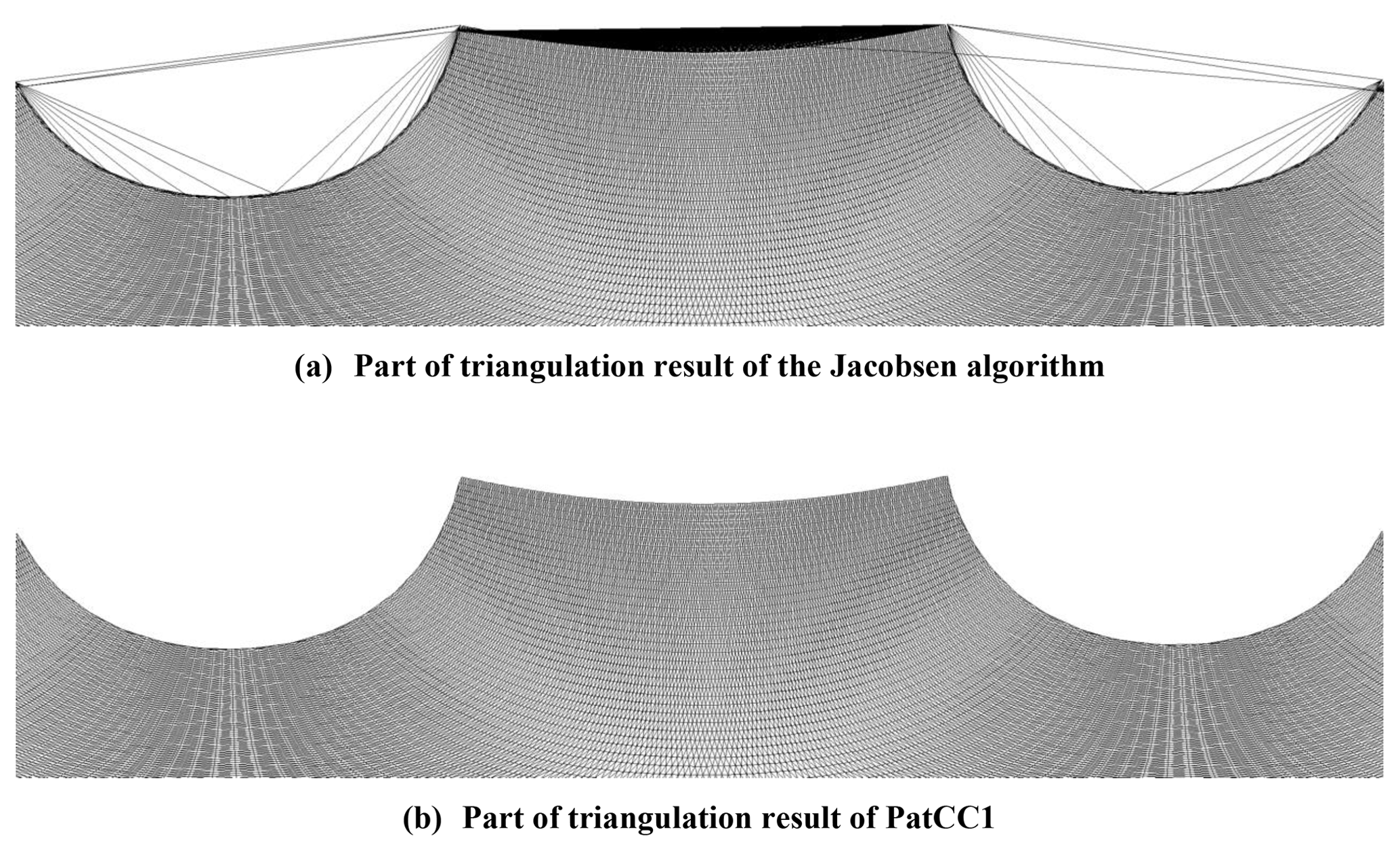
Figure 6Triangulation results for the polar grid ar9v4_100920.nc that contains concave boundaries.
To evaluate parallel consistency, the last main step of PatCC1 is enabled, and all triangles will be written into a binary data file after sorting them. All grids in both tables are used for this evaluation. At least four parallel settings are used for each grid (with different numbers of MPI processes or different numbers of OpenMP threads). The test results show that for each grid, the binary data files of triangles under all parallel settings are exactly the same. We therefore conclude that PatCC1 achieves parallel consistency.
5.3 Evaluation of parallel performance
5.3.1 Performance on the single-node server
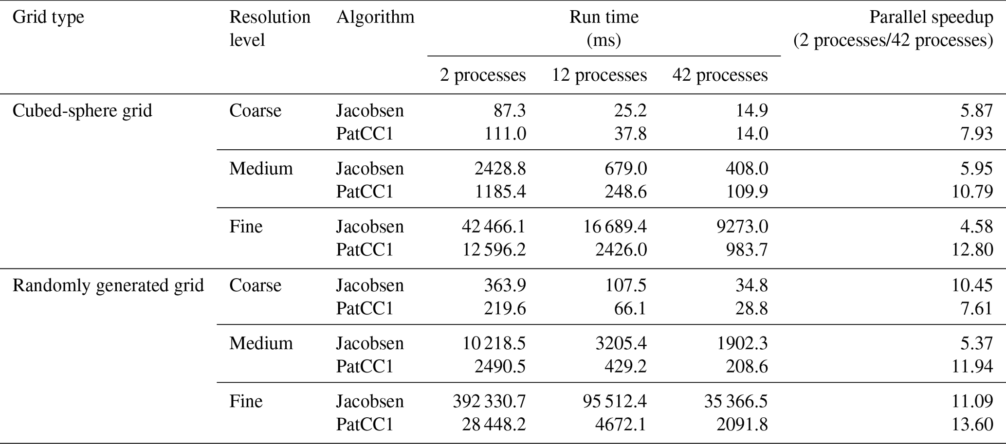
We first evaluate the parallel performance using all grids in Table 2 on the single-node server. When the total number of processes or threads does not exceed 36, each process or thread will be set to a unique physical core. As the Jacobsen algorithm will use offline grid decomposition information included in two predefined files (one containing a list of region centers for parallelization and the other containing the connectivity of the regions) and three pairs of these files for three parallel settings (2, 12, and 42 processes) are publicly available (https://github.com/douglasjacobsen/MPI-SCVT, last access: 8 November 2018), we use only these three parallel settings to run the Jacobsen algorithm. To compare the Jacobsen algorithm and PatCC1, we focus only on the time for local triangulation without considering the time for grid decomposition because the Jacobsen algorithm uses offline grid decomposition information while PatCC1 calculates grid decomposition information online. According to the test results in Table 3, PatCC1 is faster and achieves higher parallel speedup than the Jacobsen algorithm in most cases. Moreover, higher parallel speedup is achieved by PatCC1 for finer grid resolution.
Table 3Comparison of local triangulation times for the Jacobsen algorithm and PatCC1 under different numbers of total MPI processes. Only one OpenMP thread is enabled in each MPI process.
To further evaluate the parallel performance of PatCC1 on the single-node server, more parallel settings are used and the time is measured for each main step (except the last step because it is optional and cannot be parallelized). The test results corresponding to randomly generated grids, cubed-sphere grids, and longitude–latitude grids are shown in Tables 4–6, S1–S3, and S4–S6 (in the Supplement), respectively. The results lead to the following observations.
-
Concurrent running of MPI processes will degrade the performance of the first main step (for preprocessing the whole grid), and more MPI processes generally mean more significant degradation. As this step is memory bandwidth bound and has not been parallelized with MPI, the overall complexity of memory bandwidth requirement is O(MN), where M is the number of MPI processes and N is the number of grid points. Given M MPI processes, the increment of the run time is generally larger than 1 but much lower than an M-fold increase. This is because concurrent running of MPI processes enables the utilization of more memory bandwidth while the overall memory bandwidth capacity on a computing node is limited. Regarding OpenMP parallelization, a small parallel speedup (larger than 1) without performance degradation is obtained. This is because the overall complexity of the memory bandwidth requirement remains consistently O(N), and the concurrent running of OpenMP threads also enables the utilization of more memory bandwidth.
-
As the second main step (initiating the computing resource manager) will introduce collective communication among MPI processes, the overhead of this step increases with the increment of MPI processes, while the overhead remains almost constant with the increment of OpenMP threads.
-
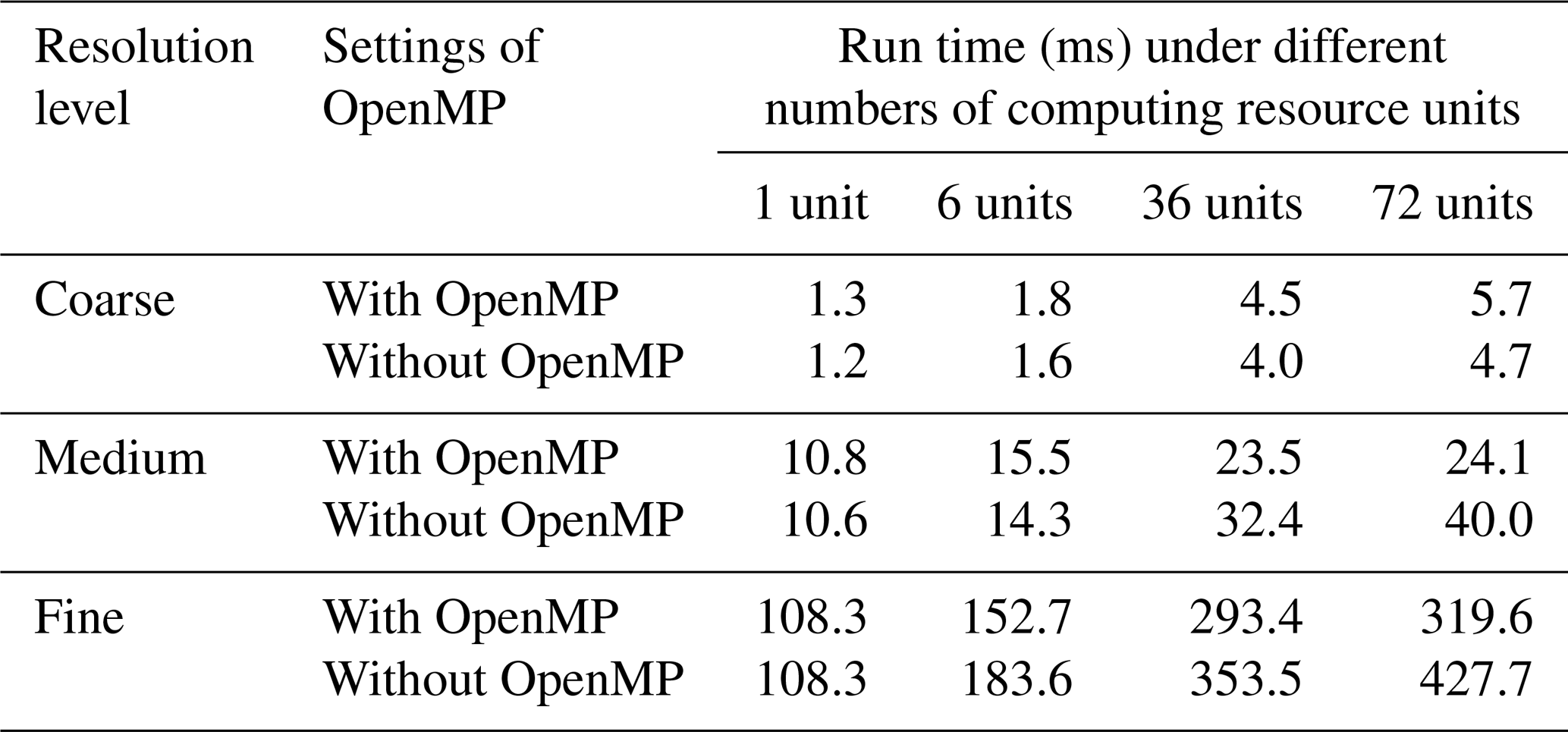
Similar to the first main step, the first stage of the third main step (decomposing the whole grid into kernel subdomains) suffers significant degradation when using more MPI processes. Although concurrent running of OpenMP threads can achieve a faster speed than the concurrent running of MPI processes when the resolution of the grids is medium or fine, more significant performance degradation is also observed when using more OpenMP threads. This is because the overall complexity of the memory bandwidth requirement under OpenMP-only parallelization is O(NlogM), where M is the number of OpenMP threads, the task-level OpenMP parallelization introduces some extra overhead, and the parallelism exploited is limited. As shown in Table 7, OpenMP parallelization actually accelerates this stage.
-
As the second stage of the third main step (expanding kernel subdomains) has been parallelized with both MPI and OpenMP, obvious speedup is obtained in concurrent running of MPI processes or OpenMP threads. Compared with MPI parallelization, OpenMP parallelization can avoid redundant grid decomposition among MPI processes (different kernel subdomains assigned to different MPI processes may have the same kernel subdomain as a neighbor) but will introduce the overhead of OpenMP task management and scheduling. As a result, OpenMP parallelization and MPI parallelization can outperform each other at different grid sizes (i.e., numbers of grid points).
-
As the fourth main step (local triangulation) has been parallelized with both MPI and OpenMP, obvious speedup is obtained in concurrent running of MPI processes or OpenMP threads. Although the same strategy of a computing resource unit only handling the local triangulation of the expanded subgrid domain that has been assigned to it is employed for both parallelizations, MPI parallelization outperforms OpenMP parallelization in most cases. One possible reason for this is that memory allocation is still necessary in local triangulation after the optimization of the memory pool is implemented, while concurrent MPI processes handle memory allocation generally more efficiently than concurrent threads.
-
Although parallelization with OpenMP or MPI does not achieve obvious parallel speedup for the fifth main step (checking parallel consistency), this step generally takes a small proportion of the overall execution time of parallel triangulation.
-
As SMT can effectively hide the latency from irregular memory access, while frequent irregular memory accesses are introduced by the pointer-based data structures of triangles, SMT provides additional parallel speedup for local triangulation in most cases.
-
Regarding the total execution time, OpenMP-only execution and MPI-only execution can outperform each other at different levels of grid sizes, while hybrid MPI–OpenMP execution generally achieves a moderate performance between the two.
Table 4Run time and parallel speedup of each main step of PatCC1 under different parallel settings, when using the randomly generated grid at the coarse-resolution level. “3-1” and “3-2” indicate the first stage (decompose the whole grid into kernel subgrid domains) and second stage (expand each kernel subgrid domain) of the third step, respectively. “MPIOpenMP” indicates that the number of MPI threads and the number of OpenMP threads in each MPI process are equal.
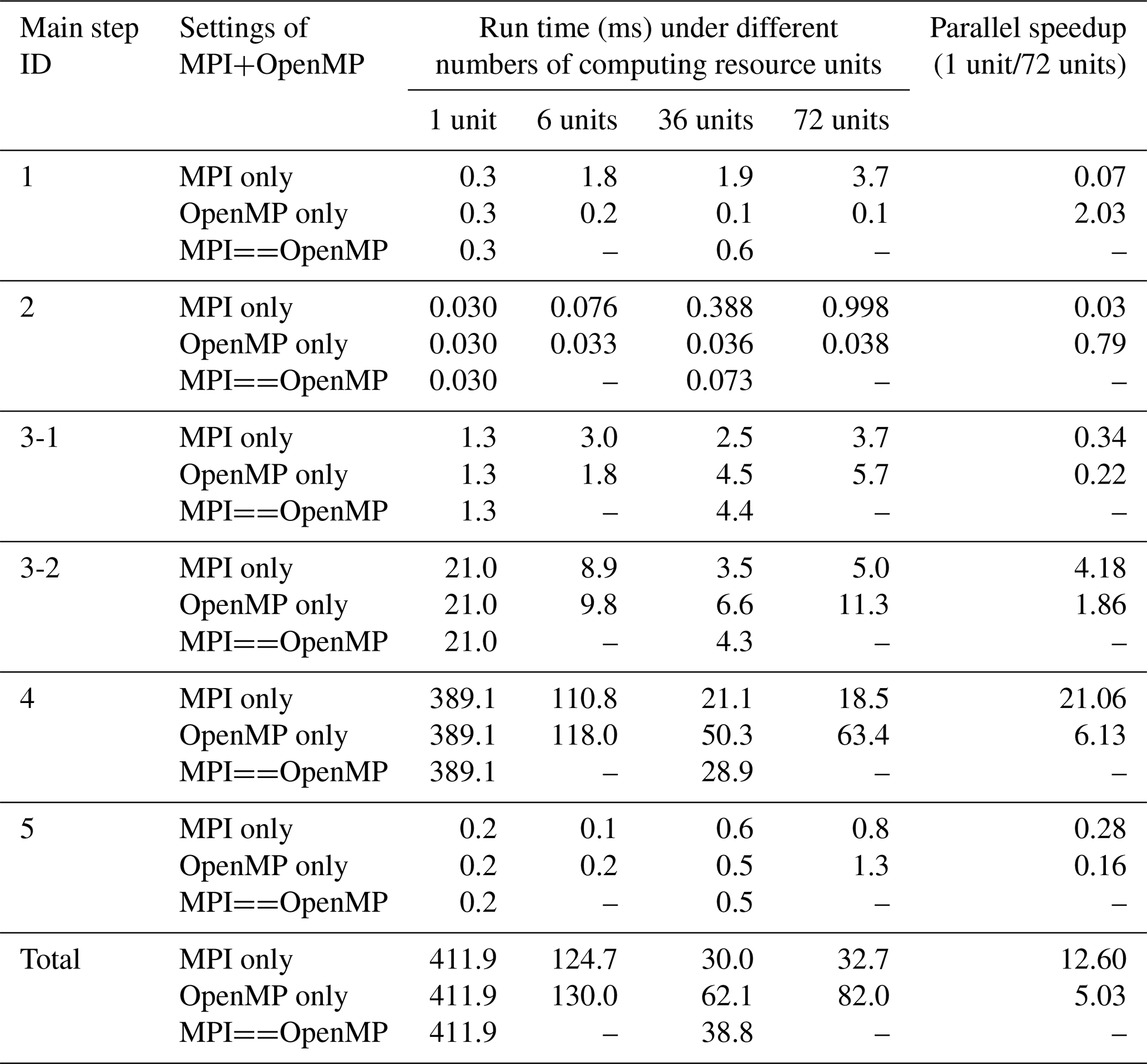
Table 5Run time and parallel speedup of each main step of PatCC1 under different parallel settings, when using the randomly generated grid at the medium resolution level. “3-1” and “3-2” indicate the first stage (decompose the whole grid into kernel subgrid domains) and second stage (expand each kernel subgrid domain) of the third step, respectively. “MPIOpenMP” indicates that the number of MPI threads and the number of OpenMP threads in each MPI process are equal.

Table 6Run time and parallel speedup of each main step of PatCC1 under different parallel settings, when using the randomly generated grid at the fine-resolution level. “3-1” and “3-2” indicate the first stage (decompose the whole grid into kernel subgrid domains) and second stage (expand each kernel subgrid domain) of the third step, respectively. “MPIOpenMP” indicates that the number of MPI threads and the number of OpenMP threads in each MPI process are equal.
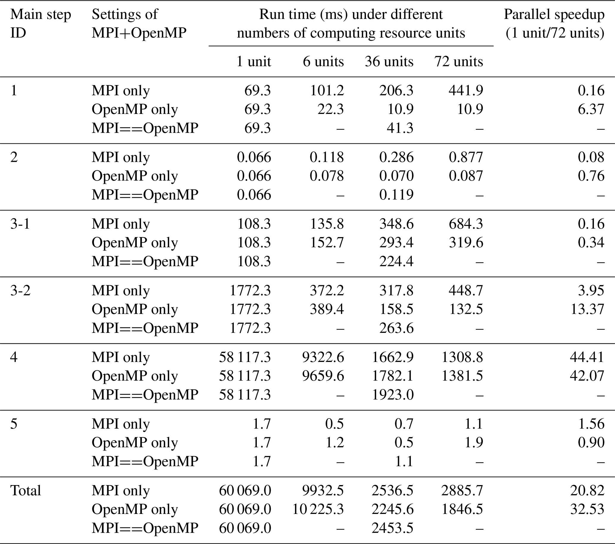
Table 7Run time of step 3-1 with and without OpenMP parallelization when using the randomly generated grid under different resolution levels.
5.3.2 Performance on the high-performance computer
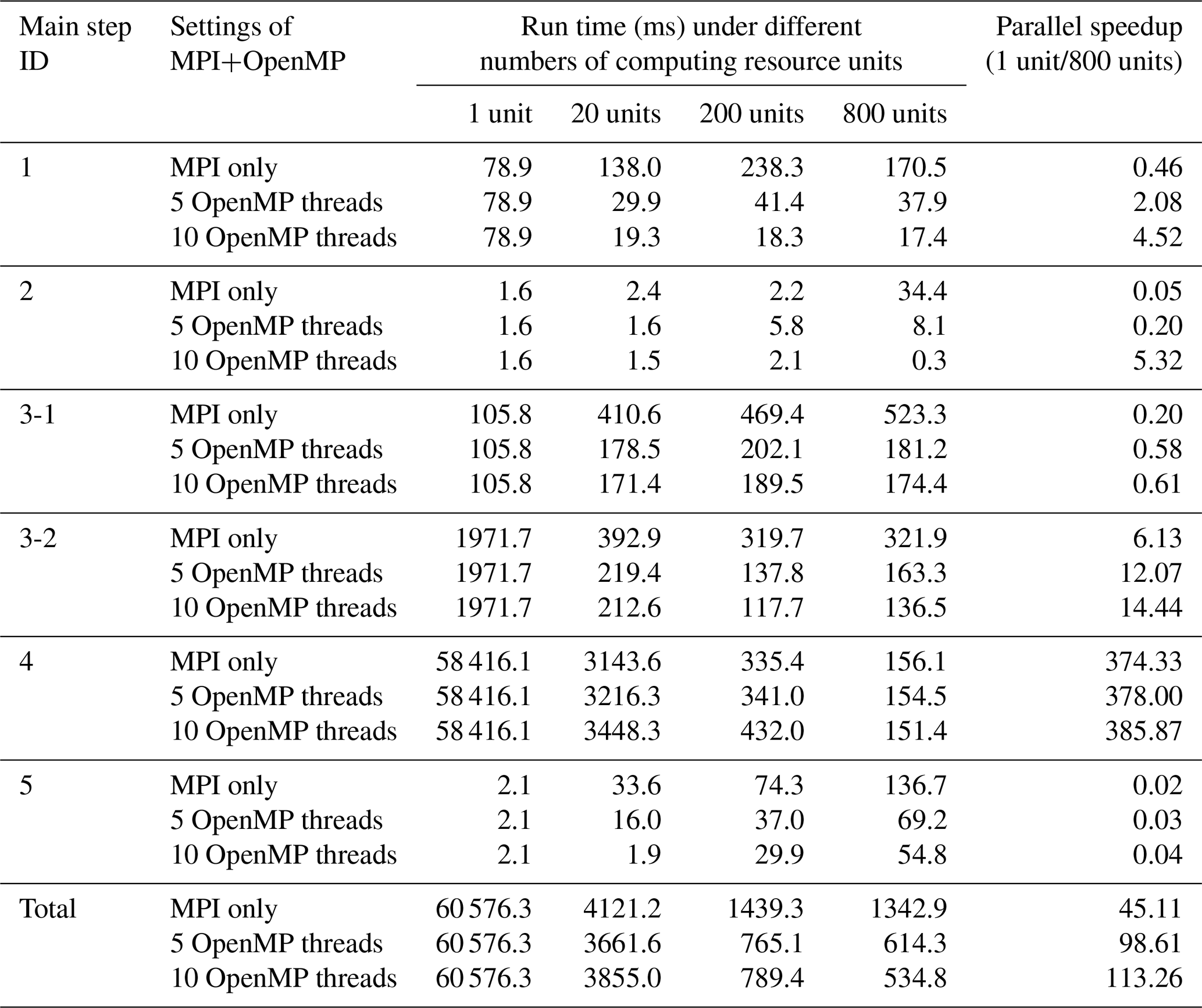
We next evaluate the parallel performance of PatCC1 using the fine grids in Table 2 on the high-performance computer. OpenMP is compared using 1, 5, and 10 threads, and the time for each main step (except the last step) is measured. The test results for the randomly generated grid, cubed-sphere grid and longitude–latitude grid are shown in Tables 8, S7, and S8 (in the Supplement), respectively. Each computing node contributes 10 processor cores when there are 20 computing resource units or more. For example, when there are 800 computing resource units, 80 computing nodes are used. In addition to the observations discussed in Sect. 5.3.1, we can make the following observations regarding the increment of computing nodes.
-
The execution time of the first main step remains almost constant with the increment of computing nodes because the requirement and capacity of the memory bandwidth corresponding to each computing node remain constant.
-
The cost of the second step increases with the number of computing resource units especially the number of processes because this step introduces collective communications among all computing resource units.
-
The execution time of the first stage of the third main step increases slightly with the increment of computing nodes because there will be more recursion levels in grid decomposition when more computing resource units are used.
-
The main step of local triangulation achieves significant parallel speedups. When using 800 processor cores, it achieves more than a 360-fold speedup for all fine grids.
-
The cost of parallel consistency check increases with the increment of computing nodes, and decreases when more OpenMP threads are used under the same number of computing resource units. This is because the parallel consistency check will introduce MPI communications among processes and the overhead of communications generally increases or decreases with the increment or decrement of processes.
Table 8Run time and parallel speedup of each main step of PatCC1 under different parallel settings, when using the randomly generated grid at the fine-resolution level. “3-1” and “3-2” indicate the first stage (decompose the whole grid into kernel subgrid domains) and second stage (expand each kernel subgrid domain) of the third step, respectively.
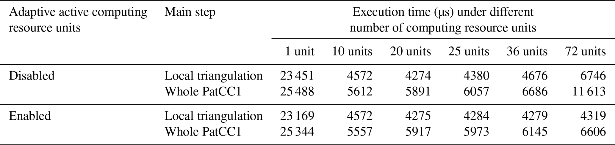
5.3.3 Impact of computing resource management
As introduced in Sect. 4.2, the computing resource manager can adaptively select a part of the computing resource units for triangulation when too many computing resource units are available. To evaluate the benefit of this functionality, we employ a randomly generated global grid with 2000 points and run PatCC1 on the single-node server under different numbers of MPI processes (MPI only). As shown in Table 9, when this functionality is disabled, after the MPI process number reaches 20, the execution times of local triangulation and the whole PatCC1 algorithm increase with further increases in MPI processes. When this functionality is enabled (the threshold of the minimum number of points in each subgrid domain is set to 100), after the MPI process number reaches 20, the execution times of both local triangulation and the whole PatCC1 algorithm increase only slightly. (The times for preprocessing the whole grid and initiating the computing resource manager still increase with the increment of MPI processes.)
Table 9Evaluation of the functionality of adaptively selecting a part of computing resource units for triangulation. A randomly generated global grid with 2000 points is used and PatCC1 is run on the single-node server under different numbers of computing resource units (MPI only).
This paper proposes a new parallel triangulation algorithm, PatCC1, for spherical and planar grids. Experimental evaluation employing comparison with a state-of-the-art method and using different sets of grids and two computer platforms demonstrates that PatCC1, which has been parallelized with a hybrid of MPI and OpenMP, is an efficient parallel triangulation algorithm with commonality and parallel consistency.
C-Coupler1 and C-Coupler2 have already employed a sequential Delaunay triangulation algorithm for the management of horizontal grids. When cell vertexes of a horizontal grid are not provided, they can be automatically generated from the Voronoi diagram based on the triangulation and further used by nonconservative remapping algorithms (the couplers will force users to provide real cell vertexes of grids involved in conservative remapping). Our future work will replace the sequential triangulation algorithm in C-Coupler2 (the latest version of C-Coupler) by PatCC1 so as to develop the next coupler version (C-Coupler3), which is planned to be finished and released before the end of 2021.
Calculations for the position of a point to a line (on the line or not) or to the circumcircle of a triangle (on, in, or out of the circle) are fundamental operations in local triangulations. Due to the round-off errors from floating-point calculations, accurate conditions cannot be employed for such calculations and thus error-tolerant conditions are developed. For example, a point will be judged on a circle if the ratio between the distance from the point to the circle and the radius of the circle is within the corresponding tolerant error. Our experiences have shown that improper tolerant errors introduce failures of triangulation to some grids. Without theoretical guides, the tolerant errors in PatCC1 have to be set empirically, i.e., no failed triangulation in all test cases generally mean a proper setting of the tolerant errors. In the future, more test cases with more grids will be designed for bettering the setting of tolerant errors.
An improper setting of the expansion rate can introduce performance reduction to PatCC1. When the expansion rate gets bigger, an expansion will produce bigger overlapping regions among expanded subgrid domains, which will result in higher overhead in local triangulations; when the expansion rate gets smaller, failures of the parallel consistency check may be increased, which will also slow down the whole algorithm. The expansion rate currently is a constant value in PatCC1 that can be specified by users. In the future, we will investigate how to automatically determine its proper values.
When developing the OpenMP parallelization, we preferred to develop coarse-grained rather than fine-grained parallelization to minimize code modification. Such an OpenMP parallelization achieves obvious parallel speedup for most of the main steps of PatCC1, except the first stage of grid decomposition. We tried to develop a fine-grained OpenMP parallelization for this stage, but without success because it requires modification of the kernel algorithm which would thus degrade the performance.
When using a small number of computing resource units, the main step of local triangulation generally takes most of the execution time of the whole PatCC1 algorithm because the time complexity of each other step is lower. With the increment of computing resource units, the local triangulation is accelerated dramatically, while the nonscalable and low-time-complexity steps (e.g., preprocessing of the whole grid and grid decomposition) gradually become bottlenecks. Our future work will investigate the acceleration of these steps, especially when the grid is extremely large and many computing resource units are used.
The computer platforms used for evaluation in this paper are heterogeneous. To make PatCC1 adapt to a homogeneous computer platform where processor cores have different computing powers, the free computational capacity of each computing resource unit can be initialized according to its computing power.
The source code of PatCC1 is generally free for noncommercial activities and a version of the source code can be downloaded via https://doi.org/10.5281/zenodo.3249835 (WireFisher, 2019). Regarding commercial usage, please contact us first for the permission.
The supplement related to this article is available online at: https://doi.org/10.5194/gmd-12-3311-2019-supplement.
HY was responsible for code development, software testing, and experimental evaluation of PatCC1 and co-led paper writing. LL initiated this research, proposed most ideas, supervised HY, and co-led paper writing. RL will be responsible for code release and technical support of PatCC1 after HY's graduation. All authors contributed to improvement of ideas, software testing, experimental evaluation, and paper writing.
The authors declare that they have no conflict of interest.
This work was jointly supported in part by the National Key Research Project of China (grant nos. 2016YFA0602203 and 2017YFC1501903). We would like to thank Douglas Jacobsen et al. for the source code of the Jacobsen algorithm that is publicly available through GitHub. We also thank the editor and the reviewers for handling this paper.
This research has been supported by the National Key Research Project of China (grant nos. 2016YFA0602203 and 2017YFC1501903).
This paper was edited by Olivier Marti and reviewed by two anonymous referees.
Bentley, J. L.: Multidimensional binary search trees used for associative searching, Commun. ACM, 18, 509–517, 1975.
Craig, A., Valcke, S., and Coquart, L.: Development and performance of a new version of the OASIS coupler, OASIS3-MCT_3.0, Geosci. Model Dev., 10, 3297–3308, https://doi.org/10.5194/gmd-10-3297-2017, 2017.
Craig, A. P., Jacob, R. L., Kauffman, B., Bettge, T., Larson, J. W., Ong, E. T., Ding, C. H. Q., and He, Y.: CPL6: The New Extensible, High Performance Parallel Coupler for the Community Climate System Model, Int. J. High Perform. C, 19, 309–327, 2005.
Craig, A. P., Vertenstein, M., and Jacob, R.: A New Flexible Coupler for Earth System Modeling developed for CCSM4 and CESM1, Int. J. High Perform. C, 26-1, 31–42, https://doi.org/10.1177/1094342011428141, 2012.
Guibas, L. and Stolfi, J.: Primitives for the manipulation of general subdivisions and the computation of Voronoi, ACM T. Graphic., 4, 74–123, 1985.
Hanke, M., Redler, R., Holfeld, T., and Yastremsky, M.: YAC 1.2.0: new aspects for coupling software in Earth system modelling, Geosci. Model Dev., 9, 2755–2769, https://doi.org/10.5194/gmd-9-2755-2016, 2016.
Hill, C., DeLuca, C., Balaji, V., Suarez, M., and da Silva, A.: Architecture of the Earth System Modeling Framework, Comput. Sci. Eng., 6, 18–28, 2004.
Jacobsen, D. W., Gunzburger, M., Ringler, T., Burkardt, J., and Peterson, J.: Parallel algorithms for planar and spherical Delaunay construction with an application to centroidal Voronoi tessellations, Geosci. Model Dev., 6, 1353–1365, https://doi.org/10.5194/gmd-6-1353-2013, 2013.
Jones, P.: Conservative remapping: First- and second-order conservative remapping, Mon. Weather Rev., 127, 2204, https://doi.org/10.1175/1520-0493(1999)127<2204:FASOCR>2.0.CO;2, 1999.
Larrea, V. G. V.: Construction of Delaunay Triangulations on the Sphere: A Parallel Approach, Master thesis, 2011.
Larson, J., Jacob, R., and Ong, E.: The Model Coupling Toolkit: A New Fortran90 Toolkit for Building Multiphysics Parallel Coupled Models, Int. J. High Perform. C, 19, 277–292, https://doi.org/10.1177/1094342005056116, 2005.
Liu, L., Yang, G., Wang, B., Zhang, C., Li, R., Zhang, Z., Ji, Y., and Wang, L.: C-Coupler1: a Chinese community coupler for Earth system modeling, Geosci. Model Dev., 7, 2281–2302, https://doi.org/10.5194/gmd-7-2281-2014, 2014.
Liu, L., Zhang, C., Li, R., Wang, B., and Yang, G.: C-Coupler2: a flexible and user-friendly community coupler for model coupling and nesting, Geosci. Model Dev., 11, 3557–3586, https://doi.org/10.5194/gmd-11-3557-2018, 2018.
Prill, F. and Zängl, G.: A Compact Parallel Algorithm for Spherical Delaunay Triangulations, Concurrency and Computation Practice and Experience, 29, 355–364, https://doi.org/10.1002/cpe.3971, 2016.
Redler, R., Valcke, S., and Ritzdorf, H.: OASIS4 – a coupling software for next generation earth system modelling, Geosci. Model Dev., 3, 87–104, https://doi.org/10.5194/gmd-3-87-2010, 2010.
Saalfeld, A.: Delaunay Triangulations and Stereographic Projections, Am. Cartographer, 26, 289–296, 1999.
Su, P. and Drysdale, R. L. S.: A comparison of sequential Delaunay triangulation algorithms, Elsevier Science Publishers B. V., 1997.
Valcke, S.: The OASIS3 coupler: a European climate modelling community software, Geosci. Model Dev., 6, 373–388, https://doi.org/10.5194/gmd-6-373-2013, 2013.
Valcke, S., Balaji, V., Craig, A., DeLuca, C., Dunlap, R., Ford, R. W., Jacob, R., Larson, J., O'Kuinghttons, R., Riley, G. D., and Vertenstein, M.: Coupling technologies for Earth System Modelling, Geosci. Model Dev., 5, 1589–1596, https://doi.org/10.5194/gmd-5-1589-2012, 2012.
WireFisher: WireFisher/PatCC: v1.0.0 (Version v1.0.0), Zenodo, https://doi.org/10.5281/zenodo.3249835, 2019.