The multiscale routing model mRM v1.0: simple river routing at resolutions from 1 to 50 km

Routing streamflow through a river network is a fundamental requirement to verify lateral water fluxes simulated by hydrologic and land surface models. River routing is performed at diverse resolutions ranging from few kilometres to 1^∘. The presented multiscale routing model mRM calculates streamflow at diverse spatial and temporal resolutions. mRM solves the kinematic wave equation using a finite difference scheme. An adaptive time stepping scheme fulfilling a numerical stability criterion is introduced in this study and compared against the original parameterisation of mRM that has been developed within the mesoscale hydrologic model (mHM). mRM requires a high-resolution river network, which is upscaled internally to the desired spatial resolution. The user can change the spatial resolution by simply changing a single number in the configuration file without any further adjustments of the input data. The performance of mRM is investigated on two datasets: a high-resolution German dataset and a slightly lower resolved European dataset. The adaptive time stepping scheme within mRM shows a remarkable scalability compared to its predecessor. Median Kling–Gupta efficiencies change less than 3 % when the model parameterisation is transferred from 3 to 48 km resolution. mRM also exhibits seamless scalability in time, providing similar results when forced with hourly and daily runoff. The streamflow calculated over the Danube catchment by the regional climate model REMO coupled to mRM reveals that the 50 km simulation shows a smaller bias with respect to observations than the simulation at 12 km resolution. The mRM source code is freely available and highly modular, facilitating easy internal coupling in existing Earth system models.

1 Introduction

Streamflow provides an integrated signal of lateral hydrologic fluxes at the land surface over a catchment area. Streamflow observations are routinely used within hydrologic modelling to perform model characterisation or calibration and validation (Beven, 2012). Comparisons between simulated and observed streamflow are typically conducted using measures focusing on daily values (Nash and Sutcliffe, 1970; Gupta et al., 2009). Similarly to hydrologic models (HMs), land surface models (LSMs) also represent the terrestrial hydrologic cycle. They additionally include the terrestrial energy budget and biogeochemical cycles, such as the carbon cycle, to provide the exchange fluxes of the land surface with the atmosphere in, for example, regional circulation models (RCMs) or Earth system models (ESMs). Streamflow is estimated in ESMs to provide fresh water input of the land surface into the ocean (Sein et al., 2015). Streamflow observations are also used in land surface models in the context of climate studies to validate the hydrologic cycle at daily (among others, Marx et al., 2018; Thober et al., 2018; Samaniego et al., 2018), monthly (among others, Hagemann et al., 2009; Li et al., 2015; Zhang et al., 2016) or even annual timescales (among others, Zhou et al., 2012).

Hydrologic models (HMs) and land surface models (LSMs) are historically run at different spatial resolutions. HMs are, for instance, applied at scales of few kilometres and less, even in continental-scale applications (Wood et al., 2011; Marx et al., 2018; Thober et al., 2018; Samaniego et al., 2018; Wanders et al., 2019), whereas LSMs are applied at resolutions of tens of kilometres and more within climate change studies (Van der Linden and Mitchell, 2009; Taylor et al., 2012). However, a substantial increase in model resolution has been achieved for regional circulation models (RCMs) in the past years and these are run nowadays at different resolutions down to the convection-permitting scale of a few kilometres (Jacob et al., 2014). Applying RCMs at diverse resolutions implies that the same LSM (i.e. the same representation of water, energy, and biogeochemical processes) is used on diverse resolutions. This imposes a challenge on the LSM parameterisations to be able to represent all included processes at the different resolutions (Wood et al., 1998; Haddeland et al., 2002; Boone et al., 2004). The main goal of this study is to provide LSMs that do not include a river routing scheme, with a framework to compute streamflow for comparison against observations. The distinctive property of this framework is that the spatial resolution can be easily changed by the user without any modification to the model setup.

River routing is the process of predicting the hydrograph evolution as runoff moves through a river network. It can be described at different levels of complexity. The general governing equation of this phenomenon is the unidimensional Saint-Venant equations (de Saint-Venant, 1871). Models using the Saint-Venant equations are referred to as hydraulic models that are especially suited if backwater effects occur such as in flat regions or river deltas (Paiva et al., 2011; Miguez Macho and Fan, 2012; Paiva et al., 2013; Yamazaki et al., 2013). These models exploit remote sensing to derive model parameters and setup (Neal et al., 2012; Beighley et al., 2009). If rivers are steep enough and relatively shallow, simplification of the Saint-Venant equations such as the kinematic wave equation is sufficient (Lohmann et al., 1996; Hagemann and Dümenil, 1997; Todini, 2007). They require less information about river topography and only account for wave advection and attenuation. These models are not applicable for large river basins with extensive floodplains such as the Amazonas and Niger because they cannot account for floodplain inundation (Neal et al., 2012; Getirana et al., 2012; Pontes et al., 2017), which causes a negatively skewed hydrograph (Collischonn et al., 2017). It is worth noting that the impact of floodplain processes dominates the differences between hydraulic models and kinematic wave models (Paiva et al., 2013).

A common approach to achieve scale-independent streamflow is to perform the river routing calculations on a fixed spatial and temporal resolution, regardless of the resolution of the hydrologic or land surface model providing the input runoff flux. Global routing schemes, for example, often use fixed 0.5 or 1.0^∘ resolutions to produce river discharge of large river basins globally (Hagemann and Dümenil, 1997; Oki et al., 1999; Pappenberger et al., 2009; Hagemann et al., 2009). Within hydrologic models, high-resolution routing algorithms at fixed scales of 5 to 16 km are used (David et al., 2011; Kumar et al., 2013b, a). Only few studies have explicitly investigated the spatial scaling capabilities of existing routing approaches by introducing sub-grid and between-grid heterogeneities (Li et al., 2013).

The main objective of the multiscale routing model mRM presented in this study is to provide a simple, in both model complexity and applicability, river routing of hydrologic and land surface model outputs at various spatial resolutions ranging from the kilometre scale to large scales at 50 km or more in a seamless way (Samaniego et al., 2017b). The stand-alone model allows the user to adjust freely the spatial resolution by simply changing a single value in a configuration file without any further modifications to the input data. The model resolution should thereby not influence the obtained streamflow, otherwise model recalibrations at each resolution would be necessary. The mRM also keeps the computational demand to a minimum (see Appendix B for details on run times of mRM), which is one major advantage of a scalable modelling system (Kumar et al., 2013a).

The analysis of the scaling capabilities of the multiscale routing model mRM is shown for 622 European catchments ranging from 100 to 100 000 km² in size and with spatial resolutions from 1 to 48 km (Sect. 3.2). The river network has to be provided only at the finest spatial resolution supported by the available data, for example a digital elevation map. This high-resolution river network is then internally upscaled to the resolution specified by the user in a configuration file. The upscaling accounts for the correct representation of the catchment area and stream network without any further data requirement (Sect. 2.4). A parameter sensitivity analysis is presented for the 622 catchments, which highlights the small influence of the model parameter of mRM (Sect. 3.1). The multiscale routing model mRM is coupled internally to the mesoscale hydrologic model mHM (Samaniego et al., 2010; Kumar et al., 2013b), and the improvement of mRM over the original routing parameterisation in mHM is demonstrated (Sect. 3.3). The overall focus of mRM is to provide a simple routing tool that can be coupled to any land surface and hydrologic model across several spatial resolutions, and allowing them to access streamflow observations. The mRM is applied as a stand-alone post-processor to the output of the REMO regional climate model over the Danube catchment for demonstration (Sect. 3.4).

2 Description of the multiscale routing model mRM

2.1 Finite difference approximation of kinematic wave equation

The multiscale routing model mRM uses the kinematic wave equation, first analysed by Lighthill and Whitham (1955), to describe the water flow within a stream as

$$\begin{array}{}\text{(1)}& {\displaystyle \frac{\partial Q}{\partial t}}+c{\displaystyle \frac{\partial Q}{\partial x}}=\mathrm{0},\end{array}$$

where Q (m³ s⁻¹) is streamflow, x (m) the space dimension, t (s) the time dimension, and c (m s⁻¹) the celerity. The kinematic wave equation is a simplification of the Saint-Venant equations (Chow et al., 1988). The derivation is based on the assumption that the continuity equation is sufficient to describe the movement of flood waves. In detail, a constant river bed slope and time-invariant celerity c have to be assumed (Lighthill and Whitham, 1955). Kinematic waves account for the advection of water but not for complex fluvial processes such as flood wave attenuation, backwater effects, and floodplain inundation. It is however widely used because advection is the governing fluvial process as long as backwater and floodplain inundation effects can be neglected (Paiva et al., 2013). The mRM employs the classical finite difference weighted approximation on a four-point scheme to solve Eq. (1). Details about the derivation can be found in Chow et al. (1988) and Todini (2007). It is summarised shortly in the following.

The partial derivatives within Eq. (1) are represented as finite differences between four values, which means at two locations at two points in time:

$$\begin{array}{ll}\text{(2)}& {\displaystyle }& {\displaystyle \frac{\partial Q}{\partial t}}\approx {\displaystyle }& {\displaystyle \frac{\mathit{ϵ}\left(Q(x_j,t_{i+\mathrm{1}})-Q(x_j,t_i)\right)+(\mathrm{1}-\mathit{ϵ})\left(Q(x_{j+\mathrm{1}},t_{i+\mathrm{1}})-Q(x_{j+\mathrm{1}},t_i)\right)}{\mathrm{\Delta }t}},\\ {\displaystyle }& {\displaystyle \frac{\partial Q}{\partial x}}\approx \\ {\displaystyle }& {\displaystyle \frac{\mathit{\phi }\left(Q(x_{j+\mathrm{1}},t_{i+\mathrm{1}})-Q(x_j,t_{i+\mathrm{1}})\right)+(\mathrm{1}-\mathit{\phi })\left(Q(x_{j+\mathrm{1}},t_i)-Q(x_j,t_i)\right)}{\mathrm{\Delta }x}},\end{array}$$

where j denotes the spatial location (i.e. reach id) and i denotes the time step. ϵ is a space-weighting factor and φ is a time-weighting factor. The mRM uses a rectangular grid to represent the river network with a river reach in the model connecting two grid centre locations. Different spatial locations are separated by Δx and time steps by Δt. The two weighting factors, ϵ and φ, can be chosen between 0 and 1, but the numerical solution becomes unstable for ϵ>0.5 (Cunge, 1969). The numerical diffusion depends linearly on ϵ (Cunge, 1969), with 0 implying full numerical diffusion and 0.5 no numerical diffusion, respectively.

Setting φ to 0.5, which represents a time-centred scheme, and substituting Eq. (2) into Eq. (1) results in the classical linear equation:

$$\begin{array}{ll}{\displaystyle }Q(x_{j+\mathrm{1}},t_{i+\mathrm{1}})=& {\displaystyle }{C}_{\mathrm{1}}Q(x_j,t_{i+\mathrm{1}})+C_{\mathrm{2}}Q(x_j,t_i)\\ \text{(3)}& {\displaystyle }& {\displaystyle }+C_{\mathrm{3}}Q(x_{j+\mathrm{1}},t_i),\end{array}$$

with the coefficients C₁, C₂ and C₃ being

$$\begin{array}{ll}{\displaystyle }& {\displaystyle }{C}_{\mathrm{1}}={\displaystyle \frac{-\mathrm{2}\mathrm{\Delta }x\mathit{ϵ}+c\mathrm{\Delta }t}{\mathrm{2}\mathrm{\Delta }x(\mathrm{1}-\mathit{ϵ})+c\mathrm{\Delta }t}},\\ {\displaystyle }& {\displaystyle }{C}_{\mathrm{2}}={\displaystyle \frac{\mathrm{2}\mathrm{\Delta }x\mathit{ϵ}+c\mathrm{\Delta }t}{\mathrm{2}\mathrm{\Delta }x(\mathrm{1}-\mathit{ϵ})+c\mathrm{\Delta }t}},\\ \text{(4)}& {\displaystyle }& {\displaystyle }{C}_{\mathrm{3}}={\displaystyle \frac{\mathrm{2}\mathrm{\Delta }x(\mathrm{1}-\mathit{ϵ})-c\mathrm{\Delta }t}{\mathrm{2}\mathrm{\Delta }x(\mathrm{1}-\mathit{ϵ})+c\mathrm{\Delta }t}}.\end{array}$$

The coefficients C₁, C₂, and C₃ add up to one. The spatial resolution applied in Eq. (3) is called “routing” resolution in the following.

2.2 Stream celerity parameterisation based on terrain slope

Two parameterisations of Eq. (4) are available in mRM: first, the regionalised Muskingum–Cunge (rMC) parameterisation with a fixed time step as implemented in the mesoscale hydrologic model mHM presented in Samaniego et al. (2010) and Kumar et al. (2013b), and second, the newly developed parameterisation using spatially varying celerities in combination with an adaptive time step (aTS). A short summary of the former is presented in the Appendix A and is referred to as rMC in the following. The latter is described in detail in this and in the next section and is referred to as aTS scheme.

The aTS calculates stream celerity as a function of terrain slope using a simple relationship:

$$\begin{array}{}\text{(5)}& c_i=\mathit{\gamma }\sqrt{s_i},\end{array}$$

where c_i, s_i, and γ are celerity, terrain slope, and a free model parameter, respectively, and i is the grid cell index. Equation (5) was proposed by Miller et al. (1994) for evaluating the accuracy of atmospheric general circulation models against streamflow observations. They used γ=49 with a topography at 5 arcmin resolution (ca. 10 km at the Equator). Coe (2000) used the same formulation also at 5 arcmin resolution but set γ=113. $\mathit{\gamma }=c_{\mathrm{0}}/\sqrt{s_{\mathrm{0}}}$ is the ratio of a minimum celerity c₀ over the square root of a reference slope s₀. The latter should depend on the resolution of the input data so that the aTS model parameter γ should theoretically also depend on the resolution of the underlying terrain data, i.e. the digital elevation model (DEM). Because both parameters, c₀ and s₀, are unknown, the aTS conceptualises them as one effective parameter γ. It is set to range between 0.1 and 30 in this study because values above 30 led to unrealistic celerities with the two DEMs of 100 and 500 m resolution used (see below). The parameterisation used here (Eq. 5) is an alternative to Manning's equation (Manning, 1891; Chow et al., 1988), which is more physically based than Eq. (5) but additionally requires information of river cross sections and Manning's roughness coefficient, which need to be parameterised if observations are not available. Manning's equation thus typically requires more parameters than Eq. (5). The simplified representation is used in the aTS because of its sufficiently high model performance and its simplicity (see Sect. 3.1).

The celerity relationship (Eq. 5) is applied at the resolution of the digital elevation model (DEM), from which the terrain slope is derived. Ideally, the channel slope instead of the terrain slope should be used in Eq. (5), but it is not as readily available as terrain slope. Applying Eq. (5) at the resolution of the DEM provides a compromise because a high-resolution DEM provides a close approximation of channel slope. A median absolute deviation (MAD) filter (Sachs, 1999) is applied to the high-resolution slope data along the path of the main river with a threshold value of 2.25 to correct for outliers. Large slope outliers happen easily in DEMs, for example, when the river flows in a valley, and one grid cell represents the valley while the next grid cell represents the hill top. A minimum river bed slope of 0.1 % is further assumed to avoid numerical instabilities in flat terrains. The celerities are then upscaled to the routing resolution, i.e. the resolution at which the kinematic wave equation is solved (Eq. 3). The upscaling is by averaging with the harmonic mean, the correct averaging operator for celerities (or speed). This follows the Multiscale Parameter Regionalisation (MPR) approach (Samaniego et al., 2010; Kumar et al., 2013b), which relates model parameters to physiographic characteristics at the highest possible resolution. The upscaling considers also only those high-resolution grid cells that align with the main river network because the aTS only considers the flow in the main river reach, assuming that travel times in the main reach dominate the routing process in tributaries. Alternative models such as the Model for Scale Adaptive River Transport (MOSART; Li et al., 2013) also consider flow in tributaries and head waters.

2.3 Adaptive time step (aTS) implementation

The aTS scheme uses an adaptive time step to calculate the linear coefficients in Eq. (4). The basic idea is that the time step should be such that water has not been transported further than Δx during a single step. This condition is generally known as Courant–Friedrichs–Lewy criterion, which is a necessary condition for numerical stability of finite difference schemes (Courant et al., 1928). The condition can be expressed as follows:

$$\begin{array}{}\text{(6)}& C_r={\displaystyle \frac{c\mathrm{\Delta }t}{\mathrm{\Delta }x}}\le C_{max}=\mathrm{1},\end{array}$$

where C_max is the Courant number. The aTS uses a Courant number of 1 (Bates et al., 2010). The Courant condition couples the applied spatial resolution with the integration time step of the finite difference scheme. Celerities c_i are typically of the order of a few metres per second, calculated using Eq. (5) and averaged harmonically along the river path. Spatial grids are in the range of a few kilometres to around 100 km in the case of regional to continental applications. The time step Δt is chosen such that it does not deviate too much from the Courant number C_max (Eq. 6) to keep computational demand to a minimum (see Appendix B for details on run times of mRM). This implies that Δt ranges from a few minutes for high-resolution grids to a few hours for continental-scale applications.

In detail, the aTS chooses Δt from a set of prescribed values such that c_iΔt∕Δx is close to but less than 1 for all celerities c_i. The prescribed values range from 1 min to 1 d, as follows: 1 min, 2 min, 3 min, 4 min, 5 min, 6 min, 10 min, 12 min, 15 min, 20 min, 30 min, 1 h, 2 h, 3 h, 4 h, 6 h, 8 h, 12 h, and 1 d. The choice of these values is motivated from the fact that these represent multiples or fractions of hourly and daily time steps. These time steps allow in principle model applications from 100 m to 100 km, for typical celerities around 1.5 m s⁻¹.

Note that the chosen time step depends only on the spatial resolution and is independent of the time resolution of the provided forcing. For example, applying the aTS at 12 km resolution using a celerity of c=1.5 m s⁻¹ gives a Δx∕c of 2.2 h, and hence a time step of 2 h, will be chosen. If the aTS is forced with an hourly input, it will aggregate the input over two consecutive time steps prior to the routing. The calculated streamflow is then distributed to the previous two time steps because these represent the mean flow over this period. If the aTS is forced with daily input, it will use internally 12 iterations of 2 h time steps to route the water through the river network. In this case, the aTS will also return the average of the calculated 12 streamflow values at each reach.

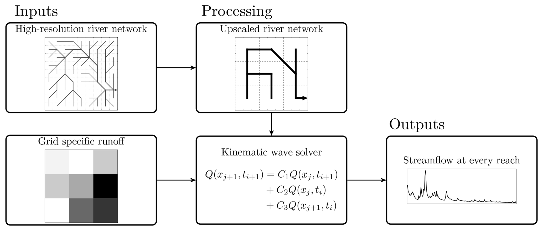
Figure 1 Flowchart of the processing steps required to run the multiscale routing model mRM. Left, inputs: static high-resolution information about the routing network and dynamic runoff field. Middle, internal mRM processing: aggregation of static and dynamic data to the routing resolution given by the user and execution of routing at this resolution. Right, output: calculated streamflow at prescribed gauge.

2.4 Data requirements and model setup

Three different input sources are required to run the multiscale routing model mRM. First, mRM requires information about the river network. mRM uses a rectangular grid to represent the river network over a domain (Yamazaki et al., 2011). Water can only be transported from a specific grid cell to one of the eight neighbouring cells following the steepest slope direction (D8 method, O'Calaghan and Mark, 1984). This procedure has to be carried at the highest possible resolution supported by the available dataset. For example, a high-resolution 100 m digital elevation model (DEM) can be used to calculate flow directions following the D8 method (Fig. 1 top left). It is worth mentioning that DEMs typically have to be adjusted to align with existing river networks using additional information about river locations (Döll and Lehner, 2002). High-resolution datasets such as HydroSHEDS (Lehner et al., 2008) can be used alternatively. Once the high-resolution flow direction is obtained following the nomenclature of the D8 method (2^d−1, $d=\mathrm{1},\mathrm{\dots },\mathrm{8}$; O'Calaghan and Mark, 1984), it is internally upscaled in mRM (Fig. 1 centre top) to the routing resolution specified by the user, employing the method of Döll and Lehner (2002). This upscaling technique has already been implemented in Samaniego et al. (2010). The flow direction in a low-resolution grid cell (3×3 grid in Fig. 1) is equal to the flow direction in the underlying high-resolution grid cell with the highest flow accumulation. If this high-resolution grid cell is not on an edge of the low-resolution grid cell, then the low-resolution grid cell is an outflow of the domain. It is worth mentioning that this procedure leads to incorrect basin areas at coarse resolution (Yamazaki et al., 2009). A detailed investigation of four large European river basins reveals that basin area is correctly calculated for model resolutions of less than 40 km (see Appendix C). At these resolutions, mRM will route water to the correct ocean basin in global-scale applications. Note that mRM can also handle rotated grids, if the high-resolution digital elevation model is provided on a rotated grid.

Second, the gridded runoff fields have to be provided in Network Common Data Form (NetCDF). Units of the forcing can be either millimetres per hour (mm h⁻¹) or kilogrammes per square metre per second (kg m⁻² s⁻¹) to facilitate applications to hydrologic models as well as land surface models. The most common use case is that mRM is applied to the sum of all runoff components of the driving model, which is based on the assumption that all components enter the river in the same grid cell. However, it is possible to apply mRM to different components individually which can be used as a model diagnostic. We acknowledge that Eq. (1) considers the entire channel flow. Its application to individual runoff components should be interpreted with caution, which may require conceptualisations for different flow celerities and varying topography among other factors. The spatial resolution of the runoff field is required to be a multiple of the resolution of the flow direction field. The most common use case is that streamflow is calculated at the resolution of the runoff, and mRM will upscale the river network to the routing resolution level as described before. However, mRM puts no constraints on model resolution. Simulations at higher or lower resolutions can be conducted as long as it is a multiple of both the runoff grid and the grid of the flow directions. In this case, runoff will be up- or downscaled employing weighted area fractions, which guarantee mass conservation. When mRM is coupled to coarse-scale simulations (e.g. spatial resolution of 1^∘), it is advisable to choose a lower resolution for mRM to correctly represent basin areas (see Appendix C).

Third, observed river streamflow can be provided to mRM at multiple locations within the river network. These locations have to be specified within the high-resolution river network and are then located on the upscaled river network internally within mRM. However, users should be cautious when selecting the model resolution so that the streams represented by the gauging data are still resolved within the upscaled river network. Thus, the upscaled flow accumulation in each grid cell is given in an output NetCDF file, which allows comparison to the drainage area of a given gauge. Observed discharge data are not required for mRM when applied, for example, at ungauged locations. They are, however, mandatory when performing model optimisation. Different error measures such as Nash–Sutcliffe efficiency (Nash and Sutcliffe, 1970) and Kling–Gupta efficiency (Gupta et al., 2009) can be calculated directly in mRM to inform the user about model performance.

A test basin is provided alongside the model code to illustrate the different data required to run the model and their formatting. The model code also contains pre-processing scripts to calculate the flow direction from a given DEM or flow accumulation from given flow directions.

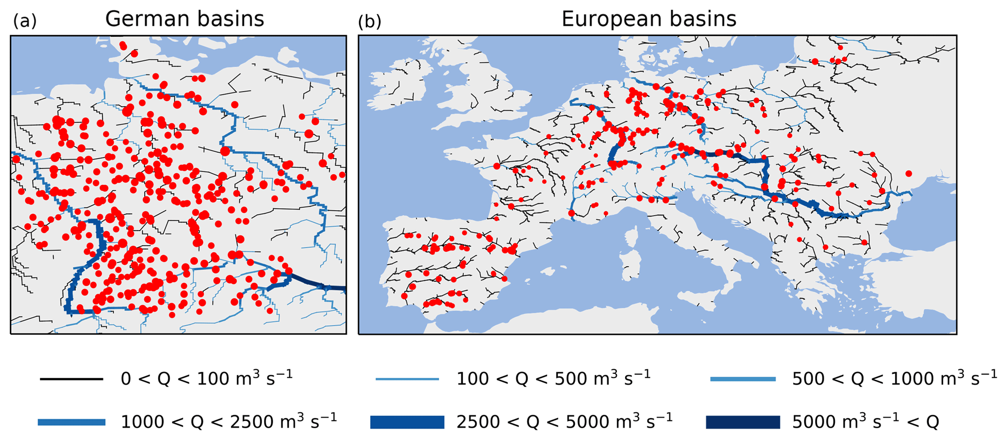
Figure 2 Discharge gauges used for the evaluation of the multiscale routing model mRM: (a) 368 gauges in the German dataset and (b) 254 gauges in the European dataset. In the background, the results of a pan-European simulation using the multiscale routing model mRM and the mesoscale hydrologic model mHM at a 5 km resolution are shown. The simulated streamflow Q is depicted for 5 August 2002.

2.5 Experimental setup

A total of 622 stream gauges are used in this study to assess the performance and scaling capabilities of mRM (Fig. 2). These contain 368 basins in the German dataset (Fig. 2a) and 254 basins in the European dataset (Fig. 2b). Input for mRM is derived from simulations carried out with the mesoscale hydrologic model mHM (Samaniego et al., 2010; Kumar et al., 2013b). Two different model setups for mHM are used in this study. The setup for the German dataset is identical to Samaniego et al. (2013) and Zink et al. (2016) with details given in Zink et al. (2017). The flow direction and accumulation are derived from a 100 m DEM. The setup for the European dataset was used in Thober et al. (2015) with details given in Rakovec et al. (2016). The DEM used to derive the river network has a 500 m resolution in this case. Runoff simulated by mHM was stored at hourly and daily resolutions in NetCDF files for both sets of basins. mHM simulations for the German dataset are provided at 4 km resolution while European simulations are provided at 24 km spatial resolution. The difference originates from the available meteorological forcing datasets, which are derived from station data of the German weather service at 4 km resolution (Zink et al., 2017) for the German dataset, while E-OBS data at 24 km resolution (Haylock et al., 2008) were used for the European dataset. To study the spatial scalability of mRM, streamflow is routed at different spatial resolutions, which are 1, 2, 4, 8, and 16 km for the German dataset and 3, 6, 12, 24, and 48 km for the European dataset. The selected resolutions cover a range of hydrologic applications from small- to large-scale modelling studies (Wood et al., 2011; Samaniego et al., 2017a) as well as scales of 0.5^∘ used in climate studies (Taylor et al., 2012; Jacob et al., 2014). Input runoff at 4 km for the German dataset and at 24 km for the European dataset is rescaled internally in mRM to the desired routing resolution that is provided in a configuration file.

The mesoscale hydrologic model mHM coupled to mRM using the regionalised Muskingum–Cunge (rMC) and the adaptive time step (aTS) parameterisation were calibrated at all catchments to provide a realistic representation of the hydrologic cycle. Details about model calibration can be found in Samaniego et al. (2010), Kumar et al. (2013b), Rakovec et al. (2016), and Zink et al. (2017). The calibrations of both mHM and mRM parameters are carried out using the shuffled complex evolution (SCE) algorithm (Duan et al., 1992). The SCE is coupled internally to both models, and SCE parameters (e.g. number of complexes) can be specified by users in a name list.

The Kling–Gupta efficiency (KGE) is selected as a metric for evaluating model performance (Gupta et al., 2009). The KGE is composed of three measures that relate simulated and observed streamflow. These are the ratio of simulated and observed mean values, the ratio of simulated and observed standard deviations, and the Pearson correlation coefficient. In comparison to the Nash–Sutcliffe efficiency (NSE, Nash and Sutcliffe, 1970), KGE provides a more balanced metric that is less sensitive than NSE to high streamflow values.

The model calibration and evaluation employs daily values of observed streamflow. The observed values are obtained from the Global Runoff Data Centre (GRDC) for the period from 1950 to 2010. Although mRM is run internally at higher temporal resolutions, the simulated streamflow is eventually aggregated to daily values for comparison to observations. Daily observed values are chosen here because the hydrologic cycle can be investigated in greater detail compared to monthly values commonly used with land surface models (e.g. Hagemann et al., 2009; Zhang et al., 2016).

3 Results

3.1 General model performance and parameter sensitivities

The adaptive time step parameterisation (aTS) in mRM contains one parameter representing the relationship between terrain slope and streamflow celerity (γ in Eq. 5). There is also an adjustable coefficient for the space weighting in the finite difference solver (ϵ in Eq. 2). The sensitivity of the aTS to ϵ and γ is explored here. The performance of simulated streamflow of the aTS appears to be in general very high and almost independent of the choice of ϵ and γ.

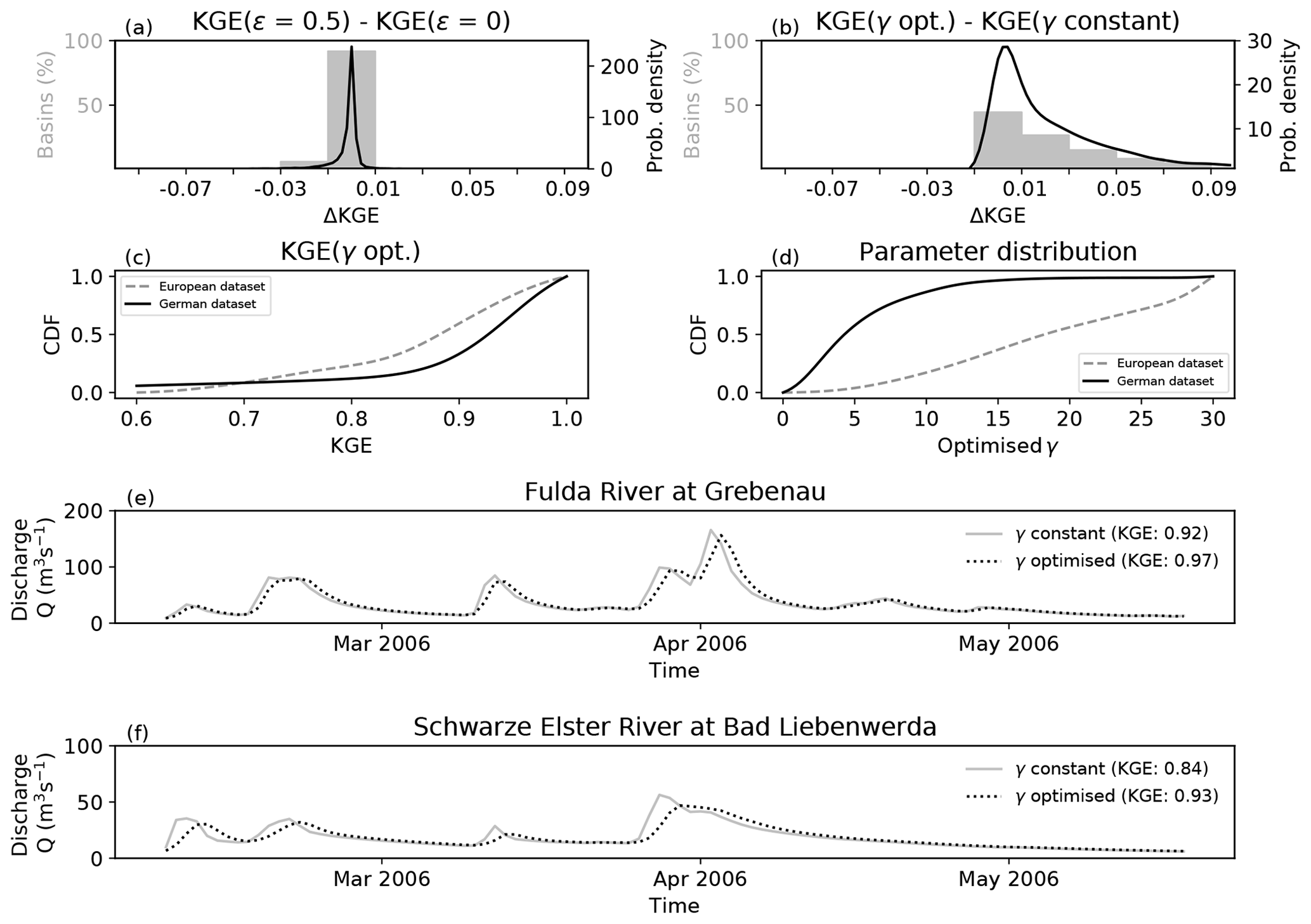
Figure 3 (a) Differences in KGE values between no numeric diffusion (ϵ=0.5) and full numeric diffusion (ϵ=0) for the combined European and German datasets, and
textbf(b) differences in KGE values between model runs with optimised parameter values at each gauge and one constant parameter for all gauges. Probability density functions (PDFs) are shown as black lines. The integrals of the PDFs over intervals of 0.02 (e.g. −0.01 to 0.01) are shown as grey bars normalised with respect to all basins. (c) Cumulative distribution functions (CDFs) of Kling–Gupta efficiencies (KGEs) for the European and German datasets separately based on optimised parameters γ. (d) CDFs of optimised γ for the two datasets. The underlying data shown in panels (a)–(d) are pooled for all catchments and all resolutions. Panels (e) and (f) show the hydrographs for two catchments at 4 km resolution for a parameter value of γ=15 (solid grey line) and the optimised value (dashed black line).

The density function peaks around ΔKGE=0 for the space-weighting factor ϵ (Fig. 3a). The ΔKGE estimated across the investigated basins is within the interval −0.03 to 0.01. All changes in KGE values below a magnitude of 0.01 are considered negligible, in alignment with previous literature, corresponding roughly to an error level in streamflow of 1 mm d⁻¹ (Kollat et al., 2012). Some large basins in the European dataset show up to 0.03 higher KGE values using ϵ=0 compared to ϵ=0.5. Note that the numerical diffusion of this finite difference solver (Eq. 4) depends linearly on ϵ (Cunge, 1969). An ϵ value of 0 corresponds to full numeric diffusion, whereas a value of 0.5 corresponds to no diffusion. The numerical diffusion is often chosen to correspond to the actual physical diffusion of the river by adjusting the value of ϵ (Todini, 2007; Beighley et al., 2009). The aTS is using a space-weighting factor ϵ=0 because this value provides slightly better estimates than a value of 0.5, but the impact of this factor is overall negligible.

The density function of ΔKGE is skewed when comparing the performances between optimised γ values at each gauging station and resolution with a constant value of 15 for all stations (Fig. 3b). A value of 15 is chosen because it provides the best compromise solution of the obtained optimised values (Fig. 3d). It can be expected that optimised parameters give higher performances than a fixed value. The performance increments with optimised parameters were, however, less than 0.01 in more than 37 % of the basins while only about 42 % of the basins exhibited ΔKGE values of 0.01 to 0.05. This means that performance increments with optimised γ values were below 0.05 in 79 % of the basins (Fig. 3b).

Overall, the KGE values for the European and German dataset are very high with only 4 % of the basins exhibiting a KGE value less than 0.6 (Fig. 3c). The median KGE values are 0.89 and 0.94 for the European and German dataset, respectively. KGE values are, however, highly dependent on the hydrologic model used (i.e. mHM) and the quality of the input data. The hydrologic model determines the partitioning of precipitation into evapotranspiration and runoff as well as the temporal dynamics of generated runoff. It thus affects all three components of the KGE: the bias, the variance, and the correlation. The routing model, on the other hand, is not able to change the long-term water balance, and is thus not affecting the bias term of the KGE. The routing model is, however, able to change the dynamics of simulated streamflow and thus greatly affects the variance term of the KGE. The distribution of the optimised parameter values is very different for the German and the European datasets with median values of 4 and 21, respectively (Fig. 3d). These differences originate from the resolution of the underlying digital elevation model (DEM) and hence the slopes used in Eq. (5). The slope data for the German dataset are available at a 100 m resolution, while it is at 500 m resolution for the European dataset. The slopes will be larger and more variable at 100 m resolution compared to 500 m resolution. This implies that lower slope values (European dataset) are associated with higher γ values, and higher slope values (German dataset) are associated with lower γ values, which results in similar celerities for the two datasets. This highlights that the parameter values obtained are highly dependent on the underlying dataset, which has been identified as a major source of hydrologic modelling uncertainty (Livneh et al., 2015).

Hydrographs for two German river basins that exhibit ΔKGEs of 0.05 and 0.11, respectively, are shown in Fig. 3e and f. These ΔKGE values were among the highest of all basins and model resolutions considered in this study. A shift in peak flows of about 1 d can be spotted visually at ΔKGE values of 0.05 (Fig. 3e). This difference is representative for around 21 % of all catchments. A difference in KGE of 0.11 implies a change in the amount and timing of peak flows (Fig. 3f) and is representative for around 8 % of all catchments. The overall recession dynamics are comparable independent of the change in γ (Fig. 3e and f). Moreover, no substantial shift in amount and timing of peak flows is observed in 79 % of the catchments. It will ultimately depend on the preference of the model user if parameter calibration is applied for a specific use case.

3.2 Temporal and spatial scalability

The aTS scheme is first run with different temporally aggregated inputs and second on different spatial resolutions to demonstrate its scalability across time and space.

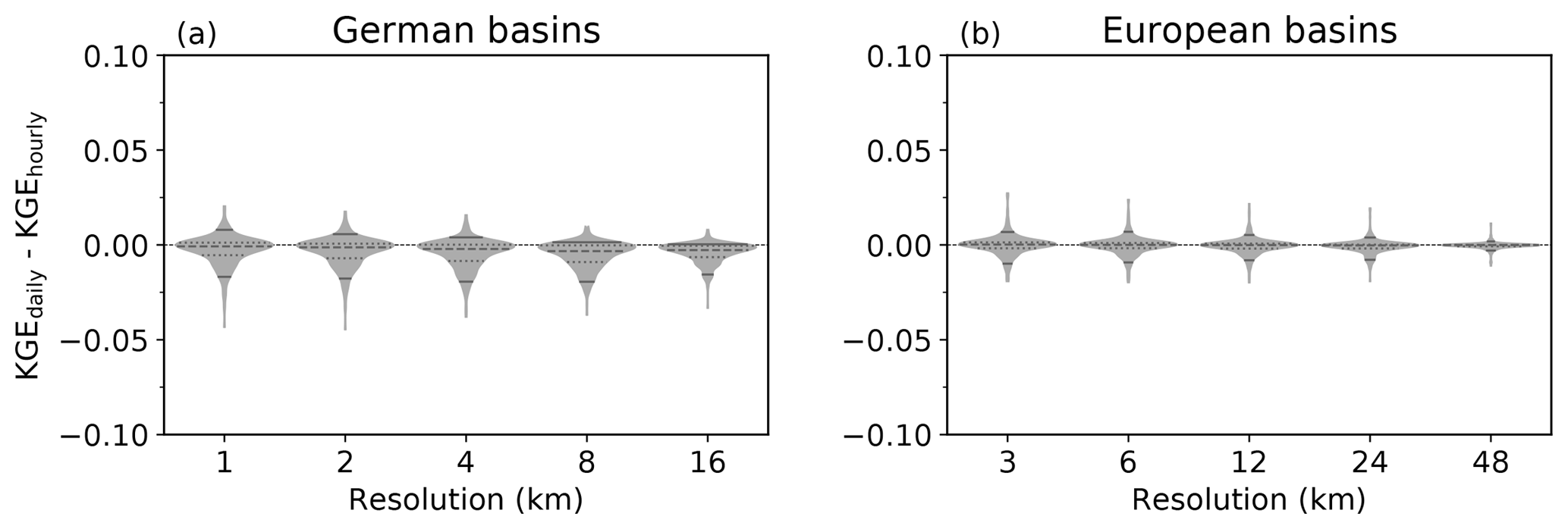
Figure 4 Probability density functions (PDFs) of differences in KGE values obtained with an hourly and daily input to the aTS. PDFs are limited to the minimum and maximum ΔKGE values and have been normalised with respect to its width to ease the comparison. A thin dashed horizontal line is given at ΔKGE=0 for reference. Dashed lines in the violins indicate the medians, dotted lines the 25th and 75th percentiles, and solid lines the 5th and 95th percentiles.

The adaptive time step procedure of the aTS allows the user to choose different input time steps. This might be the case if input runoff is provided as an aggregate over a specific period, for example as daily runoff. The aTS aggregates or disaggregates any given temporal resolution to the internal time step constrained by a Courant number of 1 (Eq. 6). Similar performances are achieved with the aTS using either daily or hourly inputs across all basins in the German and European dataset at every spatial resolution (Fig. 4). This is achieved by aggregation and disaggregation to the internal time step, but it is also affected by the fact that we compare against the observed daily discharge. Sub-daily differences are thus averaged out before comparison. Observed hourly discharge would contain information about sub-daily variability that could not be obtained from daily inputs and, thus, hourly inputs might perform better in this case. However, observed discharge is mainly available on a daily resolution.

Evidently, aggregated input provides less variable runoff to the routing scheme, leading to less variable river discharge. Aggregation does, however, not change the absolute values (bias). The ΔKGE values therefore appear due to changes in streamflow variability, which should be reduced with aggregated runoff values.

Subtle differences exist between the ΔKGE values for the German and European dataset. The median ΔKGE values are almost zero for the European basins (Fig. 4b) with very low standard deviations. Median ΔKGE values for the German dataset are in contrast slightly negative around −0.005 (Fig. 4a). The differences between the German and European dataset come mainly from the spatial resolution at which gridded runoff inputs for mRM were generated. Forcing for mRM was provided at 4 km resolution for the German dataset, which is the lowest resolution of the meteorological input (Zink et al., 2017). The input runoff for mRM has been generated at a 24 km resolution for the European dataset, which corresponds to the resolution of the meteorological E-OBS dataset (Haylock et al., 2008). Runoff data at the 4 km scale exhibit much higher spatial variability compared to the coarser 24 km runoff. The higher spatial variability of the German dataset is substantially reduced when using daily runoff compared to hourly runoff, which generates the small mismatch between using hourly and daily inputs for the German dataset (Fig. 4a). The equalisation of variability from averaging is less pronounced in the less variable runoff fields of the European dataset.

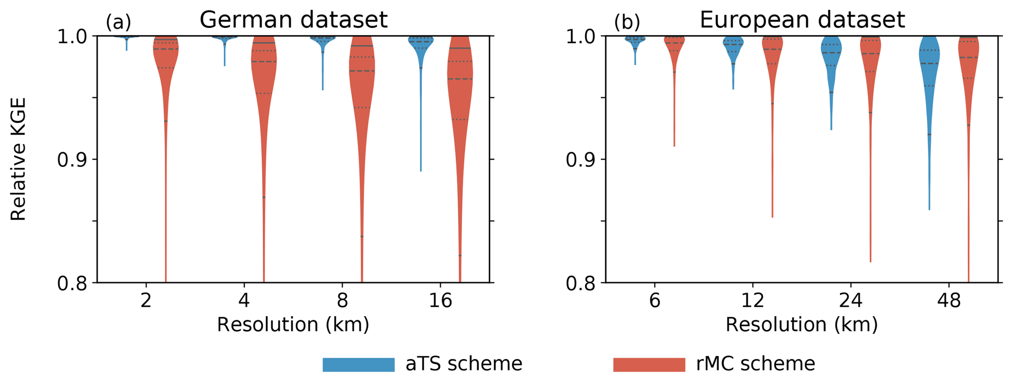
Figure 5 Probability density functions (PDFs) of relative KGE values for the adaptive time step scheme (aTS, blue violins) and the regionalised Muskingum–Cunge (rMC) routing scheme (red violins). KGE values are calculated relative to the finest possible spatial resolution, which is 1 km for the German (a) and 3 km for the European dataset (b). PDFs are limited to the minimum and maximum relative KGE values and are scaled to the same widths. Dashed lines in the violins indicate the medians, dotted lines the 25th and 75th percentiles, and solid lines the 5th and 95th percentiles.

For the spatial scaling, KGE values relative to the finest possible model resolutions (1 km for German and 3 km for European dataset) are reported (Fig. 5). In other words, the reference values (observations) in the calculations of KGE are replaced by simulated streamflow obtained with optimised parameters at the highest resolution. Perfect spatial scaling is hence indicated by a relative KGE value of 1. Figure 5 shows the probability density functions of the relative KGE values estimated over all basins for each model resolution. The optimised parameter obtained at the highest spatial resolution for each basin is transferred for the aTS and the rMC parameterisation to the model runs at the coarser spatial resolutions.

Results shown in Fig. 5 clearly demonstrate a remarkable spatial scalability of the aTS in comparison to the original rMC parameterisation. The lowest median relative KGE of 0.977, which represents a change of less than 3 %, is observed at the coarsest resolution of 48 km for the European dataset. The overall lowest relative KGE is 0.85 for the aTS and 0.22 for the rMC scheme. The aTS scheme shows an improved scalability because it considers the between-grid heterogeneity of celerities through the parameterisation based on terrain slope (Eq. 5) and the numerical stability criteria (Eq. 6). The spatial scalability of the aTS is higher for the German dataset compared to the European dataset. This can be attributed to the spatial resolution of the slope data used in the parameterisation of celerity (Eq. 5), which is available at 100 m resolution in the German dataset compared to 500 m in the European dataset. The representation of river slopes is thus more realistic in the German dataset. Notably, a similar spatial scalability is found for both the aTS and rMC parameterisation if default parameters are used (not shown).

The adaptive time step scheme (aTS) shows, in summary, remarkable temporal and spatial scalability in comparison to its predecessor. The adaptive time step allows for aggregated or disaggregated input (generated runoff) from any given temporal resolution.

3.3 Comparison of adaptive time step routing with regionalised Muskingum–Cunge parameterisation

The adaptive time step scheme (aTS) is the successor of the regionalised Muskingum–Cunge (rMC) routing implemented in mHM. A detailed analysis of the differences in model performances between the two routing parameterisations is presented here for the German and European dataset and selected spatial resolutions (Fig. 6).

Figure 6 Differences in KGE between the multiscale routing model mRM using a optimised parameter γ, constant parameter value γ=15, and the original Muskingum–Cunge routing scheme (rMC) implemented in the mesoscale hydrologic model mHM for the German (left column) and European datasets (right column). The ΔKGE values between the aTS and rMC using optimised parameter values on each basin and at each resolution are shown for the respective basins on the left of each panel; basins are sorted according to catchment area (note the logarithmic scale). Cumulative distribution functions of ΔKGE between the aTS and rMC using optimised parameter values (solid blue line) and the aTS with a constant parameter, and rMC with optimised ones (dashed red line) are depicted on the right of each panel. The line at KGE = 0 (dashed black line) is added for reference.

The performances are comparable across the German and European dataset (Fig. 6) if the aTS and rMC are calibrated individually on each basin and at each resolution. However, the cumulative distribution functions (CDFS) of ΔKGE values are skewed towards positive values indicating, in general, higher performance for the aTS than rMC (Fig. 6a–j, solid blue line in right panels). This improvement is slightly higher for the German dataset compared to the European, which can be attributed to the higher spatial resolution of the slope data in the former. The ΔKGE values are closer to zero for resolutions finer than 4 km, indicating a more comparable model performance for the aTS and rMC at higher spatial resolutions than at coarser ones. This is due to the fact that the original rMC routing scheme was developed at this resolution (Samaniego et al., 2010; Kumar et al., 2013b). At spatial resolution coarser than 12 km, the rMC routing strongly violates the Courant–Friedrichs–Lewy criterion (i.e. $c\mathrm{\Delta }t/\mathrm{\Delta }x\le \mathrm{1}$) and results in poorer performance. Even re-optimising the routing parameters cannot compensate for the scaling error because water is moved too fast through the river network. At these coarse resolutions, the aTS scheme is still outperforming the rMC scheme when run with a constant γ=15 parameter for all catchments (Fig. 6a–j, dashed red line in right panels).

In summary, the adaptive time step scheme (aTS) demonstrates at least the same performances as its calibrated predecessor, the regionalised Muskingum–Cunge routing scheme (rMC). The scalability of mHM across spatial resolutions has been demonstrated before, but employing a fixed spatial routing resolution for the rMC scheme (see Kumar et al., 2013a). For this purpose, the gridded runoff fields are spatially up- or downscaled to the specified spatial resolution (e.g. 8 km runoff field disaggregated to 4 km). The aTS parameterisation allows the user to simultaneously scale both the hydrologic and routing model. Notably, the aTS requires no specific up- or downscaling of runoff fields, and parameters can be transferred across spatial and temporal resolutions. Both of these properties offer distinct advantages in reducing the computational costs because mRM can be directly applied at the resolution of the gridded runoff input. Using a constant γ=15 parameter for all catchments, avoiding optimisation, further reduces the computational costs but might result in slightly decreased model performances in comparison to model runs with optimised γ values (ΔKGE≈0.1 at a 95 % confidence interval). This is, however, still small compared to the impact that the hydrologic model used as input to the routing scheme has. Using fixed γ parameters also enable the seamless application of the aTS at ungauged basins (Rakovec et al., 2016).

3.4 Streamflow simulations over the Danube catchment by applying mRM to the regional climate model REMO

Regional climate models (RCMs) are used to dynamically downscale global climate models over a specific region to obtain higher-resolution information about the local climate. The evaluation of RCMs often focuses on surface fluxes and states such as 2 m air temperature, precipitation, and evapotranspiration amongst others. River runoff, which provides an integrated signal of the water cycle over a region, is not often used as a further model diagnostic. This might be, besides other reasons, due to the fact that RCMs are designed to be run at various spatial resolutions, ranging from few kilometres (e.g. Jacob et al., 2014) to tenth of kilometres (e.g. Van der Linden and Mitchell, 2009). Hence RCM output has to be aggregated or disaggregated to current routing schemes with fixed routing resolutions. This is not necessary with the multiscale routing model mRM employing the adaptive time step parameterisation (aTS) that runs seamlessly at various spatial and temporal scales (Sect. 3.2). This eases the comparison of RCM-derived streamflow with observations as the routing model has to be set up only once and can then be applied at different resolutions without adjusting the model parameter γ or the model setup.

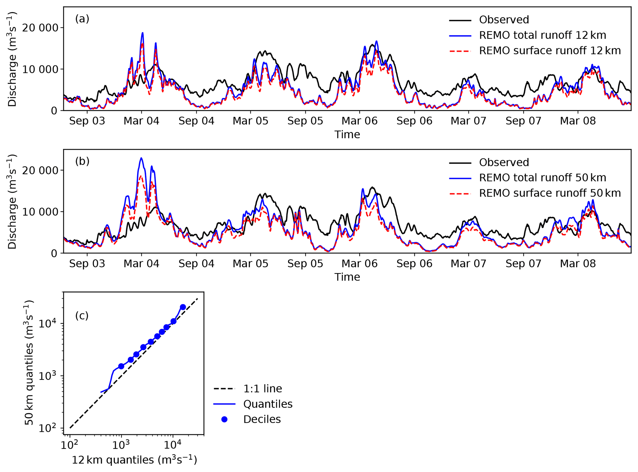
Figure 7 Hydrographs for the Danube basin at the gauging station Ceatal Izmail. Hydrographs were obtained by routing runoff output from the regional climate model REMO with mRM, employing the adaptive time step parameterisation (aTS) at spatial resolutions of 12 km (a) and 50 km (b). The solid black line shows the observed streamflow. The solid blue line is mRM output using the sum of the REMO surface and subsurface runoff components as input. The dashed red line is mRM output using only the REMO's surface runoff component. Panel (c) quantile–quantile plot of the routed REMO outputs (sum of surface and sub-surface components) at 12 and 50 km resolutions.

This section shows one exemplary application of mRM to the output of the regional climate model REMO (Jacob et al., 2001) over the Danube catchment. Generated runoff by REMO has been obtained from the EURO-CORDEX project (Jacob et al., 2014) at 12 and 50 km resolutions. Both resolutions were used to run mRM employing the aTS parameterisation (γ=15) over the Danube catchment (Fig. 7a for 12 km and b for 50 km). REMO was nested into ERA-Interim reanalysis in the EURO-CORDEX project, which therefore permits the comparison with observed streamflow. The Danube basin is part of the European dataset used for the evaluation in previous sections. The same setup was used for routing gridded runoff fields of the REMO model, and only the number indicating the routing resolution had to be changed in the mRM configuration file.

There are striking differences between the observed and simulated streamflow (Fig. 7). This is due to the fact that REMO uses a simple runoff generation consisting of direct surface runoff and soil drainage. There is no groundwater description in REMO so that the only water storage is in the river itself, and the baseflow is much too low. This becomes evident as most runoff generated by REMO is surface runoff. REMO at 50 km resolution shows substantial contribution from sub-surface runoff only during spring 2004 (Fig. 7b). This highlights a common misunderstanding when using river routing with land surface models: most land surface models include only a simple runoff generation that does not account for the temporal variability of the runoff signal, which is separated into fast flow, interflow and baseflow in hydrologic models (e.g. mHM). Routing directly drainage fluxes leads to seasonal high flows that are much earlier than observed. Using very low celerities in the routing models might improve this model–data mismatch (see Oki et al., 1999, for celerities in several routing schemes). Other runoff schemes represent different runoff components within the model code (e.g. Lohmann et al., 1996; Hagemann and Dümenil, 1997; Pappenberger et al., 2009). The multiscale routing model mRM does not contain runoff generation because most hydrologic models already include detailed runoff generation, and nowadays land surface models also start to include groundwater components (e.g. Niu et al., 2011; Clark et al., 2015). Details of these components depend strongly on model focus which should not be imposed by the river routing model (cf. Sect. 4).

Three main conclusions can be drawn from the comparison of modelled and observed discharge. First, REMO is able to capture the overall seasonal variations of runoff. There is a pronounced seasonality within the first 3 years in both observations and the REMO simulated streamflow, which is much reduced in the last 2 years (Fig. 7a and b). Seasonality in the Danube catchment is dominated by spring melt, which is very low in the last 2 years. REMO is therefore able to simulate inter-annual variations in precipitation and surface temperature over the Danube catchment.

Second, REMO produces too little runoff on average at both resolutions. Runoff is underestimated by about 30 % and 17 % at 12 and 50 km resolutions, respectively. Interestingly, REMO overestimates catchment average precipitation compared to E-OBS (Haylock et al., 2008) by 2 % and 15 % on 12 and 50 km, respectively. Hence, the partitioning of precipitation into runoff and evapotranspiration is not correct in REMO, under the reasonable assumption that groundwater tables around the Danube exhibit no significant trend over the simulation period. This implies that evapotranspiration is overestimated very similarly on 12 and on 50 km resolution by REMO.

Third, REMO exhibits statistically different runoff on both model resolutions (i.e. 12 and 50 km). The quantile–quantile plot (Fig. 7c) shows that the 50 km simulation produces more runoff than the 12 km simulation, most likely because REMO simulates also higher precipitation at 12 km resolution. It is worth noting that this mismatch is not present in the ENSEMBLES project (see Appendix D).

This section underlines the fact that hydrologic and land surface models have to include the processes of runoff generation and groundwater for a fair comparison of modelled and observed streamflow. Process parameterisations with an instantaneous surface runoff component are common in land surface models (LSMs,Vereecken et al., 2019), but they are too inflexible to reproduce the observed discharge. After the augmentation of LSMs with these process parameterisations, which account for more runoff components (e.g. fast and slow interflow), the multiscale routing model mRM would allow the further analysis of the responses of land surface models to climatic extremes (Reichstein et al., 2013) using indices and signatures of the discharge time series (Thober and Samaniego, 2014; Shafii and Tolson, 2015).

4 Comparison with existing routing schemes

River routing is performed at various resolutions depending on the application. Global streamflow simulations, using output of land surface models (LSMs) or hydrologic models (HMs) for example, are typically carried out at 0.5^∘ or 1.0^∘ resolutions (among others, Oki et al., 1999; Hagemann et al., 2009; Pappenberger et al., 2009; Zhang et al., 2016). However, climate models are run on ever increasing spatial scales (Jacob et al., 2014), or using even internally nested grids or zooming functionality (Zängl et al., 2014). Also, spatial resolutions of few kilometres are used within the hydrologic modelling community to obtain national and continental estimates of hydrologic fluxes and states (David et al., 2011; Marx et al., 2018; Thober et al., 2018; Wanders et al., 2019). Despite the fact that diverse spatial resolutions are used to represent the hydrologic cycle, spatial resolutions of routing are mostly fixed and cannot be changed easily. In many models, the user needs to provide the input data (e.g. flow direction, DEM, and channel information) for every resolution that the model is applied to (among others, Lohmann et al., 1998; Beighley et al., 2011; Neal et al., 2012). The multiscale routing model mRM, on the other hand, is able to scale the river network to the desired routing resolution internally. This allows the full use of the information provided by the input runoff data, without uncertainties coming from the rescaling process (e.g. from a 12 km LSM output to a 0.5^∘ river network). It also avoids scaling the input runoff to a hyper-resolution river network, which then requires high-performance computing resources such as in the case of the RAPID framework (David et al., 2011). This might especially be valuable if parameter estimations using discharge data need to be carried out, which require a large amount of model evaluations.

Current solvers describing water movement within a river network can in principle be applied at different resolutions. For example, the solution of the diffusion equation by Green's function proposed by Lohmann et al. (1996) is valid independently of the resolution of the river network. The CaMa-Flood model can similarly be applied to different resolutions as long as the Courant–Friedrichs–Lewy condition is fulfilled (Yamazaki et al., 2013). The aTS employs the same condition to identify an adaptive time step that guarantees the numerical stability and achieves a scalability across spatial resolution. Yamazaki et al. (2009) also developed a pre-processor for the CaMa-Flood model that explicitly allows the generation of a river network at different spatial resolutions. mRM follows the same idea but it internally includes the upscaling of the river network to the required resolution in the model code. The user has to provide the routing network only once even if the application will focus on different spatial resolutions. The derived river network can be stored in a restart file to further speed up the computation (see Appendix B for run times). However, the aTS performance is dependent on the resolution of the underlying slope data (see Sect. 3.1 and 3.2), and it is advisable to use the highest-resolution data available. This is due to the fact that channel slope instead of terrain slope should be used in Eq. (5) and a high-resolution DEM provides a close approximation of channel slope.

Another reason that the scalability of existing routing models is hampered is that they include not only the routing of water in the river network but also a runoff generation mechanism, which represents a variety of other components of the hydrologic cycle (Pappenberger et al., 2009). The complexity of existing runoff generation descriptions reflects the diversity of use cases of hydrologic and land surface models. Descriptions range from simple linear models (Niu et al., 2011; Beven, 2012) to more complex representations considering surface groundwater interactions (Maxwell and Kollet, 2008; Miguez Macho and Fan, 2012). Existing routing schemes often opt for more simple parsimonious representations. For example, routing models use linear reservoirs for overland flow, baseflow, and river flow to delay runoff generated by the land surface (e.g. Hagemann and Dümenil, 1997; Pappenberger et al., 2009; Getirana et al., 2012). The mRM does not include any runoff generation because it is beyond the scope of a river routing model to reflect the complexity of existing runoff generation processes. Notably, there is currently ongoing research into understanding how a particular process parameterisation impacts hydrologic simulations (Niu et al., 2011; Clark et al., 2015). Runoff generation also hampers the scalability of routing models because of their highly non-linear behaviour. The multiscale parameter regionalisation (MPR, Samaniego et al., 2010) is one of few approaches that has proven to provide consistent generated runoff at resolutions ranging from 2 to 16 km for mesoscale catchments (Kumar et al., 2013b) and from 0.125 to 1^∘ for continental-scale basins (Kumar et al., 2013a).

Among the plethora of routing models presented over the past decades, only few have rigorously evaluated their spatial scalability. The “Model for Scale Adaptive River Transport” (MOSART) has been developed explicitly to achieve seamless application of river routing across scales (Li et al., 2013) similar to mRM. MOSART has been successfully coupled, for example, to the Community Land Model to compare with global discharge data (Li et al., 2015). MOSART differs from mRM by solving the kinematic wave equation with Manning's equation for channel velocity (Manning, 1891) not only for the main channel but also for hillslope routing and sub-grid tributaries. It thus explicitly accounts for sub-grid heterogeneity by considering all lateral travel times across hillslopes and tributaries. The mRM, on the other hand, solves a kinematic wave equation with spatially varying velocities for the main channel only (Eqs. 1 and 5). The assumption within mRM is that travel times in the main channel dominate travel times at hill slopes and tributaries, and the latter are negligible. This, in turn, leads to a simpler approach with one model parameter. However, further research is needed to explicitly investigate the validity of this model assumption. It is for example possible to return to the original formulation of Miller et al. (1994), using a reference slope s₀ that should depend on the underlying digital elevation model (DEM). But two DEM resolutions, as in this study, are not enough to find a suitable formulation for the dependence of s₀ on DEM characteristics such as resolution or maximal slope. Hence s₀ was lumped with the minimum celerity c₀ to give only one identifiable parameter γ.

It is worth remembering that mRM represents a simple approach towards river routing. The results in this study demonstrate that mRM employing the adaptive time step parameterisation in combination with upscaled high-resolution celerities (aTS) achieve almost identical daily streamflow simulations at various model resolutions in diverse German and European catchments. Recent literature has shown that a realistic representation of streamflow in river basins with extensive floodplains such as the Amazonas, Niger, and Congo rivers require the representation of floodplain inundation processes (Getirana et al., 2012; Paiva et al., 2013; Fleischmann et al., 2016; Pontes et al., 2017). Floodplain processes are currently not considered in mRM, and further research is required to include these. Paiva et al. (2013) showed that floodplain processes dominate the difference between hydrodynamic and kinematic wave models. The approach used therein should be exploited within the mRM to be applicable at different resolutions.

5 Conclusions

The adaptive time step scheme in combination with upscaled high-resolution celerities (aTS) implemented in the multiscale routing model mRM estimates streamflow at various resolutions ranging from the hyper-resolution of 1 km to the large scale of 0.5^∘. Differences in Kling–Gupta efficiencies of simulated daily streamflow between various model resolutions and temporal forcings are negligible with a median of 0.03 over Germany and Europe (Sect. 3.2). The aTS scheme shows an improved scalability over its predecessor because it considers the linkage between spatial resolution and integration time step by virtue of the Courant criteria (Eq. 6). It considers the between-grid heterogeneity of celerities through the parameterisation based on high-resolution terrain slope (Eq. 5). mRM represents the river network internally at the resolution of the model input, which allows seamless application to output of any hydrologic model (HM) and land surface model (LSM). It can also easily be coupled internally in the code of HMs or LSMs, providing error measures such as Nash–Sutcliffe and Kling–Gupta efficiencies for model evaluation or calibration.

The mRM uses a simple kinematic wave equation to describe water flow within a river network. This representation is regarded suitable as long as backwater effects and floodplain inundation processes are comparatively small. The mRM does not represent runoff generation mechanisms, which are included in other routing models. Runoff generation is included in hydrologic models and nowadays often in land surface models. The details of the implementation depend strongly on the application of interest. Users of river routing schemes should not be limited by the options implemented in the river routing model itself.

The mRM can in principle be used on rotated model grids commonly used for climate models if high-resolution flow directions are provided at the same grid. However, mRM represents the river network as a rectangular grid, allowing the application of a constant time step over the entire model domain. Future developments will focus on implementing reservoirs and natural lakes, floodplain processes, and a location-dependent time stepping scheme. The latter will enable the use of mRM on irregular grids or in models with local refinement. Also, parallelisation is currently implemented in mRM to take full advantage of high-performance computing clusters. The model source code along with a test case to validate successful installation is freely available within the codebase of the mesoscale hydrologic model (mHM) at http://www.ufz.de/mhm (last access: 21 June 2019).

Appendix A: Regionalised Muskingum–Cunge (rMC) routing

The regionalised Muskingum–Cunge (rMC) parameterisation implemented in the mesoscale hydrologic model (mHM) calculates the Muskingum coefficients C₁, C₂, and C₃ in Eq. (3) as a function of high-resolution river network properties. The coefficients C₁, C₂, and C₃ are parameterised as follows:

$$\begin{array}{}\text{(A1)}& C_{\mathrm{1}}={\mathit{\nu }}_{\mathrm{2}};C_{\mathrm{2}}={\mathit{\nu }}_{\mathrm{1}}-{\mathit{\nu }}_{\mathrm{2}};C_{\mathrm{3}}=\mathrm{1}-{\mathit{\nu }}_{\mathrm{1}},\end{array}$$

where the parameters ν₁ and ν₂ are given as

$$\begin{array}{ll}{\displaystyle }& {\displaystyle }{\mathit{\nu }}_{\mathrm{1}}={\displaystyle \frac{\mathrm{\Delta }t}{\mathit{\beta }(\mathrm{1}-\mathit{ϵ})+\frac{\mathrm{\Delta }t}{\mathrm{2}}}},\\ \text{(A2)}& {\displaystyle }& {\displaystyle }{\mathit{\nu }}_{\mathrm{2}}={\displaystyle \frac{\frac{\mathrm{\Delta }t}{\mathrm{2}}-\mathit{\beta }\mathit{ϵ}}{\mathit{\beta }(\mathrm{1}-\mathit{ϵ})+\frac{\mathrm{\Delta }t}{\mathrm{2}}}},\end{array}$$

following the nomenclature of Appendix A2 in Samaniego et al. (2010). This formulation is identical to Eq. (4) of the present study, using $\mathit{\beta }=\mathrm{\Delta }x/c$ in Eq. (A2) and substituting Eq. (A2) into Eq. (A1). The parameters β and ϵ are then conceptualised as

$$\begin{array}{ll}{\displaystyle }& {\displaystyle }\mathit{\beta }={\mathit{\gamma }}_{\mathrm{1}}+{\mathit{\gamma }}_{\mathrm{2}}L+{\mathit{\gamma }}_{\mathrm{3}}S+{\mathit{\gamma }}_{\mathrm{4}}C,\\ \text{(A3)}& {\displaystyle }& {\displaystyle }\mathit{ϵ}={\mathit{\gamma }}_{\mathrm{5}}{\displaystyle \frac{S}{max\left(S\right)}},\end{array}$$

where L is the length of the reach, S is the slope of the reach, and C is the fraction of impervious land cover within the floodplains (see Table 4 in Kumar et al., 2013b). Overall, there are five global parameters, γ₁ to γ₅, in Eq. (A3) that can be chosen by the user. The integration time step is fixed at 1 h. To guarantee the numerical stability of the parameterisation, the following upper and lower bounds are applied:

$$\begin{array}{}\text{(A4)}& {\displaystyle }& {\displaystyle }\mathrm{0}<\mathit{ϵ}\le \mathrm{0.5},\text{(A5)}& {\displaystyle }& {\displaystyle \frac{\mathrm{\Delta }t}{\mathrm{2}(\mathrm{1}-\mathit{ϵ})}}<\mathit{\beta }\le {\displaystyle \frac{\mathrm{\Delta }t}{\mathrm{2}\mathit{ϵ}}},\end{array}$$

where Δt is set to 1 h.

Appendix B: Run times

The run times of mRM do not scale linearly with the number of grid cells. The reason is that the arrays containing the network information cannot be stored continuously in the memory because the river network can be mathematically represented as a tree. The run times for a small and large basin are reported here to provide an overview of the range of possible run times. The Moselle catchment, with an area of 28 286 km², is selected to represent a small catchment. A spatial resolution of 24 km results in 34 grid cells to cover the Moselle catchment. The river Danube with an area of 801 463 km² is selected to represent a large catchment. The REMO simulations (Sect. 3.4) at 12 km resolution resulted in 5775 grid cells.

The run time has to be separated for the initialisation and computation step of mRM. During the initialisation step of mRM, all input data are read and the high-resolution river network is upscaled to the model resolution specified by the user. mRM offers restart capabilities that allows the user to perform this step only once. The initialisation of mRM takes about 1.3 and 3300 s for the Moselle and Danube rivers, respectively. It heavily depends on the speed of I/O because all the data are read during this step and the cache size of the employed CPU might limit the execution time. If mRM reads the upscaled river network from a restart file, this step will take a negligible amount of time. For example, the initialisation step takes 60 s for the river Danube if a restart file is used. During the computation step of mRM, the streamflow values within the river network are calculated. The run time of this step scales linearly with the length of the simulation period. This step takes 0.1 and 24 s per year for the Moselle and Danube rivers, respectively. These run times have been estimated with the Intel 18 Fortran Compiler and level 3 code optimisation on a Dual Intel Xeon Platinum 8169 CPU (http://www.fz-juelich.de/ias/jsc/EN/Expertise/Supercomputers/JUWELS/Configuration/Configuration_node.html, last access: 21 June 2019).

Appendix C: Drainage area for different model resolutions

The D8 method (O'Calaghan and Mark, 1984) is known to be unable to reproduce the basin area correctly at large scales (e.g. 1^∘). This effect can also be seen for mRM in four major European river basins (Fig. C1). The setup for this analysis is the same as the one described in Samaniego et al. (2018, see data availability section). Two use cases of mRM are investigated here: first, a single-basin setup where the entire model domain drains to one outlet; second, a continental-scale setup that contains multiple rivers, and the model domain contains multiple outlets. In the former case, the basin area calculated in mRM is independent of the model resolution and equal to the basin area at the high-resolution input data (0.5 km in this case). This is achieved by using weighted area fractions for grid cells that are only partly covered by the study domain. The calculated basin area is very close to the true basin area and differences stem from mismatches in the delineation of the basin. In the second case, the basin area is correctly reproduced up to a model resolution of 40 km and tends to increase for lower-resolution models (blue markers in Fig. C1). This effect is larger for small basins (e.g. the river Elbe and the river Loire) than for large basins (e.g. the river Danube) because it enlarges as the ratio between basin size and model resolution decreases. The increase of basin area with the size of grid cells can be expected because larger grid cells have longer edges and thus unify more head water streams. If the underlying rivers do not unite, but depart downstream, then water is not routed correctly and no meaningful analysis can be carried out. Yamazaki et al. (2009) provide an insightful illustration of this deficiency in the D8 method at the 1^∘ resolution. They also proposed an improvement of the D8 method to correctly route water at this coarse scale and provide an example for the Mekong, Salween, and Yangtze rivers (see Fig. 6 in Yamazaki et al., 2009). This improvement is not implemented in mRM because firstly the basin area is correctly represented in single-site setups, which are frequently used for parameter estimation. Secondly, mRM can be run at high resolution of less than 40 km even if the input is provided at coarser scale (e.g. 100 km). The mRM distributes the input equally among all high-resolution grid cells and then routes the water downstream. The mRM is also computationally efficient to simulate streamflow at a high resolution of 5 km over continental scales in the context of climate change studies (e.g. Thober et al., 2018; Marx et al., 2018) and seasonal forecasting (Wanders et al., 2019). Notably, the calculated flow accumulation of mRM is saved in a restart file. The user can thus easily check whether the chosen model resolution adequately represents the actual river basin size (i.e. within the acceptable error bounds).

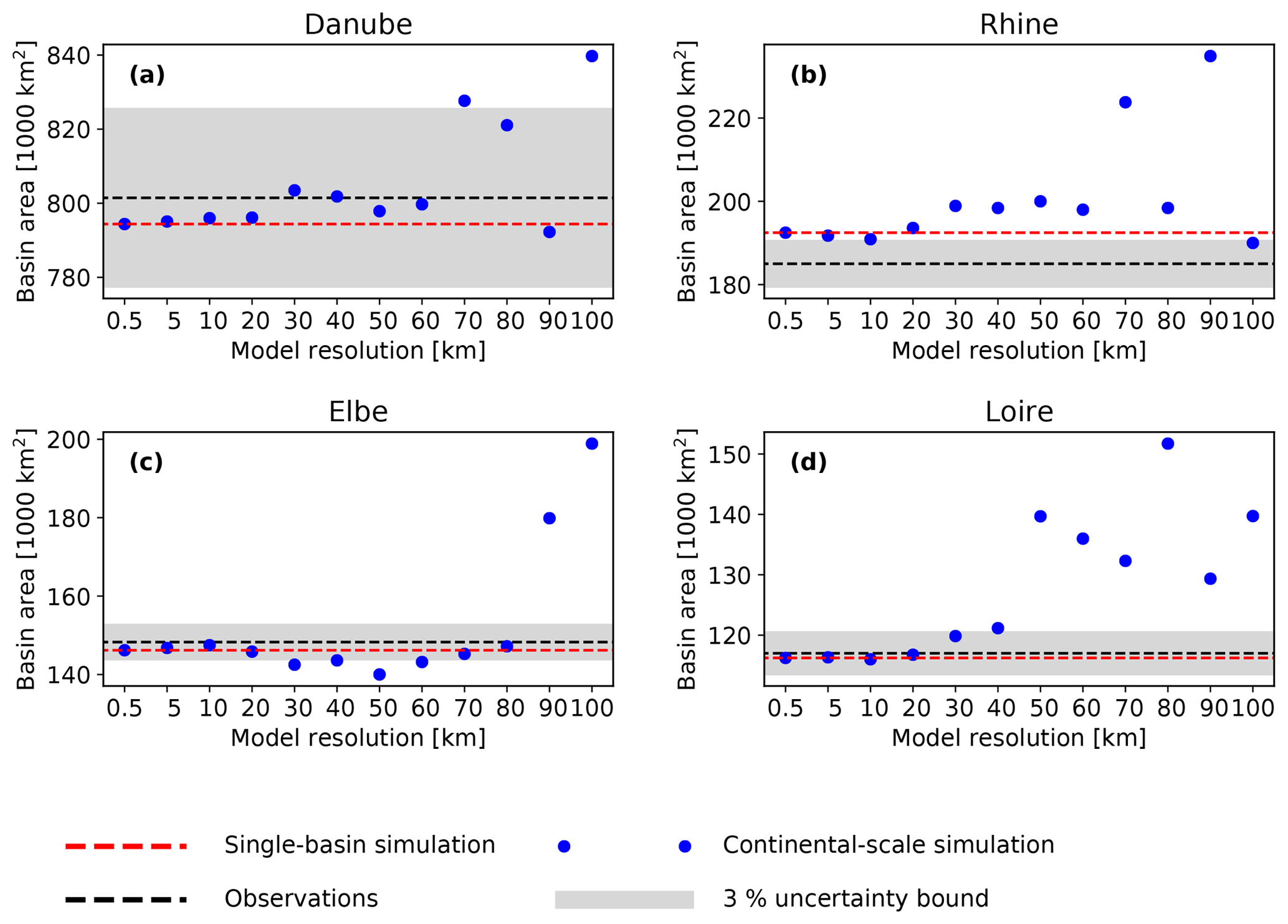
Figure C1 Basin areas for four major European river basins. Blue circles denote the calculated basin area derived by the D8 method at different resolutions for continental-scale simulation. The red dashed line shows the basin area for a single-basin setup. The black dashed line shows the true value with an uncertainty bound of 3 %.

Appendix D: REMO simulations from the ENSEMBLES project

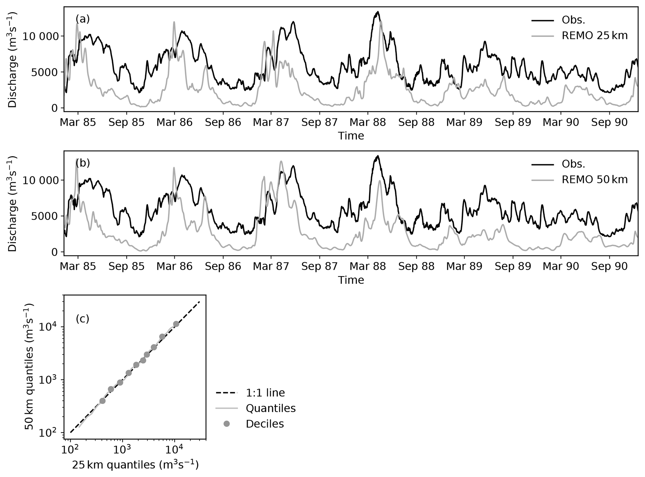
The same simulations as in Sect. 3.4 have been conducted with the REMO simulations created within the ENSEMBLES project. There are two main differences between the ENSEMBLES and the EURO-CORDEX simulations. First, the higher resolution is 25 km in ENSEMBLES, whereas it is 12 km in EURO-CORDEX. Second, ERA-40 is used as boundary condition in the ENSEMBLES project, whereas ERA-INTERIM is used in EURO-CORDEX. Interestingly, the bias of precipitation is less than 3 % for both resolutions used in the ENSEMBLES project, whereas it is 15 % for the 50 km run of EURO-CORDEX. However, the ENSEMBLES simulations show an underestimation of observed streamflow by up to 50 % (Fig. D1). This bias is reduced in the EURO-CORDEX simulations. A commonality between the EURO-CORDEX and ENSEMBLES simulations is that the absolute bias in streamflow is larger than the absolute bias in precipitation. This highlights that REMO overestimates evapotranspiration.

Figure D1 Same as Fig. 7, but using REMO simulations from the ENSEMBLES project.