Assessment of sub-shelf melting parameterisations using the ocean–ice-sheet coupled model NEMO(v3.6)–Elmer/Ice(v8.3)

Oceanic melting beneath ice shelves is the main driver of the current mass loss of the Antarctic ice sheet and is mostly parameterised in stand-alone ice-sheet modelling. Parameterisations are crude representations of reality, and their response to ocean warming has not been compared to 3-D ocean–ice-sheet coupled models. Here, we assess various melting parameterisations ranging from simple scalings with far-field thermal driving to emulators of box and plume models, using a new coupling framework combining the ocean model NEMO and the ice-sheet model Elmer/Ice. We define six idealised one-century scenarios for the far-field ocean ranging from cold to warm, and representative of potential futures for typical Antarctic ice shelves. The scenarios are used to constrain an idealised geometry of the Pine Island glacier representative of a relatively small cavity. Melt rates and sea-level contributions obtained with the parameterised stand-alone ice-sheet model are compared to the coupled model results. The plume parameterisations give good results for cold scenarios but fail and underestimate sea level contribution by tens of percent for warm(ing) scenarios, which may be improved by adapting its empirical scaling. The box parameterisation with five boxes compares fairly well to the coupled results for almost all scenarios, but further work is needed to grasp the correct number of boxes. For simple scalings, the comparison to the coupled framework shows that a quadratic as opposed to linear dependency on thermal forcing is required. In addition, the quadratic dependency is improved when melting depends on both local and non-local, i.e. averaged over the ice shelf, thermal forcing. The results of both the box and the two quadratic parameterisations fall within or close to the coupled model uncertainty. All parameterisations overestimate melting for thin ice shelves while underestimating melting in deep water near the grounding line. Further work is therefore needed to assess the validity of these melting parameteriations in more realistic set-ups.

1 Introduction

The majority of grounded ice in Antarctica is drained through its floating extensions advancing in the Southern Ocean. The increase in ice-mass loss since the 1990s has been mostly driven by ice-shelf thinning in the western part of the ice sheet (Paolo et al., 2015; Shepherd, 2018). In the Amundsen and Bellingshausen seas, ice-shelf thinning is due to incursions of Circumpolar Deep Water (CDW) beneath the ice-shelf base all the way to the line boundary between the grounded and floating part of the ice sheet, i.e. the grounding line. These incursions episodically increase the ocean–ice heat flux and drive sub-shelf melting and ice-shelf thinning (Jacobs et al., 2011; Dutrieux et al., 2014; Jenkins et al., 2018 for West Antarctica and Gwyther et al., 2018 for East Antarctica). The thinning of floating ice decreases the back force restraining the upstream ice, leading to ice-sheet acceleration (Mouginot et al., 2014), ice-surface lowering (Konrad et al., 2017), retreating grounding lines (Rignot et al., 2014; Konrad et al., 2018), and eventually increased sea level rise.

West Antarctic grounding lines often rest on retrograde bed up-sloping towards the ocean (Fretwell et al., 2013). This makes the glaciers vulnerable to the marine ice-sheet instability (MISI), which states that an ice sheet starting to retreat over a retrograde bed slope keeps retreating until the slope becomes prograde (Mercer, 1978; Thomas and Bentley, 1978; Weertman, 1974; Schoof, 2007; Durand et al., 2009). Confined ice shelves resist horizontal shearing and potentially stabilise an ice sheet undergoing MISI (Gudmundsson et al., 2012; Gudmundsson, 2013; Haseloff and Sergienko, 2018). Ice-sheet modelling results suggest that the Pine Island and Thwaites glaciers may have started an unstable retreat (Favier et al., 2014; Joughin et al., 2014), but the tipping point beyond which MISI occurs is not clearly identified (Pattyn et al., 2018).

Ocean warming is currently the main driver of the West Antarctic ice-sheet retreat, and can potentially trigger further MISI (Favier et al., 2014; Joughin et al., 2014). Using realistic ice-shelf basal melt rates in ice-sheet simulations is therefore crucial. The most comprehensive way to do so consists of using an ocean model that solves the 3-D Navier–Stokes equations in ice-shelf cavities and represents ocean–ice heat exchanges (Losch, 2008). The existence of strong feedbacks between the cavity geometry, melt rates, and the ocean circulation (De Rydt et al., 2014; Donat-Magnin et al., 2017) has motivated the development of coupled ocean–ice-sheet models presenting a moving ocean–ice boundary. To date, this kind of coupled model has been used in idealised configurations (e.g. De Rydt and Gudmundsson, 2016; Asay-Davis et al., 2016; Jordan et al., 2018; Goldberg et al., 2018) or with more realistic configurations representing a single ice shelf (Thoma et al., 2015; Seroussi et al., 2017). However, the required numerical developments and the relatively high computational cost of the ocean component strongly limit the use of ocean–ice coupled models for long-term simulations of the Antarctic ice sheet.

A much simpler approach to account for oceanic forcing in stand-alone ice-sheet models is to prescribe melting by plugging off-line ocean model outputs (e.g. Seroussi et al., 2014). The melt rates cannot evolve with cavity geometry changes. Mengel and Levermann (2014) improved the method by correcting the dependency of the freezing point to a changing ice draft, but it is still unable to account for the dependency on far-field temperature and salinity stratification, and for circulation changes driven by the evolution of the cavity geometry (Donat-Magnin et al., 2017). This approach also requires the choice of empirical ad hoc melt rates underneath newly floating ice wherever the grounding line is retreating during the prognostic simulations. To circumvent this issue, Cornford et al. (2015) and Nias et al. (2016) consider the ice-mass flux near and away from the grounding line to build a sound initial melting pattern that depends on the distance to the grounding line and adapts to its further migration. By construction, the melt rates are much larger at the grounding line and decrease exponentially away from it. Spatially and temporally varying melt rates (anomalies) taken from ocean models are added to these initial melt rates to predict future sea level contribution. This latter approach is also empirical and does not account for potential change in oceanic circulation (e.g. due to feedbacks with ice dynamical changes).

The melt rates can also be parameterised using two main approaches, being either an explicit function of depth or a function depending on far-field ocean temperature and salinity. In the first approach (followed by, for example, Favier et al., 2014; Joughin et al., 2014, with more examples given in Asay-Davis et al., 2017), they are computed by a piecewise linear function of depth, and an initial calibration is done to match current observations on average (e.g. using datasets from Rignot et al., 2013b; Depoorter et al., 2013). The oversimplicity of the depth dependence not only makes the initial pattern very different from the observed pattern, but also leads to a significant overestimation of the grounding-line retreat compared to ocean–ice-sheet coupled models (Seroussi et al., 2017; Jordan et al., 2018; De Rydt and Gudmundsson, 2016).

The second approach parameterises the melt rates as a function of ocean temperature and salinity profiles. The simplest parameterisations are mere functions of the difference between the temperature and the melting–freezing point at the ice–ocean boundary, the thermal forcing, using a linear (e.g. Beckmann and Goosse, 2003; Favier et al., 2016) or a quadratic dependency (e.g. DeConto and Pollard, 2016). More complexity is accounted for in the box model proposed by Reese et al. (2018a) and based on the 1-D ocean-box model from Olbers and Hellmer (2010), and also in the 2-D emulation of a 1-D plume model (Jenkins, 1991) proposed by Lazeroms et al. (2018).

Assessing these last parameterisations with regard to melt rates computed by a stand-alone ocean model would enable the patterns differences in a static cavity geometry to be investigated. However, the melt-rate pattern also has an effect on the ice-sheet response. The study of Gagliardini et al. (2010) highlights configurations where less melting leads to a grounding line relatively further upstream, or where the same average melting leads to two different ice-sheet responses and grounding-line positions. An ice-sheet model is therefore needed to carry out a meaningful comparison between parameterised and simulated melt rates.

In this paper, we assess several flavours of the aforementioned ocean temperature- and salinity-dependent parameterisations with regard to ocean–ice-sheet coupled simulations. We include the uncertainties arising from the ocean model by considering an ensemble of four ocean–ice coupled configurations. Following an initial calibration that allows further comparisons between parameterised and coupled simulations, we use six one-century far-field ocean temperature and salinity scenarios, which we apply to drive the melting parameterisations in stand-alone ice-sheet simulations and force the members of the ocean ensemble in ocean–ice-sheet coupled simulations. Overall, the MISOMIP (Asay-Davis et al., 2016) framework is used to perform 138 one-century simulations (19 sub-shelf melt parameterisations + 4 coupled members × 6 scenarios).

The paper is organised as follows. The second section describes the models: the ice-sheet model Elmer/Ice, the ocean model NEMO and the framework for coupling those two models. The section also describes the sub-shelf melt-rate parameterisations and the members of the ocean–ice ensemble. The third section describes the experiments, including the reference set-up of the ocean–ice-sheet system, the initial calibration of the parameterised and coupled simulations, and the set of far-field ocean temperature and salinity scenarios. Then in the fourth section, we detail the results with regard to sea-level contribution and sub-shelf melting evolution, and in the fifth section, we discuss the use of sub-shelf melt parameterisations in stand-alone ice-sheet modelling at a regional or a global scale.

2 Models

2.1 The ice-sheet model, Elmer/Ice

We perform the ice-sheet simulations with the finite-element ice-sheet model Elmer/Ice (Gagliardini et al., 2013). The ice rheology is non-linear and controlled by Glen's flow law (Appendix A), enabling the deviatoric stress tensor to be linked with the strain rate tensor from which ice velocities are retrieved. The version of the ice-sheet model used solves the SSA* solution, a variant of the L1L2 solution of Schoof and Hindmarsh (2010), solving the shallow shelf approximation of the Stokes equations and accounting for vertical shearing in the effective strain rate. The SSA* approximation was recently implemented in Elmer/Ice following the work of Cornford et al. (2015).

To calculate the basal friction, the grounding line position is calculated from hydrostatic equilibrium and can thus be located anywhere within an element. We use a sub-element parameterisation to affect basal friction to the part of the element that is grounded by increasing its number of integration points (equivalent to the SEP3 method in Seroussi et al., 2014). The basal friction is computed by a Schoof-like friction law based on the theoretical work of Schoof (2005) applied to a linear ice rheology, and which was extended to a non-linear rheology by Gagliardini et al. (2007). The Schoof friction law (Appendix A) depends on the effective pressure, the difference between the ice overburden pressure and the basal water pressure, here approximated by the ocean pressure. This friction law therefore exhibits two asymptotic behaviours, behaving as a non-linear power law away from the grounding line and as a Coulomb friction law near the grounding line, and thus ensuring a smooth transition of stress state near and at the grounding line. The Schoof friction law was recently compared to various other types of friction laws commonly used in ice-sheet modelling, for an idealised framework (Brondex et al., 2017) and a real drainage basin (Brondex et al., 2018).

Melting is applied to floating nodes but not to grounded nodes, meaning that the first floating element (partially or not) may be affected by melting. The mesh grid is unstructured and made of triangles, the size of which is about 500 m in the vicinity of the grounding line and up to 4 km away. The Elmer/Ice configuration is identical for parameterised and coupled simulations.

2.2 Ocean melting from a 3-D ocean–ice-sheet coupled model

The melt rates beneath the ice shelf are either parameterised or computed through the coupling of NEMO and Elmer/Ice. Here we describe the ocean model and the ocean–ice-sheet coupling framework.

2.2.1 The ocean model, NEMO

We make use of the 3-D primitive-equation ocean model NEMO-3.6 (Nucleus for European Modelling of the Ocean; Madec and NEMO-team, 2016). NEMO solves the prognostic equations for the ocean temperature, salinity, and velocities and includes ice-shelf cavities (Mathiot et al., 2017). The sub-shelf melting is parameterised through the so-called “three equations” representing (1) the heat balance at the ice–ocean interface accounting for phase change, turbulent exchange in water, and diffusion in the ice; (2) the salt balance accounting for freezing, melting, and turbulent exchange; and (3) the pressure and salinity dependence of the potential temperature at which seawater freezes (Hellmer and Olbers, 1989; Holland and Jenkins, 1999; Losch, 2008; Jenkins et al., 2010). In this parameterisation, we assume a constant top-boundary-layer (TBL) thickness along the ice-shelf draft (Mathiot et al., 2017), and we use a velocity-dependent formulation in which the heat exchange velocity is defined as follows:

$$\begin{array}{}\text{(1)}& {\mathit{\gamma }}_T={\mathrm{\Gamma }}_T\sqrt{C_{\mathrm{d}}(u_{\text{TBL}}^{\mathrm{2}}+u_{\mathrm{tide}}^{\mathrm{2}})},\end{array}$$

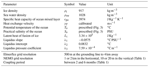
where u_TBL the TBL-averaged velocity resolved by NEMO, Γ_T is the non-dimensional heat exchange coefficient, C_d the non-dimensional drag coefficient and u_tide is a uniform background velocity representing the main effect of tides on ice-shelf melting (Jourdain et al., 2018). The values of Γ_T, C_d, and u_tide are given in Table 1.

The ocean configuration used in this study is very similar to the ISOMIP+ configuration described by Asay-Davis et al. (2016): we use a linearised equation of state and the only lateral boundary condition is a temperature and salinity restoration along the vertical boundary representing offshore conditions; neither sea ice nor atmospheric forcing nor tides are represented. The only differences with the general MISOMIP protocol is that we use different temperature and salinity restoration and initial conditions (Sect. 3.3). We use a variety of resolutions and parameters for NEMO to build an ensemble of NEMO-Elmer/Ice coupled simulations as described in Sect. 2.2.3.

2.2.2 The ocean–ice-sheet coupled model framework

We couple NEMO and Elmer/Ice, meaning that Elmer/Ice sees sub-shelf melt rates calculated by NEMO, while NEMO sees the ice-shelf geometry resulting from the ice dynamics resolved by Elmer/Ice. A given coupling period (typically of few months) is first covered by the ocean model with the cavity geometry from the end of the previous coupling period; then, the period is covered by the ice-sheet model forced by the oceanic melt rates averaged over this coupling period in order to conserve mass as much as possible (Fig. 1).

Figure 1 NEMO-Elmer/Ice coupling framework. T and S stand for temperature and salinity.

As the respective grids of the two models differ, some interpolation is required for each exchange. Following each NEMO run, Elmer/Ice restarts from its previous time step (ice geometry and velocities). The melt rates provided by NEMO are bi-linearly interpolated onto Elmer/Ice's unstructured grid. A multiplicative correction factor computed over the entire ice shelf ensures that the same mass flux is seen by the two models (this factor is very close to one in our case). In case Elmer/Ice has a floating element but the water column is too thin to be captured by NEMO (a minimum thickness of 20 m allows NEMO to have a minimum of two vertical cells under the partial cell conditions, Mathiot et al., 2017), the melt rate seen by Elmer/Ice is set to zero.

Every coupling period, NEMO restarts with temperature, salinity, and velocities from its previous time step using the updated geometry from Elmer/Ice. If new ocean cells appear (previously masked ice cells), temperature and salinity are an average of the four closest wet cells (horizontally if possible, vertically extrapolated otherwise), and ocean velocities are set to zero. To avoid the generation of spurious barotropic waves as a result of sudden changes in water column thickness, we impose a conservation of barotropic velocities across the step change in the ice-shelf geometry. We also conserve the sea surface height (SSH) value for all the water columns, and if a new water column is created, SSH is an average of the four closest wet cells.

We use the same initial state for Elmer/Ice as in MISOMIP (Asay-Davis et al., 2016), i.e. a steady state obtained with zero melt, and NEMO is spun up for 5 years with this initial ice-shelf geometry before being coupled to Elmer/Ice. The respective time steps of Elmer/Ice and NEMO are 1 month and 200 s, and the coupling period ranges between 2 and 6 months, depending on the configuration. We performed a sensitivity study following the MISOMIP protocol (Asay-Davis et al., 2016), which indicates very little sensitivity to coupling periods between 1 month and 1 year, with less than 3 % difference in sea-level contribution after 100 years (Appendix B).

2.2.3 The ensemble of ocean configurations within the coupled framework

While the NEMO ocean model is much more representative of the ocean physics than any sub-shelf melting parameterisation, there are still processes like turbulence and convection that need to be parameterised. The model is also sensitive to both the horizontal and vertical resolutions. To account for the consequent ocean model uncertainty, we consider four NEMO configurations with the varying parameters listed in Table 1. For each coupled configuration, the Γ_T parameter is adjusted following the exact ISOMIP+ calibration protocol after 4 years of ocean spin-up with a steady ice-shelf draft (more details of the protocol relevant to our study are given in Sect. 3.2, and the protocol is fully described in Asay-Davis et al., 2016; Sect. 3.2.1).

Table 1 Ocean parameters used for the four NEMO-Elmer/Ice coupled simulations. Δx is the horizontal resolution, T_CPL is the ocean–ice-sheet coupling period and Δz is the nominal vertical resolution. The actual resolution near the sea floor or ice shelf draft can be smaller due to the use of partial steps, but the TBL thickness is always equal to Δz (i.e. TBL quantities are averaged over several levels in the case of partial steps). Γ_T and u_tide are defined in Eq. (1), and the salt exchange coefficient Γ_S is taken as Γ_T∕35. Also defined in Eq. (1) is the drag coefficient $C_{\mathrm{d}}=\mathrm{2.5}\times {\mathrm{10}}^{-\mathrm{3}}$ . The stable vertical diffusivity and viscosity coefficients (K_stab and ν_stab respectively) are either constant, at the same values as in Asay-Davis et al. (2016), or calculated through the TKE scheme with the same parameter values as in Treguier et al. (2014). Convection is parameterised through enhanced diffusivity and viscosity (K_unstab and ν_unstab respectively) in case of static instability (0.1 m² s⁻¹ as Asay-Davis et al., 2016 and 10 m² s⁻¹ as Treguier et al., 2014). The remaining parameters are exactly the same as in the common ISOMIP+ configuration described in Asay-Davis et al. (2016).

2.3 Ocean melting from ocean-dependent sub-shelf parameterisations

All the parameterisations are linked to ambient temperature and salinity vertical profiles in the far-field ocean. The stand-alone ice-sheet simulations start from the same initial state as for the ocean–ice-sheet coupled simulations. The parameterisations respond instantaneously to changes in ambient temperatures and salinities; i.e. they do not account for ocean circulation timescales (e.g. water residence time in ice-shelf cavities, Holland, 2017). None of the parameterisations account for the Coriolis effect or for bathymetric features (e.g. sills, channels). To avoid areas of very thin ice that would affect the stability of the ice-sheet model, melting is not permitted wherever the ice base is shallower than 10 m depth.

2.3.1 Simple functions of thermal forcing

The following three parameterisations are based on an expression for the ice–ocean heat transfer that is analogous to the one used in more complex ocean circulation models (Grosfeld et al., 1997). However, they make the simplifying assumption that the thermal forcing across the ice–ocean boundary layer can be determined directly from far-field ocean conditions. Thus, cooling of the water as it is advected from the far field into the cavity and then mixed into the ice–ocean boundary layer is accounted for simply through the choice of an effective heat transfer coefficient.

The linear, local dependency on thermal forcing assumes a balance between vertical diffusive heat flux across the ocean cavity top boundary layer and latent heat due to melting and freezing. Its formulation is based on Beckmann and Goosse (2003) and written as follows:

$$\begin{array}{}\text{(2)}& M_{\mathrm{lin}}={\mathit{\gamma }}_T{\displaystyle \frac{{\mathit{\rho }}_{\mathrm{sw}}{c}_{\mathrm{po}}}{{\mathit{\rho }}_{\mathrm{i}}{L}_{\mathrm{i}}}}(T_{\mathrm{o}}-T_{\mathrm{f}}),\end{array}$$

with γ_T the heat exchange velocity (aimed at being calibrated; see Sect. 3.2), ρ_sw and ρ_i the respective densities of ocean water and ice, c_po the specific heat capacity of the ocean mixed layer, and L_i the latent heat of fusion of ice (Table 2). The melting–freezing point T_f at the interface between the ocean and the ice-shelf basal surface is defined as follows:

$$\begin{array}{}\text{(3)}& T_{\mathrm{f}}={\mathit{\lambda }}_{\mathrm{1}}{S}_{\mathrm{o}}+{\mathit{\lambda }}_{\mathrm{2}}+{\mathit{\lambda }}_{\mathrm{3}}{z}_{\mathrm{b}}.\end{array}$$

The practical salinity S_o and the potential temperature T_o are taken from the far-field ocean as detailed below in this section; z_b is the ice base elevation, which is negative below sea level; and the coefficients λ₁, λ₂, and λ₃ are respectively the liquidus slope, intercept, and pressure coefficient.

The linear formulation with a constant exchange velocity assumes a circulation in the ice-shelf cavity that is independent from the ocean temperature. This assumption is neither supported by modelling (Holland et al., 2008; Donat-Magnin et al., 2017) nor by observational studies (Jenkins et al., 2018) that suggest a more vigorous circulation in response to a warmer ocean, subsequently increasing melt rates.

The quadratic, local dependency on thermal forcing accounts for this positive feedback between the sub-shelf melting and the circulation in the cavity (Holland et al., 2008), using a heat exchange velocity linearly depending on local thermal forcing. The formulation is written as follows:

$$\begin{array}{}\text{(4)}& M_{\mathrm{quad}}={\mathit{\gamma }}_T{\left({\displaystyle \frac{{\mathit{\rho }}_{\mathrm{sw}}{c}_{\mathrm{po}}}{{\mathit{\rho }}_{\mathrm{i}}{L}_{\mathrm{i}}}}\right)}^{\mathrm{2}}(T_{\mathrm{o}}-T_{\mathrm{f}}{)}^{\mathrm{2}}.\end{array}$$

These last two parameterisations were used in numerous studies (e.g. review in Asay-Davis et al., 2017). As the ocean properties used to calculate melting for every draft point are taken at the very same point, they are tagged as local.

The quadratic, local and non-local dependency on thermal forcing is a new parameterisation assuming that the local circulation (at a draft point) is not only affected by local thermal forcing, but also by its average over the ice basal surface, which is written as follows:

$$\begin{array}{}\text{(5)}& M_{+}={\mathit{\gamma }}_T{\left({\displaystyle \frac{{\mathit{\rho }}_{\mathrm{sw}}{c}_{\mathrm{po}}}{{\mathit{\rho }}_{\mathrm{i}}{L}_{\mathrm{i}}}}\right)}^{\mathrm{2}}(T_{\mathrm{o}}-T_{\mathrm{f}})〈T_{\mathrm{o}}-T_{\mathrm{f}}〉.\end{array}$$

This formulation is inspired by Jourdain et al. (2017), who showed an overturning circulation proportional to total melt rates. It is equivalent to assuming that melting is first generated by local thermal forcing, and that this first-guess melting generates a circulation at the scale of the ice-shelf cavity that feeds back on melt rates. In other words, this formulation reflects the three equations with a uniform exchange velocity that is proportional to the cavity-average thermal forcing.

In Eqs. (2), (4), and (5), the values of T_o and S_o are either depth-dependent or taken from a constant depth in the far field (Sect. 3.3 details the different far-field ocean temperature and salinity vertical profiles). The former situation (for which T_o=T_o(z) and S_o=S_o(z)) assumes a horizontal circulation between the far-field ocean and the ice draft that would transport constant ocean properties. This can be viewed as an asymptotic case where the circulation in the cavity is driven by tides rather than melt-induced buoyancy forces, which is equivalent to the aforementioned three equations with a constant and uniform velocity along the ice base. Alternatively, in the latter situation, T_o and S_o are taken at either 500 m or 700 m depths, i.e. near the sea floor. This assumes that ocean water is advected into the cavity along the sea floor up to the grounding line, then upward along the ice base with constant ocean temperature and salinity.

The value of T_f is therefore calculated with either S_o(z) in the first option, or S_o(500) or S_o(700) in the second option (in a consistent way with T_o), but with the local ice base depth. For each far-field ocean temperature and salinity profile, we thus run three Elmer/Ice simulations for each simple function of the thermal forcing.

Table 2 Physical parameters, model grid resolutions, and coupling period.

(Reese et al., 2018a)(Lazeroms et al., 2018)

Table 3 Parameterisations used to compute melting in stand-alone ice-sheet simulations. The last column lists the calibrated γ_T obtained from the WARM profile, except for the plume parameterisation where a multiplicative coefficient α is used instead.

2.3.2 More complex functions of thermal forcing

The following two parameterisations attempt to improve on the above by including a representation of some of the processes that determine the temperature within the ice–ocean boundary layer. Cooling of the water as it is advected into the cavity is still neglected, so that the waters incorporated into the boundary layer have far-field properties. However, cooling of the boundary layer by melting at depth, the rise of the waters along the ice shelf base, and the change in the freezing point with depth are all considered with different levels of detail. Critically, including such processes enables these parameterisations to simulate regions of basal freezing, something that the simple functions of far-field temperature cannot reproduce.

The box parameterisation was developed by Reese et al. (2018a) based on the analytical steady-state solution of the box model of Olbers and Hellmer (2010). The latter, initially developed for a 2-D cavity, represents the buoyancy-driven advection of ambient ocean water into the ice-shelf cavity at depth up to the grounding line, then upward along the ice draft in consecutive boxes. The melt rates are given by the following:

$$\begin{array}{}\text{(6)}& \mathrm{BM}={\mathit{\gamma }}_T{\displaystyle \frac{{\mathit{\rho }}_{\mathrm{sw}}{c}_{\mathrm{po}}}{{\mathit{\rho }}_{\mathrm{i}}{L}_{\mathrm{i}}}}(T_k-T_{\mathrm{f},k}),\end{array}$$

where the k subscript indicates properties evaluated in each box. Those properties account for the transformation of ocean temperature and salinity in consecutive boxes through heat and salt turbulent exchange across the ocean boundary layer underneath ice shelves. Hence, the box model is entirely driven by ocean temperature and salinity near the sea floor. Unlike plume models, the box model does not entrain deep water all along the upward transport, it advects deep water from the open ocean to the grounding zone then transports it upward. Therefore, this parameterisation produces maximum melt rates near the grounding line.

A key assumption is that the overturning circulation (i.e. volume transport through the boxes) is taken proportionally to the density difference between the ambient ocean (open ocean seaward of the ice shelf) and the deepest box including an ocean–ice interface. Similarly to the simple parameterisations, the box model assumes constant heat and salt exchange velocities.

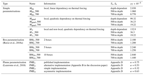
In their implementation, Reese et al. (2018a) calibrated both the heat exchange and overturning coefficients to obtain realistic melt rates for both the Pine Island and Ronne-Filchner ice shelves. Here, we keep the overturning coefficient used by Reese et al. (2018a), and we calibrate the effective heat exchange velocity in the same way as the other parameterisations (Sect. 3.2).

In our implementation of the box model, the calving front position that is used to build the boxes' positions is considered to be at either x=640 km or defined by the 10 m depth contour, the limit below which no melting is permitted for the ice-sheet model. In the Reese et al. (2018a), the dependence of sub-shelf melting on the local pressure due to the vertical ice column induces a lack of energy conservation. We thus decided not to implement this dependence, resulting in a uniform melting within each box.

For each temperature and salinity scenario, we run six Elmer/Ice simulations using the box parameterisation, with either 2, 5, or 10 boxes, and with ocean temperature and salinity taken at constant depths of either 500 or 700 m.

The plume parameterisation developed by Lazeroms et al. (2018) emulates the 2-D behaviour of the 1-D plume model proposed by Jenkins (1991). This model describes the evolution of a buoyant plume originating from the grounding line with zero thickness and velocity, and temperature and salinity taken from the ambient ocean. Away from the grounding line, the thickness, velocity, temperature, and salinity of the plume evolve through advection, turbulent exchange across the ocean boundary layer underneath the ice shelf, and entrainment of deep water. Among the melt formulations presented in this paper, the plume parameterisation is the only one to include velocity-dependent heat and salt exchange velocity. No background or tidal velocity is prescribed, so turbulent exchanges and melt rates are zero right at the grounding line.

The plume model can be scaled with external parameters and applied to 1-D ice drafts of any slope, ambient temperature, and salinity (Jenkins, 2014). The melt rates are given by the following:

$$\begin{array}{}\text{(7)}& \text{PME}=\mathit{\alpha }{M}_{\mathrm{o}}g\left(\mathit{\theta }\right)(T_{\mathrm{o}}-T_{\mathrm{f},\mathrm{gl}}{)}^{\mathrm{2}}\widehat{M}(\widehat{X}),\end{array}$$

where PME means plume model emulator; M_o is an overall scaling parameter; g(θ) is a function of the ice-shelf basal slope θ, but also of physical constants (heat exchange coefficient, drag coefficient, and entrainment); the f, gl subscript indicates the freezing temperature at the depth of the grounding line; and the final term gives the scaled melt rate, $\widehat{M}$, as a universal function of scaled distance, $\widehat{X}$, that was derived from empirical fitting of results generated by the full plume model on idealised geometries (Jenkins, 2014). α is a multiplicative coefficient that will be used for calibrating purposes in our study (see further details in this section). The far-field temperature used here is taken at the depth of the grounding line, as in the box model, and enters the parameterisation explicitly because the subsequent evolution of the ice–ocean boundary layer temperature through entrainment of the far-field ocean, melting, and freezing is captured through the slope-dependent scaling and the universal function. The non-linear dependence on temperature arises because the melt rates depend on the product of plume temperature and plume speed. The latter is a function of the plume buoyancy, which is itself linearly dependent on plume temperature. The physical basis for the scaling is discussed further in Appendix C, but we note here that when the ice-shelf basal slope and far-field conditions are non-uniform, there is no longer a unique choice for those variables in the parameterisation, and choices other than the ones used in this study are equally valid.

Another major issue with the plume parameterisation is the transition from a 1-D to a 2-D ice draft. It is indeed difficult to identify the pathway from a given location of the ice draft to the grounding line point where the plume has emerged, which is enhanced by the fact that several plumes may end up at a given location. To define effective pathways, we apply 4 empirical methods that are all based on different calculations of effective values for the grounding line depth and the basal slope. The first method was originally published in Lazeroms et al. (2018) and applied to a structured grid. The second method was proposed in the corresponding discussion paper but finally discarded to simplify the publication. The last two methods propose simpler ways to calculate the effective grounding-line depth and basal slope. All the methods and their adaptation to unstructured grids are described in Appendix D.

The plume parameterisation from Lazeroms et al. (2018) includes a heat exchange coefficient that is a function of the plume velocity along the ice-shelf base, which is similar to the ocean model but not to the other parameterisations. The complexity of this parameterisation motivated us to calibrate it by adding a multiplicative coefficient α (Table 3) to the melt expression (Eq. 7) rather than calibrating physical parameters.

For each temperature and salinity scenario, we run four Elmer/Ice simulations with the plume parameterisation, using the four aforementioned methods to calculate the effective plume pathway (Appendix D) and with ambient temperature and salinity taken at the effective grounding line depth (as defined in  Lazeroms et al., 2018).

3 Experiments

3.1 Initial geometry and set-up

We simulate the evolution of an ideal ice-sheet inspired by the Pine Island glacier in West Antarctica. The domain is the same as the MISOMIP domain for the coupled simulations and as the MISMIP+ domain for the stand-alone ice-sheet simulations (Asay-Davis et al., 2016). The ice sheet is marine based and its grounding line rests on a retrograde bed sloping upward towards the ocean. The entire domain, including the ice sheet and the ocean, is 800 km long and 80 km wide (Fig. 2). The ice-sheet calving front is located at x=640 km, while the remaining domain, up to x=800 km, and also the cavity beneath the ice shelf are filled with ocean water. The ice sheet is in equilibrium state with an accumulation rate of 0.3 m a⁻¹ and no sub-shelf melting, as required by MISMIP+, using the ice-sheet configuration detailed in Sect. 2.1. The initial grounding line central position is x=450 km.

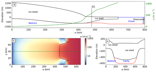
Figure 2 Initial ice-sheet in equilibrium calculated by Elmer/Ice with an accumulation rate of 0.3 m a⁻¹ and no sub-shelf melting as required by the MISMIP+ protocol (Asay-Davis et al., 2016). (a) Side-view geometry in the central flow line, also indicating the position of the ocean restoration used by the ocean model, and the velocity magnitude along the central flow line shown in panel (b). (b) Velocity magnitude seen from above. The black solid line indicates the grounding line. (c) Cross section of the ice sheet at x=480 km.

3.2 Initial state and calibration

The initial calibration purpose is to assess whether the parameterisations represent the response of melt rates to changing ocean temperature and salinity. We thus make sure that all the parameterised and coupled configurations produce the same melting average for the WARM profile of MISOMIP (Fig. 3; Asay-Davis et al., 2016).

This average is obtained through a spin-up of the ocean model applied to the initial ice-shelf draft (Fig. 2 and Sect. 3.1) and performed before further coupled simulation (Fig. 1). We follow the ISOMIP+ protocol (Asay-Davis et al., 2016) to achieve the required sub-shelf melt rate average of 30±2 m a⁻¹ below 300 m depth after 4 years of ocean spin-up. The value of Γ_T, which is not known with accuracy and is usually calibrated in ocean models (Asay-Davis et al., 2016; Jourdain et al., 2017), is therefore adjusted to achieve these melt rates (Table 1). The remaining steps of our calibration, described here below, differ from the ISOMIP+ protocol and are specific to our study. We compute the melting average of all four configurations over the ice draft (excluding parts shallower than 10 m for which no melt is applied), which gives 〈m_t8.5± m a⁻¹. These four spin-ups will thus be used as initial states for subsequent coupled simulations.

Then, 〈m_t〉 is used as a target for stand-alone ice-sheet simulations forced by the WARM profile from the ISOMIP+/MISOMIP protocol. For the parameterisations in which γ_T is constant (Eq. 1), we achieve the target by adjusting γ_T. For the plume parameterisation, which accounts for a top boundary layer velocity, we adjust the value of the multiplicative coefficient α (calibrated values shown in Table 3) to achieve the same target (see Sect. 2.3).

The reason why we did not calibrate the parameterisations to reproduce the average melt rates below 300 m as done in MISOMIP is because all of them produce substantial melt rates underneath the shallowest parts of the ice shelf, as opposed to the ocean models. To emphasise this point, we also performed the simulations with the calibration done as in MISOMIP below 300 m depth, the results of which are given in Appendix F.

The WARM profile was put forward in MISOMIP because it enables a short spin-up of the ocean model, which is useful for calibration purposes as here. After this calibration phase, we keep the calibration reported in Table 2 for all the one-century scenarios described in Sect. 3.3.

3.3 The set of ocean temperature and salinity scenarios

We consider the following six scenarios over a century (Fig. 3), the first two being kept constant, and the other four linearly evolving in time:

• Warm₀ resembles the present-day typical Amundsen Sea conditions (Dutrieux et al., 2014). There is no temporal change of temperature and salinity profiles.

• Warm₁ starts from the Warm₀ profile and then the temperature uniformly increases by 1 ^∘C per century. The salinity profile is constant in time.

• Warm₂ is similar to Warm₁ but the warming rate increases with depth, from zero in the surface layer to 1 ^∘C per century below the deep thermocline. The salinity profile is constant in time.

• Warm₃ starts from the Warm₀ profile and undergoes a 200 m uplift of both the thermocline and the halocline.

• Cold₀ resembles a cold cavity such as beneath the Ronne-Filchner ice shelves. There is no temporal change of temperature and salinity profiles.

• Cold₁ starts from the Cold₀ profile and then warms to reach a warm cavity state within a century. The salinity is also increased.

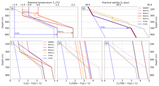
Figure 3 Far-field ocean temperature (a) and salinity (b) profiles scenarios in front of the cavity. The WARM profile is used for calibrating the initial state of parameterised and coupled simulations. The Warm₀ and Cold₀ scenarios are constant in time, while the others evolve linearly in time following the arrows. The Warm₁, Warm₂, and Warm₃ scenarios start with the Warm₀ profile and end up after a century in their respective profiles, while the Cold₁ scenario starts from the Cold₀ profile. In (b), profiles Warm₀, Warm₁, and Warm₂ are equal. Thermal forcing is calculated from the far-field temperature and salinity and applied to the ice-shelf draft, (c) assuming horizontal circulation between the far-field ocean and the cavity or assuming that the circulation is driven by oceanic properties at (d) 500 m and (e) 700 m depths. Profiles from the (c) panel are superimposed to panels (d) and (e) as a watermark for comparison purposes. The Warm₁ and Warm₂ profiles are equal in panel (e).

These profiles are slightly more realistic than in MISOMIP. They all include a thermocline, because its importance in ice-shelf melting has been pointed out by previous studies (e.g. De Rydt et al., 2014). The Warm₀ profile corresponds to a linear representation of the average hydrographic profiles measured in front of Pine Island glacier (Dutrieux et al., 2014). By contrast, the Cold₀ profile represents typical cold-cavity conditions in which deep ocean convection associated with sea ice formation prevents the stratification (e.g. for the Ronne-Filchner and Ross ice shelves). The Warm₁ scenario leads to 1 ^∘C warming at all depths after 100 years, which corresponds to the upper 80th to 90th percentile of ocean warming projected in the Amundsen Sea by 33 CMIP5 models (Appendix E). The Warm₂ scenario is more conceptual and assumes that the sea ice cover will persist over 100 years, i.e. that the ocean surface remains close to the freezing point while the subsurface gets warmer. The Warm₃ scenario is inspired by the study of Spence et al. (2014) suggesting that poleward shifting winds over the 21st century will uplift the coastal thermocline due to decreased Ekman downwelling. Last, the Cold₁ scenario is an idealised representation of the ocean tipping point described by Hellmer et al. (2012, 2017), in which the Ronne-Filchner cavities switch from a cold to a warm state.

The salinity profile is unchanged throughout Warm₀, Warm₁, and Warm₂ and is sufficiently stratified to keep a stable density profile. In the Warm₃ scenario, the halocline is lifted together with the thermocline to mimic an Ekman-driven uplift of the pycnocline, and in Cold₁, the stratification in salinity is increased linearly in time to keep a stable stratification when the cavity switches from cold to warm states. Note that none of the temperature profiles account for a salinity compensation (as opposed to the MISOMIP protocol), so the density profile is different in each scenario.

Figure 3c–e show the thermal forcings applied to stand-alone ice-sheet simulations for the different hypotheses for temperature and salinity inputs (Sect. 2.3), while Table 3 summarises the ensemble of sub-shelf melting parameterisations.

4 Results

4.1 Melting patterns resulting from the initial calibration

The calibrated parameters are given in Table 3 and the melting patterns are shown in Fig. 4 (not all the patterns are shown). The patterns obtained from the coupled and parameterised simulations are quite different, even though all of them result in similar cavity melt rates. The coupled simulations give the most melting below approximately 300 m depth and almost no melting near the ocean surface, which also highlights why the calibration was performed below 300 m depth in ISOMIP+ (Asay-Davis et al., 2016). The parameterised simulations give significant melt rates at all depths.

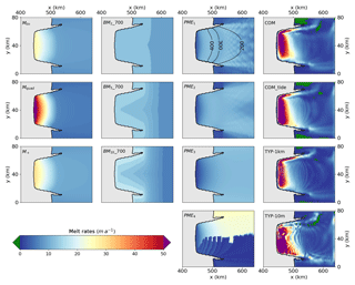
Figure 4 Diagnostic sub-shelf melt rates obtained through the calibration process by forcing the coupled and the parameterised models with the WARM profile from Asay-Davis et al. (2016). All the ocean members are represented (last column) but not all the parameterisations (first three columns). The average melting for every parameterisation equals 8.5 m a⁻¹, while being in the range 8.5± 1 m a⁻¹ for the ocean members. In the PME₁ panel the 200, 300, and 400 m draft contours are shown. The grounded ice is coloured in grey.

Near the grounding line, melt rates higher than 50 m a⁻¹ are predicted by all coupled simulations, while this value is only and hardly reached by the M_quad parameterisation and never reached in the other cases. Away from the grounding line, where the ice shelf is also thinner, melt rates are close to zero for the coupled simulations while they mostly remain above 10 m a⁻¹ when parameterised. Such differences in melt rate patterns are expected to induce diverging responses from the ice sheet (Gagliardini et al., 2010; Reese et al., 2018b).

While the patterns in the coupled simulations are quite similar to each other, the parameterised patterns differ to various extents. The parameterisations that have a simple dependence on thermal forcing (i.e. M_lin, M_quad, and M₊) compute the highest melt rates at depth, which also falls close to the grounding line in the central flow line. They also result in a rather uniform pattern when the basal surface is closer to the sea surface, which occurs away from the grounding line in the central flow line but also close to the grounding line on the sides of the ice shelf, where two bits (or horns) of grounded ice penetrate seaward. The range of melt rates is wider for the M_quad parameterisation, thinner ice being less melted and thicker ice being more melted, compared to M_lin and M₊. The M_lin and M₊ patterns are similar by construction because the melting average is driven by the (T_o−T_f) term, which appears only once in the two respective formulations. However, the respective calibrations are different (Table 3) because of the term 〈T_o−T_f〉 appearing in M₊ only, and the sensitivity to ocean warming will therefore be different.

The implementations of the 2-D plume emulator produce quite different patterns between PME₁, PME₂, and PME₃ on the one hand and PME₄ on the other hand, mostly because the latter is highly asymmetric. In the first three implementations, the different approaches adopted to calculate the effective depth and angle (Lazeroms et al., 2018) all result in very similar patterns. They all induce zero to small melt rates near the central grounding line because the valid directions are associated with low basal slopes. However, along the sides of the main trunk, on the inner side of the horns, the melt rates get higher at the grounding line because the plumes mostly emerge from the central, much deeper part of the grounding line, and not from the sides where the basal surface is higher than the draft point (PME₁ in Fig. 4). Farther away, PME₁ and PME₂ produce a slight decrease in melting near the calving front, which reflects the empirical scaling with the distance to the grounding line made in Lazeroms et al. (2018) and may not be adapted to our relatively small ice shelf. In the PME₃ parameterisation, the plume arises only from the deepest grounding line, whatever the position in the ice draft. On the external sides of the domain, it induces strong melting compared to PME₁ and PME₂ for which the plumes can also come from less deep parts of the cavity and mitigate the melt rates.

Similarly to the M_lin, M_quad, and M₊ parameterisations, the box parameterisation produces its highest melt rates near the grounding line. Away from the grounding line, the melt rates get lower to end up with the lowest values close to the calving front. The larger the number of boxes, the larger the melt rates near the grounding line, and the smaller the melt rates near the calving front.

4.2 Ice-mass loss and sub-shelf melt rates

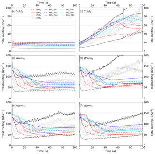
The initial ice sheet is built within the framework of MISMIP+ (Asay-Davis et al., 2016), requiring no sub-shelf melting, and is thus in equilibrium under such conditions. The simulations thus all start with an initial dynamical adjustment of the ice-sheet geometry to new ocean conditions (Fig. 4), which generates a melting pulse despite the 5 years of ocean spin-up. The adjustment is larger for relatively warmer scenarios (Figs. 5, 6). The pulse is therefore much lower and hardly visible for the Cold₁ scenario and only shows for the coupled simulations and not for the parameterised simulation for the Cold₀ scenario. For the Warm_i scenarios, the peak of the pulse yields similar melting of up to 130 Gt a⁻¹ for parameterised and coupled simulations. However, it lasts longer for the former, about 20 a, than for the latter, about 5 a. The pulse in coupled simulations quickly adds a lot of fresh water in the cavity, which further decreases melting. Such feedback is either not or poorly accounted for in the parameterisations, thus increasing the duration of the pulse compared to the coupled simulations.

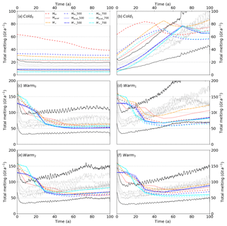
Figure 5 Total melt rates for simple parameterisations (Sect. 2.3.1). The coupled simulations are shown in solid light grey. The coloured lines correspond to parameterised simulations. The black solid lines correspond to a 50 % underestimation or overestimation compared to the average of coupled runs members.

Figure 6 Similar to Fig. 5 but for more complex parameterisations (Sect. 2.3.2).

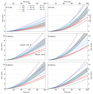
In the Cold₀ scenario, almost all parameterised and coupled simulations produce constant melt rates. Only the M_lin parameterisations produce very high melt rates at the start and decrease monotonically afterwards. In the other constant scenario, which is Warm₀, the pulse is followed by a decrease in melting, which becomes constant after tens of years for most parameterisations, as opposed to the coupled simulations where the melt rates slightly increase up to the end. In the other scenarios, which are all warming in some way, the pulse is always followed by a melting minimum, after which almost all the parameterised melt rates slightly increase up to the end (there are few exceptions where they are more constant, e.g. M_lin_700 forced by Warm₃). Finally, the Warm_i scenarios end up with between 40 and 175 Gt a⁻¹ of melting and the Cold₁ scenario with between 50 and 100 Gt a⁻¹ of melting. This means that the ice-sheet is contributing 4 to 12 mm to the sea level equivalent mass for the Warm_i scenarios, 2 to 4 mm for the Cold₁ scenario and 0.5 to 3 mm for the Cold₀ scenario (Figs. 7, 8).

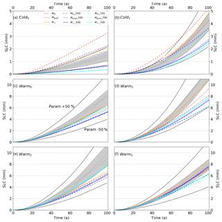
Figure 7 Sea level contribution (SLC) for simple parameterisations (Sect. 2.3.1). The coupled simulations are shown in solid light grey and their envelope in grey shading. The coloured lines correspond to parameterised simulations. The black solid lines correspond to a 50 % underestimation or overestimation compared to the average of coupled run members.

Figure 8 Similar to Fig. 7 but for more complex parameterisations (Sect. 2.3.2).

For the Warm_i scenarios, the parameterisations in general tend to overestimate the melting close to the sea surface and underestimate it at depth. This results in initially melting a large part of thinner ice, which makes overall melting higher compared to coupled simulations. Along with the disappearance of thinner ice, the overall melting becomes progressively lower than for coupled simulations. In the end, this results in lower sea level contribution (SLC) from the parameterised simulations, apart from few exceptions. In the Cold_i scenarios, melting is never high enough to completely remove thin ice and the SLC from parameterised simulations is more in agreement with the coupled simulation on average.

The uncertainties linked to the ocean model are emphasised by the spread of SLC calculated from the coupled model. The spread is about ± 10 % around the average for all the scenarios except for the Cold₀ and Warm₂ scenarios, where it is about ± 20 %, respectively. A larger spread of about ± 30 % for the Warm_i scenarios, and about ± 50 % and ± 100 % for the Cold₁ and Cold₀ scenarios, respectively, is obtained from the parameterisations, which reflects the wide variety of approaches and indicates that it makes sense to inter-compare parameterisations with respect to the coupled model.

Whatever the type of hypothesis for the depth at which the far-field ocean temperature and salinity profiles are taken (Sect. 2.3), the M_lin parameterisations tend to largely overestimate the melt rates for the Cold_i scenarios and underestimate them for the Warm_i scenarios, leading to respective overestimation and underestimation of SLC. This reflects a poor representation of melting by these parameterisations when the change in ocean forcing is too large.

The M_quad parameterisations give melting in fair agreement with coupled results for the Cold_i scenarios. For the Warm_i scenarios, the tendency is a slight underestimation of SLC using the M_quad and M_quad_700 parameterisations, and a larger underestimation using M_quad_500. Compared to the M_lin parameterisations, it behaves much better and for a larger range of scenarios. All the M_quad parameterisations behave quite well when confronted with a rise in the thermocline (Warm₃ scenario), apart from M_quad_700, which slightly underestimates SLC.

The M₊ parameterisation results are almost as close to the coupled simulations as the M_quad parameterisations for the Cold_i scenarios, and closest for the Warm_i scenarios. Regarding all the scenarios, this makes this parameterisation the best among simple parameterisations. When the far-field ocean temperature and salinity profiles are taken at depth, the results are comparable to the M_quad_500 and M_quad_700 parameterisations, thus slightly underestimating SLC.

Forcing a parameterisation by the far-field depth-dependent or the constant depth ocean properties changes the thermal forcing at the ice–ocean interface (Fig. 3) but also the initial calibration (Table 3). Considering a constant depth for instance, the deeper the considered depth, the larger the thermal forcing, but also the lower the calibrated parameter (γ_T or α for the PME_i parameterisations), which affects the further evolution of melt rates in a complicated way. For example, the thermal forcing for a given constant depth of 700 m is at all depths higher than the depth-dependent thermal forcing but results in less SLC for all scenarios apart from the Warm₀ and Warm₂ scenarios.

The quality of the PME_i parameterisation results, with regard to the coupled simulations, is linked to the degree of warming. The higher the thermal forcing, the poorer are the results. The SLC is systematically underestimated except for the coldest (Cold₀) scenario, for which the SLC prediction is in agreement with the coupled results. In terms of melt rates, this parameterisation computes a different pattern compared to the other parameterisations. The melt rates are very low near the central grounding line and almost uniform downstream. This could explain why, compared to the other parameterisations, the prior pulse that they undergo is shorter in time and why after this pulse the melt rates drop down to much lower melt rates compared to others. After this pulse, the ice shelf is mostly composed of thick ice, and the low melt rates near the grounding line, where the ice is thicker, hamper the impact of melting on buttressing relative to the coupled and parameterised simulations. Surprisingly, the PME_i parameterisations are quite close to one another, regardless of the approach used to define effective grounding line and angle.

The box parameterisations are forced by the ocean properties at a constant depth, being either 500 or 700 m depths. Whatever the depth, the higher the number of boxes, the larger both the overall melting and the SLC in our experiments, which is enhanced for the Warm_i scenarios compared to the Cold_i scenarios. Note that during the melt pulse in the beginning, the order seems to be reversed and total melting decreases with the number of boxes. The optimal number of boxes for the Cold_i scenarios is between two and five, while for the Warm_i scenarios using five boxes results in a good agreement with the coupled simulations and seems to be the best trade-off within the box model, regardless of the given forcing depth. Note that using 700 m for the forcing depth gives pretty good results whatever the number of boxes, while using 500 m ends up in a larger spread in our experiments.

A rise of the thermocline (Warm₃ scenario) does not affect the coupled simulations, likely because sea-floor ocean properties remain unchanged in this experiment. This emphasises the importance of sea-floor ocean properties for ice-shelf melting, and explains why the box model is closer to the coupled model when ocean properties are taken at 700 m depth.

5 Discussion

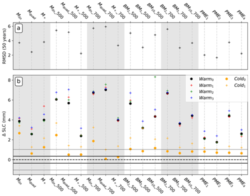
Parameterising sub-shelf melt rates in ice-sheet modelling is currently the only way to account for melting in large-ensemble or multi-millennium simulations of the Antarctic ice sheet (DeConto and Pollard, 2016), and even shorter term simulations applied to single Antarctic basins have been done on very few occasions and only very recently (Thoma et al., 2015; Seroussi et al., 2017). Our study suggests that parameterisations should be chosen with caution. To assess the capacity of the parameterisations to reproduce the ocean-induced melting and its effect on ice-sheet dynamics under a wide range of scenarios, we set-up a performance indicator (Fig. 9). We define it as the root-mean-square deviation (RMSD) in SLC of every parameterisation with respect to the average of coupled simulations on a given year. We choose to calculate this performance indicator at the 50th year of the simulations, for a significant part of the ice shelf is melted out by the parameterisations after this year.

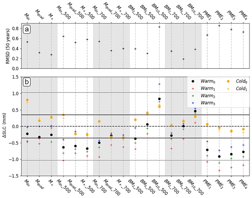
Figure 9 Performance of parameterisations compared to coupled simulations, calculated at the 50th year of simulations. (a) Root mean square deviation (RMSD) in SLC of every parameterised simulation with respect to the average of coupled simulations. (b) Difference between SLCs from parameterisations and coupled simulations for all the experiments. The grey shading is only to ease the comparisons between the parameterisations.

While the plume parameterisation is in pretty good agreement with coupled simulations for the cold forcings, it consistently underestimates both the melt rates and subsequent SLC for the warm forcings. Lazeroms et al. (2018) show melt rate patterns in good agreement with observations for the large ice shelves such as Ronne-Filchner and Ross. However, for smaller ice shelves such as the Pine Island and Thwaites glaciers, the patterns exhibit very strong melting near the calving front, and quite a uniform melting in the entire cavity. This is contradictory to observation-based estimates (Rignot et al., 2013a; Dutrieux et al., 2013) and to high-resolution ocean simulations (Dutrieux et al., 2014) showing large melt rates near the grounding line that drop abruptly from a few kilometres downstream to almost zero near the calving front. In our plume parameterisation configuration, the melt rates are zero at the grounding line, close to zero nearby (not seen in the Lazeroms et al., 2018, paper because the resolution is too coarse) and the strongest at the calving front. We suspect this is due to the empirical relationship used in Lazeroms et al. (2018) that relates melt rates to the depth difference between the effective grounding line point and the ice draft, which may wrongly place the melting–accretion point for small ice shelves as opposed to large ice shelves. The fact that the same ice-sheet response occurs regardless of the type of implementation supports this point.

The box parameterisation tends to give relatively good results regardless of the number of boxes or the near sea-floor depth at which the ocean properties are taken. Using five boxes seems to yield the best results. Reese et al. (2018a) found that increasing the number of boxes in a static cavity would converge to almost constant average melt rates above five boxes. In our study, increasing the number of boxes leads neither to convergence of the calibrated parameter nor to converging SLC during the prognostic simulations. The melting pattern has an effect on the ice-sheet dynamics, so even though convergence could be expected from the work of Reese et al. (2018a) for a static cavity, the ice-sheet response to the different patterns related to the various number of boxes could have suppressed the initial convergence.

A key issue in our implementations of the 1-D plume parameterisation might be in the use of deep ocean temperatures, which will lead to an overestimate of melting near the ice front. Our calibration procedure then scales back the melting near the grounding line and leads to an underestimate of the reduction in buttressing. The box model also uses the deep temperatures, but in that parameterisation heat is supplied to the overturning circulation in the grounding zone only, beyond which melt rates must fall as a result of the extraction of latent heat and the rise in the freezing point. Calibrating the heat transfer coefficient alters the balance between heat used to melt in the grounding zone and that advected downstream to melt elsewhere. Hence, the calibration redistributes the melting rather than just scaling a fixed melt pattern, and that may be the reason that the results compare quite well with those from the coupled model, especially when the parameterisation is used with five boxes.

Among the simple functions of thermal forcing, the two quadratic (local and non-local) functions are in good agreement with the coupled simulations. A non-local dependency leads to slightly better results. Taking the ocean properties at a varying depth gives better results. In that case, these two parameterisations are the only ones to capture the increased melting in coupled simulations after the initial adjustment phase in the Warm₁ scenario. When these simple functions depend on constant depth ocean properties, deeper temperature and salinity inputs result in better agreement with coupled simulations.

We chose to calibrate the parameterisations using the same far-field ocean temperature and salinity constant profiles, which is different from the temperature and salinity scenarios used in the rest of the study. Such an approach is actually very selective but enables to distinguish between parameterisations that could be applied to real cases, because they adapt well to a change in ocean properties, from those that either need to be improved or discarded with regard to changing ocean conditions.

All parameterisations yield too large melt rates in thin ice areas and too small melt rates near the deepest parts around the grounding line. Even though our geometrical set-up is ideal, the distribution of thicknesses within the ice shelf are not far from reality, meaning that applying these parameterisations to real ice shelves would also induce too much thinning of initially thin floating ice. The studies of Jenkins (2016) and Jenkins et al. (2018) suggest that the basal slope of the ice shelf influences the mixing across the thermocline. Accounting for this effect in simple functions of thermal forcing may allow to redistribute more melting over the steep areas near grounding line and less melting over flat areas near calving fronts, thus decreasing the overmelting of thin floating ice.

The choice of a parameterisation for real applications may account for the local circulation in the ice-shelf cavity. Whether the circulation is horizontal or vertical may guide the choice of the dependence on thermal forcing being either a function of varying depth or taken at a constant depth. For instance, the circulation in the Amundsen sea embayment appears to be a mix between vertical overturning fed by incursions of CDW and horizontal barotropic flow generated by tides (Jourdain et al., 2017, 2018). It should be noted that our study does not account for sea ice, which tends to limit the Ekman pumping due to wind stress and vertical mixing, nor for tides.

The spatial distribution of melt rates affect ice-shelf buttressing in a complicated way. Similar total melt rates distributed differently beneath the ice shelf is likely to induce distinct responses of the ice sheet (Reese et al., 2018b; Gagliardini et al., 2010). Conversely, different melting patterns can induce similar responses of the ice sheet if the integrated losses in buttressing happen to be well balanced from one another. This is illustrated in our simulations, for instance by the two types of quadratic functions of the thermal forcing that exhibit different patterns but lead to similar SLC. The study of Reese et al. (2018b) attributes an equal effect of bits of ice-shelf removal on ice-sheet dynamics in places where ice thicknesses can be very different. Removing floating ice near the deepest grounding lines or near ice rises can remove the same amount of buttressing and lead to similar SLC. Ice rises are generally found in shallow waters, and thus a parameterisation that computes overly large melt rates near this sensitive area may remove too much buttressing restraining the upstream ice sheet compared to coupled simulations.

An ocean–ice-sheet coupled model is needed as a reference to assess the melting parameterisations. Only an ocean model can convey the complexity of ocean physics to melting at the ice-shelf base, as opposed to parameterisations, and only an ice-sheet model can respond to a change in ice-shelf buttressing induced by changing melt rates. On the one hand, the ocean model NEMO was used to calculate the melt rates in the coupled framework. On the other hand, the ice sheet was simulated by the Elmer/Ice model using the SSA* approximation of the Stokes equations and a Schoof friction law at the ice–bed interface. Over the last decade, many ice-sheet and ocean models were developed, which motivated various model intercomparison projects to evaluate the caveats and assets of models and their physics with regard to ideal simulations (the MISMIP and MISMIP3D projects in Pattyn et al., 2012, 2013, for ice-sheet models; the ISOMIP project in Holland et al., 2003, for ice-shelf–ocean models; and the MISMIP+, ISOMIP+, and MISOMIP1 projects in Asay-Davis et al., 2016, for ice sheet, ice-shelf–ocean, and ocean–ice-sheet coupled models). These intercomparison projects have highlighted differences between models that have not been accounted for in our study, even though we included an ensemble of coupled configurations to quantify uncertainties in the ocean model grid and physics. This present study will need to be pursued using other types of models and physics to further assess the robustness of our results.

Our study highlights the assets and caveat of sub-shelf melt parameterisations that can be constrained by the far-field ocean, some of which are used over a decade without thorough assessment. This work was performed with an idealised representation of a relatively small outlet glacier in West Antarctica and now needs to be extended to Antarctic realistic ocean–ice-sheet systems in order to improve sea level projections.

6 Conclusions

We compared a wide variety of sub-shelf melting parameterisations depending on oceanic properties to an ensemble of ocean–ice-sheet coupled simulations, using a new coupled model combining the ocean model NEMO and the ice-sheet model Elmer/Ice. Among the complex parameterisations that we assessed, representing melting through a 2-D emulation of a 1-D plume model gives good results for cold conditions (e.g. in the Ronne-Filchner cavity) but underestimates the melt rates and sea level contribution for warm conditions (e.g. in Pine Island glacier cavity). Given the high degree of complexity in the physics represented in the plume model, it is possible that calibrating more parameters could improve the validity of the scaling across multiple ice-shelf sizes. More work may also improve the way to extend the 1-D plume model to a realistic ice draft. The box parameterisation representing the vertical overturning in the cavity gives results relatively close to the coupled simulations, especially when used with five boxes. We showed that a linear parameterisation of thermal forcing is not able to represent ocean-induced melting beneath an ice shelf. Instead, a quadratic parameterisation of thermal forcing gives much better results, which are even improved for a local and non-local approach, as opposed to a fully local approach. Studies aiming at projecting the future contribution of Antarctica to sea level should take care about the choice of the melting parameterisation before providing predictions. We recommend validating the chosen parameterisation with regard to ocean–ice-sheet model coupled simulations within the specific environmental conditions and ice physics, although our results have to be taken carefully, until assessment based upon other models are produced.

Appendix A: Schoof friction law

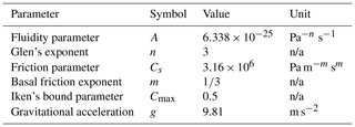
The Glen's flow law relates deviatoric stresses τ_ij to strain rates ${\dot{\mathit{\epsilon }}}_{ij}$ as follows:

$$\begin{array}{}\text{(A1)}& {\mathit{\tau }}_{ij}=A^{-\mathrm{1}/n}{\dot{\mathit{\epsilon }}}_e^{(\mathrm{1}-n)/n}{\dot{\mathit{\epsilon }}}_{ij},\end{array}$$

with A the fluidity parameter, ${\dot{\mathit{\epsilon }}}_e$ the second invariant of strain rates, and n Glen's exponent.

The Schoof friction law is written as in Brondex et al. (2017) and Brondex et al. (2018) as follows:

$$\begin{array}{}\text{(A2)}& {\mathit{\tau }}_{\mathrm{b}}={\displaystyle \frac{C_s{u}_{\mathrm{b}}^m}{{\left(\mathrm{1}+{\left(\frac{C_s}{C_{max}N}\right)}^{\mathrm{1}/m}{u}_{\mathrm{b}}\right)}^m}},\end{array}$$

with τ_b the basal friction, C_s a friction parameter, u_b the basal velocity, C_max Iken's bound parameter, N the effective pressure, and m the basal friction exponent.

The values of the parameters accounted for in Eqs. (A1) and (A2) are given in Table A1.

Table A1 Parameters of Glen's flow law and Schoof friction law. n/a – not applicable

Appendix B: Sensitivity to the coupling period

.

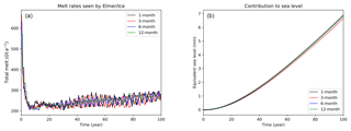
Figure B1 Mean cavity melt rate seen by Elmer/Ice for various coupling periods (a). Global mean sea level rise equivalent to the ice-mass loss simulated by Elmer/Ice for various coupling periods (b). The four simulations correspond to the IceOcean1r experiment of the standard MISOMIP protocol (Asay-Davis et al., 2016).

Appendix C: Physical basis for the plume parameterisation empirical scaling

The plume parameterisation is derived empirically from the results of a full plume model (Jenkins, 2014) applied to a range of simple ice-shelf geometries and water properties. If the ice-shelf base is linear and the far-field ocean uniform, results for a wide range of ocean temperatures, ice-shelf basal slopes, and grounding-line depths, when appropriately scaled, collapse (within ±20 %) onto a universal melt rate curve (Jenkins, 2014). The plume parameterisation of Lazeroms et al. (2018) was created by fitting an 11th-order polynomial function to the universal curve.

When applying the parameterisation in practice, there are a number of issues to deal with: the ice-shelf basal slope will vary; the far-field ocean will be non-uniform; and for 2-D ice-shelf geometries, there is no unique grounding-line point. The first two are generic problems that arise from the simplifications that are required to allow the derivation of a universal melt rate curve. The latter arises when the 1-D parameterisation is implemented in 2-D.

The ice shelf basal slope θ enters the parameterisation through the following function:

$$\begin{array}{ll}{\displaystyle }g\left(\mathit{\theta }\right)=& {\displaystyle }{\left({\displaystyle \frac{\sin \mathit{\theta }}{C_{\mathrm{d}}{E}_{\mathrm{0}}\sin \mathit{\theta }}}\right)}^{\mathrm{1}/\mathrm{2}}{\left({\displaystyle \frac{C_{\mathrm{d}}^{\mathrm{1}/\mathrm{2}}{\mathrm{\Gamma }}_{\mathrm{TS}}}{C_{\mathrm{d}}^{\mathrm{1}/\mathrm{2}}{\mathrm{\Gamma }}_{\mathrm{TS}}+E_{\mathrm{0}}\sin \mathit{\theta }}}\right)}^{\mathrm{1}/\mathrm{2}}\\ \text{(C1)}& {\displaystyle }& {\displaystyle }\left({\displaystyle \frac{E_{\mathrm{0}}\sin \mathit{\theta }}{C_{\mathrm{d}}^{\mathrm{1}/\mathrm{2}}{\mathrm{\Gamma }}_{\mathrm{TS}}+E_{\mathrm{0}}\sin \mathit{\theta }}}\right).\end{array}$$

The last of these terms scales the thermal driving in the plume as a fraction of the far-field thermal driving, while the first two scale the plume speed based on the balance between buoyancy and friction (first) and the dependence of the buoyancy on far-field thermal driving (second). Since the inertia of the plume is small, its speed rapidly adjusts to changing slope, and the first term of the above expression therefore represents a local balance between the upslope buoyancy force and frictional drag. The latter two terms, on the other hand, reflect the balance between entrainment and melting over the path of the plume, and so cannot be directly related to the local slope, if the slope is non-uniform. However, for low slopes the turbulent transfer of heat and momentum at the ice base tends to dominate over entrainment, giving the following:

$$\begin{array}{}\text{(C2)}& g\left(\mathit{\theta }\right)={\left({\displaystyle \frac{\sin \mathit{\theta }}{C_{\mathrm{d}}}}\right)}^{\mathrm{1}/\mathrm{2}}\left({\displaystyle \frac{E_{\mathrm{0}}\sin \mathit{\theta }}{C_{\mathrm{d}}{\mathrm{\Gamma }}_{\mathrm{TS}}}}\right).\end{array}$$

Hence, for low slopes the thermal driving evolves along the plume path with a simple sin θ scaling that effectively makes it a function of the depth change between the grounding line and the point of interest. It does not matter if that path is short and steep with rapid entrainment, or long and gentle with slow entrainment; the net result is the same. The first term remains a local scaling, so when the parameterisation is applied to 1-D problems with varying slope, using the local slope to estimate g(θ) gives good results (Lazeroms et al., 2018).

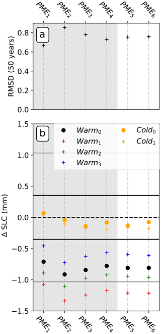
Figure C1 Similar to Fig. 9 but to evaluate the use of the local gradient in PME₃ (which gives PME₅) and PME₄ (which gives PME₆) to calculate the effective angle instead of using the slope between the ice draft and the grounding line from which the plume starts. The calibration of PME₅ and PME₆ is done with α=0.34 and α=0.65, respectively (Sect. 3.2). The grey shading is only to ease the comparisons between the parameterisations.

An equivalent solution to the problem of non-uniform far-field properties is less obvious. Taking a depth-average to reflect the range of properties entrained into the plume is the option used in Lazeroms et al. (2018). However, entrainment is strongest where the basal slope is steepest, so we might expect deeper waters to contribute more to the plume. In this study, we use the temperature at the depth of the grounding line. Since the temperature profiles all have a thick isothermal layer at the seabed, taking an average over the depth range from which waters are entrained into the plume would probably yield similar results, because the isothermal layer would dominate.

Implementation of the plume parameterisation in 2-D is a more complex problem, to which there are many possible solutions. The procedure implemented by Lazeroms et al. (2018) was effectively an average of 1-D implementations along whichever of 16 prescribed directions represented valid plume paths. For each valid direction the grounding-line depth and the local slope in that direction were used to scale the melt rates. In PME₁ we implemented that procedure as closely as possible, given the unstructured model grid (Appendix D). However, following the above reasoning, it could be argued that the path followed by the plume should not matter. Only the depth change from the grounding line to the point of interest should influence the results, and the plume should flow locally up the steepest slope, i.e. parallel to the gradient vector. Using the magnitude of the local gradient vector as the slope scale (PME₂) decreases the checkerboard noise in the PME₁ melt rates (Fig. 4) but does not greatly influence the results. In PME₃ and PME₄, we adopted two procedures for picking a unique grounding line point for each grid point, rather than using an average of many. In each case, we scaled the melt rate using the depth of the grounding-line point and the mean slope along a straight line connecting the grounding line point and the grid point. Following the earlier reasoning, using the magnitude of the local gradient vector is equally valid. Results using that alternative are shown in Fig. C1 but differ little from those presented in Fig. 9.

Appendix D: Implementations of the plume parameterisation in Elmer/Ice

The plume parameterisation was originally implemented for regular grids. We adapt the method used to calculate the effective grounding line depth and effective angle as defined in Lazeroms et al. (2018) to the unstructured grids used in Elmer/Ice. Here, we describe the adapted method and the alternative implementations also discussed in the paper.

D1 PME₁ (plume model emulator 1)

In the original algorithm published in Lazeroms et al. (2018), the melt rates at a draft point are calculated by considering the effective grounding line depth, which is calculated by searching in the 16 grid directions equally distributed around the draft point, and starting from it, insofar as those directions are valid. The 16 directions follow the grid points as shown in Fig. 3 of Lazeroms et al. (2018). A direction is valid if (i) the local slope in this direction is negative and (ii) the first grounded point met in this direction is deeper than the draft point in this direction. The effective grounding-line depth of the draft point (i,j) of the regular grid z_gl(i,j) is calculated using Eq. (13a) of Lazeroms et al. (2018), and its effective angle θ(i,j) is calculated using Eq. (13b) by considering the local slopes in the valid directions. These equations are recalled here below:

$$\begin{array}{}\text{(D1)}& {\displaystyle }& {\displaystyle }{z}_{\mathrm{gl}}(i,j)={\displaystyle \frac{\mathrm{1}}{N_{ij}}}\sum _{\mathrm{valid}n}{z}_n(i,j),\text{(D2)}& {\displaystyle }& {\displaystyle }\tan \left[\mathit{\theta }\right(i,j\left)\right]={\displaystyle \frac{\mathrm{1}}{N_{ij}}}\sum _{\mathrm{valid}n}{s}_n(i,j),\end{array}$$

with N_ij the number of valid directions, z_n(i,j) the grounding line depth, and s_n(i,j) the local slope in the direction of the grounding line.

Instead of grid directions, we consider directional triangles that are angularly equally distributed around the draft point. Analogously to the original criterion to find valid directions, the criterion to make a cone valid is based on (i) the average of the local angles of all the directions connecting the draft point to the grounding line points included in the cone and (ii) the average of these grounding line point depths (Fig. D1a). The simulations were all done using 64 triangles around the draft point, which enables a rather smooth melting pattern compared to using 16 triangles (analogously to Lazeroms et al., 2018, for directions).

D2 PME₂

In the algorithm published in Appendix 2 of Lazeroms et al. (2018), i.e. the discussion version of Lazeroms et al. (2018), the criterion to make a direction valid is the same as the first algorithm, but the computation of the effective grounding-line depth and angle is slightly different, taking for instance the local gradient instead of the local slope in each direction to calculate the effective angle.

We calculate the effective grounding line depth and angle as it is in Eqs. (B1) and (B2) of Lazeroms et al. (2018) but using the search for valid directions as explained in Sect. D1 (Fig. D1a), also using 64 triangles.

D3 PME₃

In this algorithm, we simply take the deepest grounding line (which is located in the central flow line) to calculate the effective grounding line depth, and the effective angle is the slope between this grounding-line point and the draft point (Fig. D1b).

D4 PME₄

This algorithm accounts for the asymmetry resulting from the Coriolis effect, although in a very crude manner. The effective grounding-line depth is found by starting from the closest grounding-line point and looking for a deeper contiguous grounding-line point in the anti-clockwise direction as long as the grounding line deepens. Two examples of this algorithm are shown in (Fig. D1c) for two draft points in the left and the right side of the cavity, respectively. The effective angle is calculated as in Appendix D3.

D5 PME₅

This implementation is similar to PME₃ but the effective angle is calculated from the ice-draft local gradient. The results are not given in the main article but compared to the other plume parameterisations in Fig. C1.

D6 PME₆

This implementation is similar to PME₄ but the effective angle is calculated from the ice-draft local gradient. The results are not given in the main article but compared to the other plume parameterisations in Fig. C1.

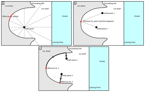
Figure D1 Computing the effective grounding-line depth and angle for the four plume parameterisation implementations. Panel (a) illustrates both the published implementation PME₁ (Lazeroms et al., 2018) and the one appearing in the corresponding discussion article PME₂ (Lazeroms et al., 2018), here with 12 directions (vs. 64 triangles used in the present paper). PME₁ and PME₂ differ by the calculation of the effective slope, which is not depicted here. Panel (b) illustrates the simple implementation PME₃ and panel (c) illustrates the asymmetric implementation PME₄.

Appendix E: CMIP5 temperature anomalies in the Amundsen Sea under the RCP8.5 scenario

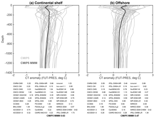
Figure E1 Temperature anomaly (2080–2100 mean minus 1989–2009 mean) in the Amundsen Sea (76–69^∘ S, 128–90^∘ W) from 33 CMIP5 models in the RCP85 scenario. Continental shelf temperatures (a) are averaged over the area where the sea floor is shallower than 1500 m, while offshore temperatures (b) are averaged over the rest of the domain. The numbers for individual CMIP5 models and the multi-model mean (MMM) indicate the mean ocean warming in the 500–800 m layer.

Appendix F: MISOMIP original calibration below 300 m depth

Figure F1 Same as Fig. 9 but for an initial calibration based on averaged melt rates below 300 m depth.