the Creative Commons Attribution 4.0 License.
the Creative Commons Attribution 4.0 License.
 | 07 Jun 2019
Description and validation of an intermediate complexity model for ecosystem photosynthesis and evapotranspiration: ACM-GPP-ETv1
Thomas Luke Smallman
Mathew Williams
Photosynthesis (gross primary production, GPP) and evapotranspiration (ET) are ecosystem processes with global significance for climate, the global carbon and hydrological cycles and a range of ecosystem services. The mechanisms governing these processes are complex but well understood. There is strong coupling between these processes, mediated directly by stomatal conductance and indirectly by root zone soil moisture content and its accessibility. This coupling must be effectively modelled for robust predictions of earth system responses to global change. Yet, it is highly demanding to model leaf and cellular processes, like stomatal conductance or electron transport, with response times of minutes, over decadal and global domains. Computational demand means models resolving this level of complexity cannot be easily evaluated for their parameter sensitivity nor calibrated using earth observation information through data assimilation approaches requiring large ensembles. To overcome these challenges, here we describe a coupled photosynthesis evapotranspiration model of intermediate complexity. The model reduces computational load and parameter numbers by operating at canopy scale and daily time step. Through the inclusion of simplified representation of key process interactions, it retains sensitivity to variation in climate, leaf traits, soil states and atmospheric CO2. The new model is calibrated to match the biophysical responses of a complex terrestrial ecosystem model (TEM) of GPP and ET through a Bayesian model–data fusion framework. The calibrated ACM-GPP-ET generates unbiased estimates of TEM GPP and ET and captures 80 %–95 % of the sensitivity of carbon and water fluxes by the complex TEM. The ACM-GPP-ET model operates 3 orders faster than the complex TEM. Independent evaluation of ACM-GPP-ET at FLUXNET sites, using a single global parameterisation, shows good agreement, with typical R2∼0.60 for both GPP and ET. This intermediate complexity modelling approach allows full Monte Carlo-based quantification of model parameter and structural uncertainties and global-scale sensitivity analyses for these processes and is fast enough for use within terrestrial ecosystem model–data fusion frameworks requiring large ensembles.
- Article
(4557 KB) - Full-text XML
- BibTeX
- EndNote


Ecosystem photosynthesis and evaporation are key ecosystem fluxes, and their strong coupling generates important feedbacks between plant carbon and water cycles (Tuzet et al., 2003; Bonan and Doney, 2018). Ecosystem photosynthesis, or gross primary productivity (GPP), is generally the sole input of organic carbon into terrestrial ecosystems, ultimately determining potential carbon accumulation rates. Ecosystem evaporation, or evapotranspiration (ET), is the combination of plant-mediated transpiration, soil surface evaporation and subsequent evaporation of rainfall intercepted by plant canopies. The dominant abiotic factors governing the magnitude and variability of GPP are temperature, absorbed photosynthetically active radiation (PAR) and CO2, which are strongly impacted by leaf area index (LAI). Access to CO2 is controlled via leaf stomata, which provide the primary coupling point between GPP and the water cycle. Stomatal opening results in water loss via transpiration, creating a dependency on accessible soil moisture, which is controlled by root biomass and its distribution through the soil profile. Thus, the soil–root interface is a second coupling point between the plant carbon and water cycles (Beer et al., 2009; Bonan and Doney, 2018). State-of-the-art terrestrial ecosystem models (TEMs) provide a mechanistic and process-oriented representation of the coupling between plant carbon and water cycles (e.g. Krinner et al., 2005; Oleson et al., 2010; Smallman et al., 2013; Harper et al., 2016) at leaf or even sub-leaf scale, resolving radiative transfer, stomatal conductance and electron transport. TEMs represent state-of-the-art knowledge on how ecosystems function and are used to provide meaningful predictions of the responses by and feedbacks from the terrestrial land surface in response to changes in the earth system (Bonan and Doney, 2018). Mechanistic models linking leaf-level photosynthesis (e.g. Farquhar and von Caemmerer, 1982; Collatz et al., 1991) and transpiration (e.g. Monteith, 1965) through models of stomatal regulation (Medlyn et al., 2011; Williams et al., 1996; Bonan et al., 2014) are well established. Scaling from leaf to canopy scale has grown increasingly complex as the role of non-linear within-canopy variation of both abiotic (e.g. light, temperature, momentum, CO2 and H2O) and biotic (i.e. plant traits) factors in plant carbon–water relations has improved (e.g. Wang and Leuning, 1998; Buckley et al., 2013; Sun et al., 2014; Way et al., 2015; Coble et al., 2016; Scartazza et al., 2016; Nolan et al., 2017; Bonan et al., 2018).
However, the increasing complexity of TEMs presents new challenges. Many of the most complex TEMs are too slow for use in model–data fusion analyses, which are reliant on massive ensemble simulations (e.g. Ziehn et al., 2012; Smallman et al., 2017). While effective and more computationally efficient alternative model–data fusion approaches are available, they often rely on model code modifications, such as the creation of the model adjoint in variational approaches (e.g. Kuppel et al., 2012; Raoult et al., 2016) or model emulation, often resulting in larger uncertainties in their posterior analysis (e.g. Fer et al., 2018). The complexity of typical TEMs generally prevents a robust quantification of their uncertainties; it is very challenging computationally to determine the sensitivities of TEM model outputs to parameter variation. This hinders interpretation of model–data mismatch. Finally, there are major challenges in procuring sub-daily meteorological observations needed to drive TEMs away from meteorological stations – this is a particularly acute problem in tropical regions. Thus, TEMs are generally run using statistical downscaled climate reanalysis data, which contain errors. The uncertainty generated when these errors are propagated into TEM GPP and ET estimates is comparable to intermediate complexity (IC) model error associated with simulating daily fluxes directly (Williams et al., 1997, 2001a). Thus, IC models have been shown to have similar errors to TEM models but at lower computational cost (i.e. 1 time step versus 24 time steps). Thus, there is considerable value in having less complex, fast-running models that simulate GPP and ET. The challenge here is to produce a model both sufficiently mechanistic to represent the coupling between plant carbon and water cycles linking to ecophysiological processes and observations of key global unknowns (e.g. rooting depth) but also computationally fast enough to be integrated into model–data fusion schemes and to allow a full exploration of parameter-related uncertainties.
Photosynthesis is often estimated using physiologically realistic light, CO2 and temperature response functions (e.g. Jones, 1992; Williams et al., 1997). Evaporation is frequently estimated using simplified versions of the Penman–Monteith model, typically modelling plant stomatal regulation as a function of environmental drivers (e.g. Priestley and Taylor, 1972; Fisher et al., 2008). The impact of moisture limitations on both GPP and ET is commonly achieved through the use of the vapour pressure deficit (VPD) as a proxy (e.g. Mu et al., 2011; Wang et al., 2017) or using a single soil layer “bucket” (e.g. Martens et al., 2017). While simple models can show skill when compared to in situ estimates (Mu et al., 2011; Bloom and Williams, 2015; Martens et al., 2017; Wang et al., 2017), they usually estimate a single process, either photosynthesis or evapotranspiration, neglecting their coupling. Without coupling, the feedbacks between C and water cycles will not be modelled robustly. For instance, there is a high risk that independently calibrated, simple GPP and ET models that are coupled naively in a plant–soil model framework will misdiagnose the sensitivity of water use efficiency (C fixed per water transpired) and have low predictive capability outside of the calibrated range (e.g. big leaf versus multiple leaf canopy; Tuzet et al., 2003; Wang and Leuning, 1998). Thus, connecting a series of simple models to generate a model of IC carries significant risks. The IC model must represent process interactions effectively. A key test therefore is that any IC model must reproduce the sensitivities of key processes (i.e. GPP, ET), their interactions (WUE) and soil moisture status demonstrated by the state-of-the-art TEMs to ensure flux estimates are right for the right reasons.
This study builds on two previously developed aggregated canopy models (ACMs) for GPP (Williams et al., 1997) and ET (Fisher et al., 2008) and an existing state-of-the-art TEM, Soil Plant Atmosphere (SPA; Williams et al., 1996; Smallman et al., 2013). ACM-GPP simulated daily GPP sensitive to canopy nitrogen (N), temperature, absorbed short-wave radiation and atmospheric CO2 concentration, based on physiologically realistic relationships but lacking a representation of the impact of soil moisture availability on photosynthesis. Despite this limitation ACM-GPP has been coupled to the DALEC C-cycle model (Williams et al., 2005) and successfully used in model–data fusion experiments to improve our understanding of ecosystem C status, C allocation and residence times (Fox et al., 2009; Bloom and Williams, 2015; Bloom et al., 2016; Smallman et al., 2017) but also carbon–nitrogen interactions (Thomas and Williams, 2014). In addition to lacking a soil moisture response to photosynthesis, ACM-GPP limits the capacity of DALEC analyses to constrain the root component of the C cycle as roots currently play no ecological role within the modelling system (i.e. water or nutrient uptake). ACM-ET simulates the bulk ecosystem evapotranspiration based on a modified Penman–Monteith approach sensitive to absorbed short-wave radiation, temperature, vapour pressure deficit and wind speed. However, ACM-ET's bulk approach does not allow for distinguishing between different evaporative sources (i.e. soil surface, root-extracted rainfall and canopy-intercepted rainfall). Thus, it does not account for the different biotic and abiotic drivers which have varied responses to environmental change (Wei et al., 2017). Moreover, ACM-ET does not have a mechanistic coupling to water supply governed by root biomass and root vertical distribution. ACM-GPP and ACM-ET use different empirical models linking LAI, minimum tolerated leaf water potential and meteorological drivers to estimate canopy conductance. Both ACMs can be calibrated to provide useful GPP and ET estimates; however when combined their predictive capacity for emergent properties such as WUE is limited (R2<0.2; data not shown), highlighting the need for further development to reproduce emergent ecosystem properties.
Here we describe a process model of intermediate complexity, ACM-GPP-ET version 1, that simulates gross primary productivity and evapotranspiration. ACM-GPP-ET is a fast, coupled representation of plant carbon and water cycles at ecosystem scale and daily time resolution. Coupling is achieved via a canopy stomatal model that determines CO2 and H2O exchanges in the canopy. With fewer parameters than many state-of-the-art process-orientated models, our model is simpler to calibrate. With a daily time step and single canopy layer, the model is fast and therefore viable for ensemble modelling. In fact ACM-GPP-ET is explicitly intended as a replacement for ACM-GPP as part of the DALEC model, addressing current weaknesses in simulating carbon–water interactions with our model–data fusion framework. To ensure its realism, ACM-GPP-ET is an emulation of a more complex TEM, SPA (Williams et al., 1996), that resolves leaf-scale, hourly exchanges of CO2 and water. SPA also includes a detailed, multi-layer representation of radiative transfer, energy balance, carboxylation and plant–soil interactions at sub-daily timescales. SPA explicitly couples available supply of water from the soil (determined as a function of soil characteristics, root biomass and structure) to demand by the atmosphere (as a function of absorbed radiation and vapour pressure deficit) which results in robust dynamics in response to varied water availability (Bonan et al., 2014). We create a very large ensemble of SPA runs across environmental space to map the sensitivity of GPP and ET to biophysical changes and then fit the parameters of ACM-GPP-ET to these surfaces.
ACM-GPP-ET is based on previous approaches developed to estimate GPP and ET independently (Williams et al., 1997; Fisher et al., 2008) but here uniquely are realistically coupled for the first time. GPP is estimated as a function of foliar nitrogen content allocated to photosynthetic activity, temperature, intercellular CO2 concentration and absorbed PAR. ET is estimated as the sum of transpiration, evaporation from the soil surface and of rainfall intercepted by the canopy, within a soil water mass-balanced system. Using a combination of GPP and ET estimates from both TEM and observation-orientated analyses, spanning site to global scales, we calibrate and validate ACM-GPP-ET and address the following questions:
-
How computationally efficient is ACM-GPP-ET compared to our complex TEM at estimating daily fluxes?
-
How well can the intermediate complexity ACM-GPP-ET emulate the complex TEM (i.e. GPP and ET and their coupling via WUE and soil moisture)?
-
How do ACM-GPP-ET predictions compare to fully independent FLUXNET-derived estimates of carbon and water fluxes across the globe?
Finally we discuss novel research applications made possible using our intermediate complexity, ecophysiologically based modelling approach including full Monte Carlo-based quantification of model parameter and structural uncertainties, global-scale sensitivity analyses (e.g. WUE response to increased CO2), rapid testing of alternative theoretical models of stomatal conductance and use within terrestrial ecosystem model–data fusion frameworks.
2.1 Model overview
The aggregated canopy model for gross primary productivity and evapotranspiration version 1 (ACM-GPP-ET v1) provides a computationally efficient yet broadly mechanistic representation of photosynthetic and evaporative fluxes of terrestrial ecosystems. Evapotranspiration is explicitly represented as the sum of transpiration (coupled to GPP via a mechanistic representation of stomatal conductance), evaporation from the soil surface and evaporation of precipitation intercepted by the canopy. Absorption and reflectance of short- and long-wave radiation are estimated as non-linear functions of LAI. Aerodynamic conductance for canopy and soil surface exchange is estimated as a function of wind speed and canopy structure (LAI and height). ACM-GPP-ET includes a four-layer model of soil water balance. The top three soil layers are accessible to roots, which determines the available supply of water to the plant as a function of fine root biomass and their distribution through the soil profile. Soil evaporation is assumed to be supported by the top soil layer only (Fig. 1).
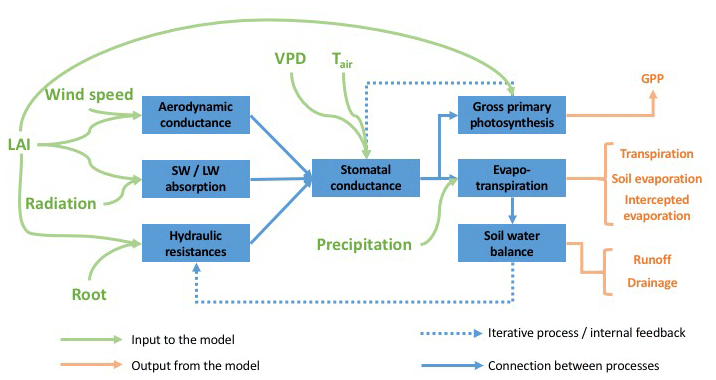
Figure 1Schematic of ACM-GPP-ET showing its inputs, outputs and how its processes are interconnected. The blue boxes indicate distinct process groupings within the model framework. Green arrows are inputs to the model, while orange arrows indicate model output (i.e. carbon and water fluxes). Blue arrows show the interconnections between the various processes.
2.2 Model drivers
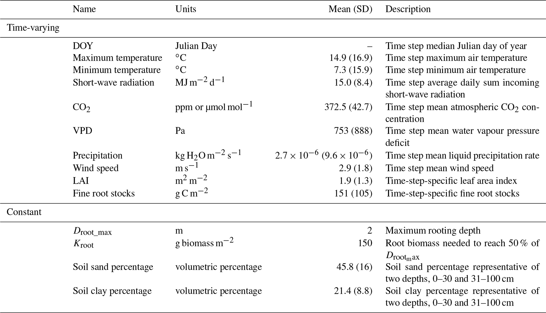
ACM-GPP-ET requires both meteorological and biophysical information as inputs (Table 1). Most of the needed drivers are widely available from either field observations or global reanalyses. Meteorological drivers are extracted from the European Centre for Medium-Range Weather Forecasts (ECMWF) ERA-Interim reanalysis (Dee et al., 2011), while soil textural information is extracted from global interpolations of field inventories (e.g. Harmonized World Soils Database, HWSD; Hiederer and Köchy, 2011). LAI is widely available from satellite-based remote sensing such as the NASA-generated MODIS product (https://modis.gsfc.nasa.gov/data/dataprod/mod15.php, last access: 18 October 2017). In contrast, information on below-ground biophysical information, such as root stocks and rooting depth, is more challenging to obtain as it is highly spatially variable and not directly observable from space. Simulation models and model–data fusion-based C-cycle analyses may simulate root stocks which can provide useful information (e.g. Bloom et al., 2016), while rooting depth information can also be statistically estimated (e.g. Fan et al., 2017).
Table 1Drivers required as inputs by ACM-GPP-ET. Each driver has its unit specified and a brief description. The mean value across the calibration climate space is given with the standard deviation in parentheses. The drivers are divided between those which are time-varying and those assumed constant for a given location but that can vary between locations.
2.3 Model parameters
Parameters within ACM-GPP-ET represent a wide range of time-invariant physical, biogeophysical and biogeochemical properties. In this study we calibrate a total of 22 parameters related to nitrogen-use and light-use efficiency, temperature response of photosynthesis, plant water-use efficiency and radiation absorption and reflectance processes (Table 2); these parameters broadly relate to ecosystem traits. Ecosystem traits can be reasonably expected to vary between ecosystems, and thus we should be able to retrieve ecologically consistent estimates for these parameters given suitable carbon and water flux information. In this study were we are calibrating against a complex model with “known” parameter values against which we can compare our estimated values. There are a further 12 biophysical parameters which are assumed to be constant and therefore are not retrieved as part of our calibration procedure (Table 3).
Table 2ACM-GPP-ET parameters retrieved using the CARDAMOM model–data fusion system. For each parameter its symbol as used in the code description is given, along with the maximum and minimum values used for the prior ranges, the maximum likelihood estimate retrieved from the posterior distributions, units and a brief description. The SPA column contains the SPA parameter value used in the calibration where a direct equivalent is available. Near-infrared radiation is abbreviated as NIR, photosynthetically active radiation as PAR and long-wave radiation as LW.
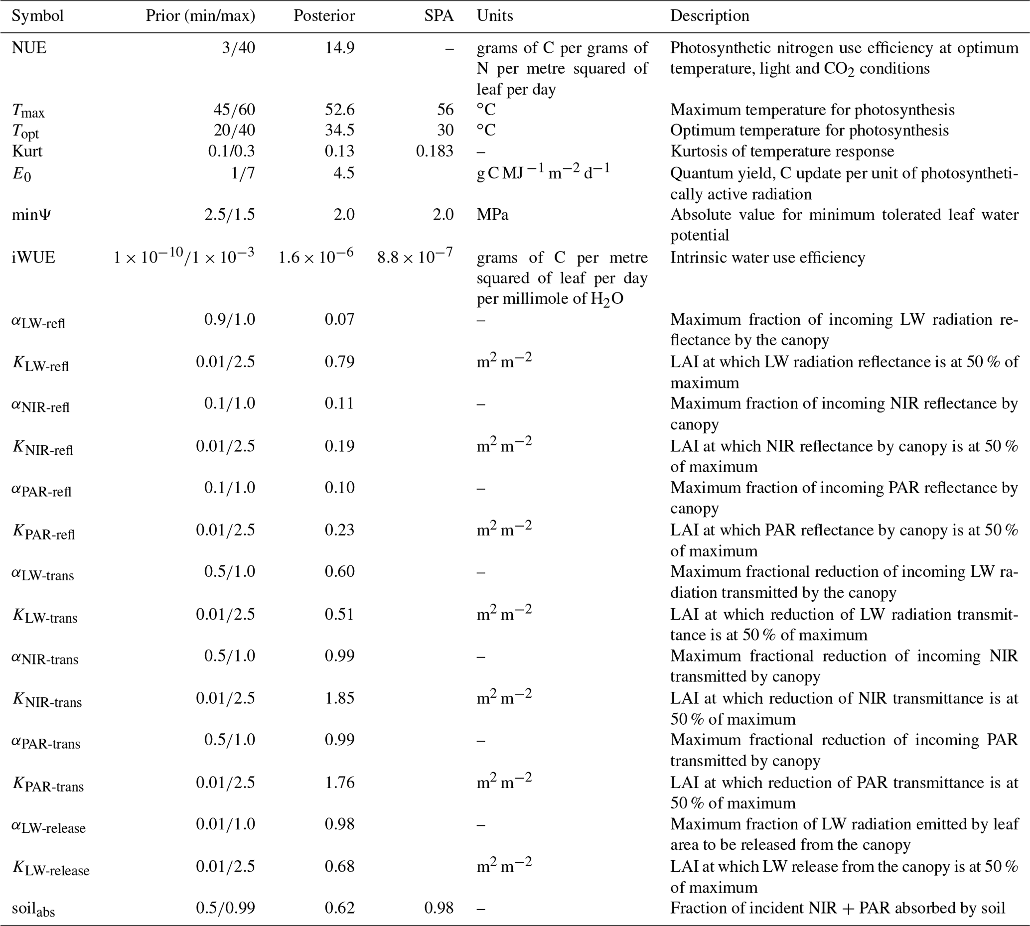
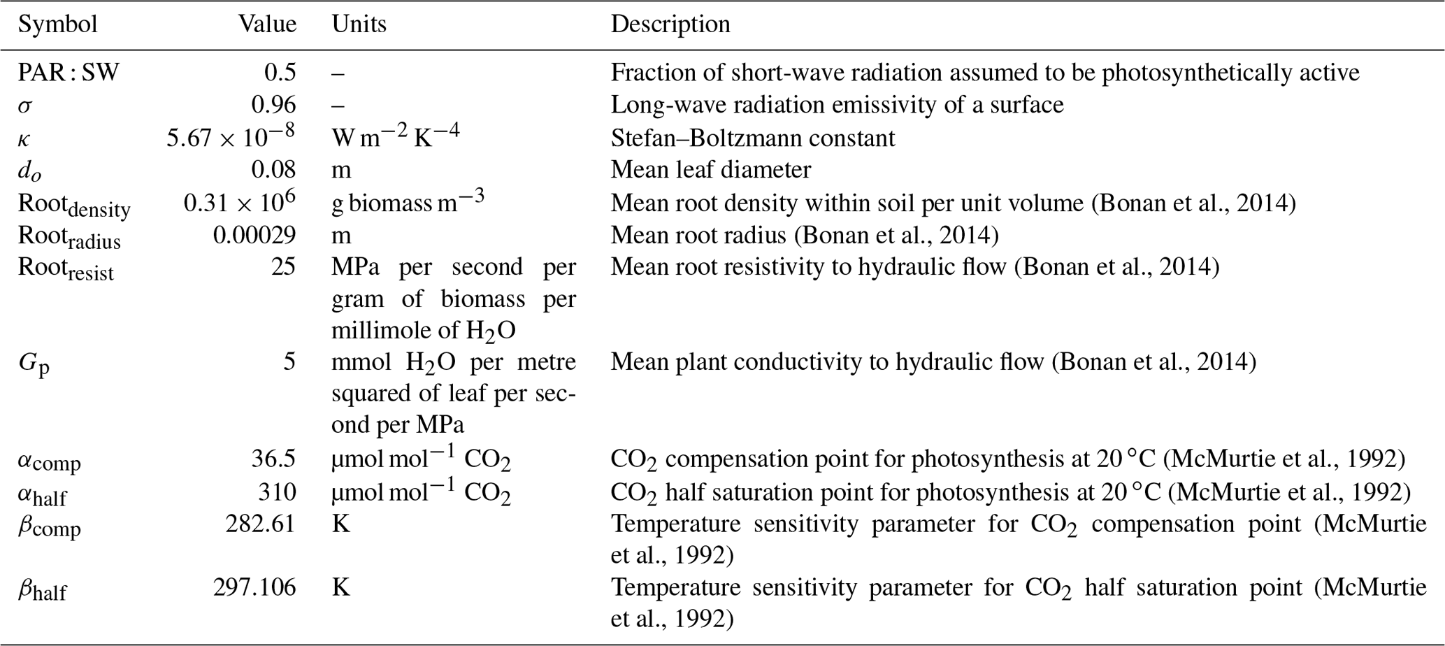
Table 3Parameters describing physical or biophysical constants not retrieved as part of the CARDAMOM model–data fusion analysis.
2.4 Gross primary productivity
Following Williams et al. (1997) and Jones (1992), GPP is estimated as a co-limited function of temperature, CO2 (limited by stomatal opening and thus plant water availability) and absorbed PAR. The temperature- and foliar-nitrogen-limited rate of photosynthesis (PNT; g C m−2 d−1) is first determined as a function of leaf area index (LAI; m2 m−2), average foliage nitrogen content (Nfol; grams of nitrogen per metre squared of leaf), nitrogen use efficiency (NUE; g C/g N/m2 leaf/d) and temperature (Tair; ∘C).
where Tadj describes a skewed normal distribution (scaling 0–1) with an optimum temperature (Topt), maximum temperature (Tmax) and kurtosis (Kurt).
CO2 limitation is dependent on canopy conductance of CO2 (gc; mmolCO2 m−2 d−1), which is assumed to be the combined conductance of the stomata (gs; mmol H2O m−2 s−1) and leaf boundary layer (gb-mmol; mmol H2O m−2 s−1). Note that gs and gb are calculated for conductance of water vapour, and thus coefficients 1.65 and 1.37 convert conductance of water to those of CO2 (Jones, 1992); daylsec=86 400 is the number of seconds per day.
The canopy boundary layer (gb; see Eq. 57) and stomatal conductance (gs) are initially calculated in metres per second (m s−1) and thus must be converted into millimoles of H2O per metre per second (mmol H2O m−2 s−1) for the purposes of calculating CO2 exchange. Note that the coupling between photosynthesis and transpiration occurs via gs, which is estimated as a function of available water supply, atmospheric demand and the intrinsic water use efficiency threshold on GPP; see Sect. 2.6 for details on the estimation of gs.
where TairK is the air temperature in kelvin, Prair is air pressure (default =101 325 Pa) and Rcon is the universal gas constant (8.3144 J K−1 mol−1). The scalar 1000 adjusts units from moles (mol) to millimoles (mmol).
The internal CO2 concentration (Ci; ppm or µmol mol−1) is estimated as a function of atmospheric CO2 concentration (Ca; ppm or µmol mol−1), gc, the CO2 compensation (Ccomp; ppm or µmol mol−1) and half saturation (Chalf; ppm or µmol mol−1) points.
MC (12 g C mol−1) is the molar ratio of carbon, where its inverse ( converts from moles of carbon (mol C) to grams of carbon (g C) and 1×10⁶ scales from micromoles (µmol) to moles.
Ccomp determines the Ci at which GPP becomes positive, while Chalf is the Ci at which CO2-limited photosynthesis is at 50 % of its maximum rate. Both Ccomp and Chalf are calculated as a function of temperature following McMurtie et al. (1992).
where αcomp and αhalf describe the values at the reference temperature (20 ∘C or 298.15 K), and βcomp and βhalf describe the sensitivity of the temperature response.
CO2-limited photosynthesis (; g C m−2 d−1) is calculated as a function of gc and CO2 exchange gradient, where scales from µmol to moles, and MC converts moles to grams of C. At this juncture, a day length (dayl: hours) correction is applied to be consistent with the light limitation calculation which follows
Light-limited photosynthesis (PI; g C m−2 d−1) is defined as a function of absorbed short-wave radiation (I) and a quantum yield parameter (E0).
The final GPP estimate (g C m−2 d−1) is the result of combined light- and CO2-limited photosynthesis.
2.5 Evapotranspiration
Evapotranspiration is based on the Penman–Monteith model assuming isothermal net radiation conditions (Jones, 1992). Evaporation is simulated from three source which are (i) transpiration, (ii) evaporation of precipitation intercepted by the canopy and (iii) the soil surface. The following sections detail the calculation of each evaporative source within their respective available water supplies.
2.5.1 Transpiration
Transpiration (Etrans; kg H2O m−2 d−1) is estimated by the Penman–Monteith equation linking the drivers of transpiration, canopy radiation status and atmospheric demand, with restrictions on evaporative losses, namely available water supply from the roots within the soil profile. The upper limit on water supply is imposed by restricting the maximum stomatal conductance (gs) for a given set of environmental conditions (process described in Sect. 2.6).
where Φiso-canopy is the isothermal net radiation (W m−2; see Sect. 2.7.2), s (kPa K−1) is the slope of curve relating saturation vapour pressure with air temperature and γ is the psychrometer constant (kPa K−1). ρair is the density of air (kg m−3), λ is the latent heat of vaporisation (J kg−1) and cpair is the specific heat capacity of air (J kg K−1). s, γ and λ are calculated as a function of Tair following equations described in Jones (1992).
where sref0 (0.61078 MPa), γref0 (0.0646 kPa) and λref0 (2 501 000 J kg−1) are s, γ and λ at 0 ∘C reference temperature. ρair is calculated as a function of TairK.
The calculation of canopy conductance (gb; m s−1) is described in Sect. 2.8.1 linked to canopy properties (LAI and canopy height) and wind speed. Stomatal conductance (gs; m s−1), used in both the calculation of GPP and transpiration, is calculated via an iterative bisection procedure described in the following section.
2.5.2 Wet canopy evaporation
Wet canopy surface evaporation (Ewet; kg H2O m−2 d−1) is the evaporation of precipitation intercepted by the canopy and thus is limited by the available canopy water storage (Cstor).
where Epot is the potential wet canopy evaporation (kg H2O m−2 d−1). Epot is assumed to be unrestricted evaporation as estimated by the Penman model assuming isothermal net radiation. Epot is further restricted based on the ratio of current canopy water storage:
where Cmax is the maximum canopy water storage (kg H2O m−2), defined as a function of LAI related by α (0.2) as previously used in SPA (Smallman et al., 2013).
where Cstor is determined by water inputs from precipitation, less that which reaches the soil surface (i.e. throughfall) and its water losses by evaporation (as described above) or overflow from intercepted water exceeding Cmax onto the ground. The fraction of precipitation expected to be throughfall (Tfall) is estimated as a function of LAI related by μ (0.5), where μ is selected assuming that interception of rainfall is similar to that of direct radiation.
2.5.3 Soil surface evaporation
Soil evaporation (Esoil; kg H2O m−2 d−1) is estimated using the Penman–Monteith equation linking drivers of evaporation, soil isothermal radiation (Φiso-soil; W m−2) and atmospheric demand, with restrictions on evaporative losses (i.e. available water in the top soil layer). The upper limit of evaporation is also restricted by the thickness of the dry layer (drythick; m) of soil at the surface.
where gsoil is the soil surface aerodynamic conductance (m s−1), and gws is the conductance of water vapour (m s−1) through the soil air space. VPDsoil is the vapour pressure deficit (kPa) between the air above the soil and air within the soil pore space.
where portop is the porosity (0–1; m3 m−3) for the top soil layer as calculated using the Saxton model of soil hydrology (Saxton et al., 1986; Williams et al., 2001b), Dw is the diffusion coefficient for water through air (m2 s−1) at reference temperature 293.2 K and 1.75 is a scalar coefficient relating the temperature dependence of Dw. τ is the tortuosity (i.e. 2.5).
where esurf is the vapour pressure deficit within the soil air space (kPa). esoil is the vapour pressure in the soil air space (kPa), and esat is the saturation vapour pressure at the current temperature. SWPtop is the soil water potential (MPa) for the top soil layer, while Vw is the partial molar volume of water at 20 ∘C (i.e. 1.805 m3 mol−1). All other scalar values are coefficients relating current air temperature to esat.
2.6 Calculating gs: the coupling point between plant C and H2O cycles
The intrinsic water use efficiency (iWUE) optimisation approach for estimating gs is well established and validated; in particular iWUE has been shown to show improved drought response of gs compared to the Ball–Berry gs model (Williams et al., 1996; Bonan et al., 2014). The model aims to maximise photosynthetic uptake within the constraints on gs imposed by the available supply of water to the canopy and atmospheric demand for evaporation; this approach is referred to as optimising the iWUE.
Calculation of gs is a three-step process. Step 1 is the estimation of the potential steady flow water supply over the day (MaxSupply; kg H2O m−2 d−1) from the soil via roots to the canopy.
where LWPmin is the minimum tolerated leaf water potential (MPa), wSWP is the soil water potential weighted by root access (MPa) and Rtot is the total hydraulic resistance (MPa s−1 m−2 mmol−1 H2O). The unit is changed from mmol to kilograms of water (kg H2O) using the molar mass of water (18 g mol−1) and scalar. Step 2 inverts the Penman–Monteith equation to calculate the value of gs required to meet MaxSupply under current atmospheric demand and isothermal net radiation conditions.
Step 3 uses an iterative bisection process which quantifies the sensitivity of GPP to the gs increment by 1 mmol H2O m−2 s−1 (δGPP; grams of C per metre squared of leaf per day per millimole of H2O). The bisection process varies gs between 0 and gs-max minimising gsopt, the difference between δGPP/gs and iWUE, g C/m2 leaf/d/mmol H2Ogs.
2.7 Radiation balance
State-of-the-art radiative transfer schemes are able to quantify differential canopy absorption, transmittance to soil surface and reflection back to the sky of PAR, NIR and long-wave radiation. Using a detailed radiative transfer scheme as a base (Williams et al., 1998), here we have developed simple Michaelis–Menten relationships parameterised to reproduce the emergent absorption, transmittance and reflection properties of a canopy as a function of LAI.
Net canopy (Φiso-canopy; W m−2) and soil (Φiso-soil; W m−2) isothermal radiation balances are calculated from the combination of short- and long-wave absorption detailed in the following sections.
2.7.1 Short-wave radiation absorption
ACM-GPP-ET uses a bidirectional radiative transfer scheme to estimate the absorption of PAR and NIR by the canopy and soil surface. Downward radiation first interacts with the canopy either being reflected back toward the sky, transmitted toward the soil surface or absorbed by the canopy. Second, the radiation which is transmitted through the canopy to the soil surface is either absorbed or reflected back through the canopy.
The fraction of incoming PAR (canopyPAR-abs) and NIR (canopyNIR-abs) absorbed is estimated as the residual of that reflected back into the sky (canopyPAR-refl, canopyNIR-refl) or that transmitted (canopyPAR-trans, canopyNIR-trans) toward the soil surface.
where αNIR-refl and αPAR-refl are the maximum fraction of NIR and PAR reflected by the canopy. KNIR-refl and KPAR-refl are the LAI values at which 50 % of maximum reflectance is achieved for NIR and PAR respectively. αNIR-trans and αPAR-trans are the maximum reduction in transmittance for NIR and PAR; similarly KNIR-trans and KPAR-trans are the LAI at which transmittance is reduced by 50 %. Absorption of PAR (APARcanopy) and NIR (ANIRcanopy) by the canopy on its first pass down through the canopy is estimated as
Transmitted PAR and NIR are then incident on the soil surface to be absorbed by the soil surface or reflected back up towards the canopy. We assume that the soil absorption fraction (soilabs) of incident PAR and NIR is the same; however PAR and NIR remain independently tracked to allow for subsequent reflection back towards the canopy.
PAR and NIR which are reflected from the soil are then available for a second opportunity of the canopy to absorb and typically contributed <1 % of absorbed radiation in ACM-GPP-ET. Therefore the total APARcanopy and ANIRcanopy are calculated as follows:
Estimates of incoming short-wave radiation are widely available; however partitioned estimates of NIR and PAR are less frequent. In such circumstances we assume a fixed ratio between PAR and total short-wave radiation (PAR : SW).
2.7.2 Isothermal long-wave radiation absorption
The long-wave radiation balance is estimated assuming isothermal conditions (i.e. the surfaces are assumed to be the same temperature as the surrounding air). Calculation of the isothermal long-wave radiation is a trade-off between the need to account for a positive bias in available energy for evaporation, should only the short-wave radiation be accounted for, and errors introduced by not considering thermal heating and cooling of surfaces.
Similar to the short-wave radiative transfer scheme described above, ACM-GPP-ET uses a bidirectional radiative transfer scheme to estimate the absorption and emission of long-wave radiation by the canopy and soil surface. The long-wave radiation balance is divided into four components. First, incoming radiation interacts with the canopy either being reflected back toward the sky, transmitted toward the soil surface or absorbed by the canopy. Second, the radiation which is transmitted through the canopy to the soil surface is either absorbed or reflected back through the canopy. Third, the soil surface emits long-wave radiation towards the canopy, repeating Step 1 in reverse. Fourth, the canopy itself emits long-wave radiation which is either incident on the soil surface or lost to the sky.
Emission of long-wave radiation (W m−2) is dependent on temperature and emissivity (σ) related by the Stefan–Boltzmann constant (κ). Incoming long-wave radiation (LW) from the sky is assumed to be related to surface air temperature (TairK) minus 20 ∘C, while long-wave emission (LWem) from surfaces is assumed to be related to surface air temperature under isothermal conditions.
The fractions of incoming LW to be reflected (canopyLW-refl), transmitted (canopyLW-trans) and absorbed (canopyLW-abs) by the canopy are estimates as a function of LAI.
The canopy emits long-wave radiation (i.e. LWem⋅ LAI), much of which is absorbed within the canopy itself, resulting in a decreasing fraction of long-wave emitted by the canopy from actually leaving the canopy airspace (canopyLW−release).
The soil surface also emits long-wave radiation (i.e. LWem) which is absorbed, reflected or transmitted through the canopy above. Net absorption of long-wave radiation by the canopy is therefore calculated as
Note that factor 2 refers to the two sides of a leaf, both of which are releasing long-wave radiation, one heading upwards towards the sky and the other heading downwards towards the soil. The net absorption of long-wave radiation by the soil is estimated as
where absorption of incident long-wave radiation is assumed to be equal to σ. We note a small quantity of long-wave emitted from the soil will be reflected back to the surface; however this is typically <1 % of the long-wave energy budget and is neglected here.
2.8 Aerodynamic conductance
2.8.1 Canopy aerodynamic conductance
Canopy conductance of water vapour (gb; m s−1) and CO2 is estimated using the leaf-level boundary layer conductance model used in SPA (Nikolov et al., 1995; Smallman et al., 2013). We assume that exchange is dominant at the top of the canopy and that conductance should be linked to the canopy top wind speed (uh; m s−1). Note that the boundary layer conductance model allows for the simulation of both free and forced convection, although here we simulate only the forced convection due to the lack of an explicit simulation of the energy balance. A detailed description of the conductance model is given in Nikolov et al. (1995).
where gb is the conductance for water vapour (m s−1), and Dwv is the temperature-dependent molecular diffusivity of water vapour (m2 s−1), where Dwv20 (0.0000242) is Dwv at a 20 ∘C (293.15 K) reference temperature. Sh is the Sherwood number, and do is the leaf diameter.
Sh is estimated as a fraction of the Nusselt number (Nu), while Nu is a function of the Prandtl (Pr=0.72) and Reynolds (Re) numbers.
where v is the kinematic viscosity (m2 s−1), and μ is the dynamic viscosity (kg m−2 s−1).
Above-canopy momentum decay follows the standard log law decay assuming neutral conditions (Garratt, 1992).
where κ is the von Karman constant (0.41), d is the canopy zero plane displacement height (m), z0 is the canopy roughness length (m) and u* is the friction velocity (m s−1). d and z0 are calculated based on canopy structure (height zh and LAI) as described in Raupach (1994).
and
where Cd1 is an empirically fitted parameter (7.5), and Ψh (0.193) corrects the roughness length for the effect of the roughness sub-layer. u* is estimated as a function of LAI and uh:
where Cs=0.003 approximates the impact of substrate drag, and Cr=0.3 corrects for the roughness sub-layer (Raupach, 1994).
2.8.2 Soil aerodynamic conductance
Soil aerodynamic conductance (gsoil; m s−1) is first calculated as a resistance. Soil resistance is integrated from the soil roughness length (zsoil=0.001 m) through the canopy based on the turbulent eddy diffusivity following Niu and Yang (2004).
where dz is the vertical step size (m) through the canopy, and Kh is the eddy diffusivity at z position (m) within the canopy. Eddy diffusivity (Kh; m2 s−1) is assumed to have an exponential decay through the canopy (as with momentum). Eddy diffusivity at the canopy top is estimated as specified in Kaimal and Finnigan (1994).
Kh is decayed through the canopy as described below.
The coefficient of momentum decay f is dependent on cd the coefficient of drag for foliage (0.2), LAI, lm and soil surface Monin–Obukov similarity coefficient (Φm). Φm is assumed to be =1 describing neutral conditions (Garratt, 1992).
2.9 Plant hydraulic resistance
We use a mechanistic model of plant hydraulics to determine the maximum available water supply to the canopy from each of the three potential rooting layers (Elayer; mmol H2O m−2 s−1) under steady-state flow (Jones, 1992). The advantage to using a mechanistic approach allows for the estimation of physiological properties which makes novel comparisons with field observations such as Poyatos et al. (2016) possible. The model assumes that the canopy at LWPmin is drawing from each of the three soil layers based on their layer-specific SWP, canopy, root and soil hydraulic resistances (MPa s−1 m−2 mmol−1).
where ρlw is the density of liquid water (1000 kg m−3), and g is the acceleration of gravity (9.82 m s−12). The hydraulic resistance due to the soil (Rsoil), roots (Rroot) and the combined resistance of the stem and branch (Rcanopy) each have units of MPa s−1 m−2 mmol−1.
Rootradius is the mean root radius (0.00029 m; Bonan et al., 2014), and rs is the mean distance between roots (m). lR is the root length (m) within the current soil layer, and ls is the thickness of the current soil layer (m). Rootresist is the root resistivity (25 MPa/s/g/mmolH20; Bonan et al., 2014), and Gp is the plant conductivity to water (5 mmol H2O/mleaf area/s/MPa; Bonan et al., 2014).
The root length (lR) within each of the three soil layers available for root access is a function of available root biomass within that layer (Rootlayer; g m−2). The total root biomass (Roottotal; g m−2) is distributed between the three soil layers assuming that 50 % of the biomass is in the top 25 % of the rooting profile, where the current rooting depth (Droot-cur; m) is assumed to follow an exponentially decaying function.
Gs is the soil conductivity (m2 s−1 MPa−1), which is calculated as a function of soil textural parameters derived from the Saxton model of soil hydraulics (saxc1, saxc2 and saxc3) and volumetric water content (Θ; m3 m−3). For further details, see Saxton et al. (1986) and Williams et al. (2001b)
The ratio of Elayer∕ΣElayer determines the proportional extraction of water from each soil layer (Upfrac) due to Etrans.
For use elsewhere in the model, the soil-layer-specific SWP and hydraulic resistances are aggregated based on uptake potential from each soil layer to provide an apparent SWP and resistance, i.e. the weighted soil water potential (wSWP) and total hydraulic resistance (Rtot).
2.10 Soil water balance
The Saxton model of soil hydraulics is used as the basis for simulation of the soil water balance within ACM-GPP-ET (Saxton et al., 1986). The implementation is a simplified version of that used within the SPA model (Williams et al., 2001b; Smallman et al., 2013). A total of four soil layers are simulated by the model; three of these layers are available for root access depending on the amount of root currently available. The first soil layer has a fixed depth of 10 cm from which soil surface evaporation is extracted, while the second layer has a fixed depth of 20 cm (i.e. total depth of first and second soil layers is 30 cm). The third layer has a variable depth dependent on the penetration depth of the roots within this layer (i.e. root biomass), thus providing a potential advantage of increasing rooting depth to access water resources deeper within the soil. The fourth soil layer is defined by the maximum soil rooting depth (; m). The soil water mass balance is updated through four stages briefly described below.
The soil water mass balance is updated in sequence dealing with (i) evaporative losses, (ii) gravitational drainage, (iii) infiltration of precipitation and (iv) adjustments to the soil layers based on changes in rooting depth. Evaporative losses from the soil surface are extracted solely from the top soil layer, while water losses due to transpiration are extracted based on the Upfrac as determined based on the rooting distribution. The gravitational drainage and infiltration schemes are a simplified implementation of those used by the SPA model (Williams et al., 2001b). Gravitational drainage is then calculated based on the downward flow of water from soil layers currently above their field capacity to deeper layers and ultimately out of the bottom of the soil water column (i.e. drainage flux). Precipitation which reaches the soil surface infiltrates based on the available pore space (i.e. porosity) of the soil layers. As the minimum time period used for the model is daily, we assume that the maximum available pore space can be utilised. Once all soil layers have filled all available pore space (i.e. the soil is saturated), all remaining precipitation is assumed to be lost from the system as run-off.
We used the Soil Plant Atmosphere (SPA; Williams et al., 1996; Smallman et al., 2013) model to generate a dataset of photosynthetic and evaporative fluxes for the calibration of ACM-GPP-ET. The calibration of ACM-GPP-ET was conducted using the CARbon DAta MOdel fraMework (CARDAMOM) model–data fusion framework (Bloom and Williams, 2015). SPA simulated a 12-year period (2001–2012) at an hourly time step for 200 locations selected using a stratified random process from across the global land surface (Fig. 2); stratification was to ensure even coverage across the latitudinal gradient. The number of sites selected was a trade-off to ensure good spatial coverage of training data but to end with a calibration dataset comprised of ∼50 000 d to reduce computational cost for the calibration process. Land cover areas covered by desert, rocky areas or areas dominated by C4 photosynthetic pathway vegetation, as specified in the ECMWF land cover map, were excluded from the sampling to avoid areas which do not have substantial photosynthetic activity and to reflect the fact that ACM-GPP-ET is designed to simulate the dominant C3 photosynthetic pathway. To isolate the impact of root biomass and vertical distribution on water supply from the role of soil moisture status, SPA's soil moisture is held at field capacity for the creation of the calibration dataset. However, part of the validation process (see Sect. 4 for details) of SPA is rerun but this time allowing the soil moisture status to vary in response to inputs and losses to facilitate validation of ACM-GPP-ET's capacity to simulate the development of drought compared to our complex model.
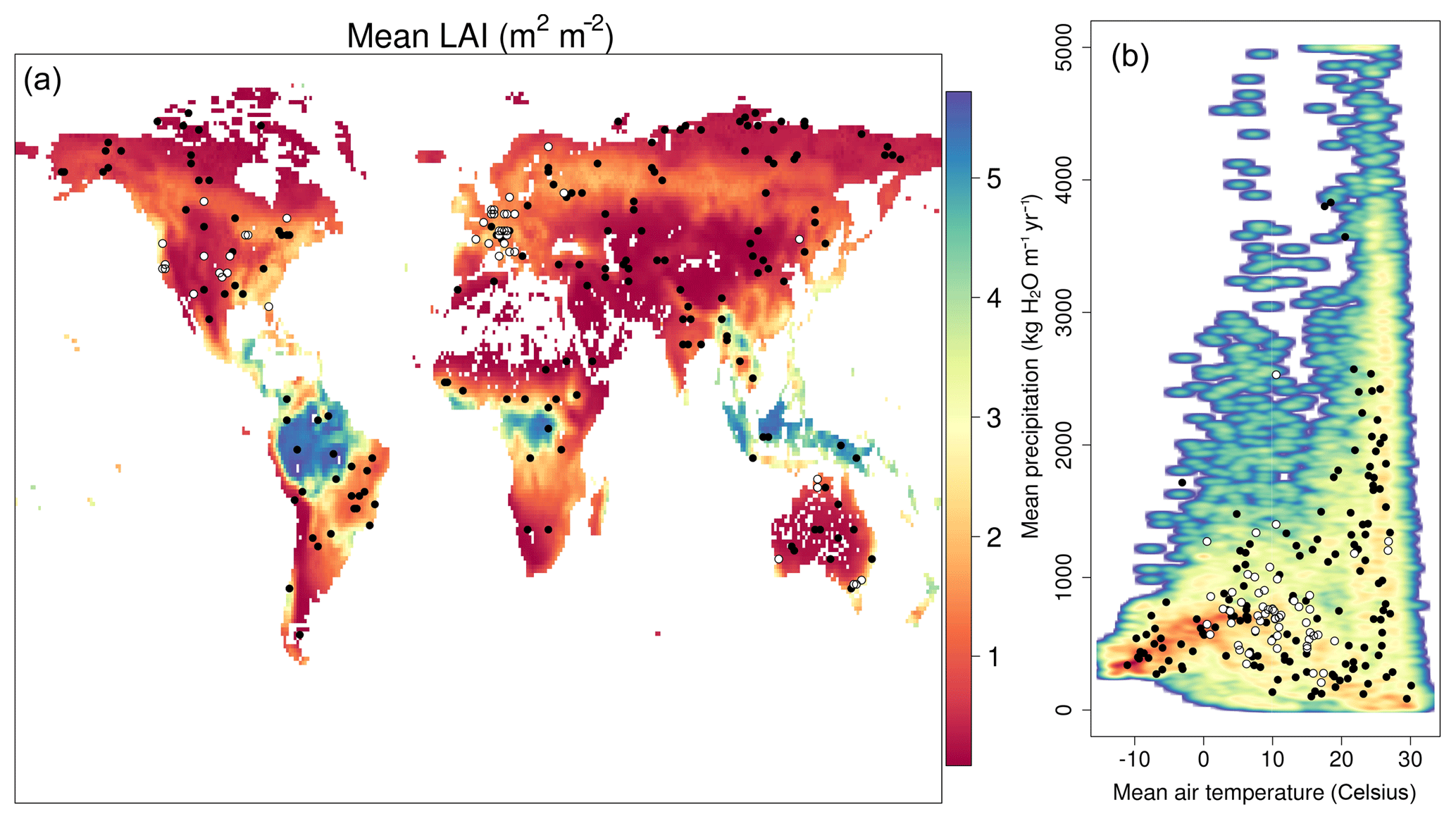
Figure 2(a) Global (1×1∘) mean LAI estimates (2001–2015) derived from NASA's MODIS product. (b) Climate space described by mean annual precipitation and temperature (ECMWF's ERA-Interim; Dee et al., 2011). Shading indicates the point density, with red areas indicating high density. In both plots black circles show the location of SPA calibration sites, while the white circles with black rings show the FLUXNET2015 sites used to provide independent validation.
For both the calibration and validation simulations, SPA (and ACM-GPP-ET) require inputs of meteorological drivers, foliar nitrogen, soil textural information and time series of LAI and root biomass. Prescribing LAI and root biomass, opposed to coupling ACM-GPP-ET to a C-cycle model, allows the isolation of photosynthetic driver sensitivity without complex C-cycle feedbacks. Meteorological drivers were taken from the ERA-Interim reanalysis (Dee et al., 2011); these drivers were downscaled to an hourly time step using a weather generator (https://github.com/GCEL/WeatherGenerator_v1, last access: 29 April 2019). Atmospheric CO2 concentration for each day was sampled from 300 to 450 ppm; the exaggerated CO2 range is to ensure that influence of increasing CO2 concentrations is contained within the calibration dataset. Note that prescribing LAI, root biomass and fixing soil moisture at field capacity prevents propagation of unexpected/undesired responses to strongly increasing atmospheric CO2 gradients; i.e. each day's GPP and ET are purely as a function of that day's conditions. Mean foliar nitrogen content was randomly sampled for each site (but held constant over time) from log10 normal distribution (mean = 1.89 g N m−2; Kattge et al., 2011). Soil sand and clay contents were extracted from the Harmonized World Soils Database (HWSD; Hiederer and Köchy, 2011); locations for which the sand and clay content fall outside the parameterised bounds for the Saxton soil hydrological model were also excluded (∼0.7 % of global land surface). Time series of LAI and root stocks used to drive SPA and ACM-GPP-ET were extracted from a global terrestrial carbon cycle model–data fusion analysis (Bloom et al., 2016). We used LAI and fine roots datasets from Bloom et al. (2016) derived from MODIS LAI products, remotely sensed above-ground biomass and ecological process knowledge (for details, see Bloom and Williams, 2015).
In order to quantify the ability of the analysis framework to retrieve accurate ecophysiological trait information (e.g. optimum temperature of photosynthesis), a single set of ecophysiological parameters is used to drive SPA. This nominal parameter set is a combination of the forest hydraulic parameters from Williams et al. (1996) and broad-leaf forest radiation reflectance parameters from Smallman et al. (2013).
The hourly SPA simulations were aggregated to daily time step and then sub-sampled at a 2-weekly interval to reduce temporal auto-correlation. Further filtering was applied to remove days with zero GPP (i.e. winter) and days for which SPA was unable to solve its energy balance closure to a cumulative absolute error, over sub-daily time steps, of less than 50 W m−2 summed across each 24 h period. Thus, after filtering, some 42 658 simulation days were available for calibration.
3.1 SPA
The Soil Plant Atmosphere (SPA; Williams et al., 1996; Smallman et al., 2013) model simulates a mechanistic representation of the terrestrial ecosystem, coupling plant carbon and water cycles through ecophysiological principles. SPA simulates up to 10 canopy layers simulating both the sunlit and shaded leaf area, each being independently connected to water supply from the soil. Water accessibility from 20 soil layers is determined as a function of root penetration within each soil layer. SPA estimates the surface exchanges of heat, water and CO2 within a mass- and energy-balanced framework. SPA has been extensively validated at range of spatial scales (leaf to landscape) and climate zones (tropical, temperate and Arctic) (Williams et al., 1998, 2001b; Fisher et al., 2006, 2007; Sus et al., 2010; Smallman et al., 2013, 2014; López-Blanco et al., 2018). A detailed description of SPA and its major developments can be found in Williams et al. (1996, 1998, 2001b, 2005), Sus et al. (2010) and Smallman et al. (2013); however a brief description follows below.
Leaf-level photosynthesis (Farquhar; Farquhar and von Caemmerer, 1982), transpiration (Penman-Monteith; Jones, 1992) and energy balance are coupled via a mechanistic model of stomatal conductance (Williams et al., 1996; Bonan et al., 2014). Stomatal opening is modulated to optimise photosynthetic uptake within constraints determined by (i) the intrinsic water use efficiency and (ii) the balance of atmospheric demand with available water supply from the soil. SPA makes use of a detailed multi-canopy layer radiative transfer scheme estimating the absorption and reflectance of both short- and long-wave radiation for the sunlit and shaded leaf area (Williams et al., 1998). Aerodynamic exchange coefficients for water, heat and CO2 are estimated accounting for above-, within- and under-canopy momentum decay, including stability corrections based on the Monin–Obukov stability theorem (Smallman et al., 2013).
3.2 CARDAMOM
The CARbon DAta MOdel fraMework (CARDAMOM; Bloom and Williams, 2015) is a model–data fusion (MDF) framework. CARDAMOM uses a Bayesian approach within a Metropolis Hastings–Markov Chain Monte Carlo (MH-MCMC) algorithm to retrieve parameters for a given model as a function of observational constraints. Parameter priors are specified with a uniform probability distribution truncated between minimum and maximum values (Table 1). CARDAMOM was used to calibrate ACM-GPP-ET based on GPP, transpiration, soil evaporation and evaporation of intercepted rainfall provided by SPA.
For the purpose of calculating the cost function used within the MDF approach, we assumed uncertainties consistent with those expected from eddy covariance. The uncertainty of both GPP and evaporative fluxes is assumed to be 15 %, representing random error estimates typically found for eddy covariance (Stoy et al., 2006; Mauder et al., 2013). The use of the SPA model with known input parameters allows for quantification of how accurately the equivalent retrieved parameters have been determined. Where there is a directly equivalent parameter between SPA and ACM-GPP-ET, the SPA values are provided in Table 1.
ACM-GPP-ET is validated over two phases using a range of evapotranspiration and GPP estimates from (1) out-of-sample SPA simulations and (2) fully independent eddy-covariance-derived estimates from the FLUXNET2015 database.
4.1 SPA validation
Phase (1) tests the ability of ACM-GPP-ET to simulate the soil moisture dynamics and resulting feedbacks on plant photosynthesis and evaporation estimated by the state-of-the-art SPA model. To achieve this we compare out-of-sample SPA-simulated estimates of GPP and evapotranspiration. SPA's soil moisture status was held constant at field capacity during calibration phase and substantially sub-sampled. Here SPA's soil moisture status was allowed to vary as a function of its inputs and outputs; these simulations were carried out at the same locations as those used for the calibration analysis but without any sub-sampling.
4.2 Independent validation: FLUXNET2015
Phase (2) quantifies ACM-GPP-ET's predictive skill using fully independent observations. Furthermore, we contrast ACM-GPP-ET's predictive capacity with that of SPA. This is achieved by both ACM-GPP-ET and SPA simulating carbon and water fluxes at FLUXNET2015 sites. The SPA simulations use the same nominal set of ecophysiological parameters used in generating the calibration dataset. ACM-GPP-ET uses the maximum likelihood parameter set retrieved during the calibration procedure. The parameter set used here broadly represents a forest ecosystem. Therefore, we hypothesise that both SPA and ACM-GPP-ET will perform best at forest sites and less well at sites with different hydraulic traits.
Daily estimates of GPP and ET derived from eddy covariance were extracted from the FLUXNET2015 database (http://fluxnet.fluxdata.org/, last access: 1 November 2016). The FLUXNET2015 database was filtered to include only sites which overlapped our simulation period (2001–2015) for a minimum of 3 years, to allow for inter-annual comparison and not more than 20 % missing data. ACM-GPP-ET is designed to emulate the C3 photosynthetic pathway; therefore sites which are listed to be dominated by vegetation which use the C4 or Crassulacean acid metabolism (CAM) pathways were removed. We also removed estimates which do not carry the highest-quality flags to avoid comparing our model against estimates generated using a statistical model of net exchange (i.e. we use only the non-gap-filled observations). Eddy covariance estimates for which energy balance non-closure is less than 85 % were also rejected. In total 497 site years encompassing 10 vegetation types across 59 sites were available for validation of GPP and ET. Meteorological drivers used to drive SPA and ACM-GPP-ET were extracted from the local site-level measurements. Missing data were gap filled, either assuming linear interpretation (for single missing hours) or extracted from bias-corrected temporally downscaled meteorological drivers as used in the calibration process. Finally, as with the earlier SPA simulations, LAI and root biomass for each site are extracted from Bloom et al. (2016).
We show that a single global calibration of ACM-GPP-ET can effectively reproduce the patterns of GPP and ET simulated by SPA. Importantly the predictions of WUE are consistent for both ACM-GPP-ET and SPA, so that the simplified model is able to capture the interactions between C and water cycling. We also describe an independent validation against FLUXNET data, across 59 sites.
5.1 SPA calibration and validation
A single global ACM-GPP-ET parameterisation simulates the calibration dataset with a high degree of skill when using the maximum-likelihood parameter sets retrieved from the calibration analysis (Fig. 3). The dynamics of soil evaporation is best simulated by ACM-GPP-ET followed by GPP and transpiration, each achieving R2≥0.91. Evaporation of canopy-intercepted precipitation achieved a lower R2 at 0.81. All fluxes are largely unbiased (GPP bias g C m−2 d−1 and evaporative fluxes magnitude ≤0.08 kg H2O m−2 d−1), with low root mean square error (RMSE; 0.97 g C m−2 d−1 and ≤0.39 kg H2O m−2 d−1). However, we note a tendency to underestimate peaks in transpiration found in the SPA simulation (Fig. 3). Evaporation of canopy-intercepted precipitation is least well simulated by each metric used here; however this is expected given the sensitivity of this flux to the timing and intensity of precipitation events and the canopy energy balance varying strongly at sub-daily timescales which are not accounted for here. Transpiration (Etrans; 61 %) dominates the overall ACM-GPP-ET-simulated evaporative budget, followed by evaporation of canopy-intercepted rainfall (Ewet; 34 %) and soil surface evaporation (Esoil; 5 %), broadly consistent with those simulated by SPA in the calibration dataset (67 %, 28 % and 5 % respectively). ACM-GPP-ET is 2200 times faster than SPA, where ACM-GPP-ET requires ∼0.000007 s d−1 and SPA 0.015 CPU seconds per simulated day. Overall, ACM-GPP-ET simulates the calibration dataset with substantial skill and a substantial reduction in computational requirements.
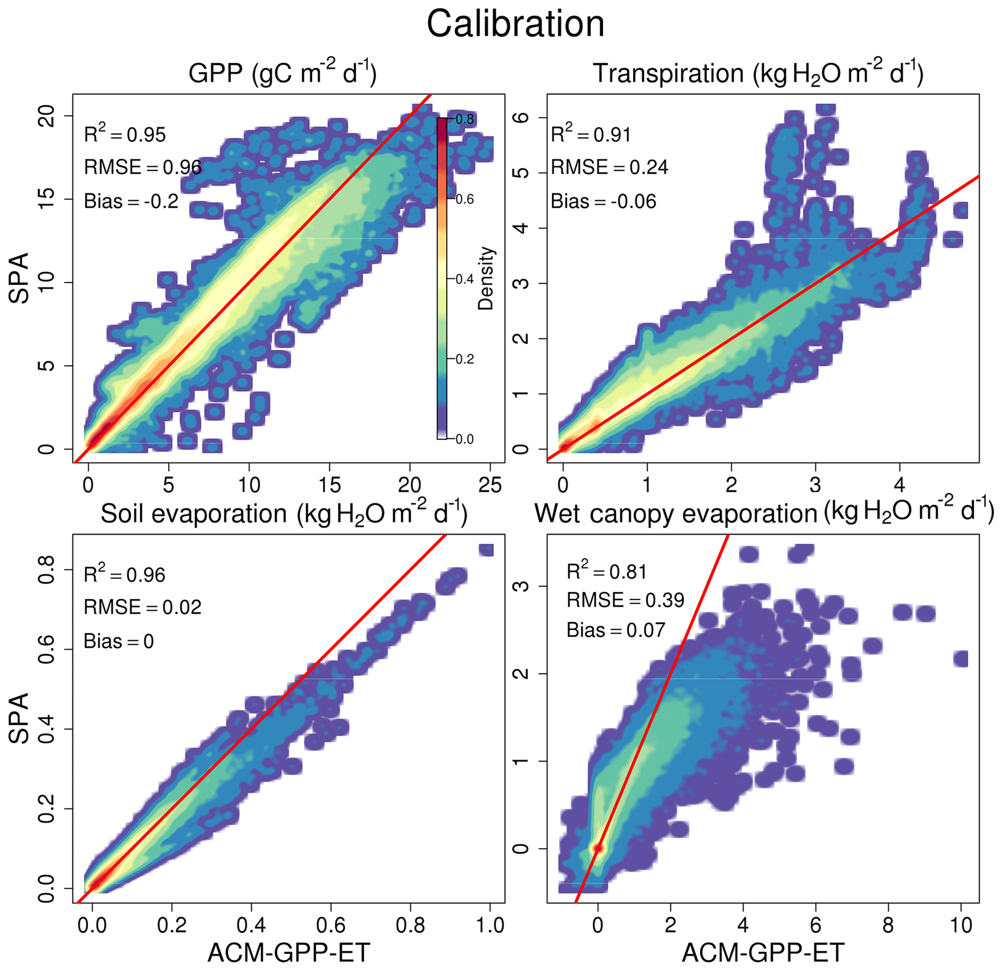
Figure 3Comparison between SPA- and ACM-GPP-ET-generated fluxes, where ACM-GPP-ET used the maximum likelihood parameter sets from the calibration procedure. Fluxes compared are gross primary productivity (g C m−2 d−1), transpiration (kg H2O m−2 d−1), soil evaporation (kg H2O m−2 d−1) and evaporation of water intercepted by the canopy (kg H2O m−2 d−1). The red line is a 1:1 line for reference. The colour intensity from blue to red indicates the density of flux estimates within a given area. Note that for clarity, to show low-density areas, the density values are scaled by density1∕4.
Simulation of carbon and water fluxes remains robust in the phase (1) validation where ACM-GPP-ET is compared against the out-of-sample SPA simulations in which soil moisture content is dynamically simulated, i.e. not held at field capacity as in the calibration procedure (Fig. 4). Similarly, partitioning between evaporative fluxes remains closely aligned between ACM-GPP-ET (Etrans=59 %, Ewet=35 %, Esoil=6 %) and SPA (Etrans=62 %, Ewet=31 %, Esoil=7 %). Only soil evaporation suffers a substantial reduction in the simulation of the variability of SPA's soil evaporation from R2=0.96 to 0.59 however remaining unbiased and the RMSE increasing by only 0.02 kg H2O m−2 d−1 (Fig. 4).
Ecosystem water use efficiency (WUE = GPP∕Etrans) simulated by SPA is well predicted by ACM-GPP-ET (R2=0.79, RMSE =1.88 g C per kg H2O, bias =0.33 g C per kg H2O). The consistency within simulations with dynamic water availability demonstrates resilience in ACM-GPP-ET's ability to represent the linkages between the plant carbon and water cycles, which is key when considering the impacts of climatic extremes such as the evolution of drought. This ability to simulate drought in a manor consistent with SPA is supported by the high-quality simulation of soil moisture content (R2=0.84, RMSE =4.19 kg H2O m−2, bias =1.17 kg H2O m−2; Fig. 4).
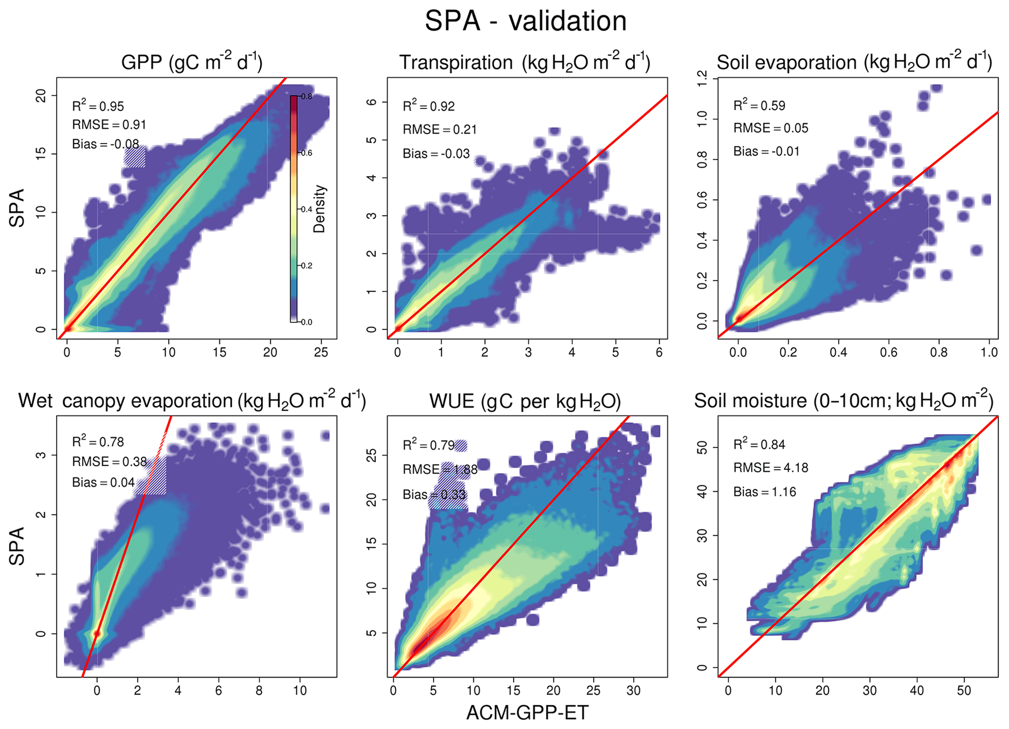
Figure 4Comparison between ACM-GPP-ET- and SPA-simulated fluxes for model-based validation of ACM-GPP-ET's ability to simulate coupled plant carbon and water cycle dynamics. ACM-GPP-ET uses the maximum likelihood parameter set from the calibration procedure. Fluxes compared are gross primary productivity (g C m−2 d−1), transpiration (kg H2O m−2 d−1), soil evaporation (kg H2O m−2 d−1) and evaporation of water intercepted by the canopy (kg H2O m−2 d−1). Also shown is the soil moisture content in the 0–10 cm soil layer (kg H2O m−2) and water use efficiency (WUE = GPP∕T; g C/kg H2O). The red line is a 1:1 line for reference. The colour intensity from blue to red indicates the density of flux estimates within a given area. Note that for clarity, to show low-density areas, the density values are scaled by density1∕4.
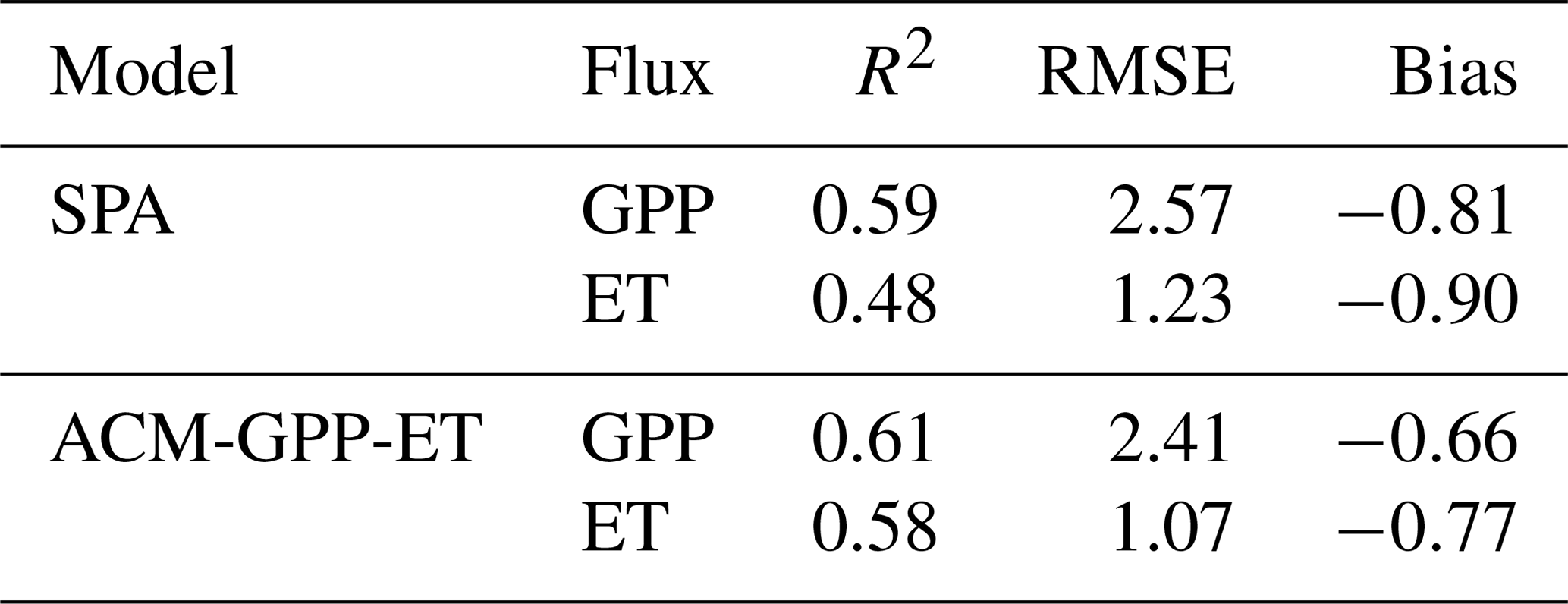
Table 4Summary statistics for the global comparison between GPP and ET estimated by both ACM-GPP-ET and SPA from the FLUXNET2015 database. Statistics include R2, root mean square error (RMSE) and mean bias (model−obs). GPP units are g C m−2 d−1, and ET is in units of kg H2O m−2 d−1.
5.2 FLUXNET2015: independent validation
For phase (2) validation, ACM-GPP-ET and SPA simulated GPP and ET estimates for 59 sites from the FLUXNET2015 database to provide fully independent validation of ACM-GPP-ET's ability to simulate real-world estimates but also of its predictive skill compared to that of SPA (Table 4; Fig. 5). For the FLUXNET validation we aim to achieve a similar degree of predictive capacity to existing remote-sensing-driven estimates. As stated earlier we hypothesise that both ACM-GPP-ET and SPA will perform better at forest sites than in other ecosystems. GPP is typically better predicted than ET by both ACM-GPP-ET and SPA, which is expected given that ET is the combination of three evaporative fluxes (ET ). Both GPP and ET are underestimated by ACM-GPP-ET and SPA, with larger RMSEs than found when comparing between ACM-GPP-ET and SPA simulations (Table 4). However, ACM-GPP-ET marginally outperforms SPA at most sites and for ET in particular. The between-site distribution of R2 and RMSE is skewed, with a relatively small number of sites performing poorly (Fig. 5). For each metric shown (R2, RMSE and bias) the distribution achieved by ACM-GPP-ET indicates a potentially greater degree of predictive skill at a daily time step than SPA.
ACM-GPP-ET and SPA perform well at forested sites (except evergreen broad-leaf forests), with more variable performance in grassland-, crop- and savannah-type ecosystems (Fig. 6). However, both ACM-GPP-ET and SPA demonstrated a clear capability to simulate inter-site variation (i.e. the mean GPP and/or ET between sites), with R2∼0.94 for both GPP and ET. Variation in predictive capability is not unexpected given that we use a single set of parameters for both models without site-specific modifications.
ACM-GPP-ET-simulated and eddy-covariance-derived estimates of GPP and ET were compared at different temporal aggregations (weekly, monthly and annual), showing good skill at simulating seasonal and inter-annual dynamics. From daily through to weekly and monthly aggregation, the statistical agreement between variation in simulated and observed estimates improves considerably. Estimation of ET is most improved, increasing from R2=0.58 to 0.72 to 0.75, while for GPP R2 increases from 0.61 to 0.65 to 0.68. RMSE and mean bias remain largely unchanged. However, simulation of inter-annual variation is more challenging with the R2 for GPP =0.68 and ET =0.46. A similar pattern of results is found for SPA (not shown).
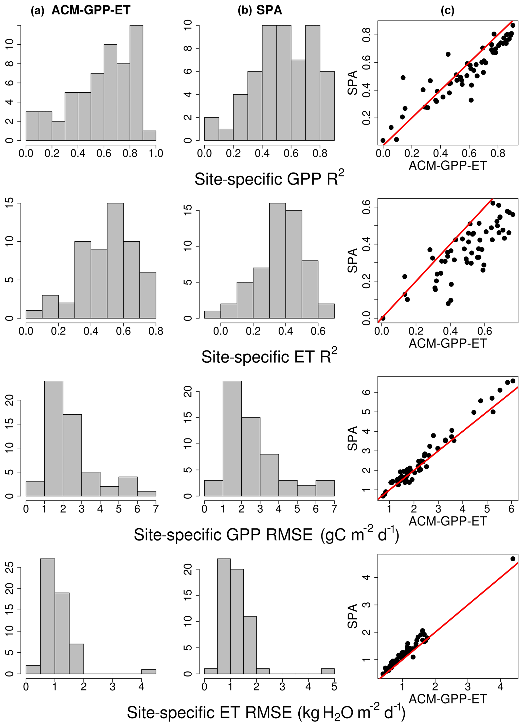
Figure 5Comparison of ACM-GPP-ET and SPA simulating fully independent gross primary productivity (GPP) and evapotranspiration (ET) from FLUXNET2015. The histograms show the site-specific R2 and RMSE. SPA is shown in (a), and ACM-GPP-ET is in (b). The panels in (c) show the site-by-site comparison of statistical metrics achieved by each model.
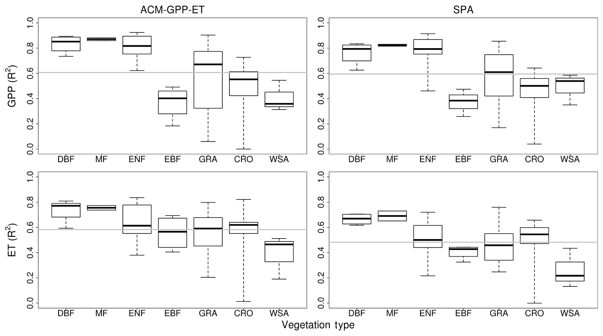
Figure 6Independent validation of ACM-GPP-ET and SPA using eddy-covariance-derived estimates of gross primary productivity (GPP) and evapotranspiration (ET) from the FLUXNET2015 database. Box and whisker plots show the site-specific R2 values for each of the International Geosphere-Biosphere Programme (IGBP) vegetation classification. CRO is cropland, CSH is closed canopy shrubland, DBF is deciduous broad-leaf forest, EBF is evergreen broad-leaf forest, ENF is evergreen needle-leaf, GRA is grassland, MF is mixed forest and WSA is woody savanna. The mean for each vegetation classification is shown by the thick centre line, and the box represents the 25 % and 75 % quantiles, while the whiskers indicate the minimum and maximum values. The horizontal grey line indicates the mean R2 across groups.
In this study we have described, calibrated (Fig. 3) and validated (Figs. 4–7) a model of intermediate complexity, the aggregated canopy model for gross primary productivity and evapotranspiration (ACM-GPP-ET v1). ACM-GPP-ET provides a process-orientated representation of plant photosynthesis and the water cycle, coupled through ecophysiological principles (Fig. 1). ACM-GPP-ET simulations using a single global calibration have been validated against simulated GPP and evaporative fluxes but also emergent properties including WUE and soil moisture status from the state-of-the-art SPA model. These simulations were driven with LAI, fine root stock and meteorological conditions spanning across global gradients (Fig. 2). Furthermore, to provide fully independent validation we have compared our estimated GPP and ET fluxes, again using a single global calibration, against multiple eddy-covariance-derived flux data from the FLUXNET2015 database, demonstrating substantial predictive skill.
6.1 ACM-GPP-ET: lessons learned on model simplification
A number of alternative model structures were tested over the course of the development of ACM-GPP-ET, and while it is beyond the scope of this study to describe these in detail, there are a range of important lessons learned from the development of specific components. The single most computationally expensive component is the iterative solution linking photosynthesis and transpiration via stomatal conductance. However, a coupled representation of stomatal conductance linking these processes was essential for maintaining the predictive capacity of both canopy exchanges and emergent properties of WUE and soil moisture status. Similarly, the simulation of soil moisture dynamics is time-consuming, due to the need for simulating non-linear drainage processes occurring at sub-daily time steps. Originally a single-layer bucket was tested but was unable to generate reasonable soil moisture dynamics and ultimately drought responses compared with SPA. Our experience is consistent with other studies which have explicitly considered the impact of varying the number of soil moisture layers (Blyth and Daamen, 1997). Water drainage between soil layers and run-off of water from the canopy surface places an upper limit on efficiency achievable while maintaining predictive skill for soil moisture status and, indirectly, canopy fluxes. However, we expect further efficiency improvements to be achievable through subsequent code modifications including alternative theoretical approaches to achieve the photosynthesis–transpiration coupling. A dedicated focus on code optimality is beyond the scope of the current study but is critical to the ongoing process of model improvement.
In this study 22 parameters are calibrated (Table 3); 15 of these are related to the estimation of canopy and/or soil absorption of PAR, NIR and long-wave radiation. The key challenge for the radiative transfer was the essential requirement to reproduce the emergent non-linear functional shape between LAI and canopy radiation absorption, transmittance to soil and reflectance, making the complex vertical structure implicit in the calibration. We found an appropriate simulation of non-linear radiative transfer was critical for realistic radiative responses of each component of evaporation. In contrast, for a GPP model alone, a far simpler radiative transfer scheme was viable (Williams et al., 1997). However, the large number of parameters in the radiative transfer scheme is open to constraint through, for example, remote sensing observations of canopy structure and reflectance. These observations could be used to calibrate the scheme for individual locations but also canopy structural forms (i.e. canopy vertical structure).
6.2 Intermediate complexity emulation of a complex TEM
ACM-GPP-ET accurately simulates its calibration dataset (Fig. 3) and out-of-sample validation (Fig. 4) generated by the SPA model. Substantial predictive skill was achieved for photosynthesis and each of the evaporative fluxes but also the unbiased simulation of soil moisture and WUE, which were not part of the calibration process (Fig. 4). The single global calibration effectively spans global process sensitivity to climate across gradients of latitude, maritime–continental gradients and seasonal cycles. The calibration also represents the effect of ecological variation of LAI and fine root stocks. By including 10 different drivers, we generated a major challenge for model simplification. ACM-GPP-ET must robustly represent functional forms for C and water cycling across these multiple response dimensions, including any interactions. We note an underestimate in peak transpiration fluxes (Fig. 3) which we hypothesise is due to the lack of including the impact of energy balance in canopy and non-linear responses at sub-daily timescales. While this bias may in some cases lead to an underestimate of within-day drought/water supply limitation, the statistical analyses for validation indicate that the functional forms embedded in ACM-GPP-ET effectively represent those arising from complex mechanistic interactions within SPA. ACM-GPP-ET generates robust daily aggregations from SPA's hourly resolution. ACM-GPP-ET effectively reproduces the ecoclimatological sensitivity of plant water use efficiency from the SPA model (Fig. 4). Reliable simulation of the dynamics and magnitude of plant WUE is an important property for robust modelling of hydrological, ecological and biological interactions. For climate sensitivity studies, ecosystem carbon–water coupling controls drought development and its interactions with ecosystem processes (Beer et al., 2009; Keenan et al., 2013; Bonan et al., 2014). Similarly, appropriate partitioning of evaporative fluxes, i.e. T∕ET, is essential to simulate the overall ecosystem response to change in climate correctly. Transpiration has a direct interaction with biogeochemical cycling through canopy conductance, whereas evaporative fluxes have an indirect effect through adjustments to soil moisture and radiation environment mediated through variation in canopy cover. T∕ET estimated by ACM-GPP-ET and SPA is closely aligned for both the calibration procedure with fixed soil moisture and that with dynamic soil moisture. The fraction of T∕ET declined under dynamic soil moisture in both models, indicating a consistent response to varied water status. This consistency indicates that ACM-GPP-ET effectively represents and aggregates the critical nexus for carbon and water cycling simulated in the leaf-scale stomatal conductance routines of SPA to canopy scale. As noted in Sect. 6.1 alternative coupling approaches could be investigated to reduce the computational requirements, but perhaps more importantly our framework allows for the testing of alternative coupling hypotheses to robustly assess their predictive capacity against emergent properties. For example, recent analyses estimate that transpiration is responsible for ∼58 % of global evaporation, consistent with both SPA and ACM-GPP-ET estimates and contrasting with many TEMs which tend to underestimate T∕ET partitioning (Wei et al., 2017) but also expanding on the stomatal model comparison conducted by Bonan et al. (2014).
6.3 Comparison to independent flux observations worldwide
A key component of our validation process was the comparison of ACM-GPP-ET- and SPA-simulated GPP and ET fluxes at 59 FLUXNET2015 sites. We aimed to achieve a comparable predictive skill compared to analyses driven by remotely sensed information. Moreover, we hypothesised that both ACM-GPP-ET and SPA would perform best at forest sites due to the choice of forest-based parameters used in the calibration procedure. ACM-GPP-ET and SPA simulated both GPP and ET fluxes with substantial skill, especially given that only a single global parameterisation was used (Table 4; Figs. 5–6). Indeed, ACM-GPP-ET slightly outperforms SPA in each statistical metric presented here; the greatest difference is found for simulating daily variation of GPP and in particular ET fluxes (Fig. 5). However, it is unlikely that ACM-GPP-ET has actually improved on SPA itself, as ACM-GPP-ET is an emulation of SPA; therefore the difference should not be viewed as significant. The improved statistics found for ACM-GPP-ET are likely due to a combination of factors underlying errors which by chance lead to an apparent improvement. One exception to this assumption is that SPA's sub-daily meteorological drivers were gap filled based on downscaled reanalysis drivers (as used in the calibration process), which, as noted in the Introduction, can introduce errors comparable in magnitude to the direct daily aggregation (e.g. Williams et al., 2001a). Finally, as hypothesised SPA and ACM-GPP-ET performed best at forests sites, with some grassland, cropland and woody savanna sites performing less well (Fig. 6). The relative pattern of performance between vegetation types is consistent between ACM-GPP-ET and SPA, strongly indicating a consistent underlying response to a wide range of climate conditions and ecological states and similar predictive capabilities when applied in circumstances without site-specific information.
The ACM-GPP-ET predictions used a single, global calibration and thus evaluated a single response surface to FLUXNET data, without taking into account any ecological variation in plant processes among FLUXNET sites beyond LAI, fine root biomass and soil textural information (potential errors in these components are discussed below). Thus, critical plant traits, such as the maximum rate of carboxylation per leaf area (Vcmax), stem hydraulic conductance (Gp) and rooting depth, were set the same across all sites for SPA and ACM-GPP-ET. But, we expect these parameters to vary, given our knowledge of trait variation at sites and from worldwide studies (Wright et al., 2004; Kattge et al., 2011; Johnson et al., 2018). So, the global parameterisation is likely to be biased for most sites. The poorer performance of SPA and ACM-GPP-ET in predicting GPP in evergreen deciduous forests is likely linked to a bias in parameters, for example (Fig. 5). For a more robust global application, ACM-GPP-ET requires prior estimates for local values of the parameters in Table 3. Based on previous works by Bonan et al. (e.g. 2014), we expect the most important local parameterisation will be for root resistivity, plant conductivity and NUE. Root resistivity and plant conductance determine the maximum rates of water transport to the canopy. NUE determines the capacity of carboxylation and electron transport in photosynthesis.
Errors in the LAI, fine root biomass and soil textural information used in the SPA and ACM-GPP-ET model inputs are also likely. Errors in the remote sensing of LAI assimilated within the CARDAMOM framework will propagate into the resulting estimates of LAI and fine root biomass. Soil textural information comes from the HWSD, the errors for which are poorly described. Furthermore, we made assumptions about root depth and canopy height which are also likely biased. LAI information ultimately comes from MODIS (or other satellite products), which has varied skill depending on vegetation cover type (Yan et al., 2016). Yan et al. (2016) showed MODIS LAI detects LAI dynamics least well over forests (particularly needle-leaf), but perhaps more critically for our analysis they also showed a consistent RMSE between 0.6 and 0.8 m2 m−2 between vegetation types. For arable crop land and grassland, such an RMSE could constitute an error in the magnitude of LAI on the order of 66 % (in their observation dataset), potentially resulting in substantial errors and bias in estimation of ecosystem fluxes.
6.4 Comparison to other global GPP and ET estimates
We aimed for and achieved ACM-GPP-ET's performance against FLUXNET2015 sites to be comparable to that demonstrated by GPP and ET estimates generated by a range of alternative approaches and temporal resolutions (e.g. Jung et al., 2011; Mu et al., 2011; Martens et al., 2017; Wang et al., 2017). For example, FLUXCOM uses a machine-learning approach assimilation and a wide range of global spanning information to estimate monthly GPP (number of sites not reported: , RMSE g C m−2 d−1) and ET (number of sites not reported: , RMSE kg H2O m−2 d−1) (Jung et al., 2011). At monthly timescales FLUXCOM performs marginally better in the estimation of variation in fluxes but with RMSEs roughly half that found with ACM-GPP-ET for both GPP and ET; this is not unexpected as FLUXCOM was calibrated against the FLUXNET database itself (Jung et al., 2011), whereas the satellite-based remotely sensed derived 8 d MODIS estimates, based on absorbed radiation and empirical response functions, perform less favourably than ACM-GPP-ET for both GPP (18 sites, R2=0.52, RMSE =0.96 g C m−2 d−1; Wang et al., 2017) and ET (46 sites, R2=0.65, RMSE =0.84 kg H2O m−2 d−1; Mu et al., 2011). Finally, the Global Land Evaporation Amsterdam Model (GLEAM) estimates of ET performed similarly to those achieved by ACM-GPP-ET; GLEAM makes use of a comparatively complex approach to estimate ET, using a model of ecosystem water cycling updated by satellite-based remotely sensed information within a data assimilation framework to generate a daily estimate of the global water budget (63 sites, R2=0.64, RMSE =0.73 kg H2O m−2 d−1; Martens et al., 2017). In each case the approaches highlighted above made use of vegetation-type-specific information or location-specific remotely sensed biophysical information to drive their analysis compared to our comparatively naive approach using a single set of ecophysiological parameters. Therefore, we reasonably expect significant improvements through the inclusion of location- and/or vegetation-type-specific calibration as would be achieved through model–data fusion approaches (e.g. Bloom et al., 2016). A key benefit of our process-orientated approach is that unlike the above-described approaches, which are each dependent on the input of remotely sensed information, our modelling framework can be used predictively to extrapolate into space and times for which remotely sensed information are not available. This is particularly true when ACM-GPP-ET has been coupled to our DALEC C-cycle model, allowing for feedbacks between carbon supply and available LAI. Further details on the potential of this coupling are below.
6.5 Global applications
It is typical to generate regional and global estimates of carbon and water cycling using complex land surface models. Such models make vital contributions to assessments of the global carbon budget (Le Quéré et al., 2015) and weather and climate forecasts. A challenge for these models is that their complexity generates high computational demand, and they have demanding parameterisation needs. Thus, these models are often applied using plant-functional-type approaches, whereby parameters are set for an entire biome, with no variation, and no uncertainty is attached. There is a need then for models of intermediate complexity that are less demanding computationally and have fewer parameters but retain realism.
ACM-GPP-ET is such a model, constructed from the simplification of a complex land surface model with a long evaluation history, SPA. ACM-GPP-ET captures the critical functional forms in carbon–water interactions that emerge from process representation at sub-canopy, hourly timescales. ACM-GPP-ET can represent the interactions of supply and demand on stomatal opening and how this responds to changes in atmospheric conditions and soil moisture states. This level of detail is critical for application in global change analyses that are vital for diagnosing and predicting earth system evolution. Thus, ACM-GPP-ET produces realistic outputs, based on comparison with its more complex precursor.
ACM-GPP-ET is well suited for ensemble modelling schemes due to its faster runtime, as shown in the MH-MCMC calibration process used here with SPA outputs used as training data. The parameter posteriors generated here (Fig. A1) provide a starting point for full carbon cycle and water cycle analyses across regional to global domains. For instance, Bloom et al. (2016) have shown how an IC GPP model, ACM-GPP (Williams et al., 1997), combined with a carbon cycling model (DALEC; Williams et al., 2005), can be linked into a model–data fusion framework, CARDAMOM. CARDAMOM can, when combined with DALEC, retrieve probabilistic estimates of carbon stocks, fluxes and model parameters (including key unknowns such as photosynthate allocation to plant tissues and their residence times). CARDAMOM can produce outputs across a domain at the resolution of input forcing (climate data, burned area) and observational constraints (satellite time series of LAI, biomass maps, soil C maps). The advantage of CARDAMOM is that it generates likelihoods for model initial conditions and parameter values that are consistent with climate forcing and domain observations from, for example, satellites, and their estimated errors. Currently CARDAMOM infers water limitations to C cycling through satellite observations of greenness alone. Because there is no coupling to a local water model, CARDAMOM cannot use modelled information on water balance or independent observations such as surface soil moisture (e.g. Chen et al., 2018). Through using ACM-GPP-ET in CARDAMOM, it will be possible to assimilate new observational data related to water fluxes and state variables.
The combination of ACM-GPP-ET, coupled to DALEC, and CARDAMOM provides multiple direct and indirect avenues for propagating information acquired using intermediate complexity models to complex state-of-the-art TEMs. ACM-GPP-ET and SPA directly share five parameters calibrated in this study (Table 2) plus a further nine biophysical traits which were not calibrated in this study (Table 3). Moreover, all of the parameters calibrated in this study (Table 2) can be indirectly related to those used in SPA (and many other TEMs), e.g. NUE, which is closely related to Vcmax, Jmax and foliar nitrogen but also radiation absorption and reflectance as a function of LAI. Similarly, when ACM-GPP-ET is combined with DALEC and used within the CARDAMOM framework, analyses such as those carried out by Bloom et al. (2016) (as is intended) retrieving information on carbon stocks, carbon allocation and residence times result in the retrieval of ecologically relevant traits. These traits can be directly related to parameters found in most state-of-the-art TEMs equipped with a C cycle. Such information should at a minimum provide information on spatial variation expected and in the optimum situation inform the researcher of the exact magnitude of those parameters.
6.6 Further opportunities and gaps
There are an array of next steps to undertake for further development both as a stand-alone tool and as part of a coupled modelling framework along with DALEC and CARDAMOM. The ACM-GPP-ET parameters estimated here against SPA can be calibrated individually at the FLUXNET2015 site (where sufficient biophysical information is available) to determine critical parameter variability to explain observed differences in fluxes. Driven with remotely sensed LAI, ACM-GPP-ET could make global estimates of GPP, ET and WUE for direct comparison with outputs from FLUXCOM, GLEAM and CMIP5 model ensembles. As part of the CARDAMOM framework, a site-specific FLUXNET2015 analysis allows us to assess our ability to retrieve information on the whole carbon cycle across ecological and climate gradients within a data-rich environment, including key unknowns such as rooting depths, which play a critical role in ecosystem resilience to drought. Such analyses provide the supporting frameworks needed to conduct global-scale reanalyses and potentially near-term (next 12 months) and intermediate-term (next 10 years) predictions with fully resolved uncertainties due to the propagation of ensembles.
Due to lack of space we have not reviewed the uncertainty estimates on parameter retrievals in the calibration of ACM-GPP-ET from SPA, but these contain useful information on the relative uncertainties in key processes in the aggregation. There are gaps in the capacity of ACM-GPP-ET globally; C4 pathways have not been included, nor organic soils. However, SPA is capable of simulating flux responses to these process adjustments, so new calibrations and/or model structure can be generated following a similar approach to that laid out here.
We have calibrated and robustly validated a model of intermediate complexity, ACM-GPP-ET, demonstrating good capacity for simulating the carbon–water dynamics of a state-of-the-art SPA model. ACM-GPP-ET has demonstrated substantial predictive skill when simulating fully independent eddy-covariance-derived estimates of carbon and water exchange, which is comparable to that of other globally used GPP and ET products. Finally, ACM-GPP-ET is highly computationally efficient, ∼2200 times faster than SPA, opening up a substantial range of further opportunities.
The code for ACM-GPP-ET version 1 has been made freely available from Edinburgh DataShare (doi: https://doi.org/10.7488/ds/2480; Smallman and Williams, 2018). Subsequent source code developments will be made available under GNU General Public License (GPL) via GitHub (https://github.com/GCEL/ACM_GPP_ET/releases, last access: 29 April 2019). The Fortran source code for the Weather Generator v1 used when downscaling daily meteorology to hourly time step is available at https://github.com/GCEL/WeatherGenerator_v1 (Smallman and Williams, 2019).
The CARDAMOM calibration process of ACM-GPP-ET retrieves multiple parameter sets consistent with the calibration dataset, resulting in a probability density function (PDF) for each parameter. A detailed discussion of the PDFs retrieved is beyond the scope of this study; however a brief description of the primary features is given below (Fig. A1).
The width (relative to the prior range) and overall shape of the PDF (i.e. uni- or multi-modal) give an indication of the constraint achieved. The majority of parameter posteriors (16 out of 22) cover less than 50 % of their prior range and show a single clear peak value without substantial skew (e.g. NUE; Fig. A1). Notable exceptions include aPAR_trans and kPAR_refl, indicating that there is a degree of equifinality in the absorption of PAR required to support photosynthesis and canopy evaporation. Therefore, this provides a potential focus for refinement of the model or calibration process (e.g. through the introduction of new data streams).
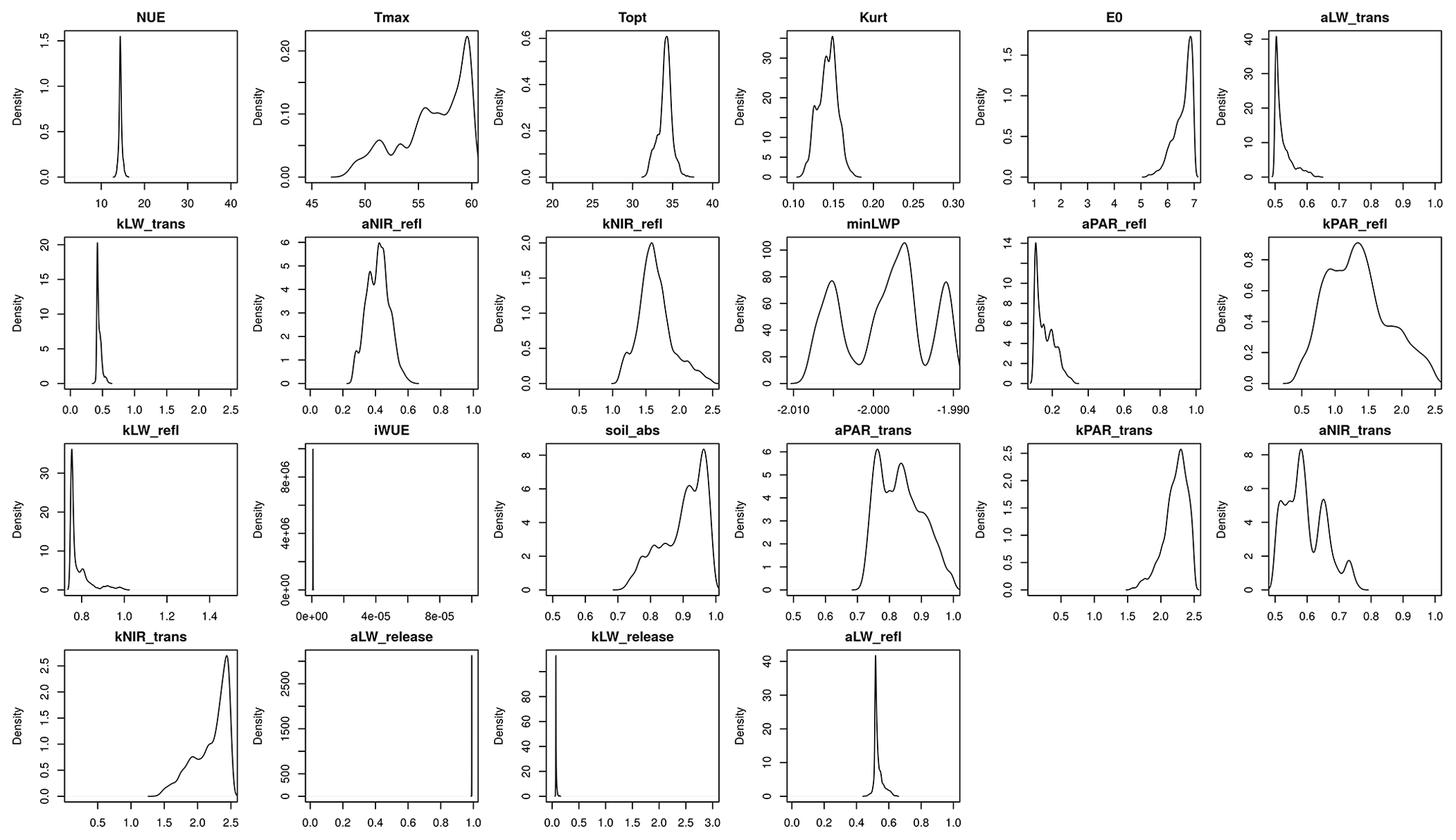
Figure A1Probability density functions of the retrieved parameters for ACM-GPP-ET. The figure label refers to the name given in Table 2 of the main text. The range of the x axis matches that of the parameter prior ranges to allow easy identification of those parameters which are the easiest to constrain.
Table B1Ecophysiological parameters used by SPA within this study but not already provided in Tables 2 and 3. These parameters are drawn from previous SPA publications (Williams et al., 1996; Bonan et al., 2014).
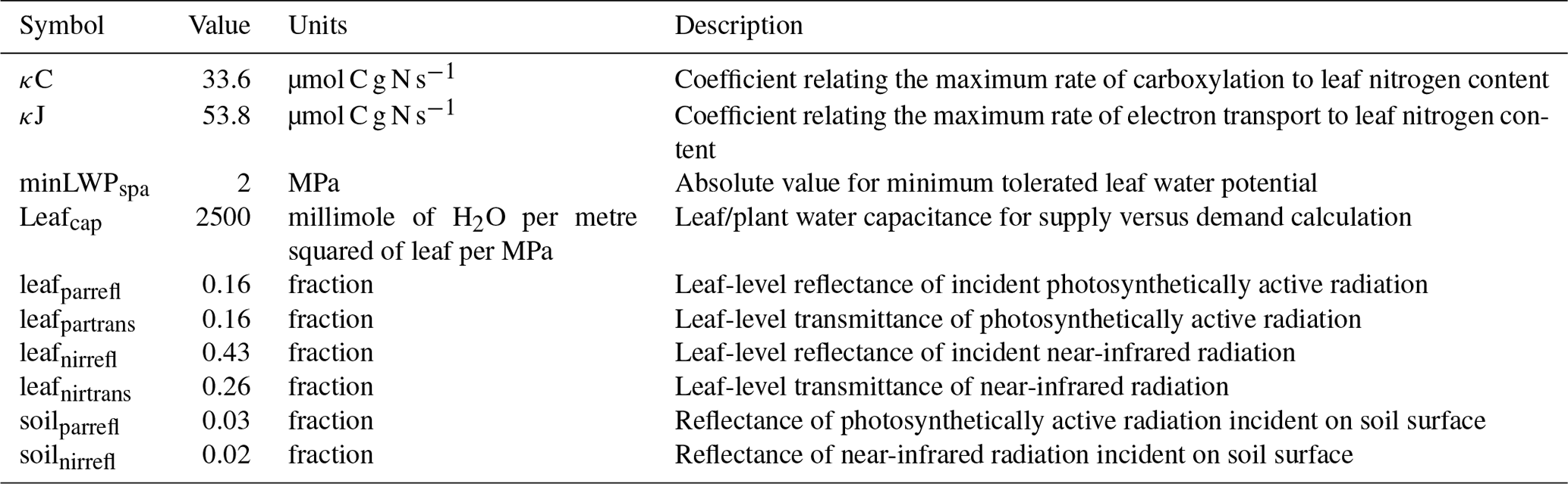
TLS coded the model and conducted the analysis. Both TLS and MW developed the experimental design and wrote the paper.
The authors declare that they have no conflict of interest.
This work used eddy covariance data (FLUXNET2015) acquired and shared by the FLUXNET community, including these networks: AmeriFlux, AfriFlux, AsiaFlux, CarboAfrica, CarboEuropeIP, CarboItaly, CarboMont, ChinaFlux, Fluxnet-Canada, GreenGrass, ICOS, KoFlux, LBA, NECC, OzFlux-TERN, TCOS-Siberia and USCCC. The ERA-Interim reanalysis data are provided by ECMWF and processed by LSCE. The FLUXNET eddy covariance data processing and harmonisation were carried out by the European Fluxes Database Cluster, AmeriFlux Management Project and Fluxdata project of FLUXNET, with the support of CDIAC and ICOS Ecosystem Thematic Center and the OzFlux, ChinaFlux and AsiaFlux offices. The study has been supported by the TRY initiative on plant traits (http://www.try-db.org, last access: 9 December 2015). The TRY initiative and database are hosted, developed and maintained by Jen Kattge and Gerhard Bönisch (Max Planck Institute for Biogeochemistry, Jena, Germany). TRY is currently supported by DIVERSITAS/Future Earth and the German Centre for Integrative Biodiversity Research (iDiv) Halle-Jena-Leipzig. This work was funded primarily through the NERC GHG program GREENHOUSE project (grant NE/K002619/1) and the UK Space Agency Forests2020 project (https://ecometrica.com/space/forests2020, last access: 3 June 2019). Additional resources were provided by the NERC National Centre for Earth Observations (NCEO).
This research has been supported by the Natural Environment Research Council (grant no. NE/K002619/1) and the UK Space Agency (grant no. Forests2020, as part of the International Partnerships Programme (IPP)).
This paper was edited by Christoph Müller and reviewed by Martin De Kauwe and one anonymous referee.
Beers, C., Ciais, P., Reichstein, M., Baldocchi, D., Law, B. E., Papale, D, Soussana, J. F., Ammann, C., Buchmann, N., Frank, D., Gianelle, D., Janssens, I. A, Knohl, A., Koestner, B., Moors, E., Roupsard, O., Verbeeck, H., Vesala, T., Williams, C. A., and Wohlfahrt, G.: Temporal and among-site variability of inherent water use efficiency at the ecosystem level, Global Biogeochem. Cy., 23, GB2018, https://doi.org/10.1029/2008GB003233, 2009. a, b
Bloom, A. A. and Williams, M.: Constraining ecosystem carbon dynamics in a data-limited world: integrating ecological “common sense” in a model–data fusion framework, Biogeosciences, 12, 1299–1315, https://doi.org/10.5194/bg-12-1299-2015, 2015. a, b, c, d, e
Bloom, A. A., Exbrayat, J.-F., van der Velde, I. R., Feng, L., and Williams, M.: The decadal state of the terrestrial carbon cycle: Global retrievals of terrestrial carbon allocation, pools, and residence times, P. Natl. Acad. Sci. USA, 113, 1285–1290, https://doi.org/10.1073/pnas.1515160113, 2016. a, b, c, d, e, f, g, h
Blyth, E. M. and Daamen, C. C.: The accuracy of simple soil water models in climate forecasting, Hydrol. Earth Syst. Sci., 1, 241–248, https://doi.org/10.5194/hess-1-241-1997, 1997. a
Bonan, G. B. and Doney, S. C.: Climate, ecosystems, and planetary futures: The challenge to predict life in Earth system models, Science, 359, 6375, https://doi.org/10.1126/science.aam8328, 2008. a, b, c
Bonan, G. B., Williams, M., Fisher, R. A., and Oleson, K. W.: Modeling stomatal conductance in the earth system: linking leaf water-use efficiency and water transport along the soil–plant–atmosphere continuum, Geosci. Model Dev., 7, 2193–2222, https://doi.org/10.5194/gmd-7-2193-2014, 2014. a, b, c, d, e, f, g, h, i, j, k, l, m, n, o
Bonan, G. B., Patton, E. G., Harman, I. N., Oleson, K. W., Finnigan, J. J., Lu, Y., and Burakowski, E. A.: Modeling canopy-induced turbulence in the Earth system: a unified parameterization of turbulent exchange within plant canopies and the roughness sublayer (CLM-ml v0), Geosci. Model Dev., 11, 1467–1496, https://doi.org/10.5194/gmd-11-1467-2018, 2018. a
Buckley, T. N., Cescatti, A., and Farquhar, G. D.: What does optimization theory actually predict about crown profiles of photosynthetic capacity when models incorporate greater realism?, Plant Cell Environ., 36, 1547–1563, https://doi.org/10.1111/pce.12091, 2013. a
Chen, F., Crow, W. T., Bindlish, R., Colliander, A., Burgin, M. S., Asanuma, J., and Aida, K.: Global-scale evaluation of SMAP, SMOIS, ASCAT soil moisture products, Remote Sens. Environ., 214, 1–13, https://doi.org/10.1016/j.rse.2018.05.008, 2018. a
Coble, A. P., VanderWall, B., Mau, A., and Cavaleri, M. A.: How vertical patterns in leaf traits shift seasonally and the implications for modelling canopy photosynthesis in a temperate deciduous forest, Tree Physiol., 36, 1077–1091, https://doi.org/https://doi.org/10.1093/treephys/tpw043, 2016. a
Collatz, G., Ball, J., Grivet, C., and Berry, J.: Physiological and environmental-regulation of stomatal conductance, photosynthesis and transpiration – a model that includes laminar boundary-layer, Agr. Forest Meteorol., 54, 107–136, https://doi.org/10.1016/0168-1923(91)90002-8, 1991. a
Dee, D. P., Uppala, S. M., Simmons, A. J., Berrisford, P., Poli, P., Kobayashi, S., Andrae, U., Balmaseda, M. A., Balsamo, G., Bauer, P., Bechtold, P., Beljaars, A. C. M., van de Berg, L., Bidlot, J., Bormann, N., Delsol, C., Dragani, R., Fuentes, M., Geer, A. J., Haimberger, L., Healy, S. B., Hersbach, H., Hólm, E. V., Isaksen, L., Kållberg, P., Köhler, M., Matricardi, M., McNally, A. P., Monge-Sanz, B. M., Morcrette, J.-J., Park, B.-K., Peubey, C., de Rosnay, P., Tavolato, C., Thépaut, J.-N., and Vitart, F.: The ERA-Interim reanalysis: configuration and performance of the data assimilation system, Q. J. Roy. Meteor. Soc., 137, 553–597, https://doi.org/10.1002/qj.828, 2011. a, b, c
Fan, Y., Miguez-Macho, G., Jobbágy, E. G., Jackson, R. B., and Otero-Casal, C.: Hydrologic regulation of plant rooting depth, P. Natl. Acad. Sci. USA, 114, 10572–10577, https://doi.org/10.1073/pnas.1712381114, 2017. a
Farquhar, G. D. and von Caemmerer, S.: Modelling of photosynthetic response to the environment, in: Physiological Plant Ecology II, Encyclopedia of Plant Physiology, Springer-Verlag, Berlin, 1982. a, b
Fer, I., Kelly, R., Moorcroft, P. R., Richardson, A. D., Cowdery, E. M., and Dietze, M. C.: Linking big models to big data: efficient ecosystem model calibration through Bayesian model emulation, Biogeosciences, 15, 5801–5830, https://doi.org/10.5194/bg-15-5801-2018, 2018. a
Fisher, R. A., Williams, M., Do Vale, R. L., Da Costa, A. L., and Meir, P.: Evidence from Amazonian forests is consistent with isohydric control of leaf water potential, Plant Cell Environ., 29, 151–165, https://doi.org/10.1111/j.1365-3040.2005.01407.x, 2006. a
Fisher, R. A., Williams, M., Da Costa, A. L., Malhi, Y., Da Costa, R. F., Almeida, S. and Meir, P.: The response of an Eastern Amazonian rain forest to drought stress: results and modelling analyses from a throughfall exclusion experiment, Glob. Change Biol., 13, 2361–2378, https://doi.org/10.1111/j.1365-2486.2007.01417.x, 2007. a
Fisher, R. A., Williams, M., de Lourdes, M., de Costa, A. L., and Meir, P.: Evaluating climatic and soil water controls on evapotranspiration at two Amazonian rainforest sites, Agr. Forest Meteorol., 148, 850–861, 2008. a, b, c
Fox, A., Williams, M., Richardson, A. D., Cameron, D., Gove, J. H., Quaife, T., Ricciuto, D., Reichstein, M., Tomelleri, E., Trudinger, C. M., and Van Wijk, M. T.: The REFLEX project: Comparing different algorithms and implementations for the inversion of a terrestrial ecosystem model against eddy covariance data, Agr. Forest Meteorol., 149, 1597–1615, 2009. a
Garratt, J. R.: The Atmospheric Boundary Layer, Cambridge University Press, Cambridge, UK, 1992. a, b
Ghimire, B., Riley, W. J., Koven, C. D., Kattge, J., Rodgers, A., Reich, P., and Wright, I. J.: A global trait-based approach to estimate leaf nitrogen functional allocation from observations, Ecol. Appl., 27, 1421–1434, 2017.
Harman, I. N. and Finnigan, J. J.: A simple unified theory for flow in the canopy and roughness sublayer, Bound.-Lay. Meteorol., 123, 339–363, 2007.
Harper, A. B., Cox, P. M., Friedlingstein, P., Wiltshire, A. J., Jones, C. D., Sitch, S., Mercado, L. M., Groenendijk, M., Robertson, E., Kattge, J., Bönisch, G., Atkin, O. K., Bahn, M., Cornelissen, J., Niinemets, Ü., Onipchenko, V., Peñuelas, J., Poorter, L., Reich, P. B., Soudzilovskaia, N. A., and Bodegom, P. V.: Improved representation of plant functional types and physiology in the Joint UK Land Environment Simulator (JULES v4.2) using plant trait information, Geosci. Model Dev., 9, 2415–2440, https://doi.org/10.5194/gmd-9-2415-2016, 2016. a
Hiederer, R., and Köchy, M., Global soil organic carbon estimates and the harmonized world soil database, EUR, 79, ISBN: 978-92-79-23108-7, https://doi.org/10.2788/13267, 2011. a, b
Johnson, D. M., Berry, Z. C., Baker, K. V., Smith, D. D., McCulloch, K. A., and Domec, J. C.: Leaf hydraulic parameters are more plastic in species that experience a wider range of leaf water potentials, Funct. Ecol., 32, 894–903, 2018. a
Jones, H. G.: Plants and Microclimate, Cambridge University Press, Cambridge, 1992. a, b, c, d, e, f, g
Jung, M., Reichstein, M., Margolis, H. A., Cescatti, A., Richardson, A. D., Arain, M. A., Arneth, A., Bernhofer, C., Bonal, D., Chen, J., Gianelle, D., Gobron, N., Kiely, G., Kutsch, W., Lasslop, G., Law, B. E., Lindroth, A., Merbold, L., Montagnani, L., Moors, E. J., Papale, D., Sottocornola, M., Vaccari, F., and Williams, C.: Global patterns of land-atmosphere fluxes of carbon dioxide, latent heat, and sensible heat derived from eddy covariance, satellite, and meteorological observations, J. Geophys. Res-Biogeo., 116, G00J07, https://doi.org/10.1029/2010JG001566, 2011. a, b, c
Kaimal, J. C. and Finnigan, J. J.: Atmospheric Boundary Layer Flows: Their Structure and Measurement, Oxford University Press, 200 Madison Avenue, NY 10016, USA and Oxford University, Oxford UK, 1994. a
Kattge, J., Dìaz, S., Lavorel, S., Prentice, I. C., Leadley, P., Bönisch, G., Garnier, E., Westoby, M., Reich, P. B., Wright, I. J., Cornelissen, J. H. C., Violle, C., Harrison, S. P., Van Bodegom, P. M., Reichstein, M., Enquist, B. J., Soudzilovskaia, N. A., Ackerly, D. D., Anand, M., Atkin, O., Bahn M., Baker, T. R., Baldocchi, D., Bekker, R., Blanco, C. C., Blonder, B., Bond W. J., Bradstock, R., Bunker, D. E., Casanoves, F., Cavender-Bares, J., Chambers, J. Q., Chapin III, F. S., Chave, J., Coomes, D., Cornwell, W. K., Craine, J. M., Dobrin, B. H., Duarte, L., Durka, W., Elser, J., Esser, G., Estiarte, M., Fagan W. F., Fang, J., Fernàndez-Mèndez, F., Fidelis, A., Finegan, B., Flores, O., Ford, H., Frank, D., Freschet, G. T., Fyllas, N. M., Gallagher, R. V., Green, W. A., Gutierrez, A. G., Hickler, T., Higgins, S. I., Hodgson, J. G., Jalili, A., Jansen, S., Joly, C. A., Kerkhoff, A. J., Kirkup, D., Kitajima, K., Kleyer, M., Klotz, S., Knops, J. M. H., Kramer, K., Kühn, I., Kurokawa, H., Laughlin, D., Lee, T. D., Leishman, M., Lens, F., Lenz, T., Lewis, S. L., Lloyd, J., Llisià, J., Louault, F., Ma, S., Mahecha, M. D., Manning, P., Massad, T., Medlyn, B. E., Messier, J., Moles, A. T., Müller, S. C., Nadrowski, K., Naeem, S., Niinemets, Ü., Nöllert, S., Nüske, A., Ogaya, R., Oleksyn, J., Onipchenko, V. G., Onoda, Y., Ordoñez, J., Overbeck, G., Ozinga, W. A., Patiño, S., Paula, S., Pausas, J. G., Peñuelas, J., Phillips, O. L., Pillar, V., Poorter, H., Poorter, L., Poschlod, P., Prinzing, A., Proulx, R., Rammig, A., Reinsch, S., Reu, B., Sack, L., Salgado-Negret, B., Sardans, J., Shiodera, S., Shipley, B., Siefert, A., Sosinski, E., Soussana, J.-F., Swaine, E., Swenson, N., Thompson, K., Thornton, P., Waldram, M., Weiher, E., White, M., White, S., Wright, S. J., Yguel, B., Zaehle, S., Zanne, A. E., and Wirth, C.: TRY? a global database of plant traits, Glob. Change Biol., 17, 2905–2935, https://doi.org/10.1111/j.1365-2486.2011.02451.x, 2011. a, b
Keenan, T. F., Hollinger, D. Y., Bohrer, G., Dragoni, D., Munger, J. W., Schmid, H. P., and Richardson, A. D.: Increase in forest water-use efficiency as atmospheric carbon dioxide concentrations rise, Nature, 499, 7458, https://doi.org/10.1038/nature12291, 2013. a
Knauer, J., Zaehle, S., Reichstein, M., Medlyn, B. E., Forkel, M., Hagemann, S., and Werner, C.: The response of ecosystem water-use efficiency to rising atmospheric CO2 concentrations: sensitivity and large-scale biogeochemical implications, New Phytol., 213, 1654-1666, https://doi.org/10.1111/nph.14288, 2017.
Krinner, G., Viovy, N., de Noblet-Ducoudre, N., Ogee, J., Polcher, J., Friedlingstein, P., Ciais, P., Sitch, S., and Prentice, I. C.: A dynamic global vegetation model for studies of the coupled atmosphere-biosphere system, Global Biogeochem. Cy., 19, GB1015, https://doi.org/10.1029/2003GB002199, 2005. a
Kuppel, S., Peylin, P., Chevallier, F., Bacour, C., Maignan, F., and Richardson, A. D.: Constraining a global ecosystem model with multi-site eddy-covariance data, Biogeosciences, 9, 3757–3776, https://doi.org/10.5194/bg-9-3757-2012, 2012. a
Le Quéré, C., Moriarty, R., Andrew, R. M., Canadell, J. G., Sitch, S., Korsbakken, J. I., Friedlingstein, P., Peters, G. P., Andres, R. J., Boden, T. A., Houghton, R. A., House, J. I., Keeling, R. F., Tans, P., Arneth, A., Bakker, D. C. E., Barbero, L., Bopp, L., Chang, J., Chevallier, F., Chini, L. P., Ciais, P., Fader, M., Feely, R. A., Gkritzalis, T., Harris, I., Hauck, J., Ilyina, T., Jain, A. K., Kato, E., Kitidis, V., Klein Goldewijk, K., Koven, C., Landschützer, P., Lauvset, S. K., Lefèvre, N., Lenton, A., Lima, I. D., Metzl, N., Millero, F., Munro, D. R., Murata, A., Nabel, J. E. M. S., Nakaoka, S., Nojiri, Y., O'Brien, K., Olsen, A., Ono, T., Pérez, F. F., Pfeil, B., Pierrot, D., Poulter, B., Rehder, G., Rödenbeck, C., Saito, S., Schuster, U., Schwinger, J., Séférian, R., Steinhoff, T., Stocker, B. D., Sutton, A. J., Takahashi, T., Tilbrook, B., van der Laan-Luijkx, I. T., van der Werf, G. R., van Heuven, S., Vandemark, D., Viovy, N., Wiltshire, A., Zaehle, S., and Zeng, N.: Global Carbon Budget 2015, Earth Syst. Sci. Data, 7, 349–396, https://doi.org/10.5194/essd-7-349-2015, 2015. a
López-Blanco, E., Lund, M., Christensen, T. R., Tamstorf, M. P., Smallman, T. L., Slevin, D., Westergaard-Nielsen, A., Hansen, B. U., Abermann, J., and Williams, M.: Plant Traits are Key Determinants in Buffering the Meteorological Sensitivity of Net Carbon Exchanges of Arctic Tundra, J. Geophys. Res.-Biogeo., 123, 2675–2694, https://doi.org/10.1029/2018JG004386, 2018. a
Martens, B., Miralles, D. G., Lievens, H., van der Schalie, R., de Jeu, R. A. M., Fernández-Prieto, D., Beck, H. E., Dorigo, W. A., and Verhoest, N. E. C.: GLEAM v3: satellite-based land evaporation and root-zone soil moisture, Geosci. Model Dev., 10, 1903–1925, https://doi.org/10.5194/gmd-10-1903-2017, 2017. a, b, c, d
Mauder, M., Cuntz, M., Drüe, C., Graf, A., Rebmann, C., Schmid, H. P., Schmidt, M., and Steinbrecher, R.: A strategy for quality and uncertainty assessment of long-term eddy-covariance measurement, Agr. Forest Meteorol., 169, 122–135, 2013. a
McMurtie, R. R., Comins, H. N., Kirschbaum, M. U. F., and Wang, Y. P.: Modifying existing forest growth models to take account of effects of elevated CO2, Aust. J. Bot., 40, 657–677, 1992. a, b, c, d, e
Medlyn, B. E, Duursma, R. A., Eamus, D., Ellsworth, D. S., Prentice, I. C., Barton, C. V. M., Crous, K. Y., De Angelis, P., Freeman, M., and Wingate, L.: Reconciling the optimal and empirical approaches to modelling stomatal conductance, Glob. Change Biol., 17, 6, 2134–2144, https://doi.org/10.1111/j.1365-2486.2010.02375.x, 2011. a
Monteith, J. L.: Evaporation and environment, in: Symposia of the Society for Experimental Biology, 19, Cambridge University Press, Cambridge, 205–234, 1965. a
Mu, Q., Zhao, M., and Running, S. W.: Improvements to a MODIS global terrestrial evapotranspiration algorithm, Remote. Sens. Environ., 115, 1781–1800, https://doi.org/10.1016/j.rse.2011.02.019, 2011. a, b, c, d
Nikolov, N., Massman, W., and Schoettle, A.: Coupling biochemical and biophysical processes at the leaf level – an equilibrium photosynthesis model for leaves of C-3 plants, Ecol. Model., 80, 205–235, 1995. a, b
Niu, G. Y. and Yang, Z. L.: Effects of vegetation canopy processes on snow surface energy and mass,J. Geophys. Res., 109, D23111, https://doi.org/10.1029/2004JD004884, 2004. a
Nolan, R. H., Tarin, T., Santini, N. S., McAdam, S. A. M., Ruman, R., and Eamus, D.: Differences in osmotic adjustment, foliar abscisic acid dynamics, and stomatal regulation between an isohydric and anisohydric woody angiosperm during drought, Plant Cell Environ., 40, 1365–3040, https://doi.org/10.1111/pce.13077, 2017. a
Oleson, K. W., Lawrence, D. M., Bonan, G. B., Flanner, M. G., Kluzek, E. K., Lawrence, P. J., Levis, S., Swenson, S. C., and Thornton, P. E.: Technical Description of version 4.0 of the Community Land Model (CLM), NCAR/TN-478+STR, Climate and Global Dynamics Division, National Center for Atmospheric Research, Boulder, Colorado, 2010. a
Poyatos, R., Granda, V., Molowny-Horas, R., Mencuccini, M., Steppe, K., and Martinez-Vilalta, J.: SAPFLUXNET: towards a global database of sap flow measurements, Tree Physiol., 36, 1449–1455, https://doi.org/10.1093/treephys/tpw110, 2016. a
Priestley, C. H. B. and Taylor, R. J.: On the assessment of surface heat flux and evaporation using large-scale parameters, Mon. Weather Rev., 100, 81–92, 1992. a
Qin, Z., Berliner, P., and Karnieli, A.: Numerical solution of a complete surface energy balance model for simulation of heat fluxes and surface temperature under bare soil environment, Appl. Math. Comput., 130, 171–200, 2002.
Raoult, N. M., Jupp, T. E., Cox, P. M., and Luke, C. M.: Land-surface parameter optimisation using data assimilation techniques: the adJULES system V1.0, Geosci. Model Dev., 9, 2833–2852, https://doi.org/10.5194/gmd-9-2833-2016, 2016. a
Raupach, M. R.: Simplified expressions for vegetation roughness length and zero-plane displacement as functions of canopy height and area index, Bound.-Lay. Meteorol., 71, 211–216, 1994. a, b
Saxton, K. E., Rawls, W. J., Romberger, J. S., and Papendick, R. I.: Estimating generalized soil-water characteristics from texture, Soil Sci. Soc. Am. J., 90, 1031–1036, 1986. a, b, c
Scartazza, A., Di Baccio, D., Bertolotto, P., Gavrichkova, O., and Matteucci, G.: Investigating the European beech (Fagus sylvatica L.) leaf characteristics along the vertical canopy profile: leaf structure, photosynthetic capacity, light energy dissipation and photoprotection mechanisms, Tree Physiol., 36, 1060–1076, https://doi.org/10.1093/treephys/tpw038, 2016. a
Smallman, T. L. and Williams, M.: Aggregated Canopy Model for Gross Primary Productivity and Evapotranspiration (Version 1), [software], University of Edinburgh, National Centre for Earth Observation and School of GeoSciences, https://doi.org/10.7488/ds/2480, 2018. a
Smallman, T. L. and Williams, M.: WeatherGenerator v1, commit 7ec78dc, https://github.com/GCEL/WeatherGenerator_v1/commit/7ec78dc94ca2bafe0d03e1ab04623ca9adbc334b, 2019. a
Smallman, T. L., Moncrieff, J. B., and Williams, M.: WRFv3.2-SPAv2: development and validation of a coupled ecosystem–atmosphere model, scaling from surface fluxes of CO2 and energy to atmospheric profiles, Geosci. Model Dev., 6, 1079–1093, https://doi.org/10.5194/gmd-6-1079-2013, 2013. a, b, c, d, e, f, g, h, i, j, k
Smallman, T. L., Williams, M., and Moncrieff, J. B.: Can seasonal and interannual variation in landscape CO2 fluxes be detected by atmospheric observations of CO2 concentrations made at a tall tower?, Biogeosciences, 11, 735–747, https://doi.org/10.5194/bg-11-735-2014, 2014. a
Smallman, T. L., Exbrayat, J.-F., Mencuccini, M., Bloom, A. A., and Williams, M.: Assimilation of repeated woody biomass observations constrains decadal ecosystem carbon cycle uncertainty in aggrading forests, J. Geophys. Res.-Biogeo., 122, 528–545, https://doi.org/10.1002/2016JG003520, 2017. a, b
Stoy, P. C., Katul, G. G., Siqueira, M. B. S., Juang, J.-Y., Novick, K. A., Uebelherr, J. M., and Oren, R.: An evaluation of models for partitioning eddy covariance-measured net ecosystem exchange into photosynthesis and respiration, Agr. Forest Meteorol., 141, 2–18, https://doi.org/10.1016/j.agrformet.2006.09.001, 2006. a
Sun, Y., Gu, L., Dickinson, R. E., Norby, R. J., Pallardy, S. G., and Hoffman, F. M.: Impact of mesophyll diffusion on estimated global land CO2 fertilization, P. Natl. Acad. Sci. USA, 111, 15774–15779, https://doi.org/10.1073/pnas.1418075111, 2014. a
Sus, O., Williams, M., Bernhofer, C., Beziat, P., Buchmann, N., Ceschia, E., Doherty, R., Eugster, W., Gruenwald, T., Kutsch, W., Smith, P., and Wattenbach, M.: A linked carbon cycle and crop developmental model: description and evaluation against measurements of carbon fluxes and carbon stocks at several European agricultural sites, Agr. Ecosyst. Environ., 139, 402–418, 2010. a, b
Swann, A. L. S., Hoffman, F. M., Koven, C. D., and Randerson, J. T.: Plant responses to increasing CO2 reduce estimates of climate impacts on drought severity, P. Natl. Acad. Sci. USA, 113, 10019–10024, https://doi.org/10.1073/pnas.1604581113, 2016.
Thomas, R. Q. and Williams, M.: A model using marginal efficiency of investment to analyze carbon and nitrogen interactions in terrestrial ecosystems (ACONITE Version 1), Geosci. Model Dev., 7, 2015–2037, https://doi.org/10.5194/gmd-7-2015-2014, 2014. a
Tuzet, A., Perrier, A., and Leuning, R.: A coupled model of stomatal conductance, photosynthesis and transpiration, Plant Cell Environ., 26, 1097–1116, https://doi.org/10.1046/j.1365-3040.2003.01035.x, 2003. a, b
Wang, Y. P. and Leuning, R.: A two-leaf model for canopy conductance, photosynthesis and partitioning of available energy I: model description and comparison with a multi-layered model, Agr. Forest Meteorol., 91, 89–111, 1998. a, b
Wang, L., Zhu, H., Lin, A., Zou, L., Qin, W., and Du, Q.: Evaluation of the Latest MODIS GPP Products across Multiple Biomes Using Global Eddy Covariance Flux Data, Remote Sensing, 9, 418, https://doi.org/10.3390/rs9050418, 2017. a, b, c, d
Way, D. A., Oren, R., and Kroner, Y.: The space-time continuum: the effects of elevated CO2 and temperature on trees and the importance of scaling, Plant Cell Environ., 38, 991–1007, https://doi.org/10.1111/pce.12527, 2015. a
Wei, Z., Yoshimura, K., Wang, L., Miralles, D. G., Jasechko, S., and Lee, X.: Revisiting the contribution of transpiration to global terrestrial evapotranspiration, Geophys. Res. Lett., 44, 2792–2801, https://doi.org/10.1002/2016GL072235, 2017. a, b
Williams, M., Rastetter, E. B., Fernandes, D. N., Goulden, M. L., Wofsy, S. C., Shaver, G. R., Melillo, J. M., Munger, J. W., Fan, S. M., and Nadelhoffer, K. J.: Modelling the soil-plant-atmosphere continuum in a Quercus-Acer stand at Harvard Forest: the regulation of stomatal conductance by light, nitrogen and soil/plant hydraulic properties, Plant Cell Environ., 19, 911–927, 1996. a, b, c, d, e, f, g, h, i, j
Williams, M., Rastetter, E., Fernandes, D., Goulden, M., Shaver, G., and Johnson, L.: Predicting gross primary productivity in terrestrial ecosystems, Ecol. Appl., 7, 882–894, 1997. a, b, c, d, e, f, g
Williams, M., Malhi, Y., Nobre, A., Rastetter, E., Grace, J., and Pereira, M.: Seasonal variation in net carbon exchange and evapotranspiration in a Brazilian rain forest: a modelling analysis, Plant Cell Environ., 21, 953–968, https://doi.org/10.1046/j.1365-3040.1998.00339.x, 1998. a, b, c, d
Williams, M., Eugster, W., Rastetter, E., McFadden, J., and Chapin, F.: The controls on net ecosystem productivity along an Arctic transect: a model comparison with flux measurements, Glob. Change Biol., 6, 116–126, 2000.
Williams, M., Rastetter, E. B., Shaver, G. R., Hobbie, J. E., Carpino, E., and Kwiatkowski, B. L.: Primary production of an arctic watershed: An uncertainty analysis, Ecol. Appl., 11, 1800–1816, 2001. a, b
Williams, M., Law, B., Anthoni, P., and Unsworth, M.: Use of a simulation model and ecosystem flux data to examine carbon-water interactions in ponderosa pine, Tree Physiol., 21, 287–298, 2001. a, b, c, d, e, f
Williams, M., Schwarz, P. A., Law, B. E., Irvine, J., and Kurpius, M.: An improved analysis of forest carbon dynamics using data assimilation, Glob. Change Biol., 11, 89–105, 2005. a, b, c
Wright, I. J., Reich, P. B., Westoby, M., Ackerly, D. D., Baruch Z., Bongers, F., Cavender-Bares, J., Chapin T., Cornelissen, J. H. C., Diemer, M., Flexas, J., Garnier, E, Groom, P. K., Gulias, J, Hikosaka, K., Lamont, B. B., Lee, T., Lee, W., Lusk, C., Midgley, J. J. Navas, M.-L, Niinemets, U., Oleksyn, J., Osada, N., Poorter, H., Poot, P., Prior, L., Pyankov, V. I., Roumet, C., Thomas, S. C., Tjoelker, M. G., Veneklaas, E. J., and Villar, R.: The worldwide leaf economics spectrum, Nature, 424, 821–827, https://doi.org/10.1038/nature02403, 2004. a
Yan, K., Park, T., Yan, G., Liu, Z., Yang, B., Chen, C., Nemani, R. R., Knyazikhin, Y., and Myneni, R. B.: Evaluation of MODIS LAI/FPAR Product Collection 6. Part 2: Validation and Intercomparison, Remote Sensing, 8, 460, https://doi.org/10.3390/rs8060460, 2016. a, b
Ziehn, T., Scholze, M., and Knorr, W.: On the capability of Monte Carlo and adjoint inversion techniques to derive posterior parameter uncertainties in terrestrial ecosystem models, Global Biogeochem. Cy., 26, GB3025, https://doi.org/10.1029/2011GB004185, 2012. a
- Abstract
- Introduction
- Description of ACM-GPP-ET
- Calibration procedure
- Validation procedure
- Results
- Discussion
- Conclusions
- Code availability
- Appendix A: Calibrated parameter distributions
- Appendix B: SPA ecophysiological parameters
- Author contributions
- Competing interests
- Acknowledgements
- Financial support
- Review statement
- References