the Creative Commons Attribution 4.0 License.
the Creative Commons Attribution 4.0 License.
 | 04 Jun 2019
The Matsuno baroclinic wave test case
Ofer Shamir
Itamar Yacoby
Shlomi Ziskin Ziv
The analytic wave solutions obtained by Matsuno (1966) in his seminal work on equatorial waves provide a simple and informative way of assessing the performance of atmospheric models by measuring the accuracy with which they simulate these waves. These solutions approximate the solutions of the shallow-water equations on the sphere for low gravity-wave speeds such as those of the baroclinic modes in the atmosphere. This is in contrast to the solutions of the non-divergent barotropic vorticity equation, used in the Rossby–Haurwitz test case, which are only accurate for high gravity-wave speeds such as those of the barotropic mode. The proposed test case assigns specific values to the wave parameters (gravity-wave speed, zonal wave number, meridional wave mode and wave amplitude) for both planetary and inertia-gravity waves, and suggests simple assessment criteria suitable for zonally propagating wave solutions. The test is successfully applied to a spherical shallow-water model in an equatorial channel and to a global-scale model. By adding a small perturbation to the initial fields it is demonstrated that the chosen initial waves remain stable for at least 100 wave periods. The proposed test case can also be used as a resolution convergence test.
- Article
(7594 KB) - Full-text XML
- BibTeX
- EndNote


A cornerstone of global-scale model assessment is the Rossby–Haurwitz test case, originally used by Phillips (1959) as a qualitative way of assessing his shallow-water model. Phillips initialized his model with an analytic wave solution of the non-divergent barotropic vorticity equation obtained by Haurwitz (1940), and examined the spatiotemporal smoothness of the simulated fields at later times. Using this procedure he concluded that the emergent noise in his model was due to a small but significant divergence field missing from the initial fields. Even though the solutions of the non-divergent barotropic vorticity equation are not solutions of the shallow-water equations (SWEs), Phillips' procedure was adopted by Williamson et al. (1992) as a standard test case for shallow-water models and has been extensively used ever since (Jablonowski et al., 2009; Mohammadian and Marshall, 2010; Bosler et al., 2014; Ullrich, 2014; Li et al., 2015, are only five recent examples).
However, there are two known issues with the original Rossby–Haurwitz test case that limit its usefulness (Thuburn and Li, 2000). The first is the generation of small-scale features via a potential enstrophy cascade, which requires adequate dissipation mechanisms to remove enstrophy at the grid scale (in order to mimic a continuous cascade to sub-grid scales). The second is the instability of the initial wave number 4 used in the Rossby–Haurwitz test case. In contrast to Hoskins (1973), who found that wave numbers smaller than or equal to 5 are stable, Thuburn and Li (2000) show that the Rossby–Haurwitz wave number 4 is in fact also unstable.
Recently, Shamir and Paldor (2016) proposed a similar procedure to that of Phillips (1959) where instead of using the solutions of the non-divergent barotropic vorticity equation, the initial fields are the analytic wave solutions of the linearized SWEs on the sphere derived in Paldor et al. (2013). These solutions fully account for the small divergence field and can be computed on any grid given the latitudes and longitudes. In particular, they include the fast propagating inertia-gravity (IG) waves that are completely absent from the non-divergent barotropic vorticity equation. Consequently, the procedure proposed by Shamir and Paldor (2016) provides a more quantitative assessment than the original procedure from Phillips (1959) while it is just as easy to implement.
Both solutions obtained by Haurwitz (1940) and Paldor et al. (2013) approximate the solutions of the SWEs in the asymptotic limit of high gravity-wave speeds. For most practical purposes they are sufficiently accurate for gravity-wave speeds of about 200–300 m s−1 or higher, which are typical of the barotropic mode in Earth's atmosphere and oceans. However, the typical speeds of gravity waves of baroclinic modes in the (tropical) atmosphere are about 20–30 m s−1 (Wheeler and Kiladis, 1999). Thus, the abovementioned procedures are only relevant for assessing the accuracy with which the barotropic wave mode is simulated. In order to assess the accuracy of the baroclinic wave modes we propose, in the present work, to use the analytic wave solutions of the linearized SWEs on the equatorial β-plane obtained by Matsuno (1966) that approximate the solutions of the SWEs on the sphere in the asymptotic limit of low gravity-wave speeds. (De-Leon and Paldor, 2011; Garfinkel et al., 2017).
In addition to being on two opposite ends of the spectrum of gravity-wave speed the solutions obtained by Matsuno (1966) differ from those obtained by both Haurwitz (1940) and Paldor et al. (2013) in their meridional extent. While the former become negligibly small outside a narrow equatorial band, the latter two have non-negligible amplitudes in the vicinity of the poles. Thus, while the Rossby–Haurwitz test case is only relevant to global-scale models, the test case proposed in the present study is applicable to both global-scale and tropical models.
A homonymous, but unrelated, test case is the baroclinic wave test case developed in Jablonowski (2004) and Jablonowski and Williamson (2006) and independently in Polvani et al. (2004), and its variants in Lauritzen et al. (2010) and Ullrich et al. (2014). This test case is concerned with the non-linear generation of synoptic-scale eddies in multilayer models via baroclinic instability. In contrast, the test case proposed here is concerned with linear wave propagation in (non-linear) single-layer models. In particular, while the term baroclinic usually implies the use of multilayer models, here this term is used to denote a single thin layer model of homogeneous density where the gravity-wave speeds are similar to those observed in baroclinic modes in the atmosphere.
The idea of using Matsuno's solutions as a test case in a similar fashion to that of the Rossby–Haurwitz test case is most likely not original, but has never been standardized. Thus, the purpose of the present work is to standardize the Matsuno test case similar to the way that Williamson et al. (1992) standardized the Rossby–Haurwitz test case. We start with a short description of the analytic expressions derived by Matsuno (1966) in Sect. 2. The proposed test procedure, including the choice of wave parameters and assessment criteria, is described in Sect. 3. In Sect. 4 we demonstrate the usefulness of the proposed test case using both an equatorial channel spherical shallow-water model, and a global-scale model. In addition, we examine the smoothness and stability of the initial waves in a similar fashion to that used in Thuburn and Li (2000) and demonstrate the possibility of using the proposed test case as a resolution convergence test. Finally, concluding remarks are given in Sect. 5.
The proposed test case is based on the analytic solutions of the SWEs on the equatorial β-plane obtained by Matsuno (1966). These solutions have the form of zonally propagating waves, i.e.,
where x and y are the local Cartesian coordinates in the zonal and meridional directions, respectively; t is time; u and v are the velocity components in the zonal and meridional directions, respectively; Φ is the geopotential height; k is the planar zonal wave number (which has dimensions of m−1); ω is the wave frequency; and are the latitude-dependent amplitudes; and is the imaginary unit. In accordance with the sign convention used in Matsuno (1966) we assume that k is non-negative and let ω take any real value. Note, however, that the sign in front of ω in Eq. (1) is the opposite to that in the theory of Matsuno (1966). The convention chosen here is more intuitive as it implies that positive values of ω correspond to waves that propagate in the positive x direction, i.e., eastward.
The unknown wave frequencies and latitude-dependent amplitudes are derived from the (well-known) energies and eigenfunctions of the (time-independent) Schödinger equation of the quantum harmonic oscillator. The resulting frequencies are given by the solutions of the following cubic equation:
for , where rad s−1, m and g=9.80616 m s−2 are the Earth's angular frequency, mean radius and gravitational acceleration, respectively, and H is the mean layer's depth (thickness).
For n≥1 Eq. (2) has three distinct real roots corresponding to a slowly westward propagating Rossby wave, a fast eastward propagating inertia-gravity (EIG) wave and a fast westward propagating inertia-gravity (WIG) wave. For n=0 one of the three roots, the one corresponding to a westward propagating gravity wave with , leads to infinite zonal wind and is thus considered a physically unacceptable solution. The remaining two roots correspond to the lowest (i.e., n=0) EIG wave and the mixed Rossby–gravity (MRG) wave. For Eq. (2) has one real root , which correspond to the equatorial Kelvin wave (see Matsuno, 1966). The existence of the latter two waves on a sphere is discussed in Garfinkel et al. (2017) and Paldor et al. (2018).
For given values of the zonal wave number, k, and meridional mode number, n, the roots of the cubic equation can be obtained in a closed analytic form using the solutions of the general cubic equation as follows (e.g., Abramowitz and Stegun, 1964):
where j stands for the three roots, and where
Given the definitions in Eq. (4), the explicit expressions for the frequencies of the Rossby, WIG and EIG waves are obtained by sorting the values in Eq. (3) as follows:
Having found (one of) the wave frequencies for a given combination of n and k, the corresponding latitude-dependent amplitudes can be written as
for (the cases require special treatment), where is Lamb's parameter, A is an arbitrary amplitude (that has dimensions of m s−1) and are the normalized Hermite polynomials of degree n defined by the following three-term recurrence relation (Press et al., 2007):
It should be noted that the chosen normalization for the latitude-dependent amplitudes in Eq. (6) is different from the one used in Matsuno (1966). We use the above normalization for convenience, as it guarantees that is independent of both k or ω. Furthermore, the use of the normalized version of the Hermite polynomials also leads to slightly different pre-factors in front of and compared with Matsuno (1966). However, they are generally more computationally stable. Finally, the outer parentheses in Eq. (6a) denote the argument of and the exponential function, and not multiplicative factors. In other words, the independent variable in this equation is , and not simply y.
While the solutions obtained by Matsuno (1966) apply for the equatorial β-plane, the proposed test case is intended for use in spherical models. As is shown in Garfinkel et al. (2017), the SWEs on the equatorial β-plane approximate the SWEs on the sphere to zero-order in powers of . Thus, the solutions obtained by Matsuno are only accurate in the asymptotic limit ϵ→∞. For the fixed values of Earth's angular frequency and mean radius, this implies that the solutions obtained by Matsuno are only accurate for sufficiently low gravity-wave speeds .
In practice, in order to use the solutions of Matsuno (1966) in spherical models, the local Cartesian coordinates x and y in the above Eqs. (1) and (6) have to be replaced by the longitude λ and latitude ϕ of the geographical coordinate system. Recall that the transformation from the Cartesian system to the spherical system is , where ϕ0 is the central latitude at which the planar approximation is applied. Likewise, the planar wave number k in Eqs. (1)–(6) has to be replaced by its spherical counterpart, ks, using the transformation . Thus, for the equatorial β-plane where ϕ0=0, the transformation is simply and . In particular, the reader should note that the planar wave number k has units of m−1, while the spherical wave number ks is dimensionless.
The general procedure of the proposed test case is similar to the Rossby–Haurwitz procedure in that the model in question is initialized with velocity and height fields corresponding to a particular wave solution and the time evolution of that wave is then examined. The initial wave fields in this case are taken from the analytic expressions in Sect. 2. The specific choice of wave parameters and assessment criteria in the present work are discussed below, separately. As is often the case, these choices represent compromises between conflicting factors, e.g., adherence to observations vs. adherence to asymptotic validity of the analytic solutions or rigorous testing vs. simplicity. In any case, these choices may be the subject of discourse as deemed appropriate by the community.
3.1 Wave parameters
The wave parameters consist of the speed of gravity waves, , the wave number and wave mode, k and n, the wave amplitude, A, and the wave type. Any given combination of these parameters completely specifies a unique wave using the expressions in Eqs. (1)–(6). We consider all other parameters, including the spatiotemporal resolution and the form of diffusion/viscosity terms, to be modeling choices left to the developers. This approach is aimed at testing the models in their intended mode of operation. However, as noted in Polvani et al. (2004), different choices of the form of diffusion/viscosity terms correspond to different sets of equations and may not converge to the same solutions.
The choice of gravity-wave speed is inspired by the observed speed of gravity waves of the baroclinic modes in the atmosphere. In practice, we keep g fixed to Earth's gravitational acceleration and set the speed of gravity waves by letting H=30 m, which is within the range of observed equivalent depths in the equatorial atmosphere (Wheeler and Kiladis, 1999). As mentioned in Sect. 2, the analytic solutions obtained by Matsuno (1966) on the equatorial β-plane are only accurate approximations of the SWEs on the sphere in the asymptotic limit of low gravity-wave speeds. The above value was found to be sufficiently accurate, using trial and error, in the sense that it yields stable solutions for at least 100 wave periods in the simulations described in Sect. 4.
In addition to the speed of gravity waves, the accuracy of Matsuno's solutions also depends on the wave number and wave mode. For a given value of , these solutions become asymptotically accurate in the limits ks, n→0 (but ks≠0) (De-Leon and Paldor, 2011). Also, the spatial variability and the required spatial resolution both increase with the wave number or wave mode, so both of these considerations suggest that reasonable choices for the wave number and wave mode consist of small to moderate values. The proposed wave number and wave mode are ks=5 (i.e., m−1) and n=1, i.e., within the range of dominant values observed in the equatorial atmosphere (Wheeler and Kiladis, 1999), but other choices may work just as well provided ks and n are not too large.
The proposed test case is based on the solutions of the linear SWEs but is intended to be used in non-linear models. Therefore, the wave-amplitude should be sufficiently small so as to satisfy the linearization condition. The proposed amplitude of in Eq. (6) is m s−1, chosen by trial and error so as to enable stable solutions for at least 100 wave periods in the simulations of Sect. 4.
In general, there are two qualitatively different wave types, Rossby and IG, which differ in the magnitude of their divergence and vorticity fields. The former is more solenoidal (non-divergent), whereas the latter is more irrotational. In order to assess the performance of the models in these two qualitatively different limits we suggest using one of each. As Rossby waves are exclusively westward propagating, we choose the EIG wave of the two IG waves as the second case to cover the two directions of longitudinal propagation.
For these chosen values of , k and n, the wave periods () are T=18.5 d for the Rossby wave and T=1.9 d for the EIG wave.
3.2 Assessment criteria
For sufficiently small wave amplitudes we expect the spatiotemporal structure of the simulated solutions to be that of zonally propagating waves, i.e., (where q stands for any of the dependent variables u, v or Φ), with frequency and latitude-dependent amplitudes corresponding to the initial wave. In this case, it is desirable to assess the accuracy of the zonal and meridional structures of the waves independently. A fast and simple way of doing so is using Hovmöller diagrams, where the temporal change in any direction is isolated by intersecting the fields along a fixed value of the other direction. This results in the following two diagrams:
- i.
A time–longitude diagram is obtained by intersecting the fields at a certain latitude. The contour lines in the time–longitude plane are the set of points satisfying constant (for some real constant). Thus, the expected pattern for this diagram is that of straight lines with slopes that equal the inverse of the wave's phase speed k∕ω. In order to avoid small fluctuations in the vicinity of latitudinal zero crossings, we recommend using latitudinal intersects at or near local extrema.
- ii.
A latitude–time diagram is obtained by intersecting the fields at a certain longitude. For any two wave fronts with an equal phase . Thus, holding λ fixed while varying t from t1 to t2 is equivalent to holding t fixed and varying λ from λ1 to . The resulting pattern is similar to that of a latitude–longitude diagram, but provides an estimate of the time evolution at a particular longitude (as opposed to a latitude–longitude snapshot at a particular time).
Likewise, for zonally propagating waves it is also desirable to isolate the errors in the phase speed and spatial structure. As discussed in Shamir and Paldor (2016), the frequently used spherical l2 error entangles the two, and is therefore of lesser use for assessing the accuracy with which the model simulates a propagating wave. Thus, for a more quantitative assessment we suggest using the relative difference between the root-mean-square of the analytic solution and the simulated solutions, i.e.,
where the quantities q and qa (which are scalars in the case of geopotential and vectors in the case of velocity) correspond to the simulated and analytic solutions, respectively, and where
Henceforth we refer to the quantity in Eq. (8) as the “structure error” as, in contrast to the l2 error, it is unaffected by phase speed errors (i.e., phase shifts in λ).
In this section we demonstrate the usefulness of the Matsuno test case by applying the proposed procedure to both an equatorial channel finite-difference model and a global-scale spectral model. We then examine the stability of the selected waves/modes in a similar fashion to that used in Thuburn and Li (2000) for the wave number 4 Rossby–Haurwitz wave. Finally, we demonstrate the possibility of using the analytic solutions obtained by Matsuno as a resolution convergence test.
4.1 Demonstration using an equatorial channel finite-difference model
The model is a spherical version of the Cartesian model used in Gildor et al. (2016), in which the integration forward in time is carried out using the conservation form of the SWEs
where U=hu, V=hv and h is the total layer thickness. The numerical scheme employs a standard finite-difference shallow-water solver in which the time-differencing follows a leapfrog scheme (center differencing in both time and space). The computations were carried out on an Arakawa C-grid. The model contains provisions for a temporal Robert–Asselin filter, but the filter's coefficient was set to zero in the simulations of the present section. In addition, the model includes no diffusion/viscosity terms.
The computational domain is and . The boundary conditions are periodicity at the zonal boundaries and vanishing meridional velocity at the channel's boundaries . The corresponding values of h and U at the boundaries are determined by the differential equations. For the chosen wave parameters the amplitude of the meridional velocity in Eq. (6) has an e-folding latitude of 11∘, and its amplitude at decays to of its maximal value; therefore, the velocity outside the computational domain can be comfortably neglected. The grid spacing and time step are and Δt=600 s, which were found to yield stable solutions for at least 100 wave periods.
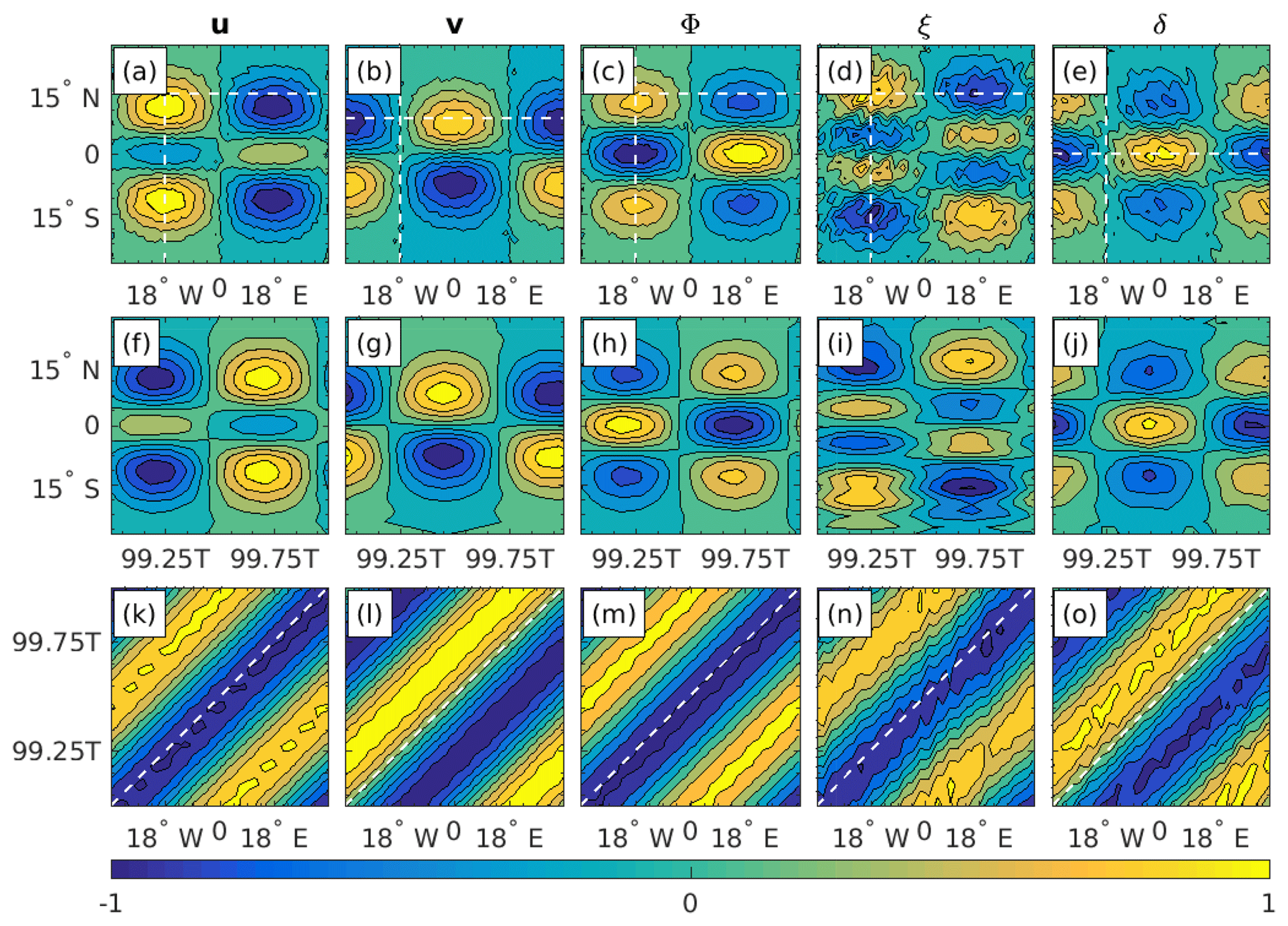
Figure 1 shows the initial u, v, Φ, ξ, and δ fields (where ξ and δ are the relative vorticity and divergence, respectively) of the chosen Rossby wave mode (Fig. 1a–e), and the resulting latitude–time (Fig. 1f–j) and time–longitude (Fig. 1k–o) Hovmöller diagrams of the simulated solution. The initial fields were obtained using the analytic expressions from Sect. 2 and the wave parameters from Sect. 3.1. The simulated solutions were obtained using the abovementioned equatorial channel model. The chosen intersects used in the calculation of the Hovmöller diagrams are indicated by white dashed lines superimposed on the initial fields, and are also provided in the figure's caption. For the sake of legibility the time domain shown in each panel is only the last wave period of the simulation, i.e., , where T is the wave period. The fields are normalized on their global maximum at t=0. Thus, white regions correspond to times at which the simulated solution exceeds the initial wave amplitude, momentarily. With this in mind, recall that the patterns in the latitude–time diagrams are similar to those in latitude–longitude diagrams, and can therefore be used for comparison with the initial fields. In general, the initial wave structure is preserved and the dominant slope in the time–longitude diagrams corresponds to the analytic slope indicated by dashed white lines (Fig. 1k–o). There are, however, some noticeable deviations: a slight east–west tilt can be observed in the latitude–time diagrams (Fig. 1f–j), but most egregiously, the divergence field is less regular than the other four. We return to this last point at the end of Sect. 4.3. The phase of the simulated patterns in the latitude–time diagrams fit the expected patterns considering the westward propagation of the Rossby mode at in 1 wave period after 99 wave periods.
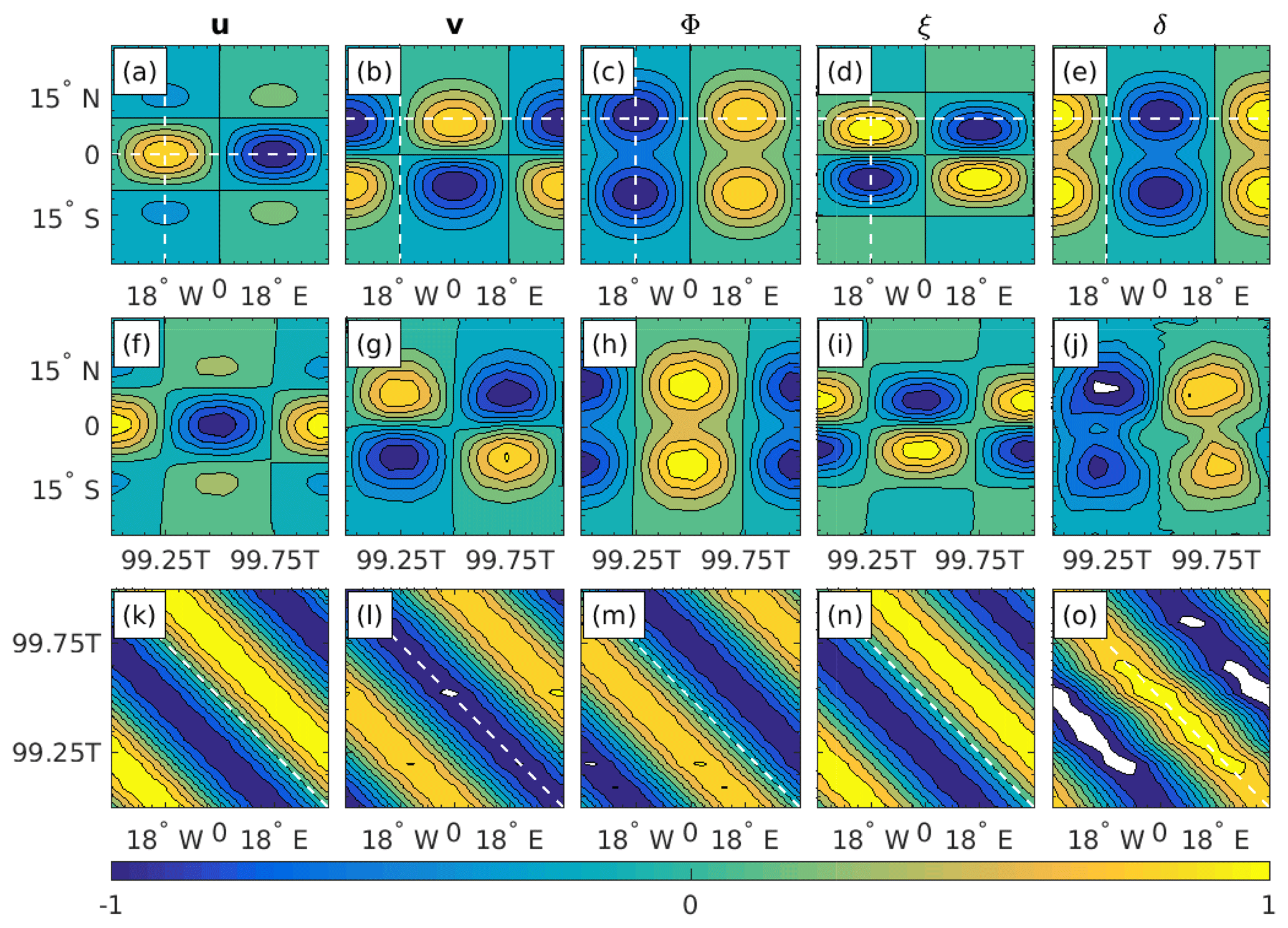
Figure 1(a–e) The initial u, v, Φ, ξ, and δ Rossby wave fields, obtained using the analytic expressions from Sect. 2 and the wave parameters from Sect. 3.1. (f–j) Latitude–time Hovmöller diagrams of the simulated solutions, obtained by intersecting the fields at (also indicated by the white vertical dashed lines in a–e). (k–o) Time–longitude Hovmöller diagrams of the simulated solutions, obtained by intersecting u at and all other fields at (also indicated by the white horizontal dashed lines in a–e). The simulated solutions were obtained using the equatorial channel finite-difference model. The fields are normalized on their global maximum at t=0. The wave period for the chosen wave parameters is T=18.5 d. Contour levels range from −1.0 to +1.0 in intervals of 0.2.

Figure 2(a–e) The initial , ξ, and δ EIG wave fields, obtained using the analytic expressions from Sect. 2 and the wave parameters from Sect. 3.1. (f–j) Latitude–time Hovmöller diagrams of the simulated solutions, obtained by intersecting the fields at (also indicated by the white vertical dashed lines in a–e). (k–o) Time–longitude Hovmöller diagrams of the simulated solutions, obtained by intersecting v at , δ at and all other fields at (also indicated by the white horizontal dashed lines in a–e). The simulated solutions were obtained using the equatorial channel finite-difference model. The fields are normalized on their global maximum at t=0. The wave period for the chosen wave parameters is T=1.9 d. Contour levels range from −1.0 to +1.0 in intervals of 0.2.
Similarly, Fig. 2 shows the initial u, v, Φ, ξ, and δ fields of the chosen EIG wave mode (Fig. 2a–e), and the resulting latitude–time (Fig. 2f–j) and time–longitude (Fig. 2k–o) Hovmöller diagrams of the simulated solution. Note that under the normalization used here the initial v field is independent of the wave type and is therefore identical to the one in Fig. 1. In contrast to Fig. 1 the patterns in the latitude–time diagrams of the simulated solutions are noticeably out of phase. However, considering the agreement between the dominant slope in the time–longitude diagrams and the analytic slope indicated by the dashed white lines (Fig. 2k–o), it is reasonable to say that this phase shift only results from a small phase speed error that accumulates over time. In addition, in contrast to the Rossby wave in Fig. 1, the divergence field in this case is just as regular as the other four fields.
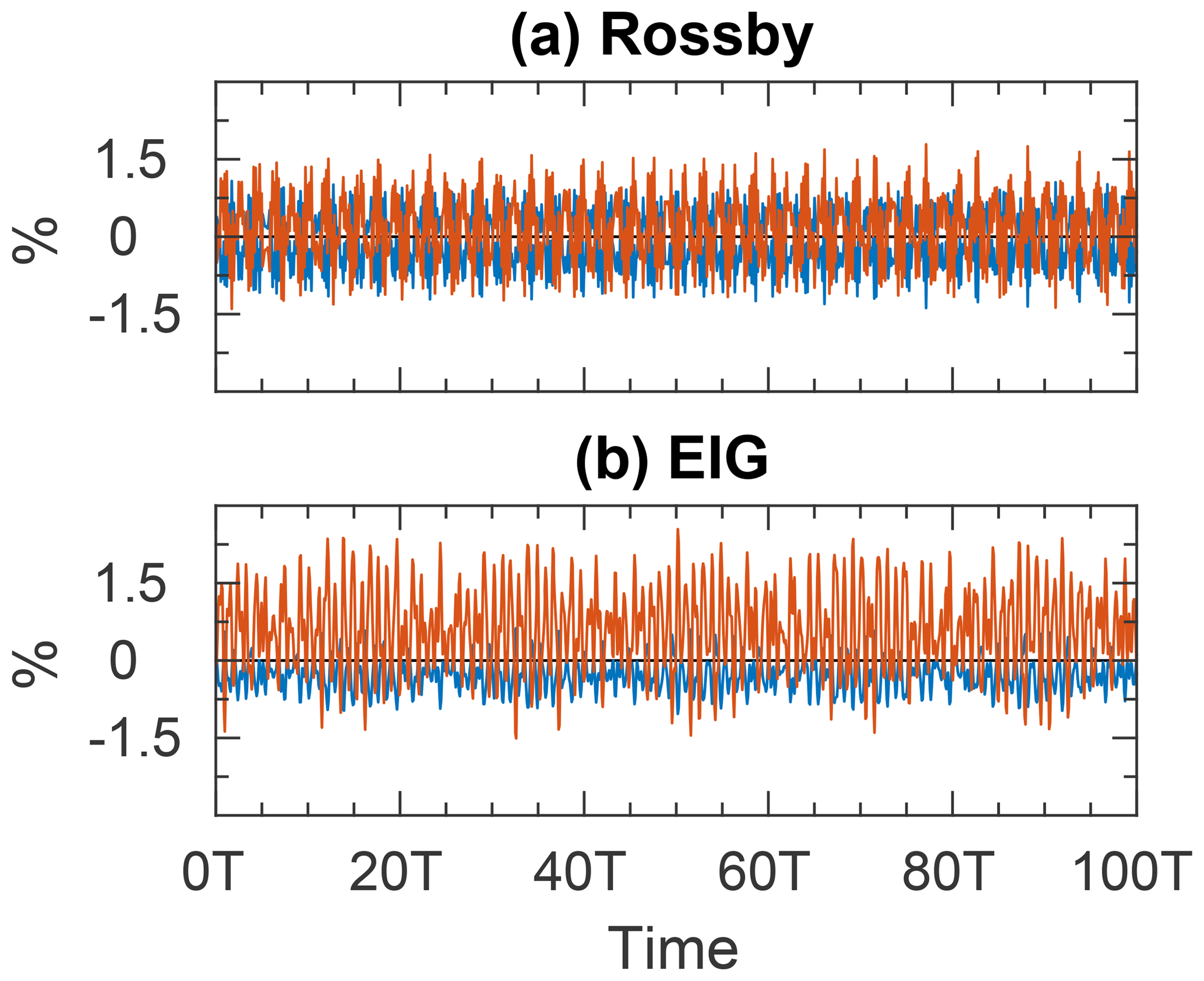
The structure error defined in Eq. (8) is shown in Fig. 3 for both Rossby (Fig. 3a) and EIG (Fig. 3b) waves as a function of time. In both cases the structure error fluctuates about a mean value of less than 1 % and there is no visible trend throughout the simulation time of 100 wave periods. Recall that the structure error defined in Eq. (8) is insensitive to phase differences.
4.2 Demonstration using a global-scale spectral model
To demonstrate the applicability of the Matsuno wave as a test case for global-scale models we use the Geophysical Fluid Dynamics Laboratory's (GFDL's) spectral transformed shallow-water model which uses spherical harmonics as its basis functions (https://www.gfdl.noaa.gov/idealized-spectral-models-quickstart/). The chosen spectral resolution was T85, i.e., a triangular truncation where both the highest retained wave number and the total wave number equal 85. The chosen time step was Δt=600 s, as in the equatorial channel model. The model contains provisions for hyper-diffusion terms as well as a temporal Robert–Asselin filter, but the coefficients of both were set to zero for the simulations described below.

Figure 4(a–e) The initial u, v, Φ, ξ, and δ Rossby wave fields, obtained using the analytic expressions from Sect. 2 and the wave parameters from Sect. 3.1. (f–j) Latitude–time Hovmöller diagrams of the simulated solutions, obtained by intersecting the fields at (also indicated by the white vertical dashed lines in a–e). (k–o) Time–longitude Hovmöller diagrams of the simulated solutions, obtained by intersecting u at and all other fields at (also indicated by the white horizontal dashed lines in a–e). The simulated solutions were obtained using GFDL's global-scale spectral model. The fields are normalized on their global maximum at t=0. The wave period for the chosen wave parameters is T=18.5 d. Contour levels range from −1.0 to +1.0 in intervals of 0.2.
Figure 4 shows the initial u, v, Φ, ξ, and δ fields (where ξ and δ are the relative vorticity and divergence, respectively) of the chosen Rossby wave mode (Fig. 4a–e), and the resulting latitude–time (Fig. 4f–j) and time–longitude (Fig. 4k–o) Hovmöller diagrams of the simulated solution. The initial fields were obtained using the analytic expressions from Sect. 2 and the wave parameters from Sect. 3.1. The simulated solutions were obtained using the abovementioned GFDL global-scale spectral model. The chosen intersects used in the calculation of the Hovmöller diagrams are indicated by white dashed lines superimposed on the initial fields, and are also provided in the figure's caption. For the sake of legibility the time domain shown in each panel is only the last wave period of the simulation, i.e., , where T is the wave period. The fields are normalized on their global maximum at t=0. Thus, white regions correspond to times at which the simulated solution exceeds the initial wave amplitude, momentarily. With this in mind, recall that the patterns in the latitude–time diagrams are similar to those in latitude–longitude diagrams, and can therefore be used for comparison with the initial fields. Indeed, the patterns in the latitude–time diagrams of the simulated solutions agree quite accurately with those of the initial wave structure, but are noticeably out of phase. Nevertheless, considering the agreement between the dominant slope in the time–longitude diagrams and the analytic slope indicated using the dashed white lines (Fig. 4k–o), it is reasonable to say that this phase shift results from a small phase speed error that accumulates over time. In addition, the divergence field is less regular than the other four fields. We return to this point at the end of Sect. 4.3.
Similarly, Fig. 5 shows the initial u, v, Φ, ξ, and δ fields of the chosen EIG wave mode (Fig. 5a–e), and the resulting latitude–time (Fig. 5f–j) and time–longitude (Fig. 5k–o) Hovmöller diagrams of the simulated solution. Note that under the normalization used in the present paper the initial v field is independent of the wave type and is therefore identical to the one in Fig. 4. As in Fig. 4, the patterns in the latitude–time diagrams of the simulated solutions are noticeably out of phase, but the dominant slope in the time–longitude diagrams (Fig. 5k–o) agrees well with the analytic slope, indicating that the observed phase shift results from a small phase speed error that accumulates over time.
Finally, the structure error in Fig. 6 fluctuates about a mean value of less than 1 % and there are no visible trends throughout the 100 wave period simulations. Recall that the structure error defined in Eq. (8) is insensitive to phase differences.
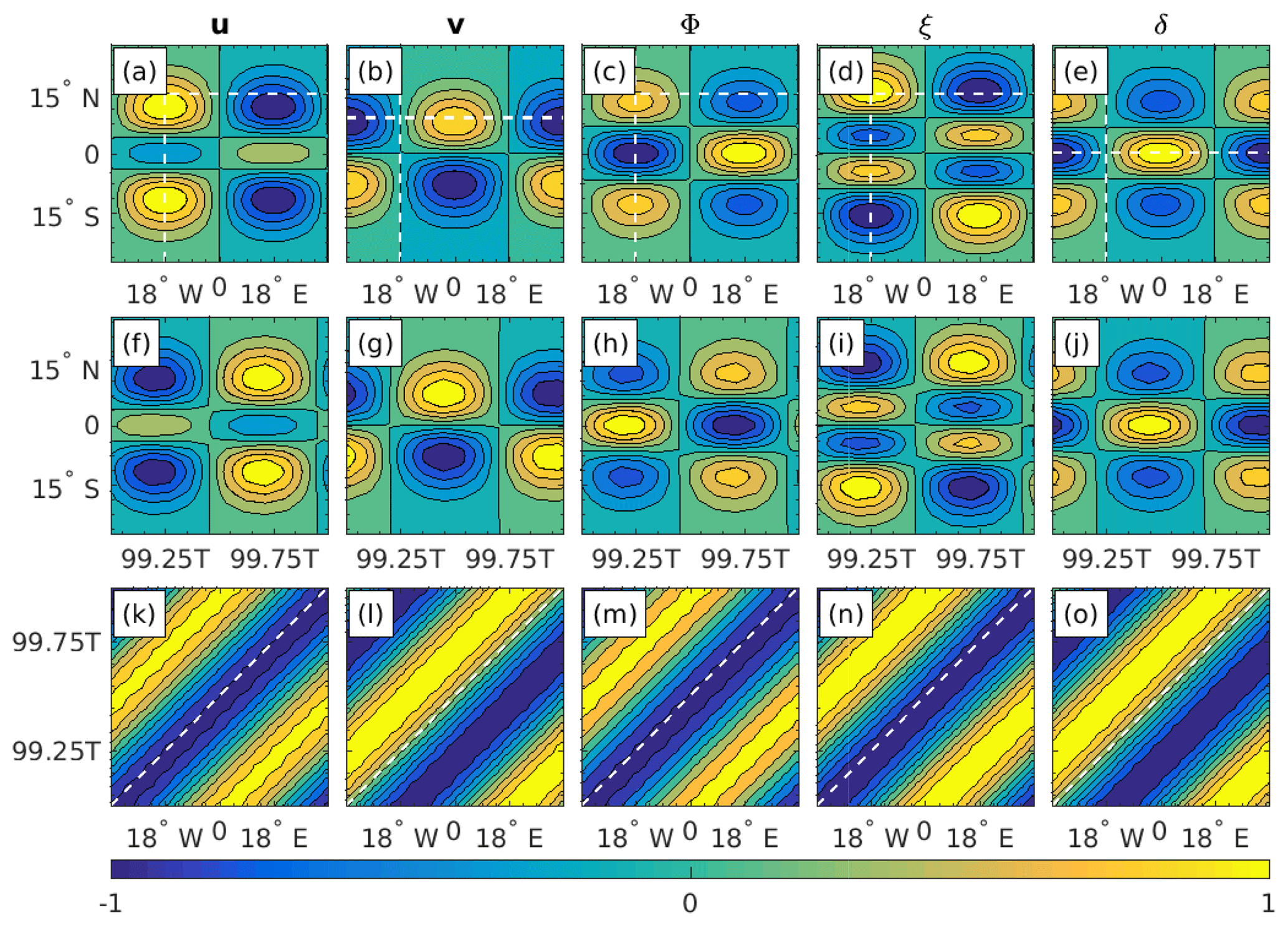
Figure 5(a–e) The initial u, v, Φ, ξ, and δ EIG wave fields, obtained using the analytic expressions from Sect. 2 and the wave parameters from Sect. 3.1. (f–j) Latitude–time Hovmöller diagrams of the simulated solutions, obtained by intersecting the fields at (also indicated by the white vertical dashed lines in a–e). (k–o) Time–longitude Hovmöller diagrams of the simulated solutions, obtained by intersecting v at , δ at and all other fields at (also indicated by the white horizontal dashed lines in a–e). The simulated solutions were obtained using the GFDL global-scale spectral model. The fields are normalized on their global maximum at t=0. The wave period for the chosen wave parameters is T=1.9 d. Contour levels range from −1.0 to +1.0 in intervals of 0.2.

4.3 Smoothness and stability
In this section we examine the generation of small-scale features and the stability of the proposed wave solutions in a similar fashion to that used in Thuburn and Li (2000) for the original Rossby–Haurwitz wave number 4.
In Thuburn and Li (2000), the generation of small-scale features and the potential enstrophy cascade is observed by examining the potential vorticity field, which generates tongues that wrap up around themselves and break the initial east–west symmetry. For the small wave amplitude m s−1 used in the present work, the potential vorticity is dominated by the planetary vorticity which is 5–6 orders of magnitude (depending on the wave) larger than the relative vorticity. Thus, instead of the potential vorticity we examine the relative vorticity (as well as the geopotential). Figures 1–2, as well as Figs. 4–5, show the evolution of these two fields between t=99T and t=100T, where T is the wave period in each case. Clearly, both fields remain regular throughout the simulations and do not develop small-scale features such as those observed in Thuburn and Li (2000). Recall that the simulations in the present work were carried out without any diffusion/viscosity terms. Thus, the simulations remain stable for at least 100 wave periods with no need to remove potential enstrophy at the grid scale.
In order to examine the stability of the chosen initial waves we repeat the simulations of the previous section with an added perturbation (white noise) to the initial fields. We demonstrate the stability of the waves using only the global-scale model, which was found to yield more stable results when adding the perturbation.
Figures 7 and 8 show the initial fields of the perturbed Rossby (Fig. 7a–e) and EIG waves (Fig. 8a–e), respectively, and the resulting latitude–time (Figs. 7f–j and 8f–j) and time–longitude (Figs. 7k–o and 8k–o) Hovmöller diagrams of the simulated solution, obtained using the GFDL global-scale spectral model. The initial perturbation in these figures consist of a uniformly distributed random white noise with an amplitude of 5 % of the field's amplitude added to each of the fields u, v, and Φ. Specifically, let q stand for any of the variables u, v or Φ, then the initial perturbation is given by
where qa is the analytic solutions obtained as in Sect. 2, and R is a uniformly sampled random array with elements in (0,1) whose dimensions are the same as qa (in the present work a different R was drawn for each of the three variables).
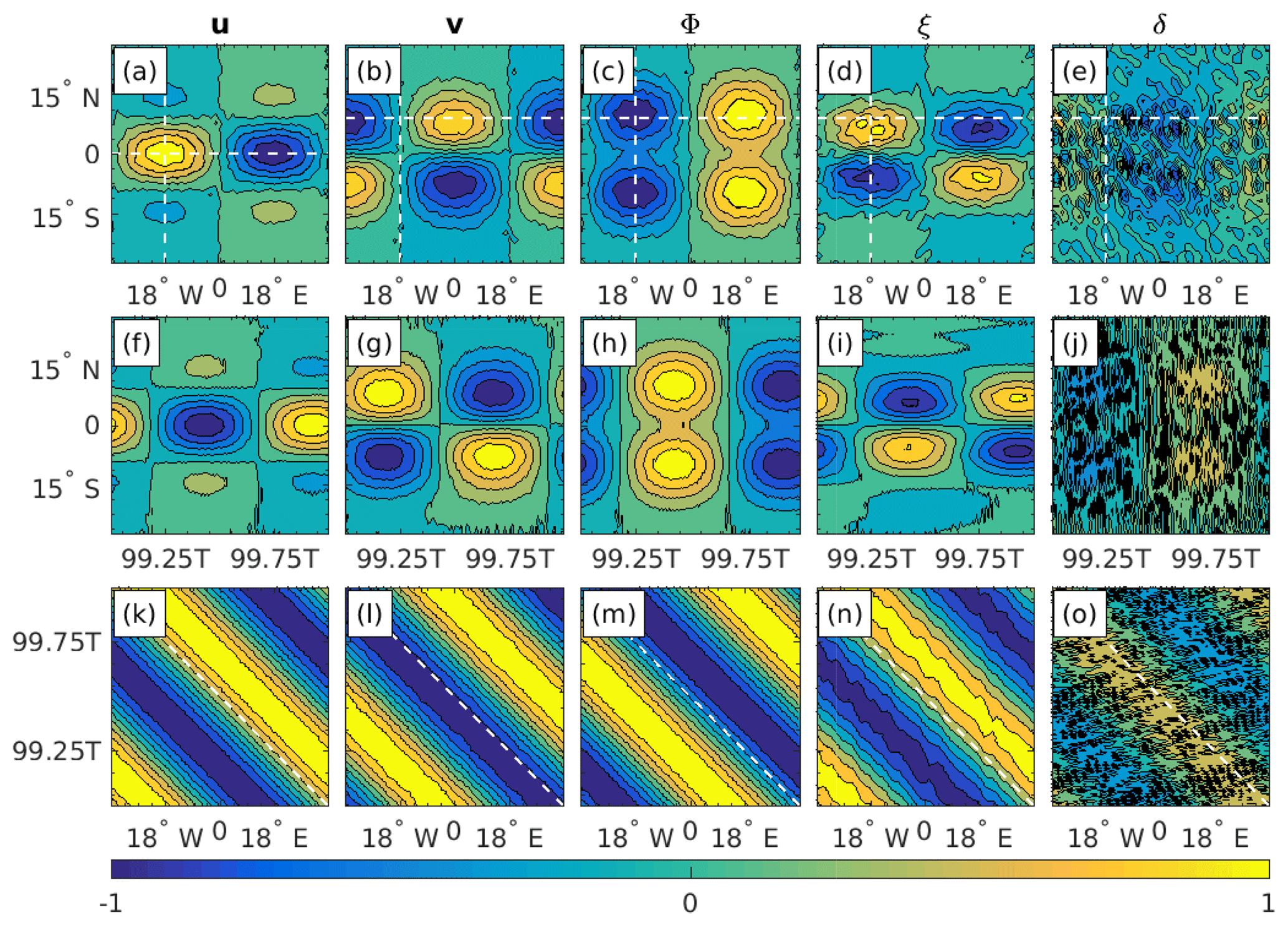
Overall, the perturbed waves seem to be stable. The u, v and Φ fields are almost as regular as those of the non-perturbed waves, except for the zero contour. The small-scale features in the vorticity field of the perturbed Rossby wave smooth out with time, in contrast to the potential vorticity field of the Rossby–Haurwitz wave number 4. Conversely, the perturbed Rossby wave divergence field is completely eroded. The vorticity and divergence fields of the perturbed EIG wave are not as regular as those of the non-perturbed wave. However, they too become smoother with time and the initial wave remains the most dominant wave throughout the entire 100 wave period simulation. The structure error in Fig. 9 is similar to the previous ones in Figs. 3 and 6. These results are quite surprising, as we would expect a sufficiently large perturbation to excite other modes, regardless of the waves' stability.

Both the non-perturbed Rossby wave in Sect. 4.1 and 4.2, and the perturbed Rossby wave in the present section indicate that the divergence field is more sensitive than the other four fields of the Rossby wave. An immediate suspect in this regard is the divergence field amplitude, which is small for the chosen Rossby wave. For reference, the meridional wind amplitude for the chosen waves parameters (of both the Rossby and EIG waves) is , whereas the Rossby wave divergence field amplitude is . Conversely, the divergence field amplitude is only 1 order of magnitude smaller than the vorticity field amplitude, which is . Regardless of the cause, the fact that all other four fields remain quite regular while the divergence field is completely eroded suggests that the small but significant divergence field described by Phillips (1959) is in fact a small and insignificant divergence field.
4.4 Convergence test for the linear shallow-water models
In addition to the test cases proposed by Williamson et al. (1992) a resolution convergence test of linearized SWEs in which the simulations are compared to higher-order simulations is also useful for ensuring that the errors decrease with the increase in resolution. In this section we demonstrate that Matsuno's analytic wave solutions can be used for this purpose. We use the equatorial channel model which can be easily turned into a linear shallow-water model.
Figure 10 shows the structure error in absolute value as a function of the grid spacing , from to every 0.25∘. For each resolution, the initial non-perturbed waves were integrated for 100 wave periods. As an estimate of the structure error at each resolution we use the time-series averages (indicated by dots). The error bars were estimated using the standard deviations of the entire time series. As the resolution increases from to , the structure error time-series average decreases from about 2 % to less than 1 %, and the standard deviation decreases from about 2 % to about 0.5 %. The time step across all resolutions in this figure was held fixed at Δt=100 s. Note that all of the results of the previous sections were obtained for and Δt=600 s. This time step was found to yield convergent results for in the sense that decreasing the time step by a factor of 2 yields no improvements. Nevertheless, for the convergence test in the present section we have further decreased the time step to Δt=100 s in order to allow a further increase in the spatial resolution by another 0.25∘. This has also enabled a comparison with the results of the previous sections, thus ensuring that the simulations remain stable. Needless to say, for any time step one can expect to encounter numerical instabilities at some (high) spatial resolution.

Figure 10Structure error in absolute value as a function of the grid spacing , from to every 0.25∘. The points correspond to the time averaged structure error over 100 wave periods, and the error bars are determined from the standard deviation. Blue: calculated for the velocity vector . Red: calculated for the geopotential Φ.
As vertical resolutions in atmospheric and oceanic models increase it is essential to assess the accuracy with which they resolve baroclinic wave modes, typified by low gravity-wave phase speeds, in addition to the barotropic mode. To this end we propose to use a similar procedure to that used in the Rossby–Haurwitz test case but with different initial conditions. Instead of using the analytic solutions obtained by Haurwitz (1940), which are only accurate for high gravity-wave speeds such as those of the barotropic mode, we propose the use of the analytic solutions obtained by Matsuno (1966), which are accurate for lower gravity-wave speeds such as those of the baroclinic modes.
While the solutions from Matsuno (1966) apply for the equatorial β-plane, they approximate the solutions of the SWEs on the sphere for the speeds of gravity waves found in the baroclinic modes in the atmosphere, and as demonstrated in the present work can be accurately simulated in both equatorial channel and global-scale models in spherical coordinates. In addition, unlike the original Rossby–Haurwitz wave number 4, the chosen initial waves of the present test case remain stable for at least 100 wave periods, which for the chosen Rossby wave correspond to about 1850 d.
While the solutions of the SWEs obtained by Matsuno (1966) account for the small divergence field missing from the non-divergent Rossby–Haurwitz waves, the results of the present study suggest that this missing divergence field is insignificant.
Ideally, we expect the proposed test case to stand on an equal footing alongside the Rossby–Haurwitz test case, but in the words of Williamson et al. (1992): “The test will only become standard to the extent that the community finds it useful”.
A Python module for evaluating the initial conditions and analytic solutions is publicly available under the MIT license at https://github.com/ofershamir/matsuno and archived on Zenodo at https://doi.org/10.5281/zenodo.2605203.
NP conceived the idea of standardizing the Matsuno test case for general circulation models in spherical coordinates. IY adopted the Cartesian shallow-water model used in Gildor et al. (2016) to spherical coordinates and was responsible for the numerical simulations. OS analyzed the numerical results, prepared the paper and ran the GFDL spectral global model. SZZ prepared the IC generating code for packaging, deployment, testing and licensing.
The authors declare that they have no conflict of interest.
Haim Zvi Krugliak and Chaim Israel Garfinkel of HU helped us install and run the GFDL model. We also acknowledge the helpful discussions we had with Yair De-Leon of HU and the insightful comments of the two anonymous reviewers of our paper.
This paper was edited by David Ham and reviewed by two anonymous referees.
Abramowitz, M. and Stegun, I. A.: Handbook of Mathematical Functions with Formulas, Graphs, and Mathematical Tables, National Bureau of Standards, Applied Mathematics Series, Dover, 56, 1046 pp., 1964. a
Bosler, P., Wang, L., Jablonowski, C., and Krasny, R.: A Lagrangian particle/panel method for the barotropic vorticity equations on a rotating sphere, Fluid Dyn. Res., 46, 031406, https://doi.org/10.1088/0169-5983/46/3/031406, 2014. a
De-Leon, Y. and Paldor, N.: Zonally propagating wave solutions of Laplace Tidal Equations in a baroclinic ocean of an aqua-planet, Tellus A, 63, 348–353, https://doi.org/10.1111/j.1600-0870.2010.00490.x, 2011. a, b
Garfinkel, C. I., Fouxon, I., Shamir, O., and Paldor, N.: Classification of eastward propagating waves on the spherical Earth, Q. J. Roy. Meteor. Soc., 143, 1554–1564, 2017. a, b, c
Gildor, H., Paldor, N., and Ben-Shushan, S.: Numerical simulation of harmonic, and trapped, Rossby waves in a channel on the midlatitude β-plane, Q. J. Roy. Meteor. Soc., 142, 2292–2299, 2016. a, b
Haurwitz, B.: The motions of the atmospheric disturbances on the spherical earth, J. Mar. Res., 3, 254–267, 1940. a, b, c, d
Hoskins, B. J.: Stability of the Rossby-Haurwitz wave, Q. J. Roy. Meteor. Soc., 99, 723–745, https://doi.org/10.1002/qj.49709942213, 1973. a
Jablonowski, C.: Adaptive grids in weather and climate modeling, PhD thesis, University of Michigan, Ann Arbor, MI, USA, 2004. a
Jablonowski, C. and Williamson, D. L.: A baroclinic instability test case for atmospheric model dynamical cores, Q. J. Roy. Meteor. Soc., 132, 2943–2975, 2006. a
Jablonowski, C., Oehmke, R. C., and Stout, Q. F.: Block-structured adaptive meshes and reduced grids for atmospheric general circulation models, Philos. T. Roy. Soc. A, 367, 4497–4522, 2009. a
Lauritzen, P. H., Jablonowski, C., Taylor, M. A., and Nair, R. D.: Rotated versions of the Jablonowski steady-state and baroclinic wave test cases: A dynamical core intercomparison, J. Adv. Model. Earth Syst., 2, 15, https://doi.org/10.3894/JAMES.2010.2.15, 2010. a
Li, X., Peng, X., and Li, X.: An improved dynamic core for a non-hydrostatic model system on the Yin-Yang grid, Adv. Atmos. Sci., 32, 648–658, 2015. a
Matsuno, T.: Quasi-geostrophic motions in the equatorial area, J. Meteorol. Soc. Jpn., Ser. II, 44, 25–43, 1966. a, b, c, d, e, f, g, h, i, j, k, l, m, n, o, p
Mohammadian, A. and Marshall, J.: A “vortex in cell” model for quasi-geostrophic, shallow water dynamics on the sphere, Ocean Model., 32, 132–142, 2010. a
Paldor, N., De-Leon, Y., and Shamir, O.: Planetary (Rossby) waves and inertia–gravity (Poincaré) waves in a barotropic ocean over a sphere, J. Fluid Mech., 726, 123–136, 2013. a, b, c
Paldor, N., Fouxon, I., Shamir, O., and Garfinkel, C. I.: The mixed Rossby–gravity wave on the spherical Earth, Q. J. Roy. Meteor. Soc., 144, 1820–1830, https://doi.org/10.1002/qj.3354, 2018. a
Phillips, N. A.: Numerical integration of the primitive equations on the hemisphere, Mon. Weather Rev., 87, 333–345, https://doi.org/10.1175/1520-0493(1959)087<0333:NIOTPE>2.0.CO;2, 1959. a, b, c, d
Polvani, L. M., Scott, R., and Thomas, S.: Numerically converged solutions of the global primitive equations for testing the dynamical core of atmospheric GCMs, Mon. Weather Rev., 132, 2539–2552, 2004. a, b
Press, W. H., Teukolsky, S. A., Vetterling, W. T., and Flannery, B. P.: Numerical recipes, 3rd edn., The art of scientific computing, Cambridge University Press, New York, 2007. a
Shamir, O. and Paldor, N.: A quantitative test case for global-scale dynamical cores based on analytic wave solutions of the shallow-water equations, Q. J. Roy. Meteor. Soc., 142, 2705–2714, 2016. a, b, c
Thuburn, J. and Li, Y.: Numerical simulations of Rossby–Haurwitz waves, Tellus A, 52, 181–189, 2000. a, b, c, d, e, f, g
Ullrich, P. A.: A global finite-element shallow-water model supporting continuous and discontinuous elements, Geosci. Model Dev., 7, 3017–3035, https://doi.org/10.5194/gmd-7-3017-2014, 2014. a
Ullrich, P. A., Melvin, T., Jablonowski, C., and Staniforth, A.: A proposed baroclinic wave test case for deep-and shallow-atmosphere dynamical cores, Q. J. Roy. Meteor. Soc., 140, 1590–1602, 2014. a
Wheeler, M. and Kiladis, G. N.: Convectively coupled equatorial waves: Analysis of clouds and temperature in the wavenumber–frequency domain, J. Atmos. Sci., 56, 374–399, 1999. a, b, c
Williamson, D. L., Drake, J. B., Hack, J. J., Jakob, R., and Swarztrauber, P. N.: A standard test set for numerical approximations to the shallow water equations in spherical geometry, J. Comput. Phys., 102, 211–224, https://doi.org/10.1016/S0021-9991(05)80016-6, 1992. a, b, c, d