the Creative Commons Attribution 4.0 License.
the Creative Commons Attribution 4.0 License.
 | 14 Jan 2019
Implementation and performance of adaptive mesh refinement in the Ice Sheet System Model (ISSM v4.14)
Thiago Dias dos Santos
Mathieu Morlighem
Hélène Seroussi
Philippe Remy Bernard Devloo
Jefferson Cardia Simões
Accurate projections of the evolution of ice sheets in a changing climate require a fine mesh/grid resolution in ice sheet models to correctly capture fundamental physical processes, such as the evolution of the grounding line, the region where grounded ice starts to float. The evolution of the grounding line indeed plays a major role in ice sheet dynamics, as it is a fundamental control on marine ice sheet stability. Numerical modeling of a grounding line requires significant computational resources since the accuracy of its position depends on grid or mesh resolution. A technique that improves accuracy with reduced computational cost is the adaptive mesh refinement (AMR) approach. We present here the implementation of the AMR technique in the finite element Ice Sheet System Model (ISSM) to simulate grounding line dynamics under two different benchmarks: MISMIP3d and MISMIP+. We test different refinement criteria: (a) distance around the grounding line, (b) a posteriori error estimator, the Zienkiewicz–Zhu (ZZ) error estimator, and (c) different combinations of (a) and (b). In both benchmarks, the ZZ error estimator presents high values around the grounding line. In the MISMIP+ setup, this estimator also presents high values in the grounded part of the ice sheet, following the complex shape of the bedrock geometry. The ZZ estimator helps guide the refinement procedure such that AMR performance is improved. Our results show that computational time with AMR depends on the required accuracy, but in all cases, it is significantly shorter than for uniformly refined meshes. We conclude that AMR without an associated error estimator should be avoided, especially for real glaciers that have a complex bed geometry.
- Article
(7024 KB) - Full-text XML
-
Supplement
(77551 KB) - BibTeX
- EndNote


The uncertainty in projections of ice sheet contribution to sea level rise in the next century remains large, primarily due to the potential collapse of the West Antarctic Ice Sheet (Church et al., 2013; DeConto and Pollard, 2016; Jevrejeva et al., 2014; Ritz et al., 2015). Projections of the collapse of WAIS are based on the marine ice sheet instability (MISI) hypothesis (Mercer, 1978; Thomas, 1979; Weertman, 1974). This hypothesis refers to ice sheets grounded below sea level on retrograde bedrock slopes (as seen in Fig. 1), as is the case for many glaciers in WAIS (Fretwell et al., 2013). MISI states that the grounding line (GL), the region where the ice sheet starts to float (see Fig. 1), cannot remain stable on such bedrock slopes (Gudmundsson et al., 2012; Katz and Worster, 2010; Schoof, 2007b). Accordingly, the GL retreat on retrograde bedrock slopes causes increased ice discharge, which in turn leads to further GL retreat, resulting in a non-linear positive feedback. This self-sustaining GL retreat persists until a prograde bedrock slope is reached. Therefore, a change in climate or ocean can potentially force a large-scale fast migration of the GL inland (Favier et al., 2014; Schoof, 2007a; Seroussi et al., 2014b). Recently, WAIS has experienced an increase in the intrusion of ocean warm deep water (Dutrieux et al., 2014; Jacobs et al., 2011) that likely increased the ocean-induced melt under ice shelves, reduced the buttressing they provide to inland ice and triggered the retreat of grounding lines around WAIS observed over the last decades (Christie et al., 2016; Kimura et al., 2016; Rignot et al., 2014; Seroussi et al., 2017).
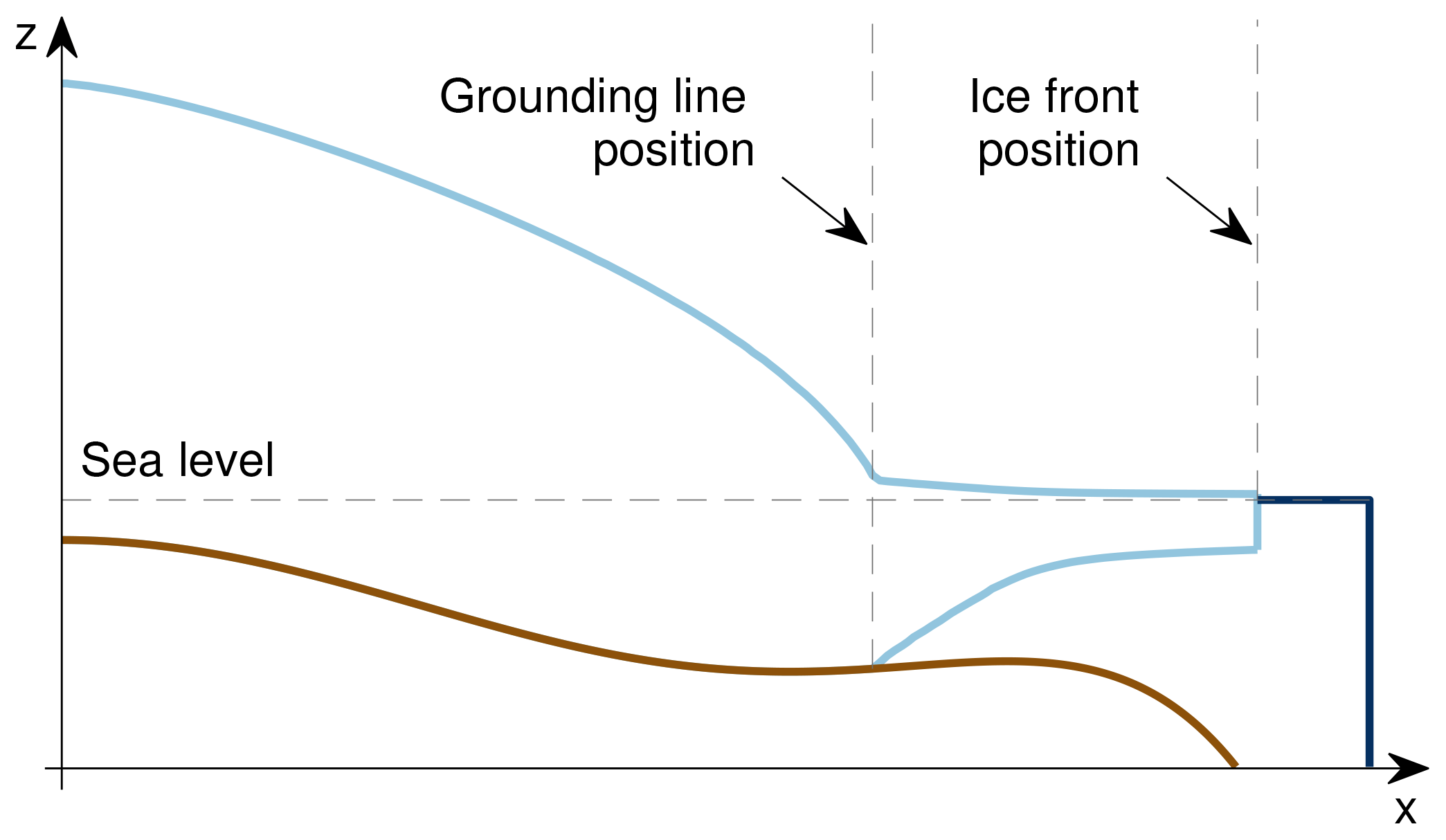
Figure 1Vertical cross-section of a marine ice sheet: marine ice sheet (light blue), ocean (dark blue) and bedrock (brown). The position of the grounding line is implicitly defined by the level set function, ϕgl, based on a hydrostatic floatation criterion (Seroussi et al., 2014a).
Modeling this positive feedback requires the coupling of different physical processes (ice sheet and ice shelf evolutions, GL migration, basal friction, etc.), and the accuracy of the result is highly dependent on the GL parameterization and the spatial discretization of the domain. Vieli and Payne (2005) compared the results of different ice sheet numerical models in terms of GL migration and found that the numerical results have a strong dependency on horizontal grid size. Analyzing the stability and dynamics of the GL on reverse bed slopes, Schoof (2007b) pointed out that sufficiently high grid resolution in the GL zone is a critical element to obtain reliable numerical results. Two ice sheet model intercomparison projects (MISMIP and MISMIP3d) later confirmed the GL dynamics dependency on spatial resolutions (Pattyn et al., 2012, 2013).
Several marine ice sheet models have employed different numerical schemes to overcome this mesh resolution requirement at the GL with reduced computational cost: by imposing a flux condition at the GL position (Pattyn, 2017; Pollard and DeConto, 2009, 2012), by treating the GL and basal friction with sub-grid or sub-element schemes (Feldmann et al., 2014; Leguy et al., 2014; Seroussi et al., 2014a) or by applying high spatial resolution only in the GL region with adaptive grid refinement (Cornford et al., 2013; Durand et al., 2009; Gladstone et al., 2010; Goldberg et al., 2009; Gudmundsson et al., 2012).
The grid or mesh adaptation technique allows resources to be applied only where they are required, which is very useful in transient simulations that include some discontinuity in the time-dependent solution (Berger and Colella, 1989; Devloo et al., 1987), as is the case for GL dynamics as defined in Schoof (2007b), as the basal friction is only applied to grounded ice. This technique can be performed with two different methods: r-adaptivity and h-adaptivity methods (Oden et al., 1986). The r-adaptivity method, also known as moving mesh method, moves progressively a fixed number of vertices in a given direction or region (Anderson et al., 1984), while the h-adaptivity method, named in this work as adaptive mesh refinement (AMR), splits edges and/or elements, inserting new vertices into the mesh where high resolution is required (Berger and Colella, 1989; Devloo et al., 1987). The performance of each of these methods depends on the problem for which they are applied. Vieli and Payne (2005) showed that models applying a moving grid to track the GL movement perform better than fixed grid models. Since the position of the GL is explicitly defined in moving grids, Vieli and Payne (2005) noticed for this method a weak grid resolution dependency in comparison to the fixed grid method, for which the GL position falls between grid points. Goldberg et al. (2009) obtained accurate solutions with fewer resources solving the time-dependent shelfy-stream equations with the two different mesh adaptation techniques mentioned above, moving mesh and AMR. Using a one-dimensional shelfy-stream model based on finite difference scheme, Gladstone et al. (2010) demonstrated that AMR and sub-grid parameterization for GL position could produce robust predictions of GL migration. Pattyn et al. (2012) found that moving grid methods tend to be the most accurate and AMR can further improve accuracy compared to models based on a fixed grid. Cornford et al. (2013) implemented a block-structured AMR in the Berkeley Ice Sheet Initiative for Climate Extremes (BISICLES), a 2.5-D ice sheet model based on the finite volume method. They demonstrated that simulations with AMR are computationally cheaper and more efficient, even as the grounding line moves over significant distances. Jouvet and Gräser (2013) combined the shallow ice approximation and the shallow-shelf approximation in an AMR numerical scheme involving a truncated Newton multigrid and finite volume method. Through MISMIP3d experiments (Pattyn et al., 2013), they highlighted the relevance and efficiency of AMR in terms of computational cost when high resolution (∼100 m) is necessary to reproduce GL reversibility. Recently, Gillet-Chaulet et al. (2017) implemented an anisotropic mesh adaptation in the finite element ice flow model, Elmer/Ice (Gagliardini et al., 2013). Based on the MISMIP+ experiment (Asay-Davis et al., 2016), they showed that combining various variables (ice thickness, basal drag, velocity, etc.) in an estimator allowed to reduce the number of mesh vertices by more than 1 order of magnitude compared to uniformly refined meshes, for the same level of numerical accuracy.
Here, we implement the AMR technique for unstructured meshes in the parallel finite element Ice Sheet System Model (Larour et al., 2012). The AMR capability in ISSM relies on two different and independent mesh generators (one or the other mesh generator is used according to the user's choice): Bamg, a bi-dimensional anisotropic mesh generator developed by Hecht (2006), and NeoPZ, a finite element library developed by Devloo (1997). ISSM's architecture is based on the Message Passing Interface (MPI), where models are run in a distributed memory scheme. Our AMR implementation minimizes MPI communications, avoiding overheads and latencies. Since refinement criteria are crucial to AMR performance (Devloo et al., 1987), we implement different criteria based on (a) the distance to the grounding line, (b) the Zienkiewicz–Zhu (ZZ) error estimator (Zienkiewicz and Zhu, 1987) and (c) different combinations of (a) and (b). To analyze the performance of AMR, we run two benchmark experiments: MISMIP3d (Pattyn et al., 2013) and MISMIP+ (Asay-Davis et al., 2016). We compare AMR results from both Bamg and NeoPZ with uniformly refined meshes in terms of GL position and computational time.
This paper is organized as follows: in Sect. 2, we summarize the main features of ISSM's architecture and the strategies used to implement an efficient AMR technique for transient simulations. In Sect. 3, we describe both MIMISP3d and MISMIP+ experiments used to analyze the AMR performance, and in Sect. 4 we present the results in terms of GL position and processing time. We finish this paper with a discussion of the results and conclusions in Sects. 5 and 6, respectively.
2.1 ISSM architecture
Our AMR implementation is strongly based on the architecture of ISSM. We describe here the main ISSM features necessary to understand the AMR strategy. We refer to Larour et al. (2012) for a more detailed description of ISSM.
Several stress balance approximations are implemented in ISSM, including higher-order models (Pattyn, 2003). The current AMR capability is supported for the 2-D vertically integrated shallow-shelf or shelfy-stream approximation (MacAyeal, 1989; Morland, 1987). The SSA is employed for both grounded and floating ice, so membrane stress terms (Schoof, 2007b) are included but all vertical shearing is neglected (Seroussi et al., 2014a). Here, the mesh used for the SSA equations is unstructured and relies on a Delaunay triangulation.
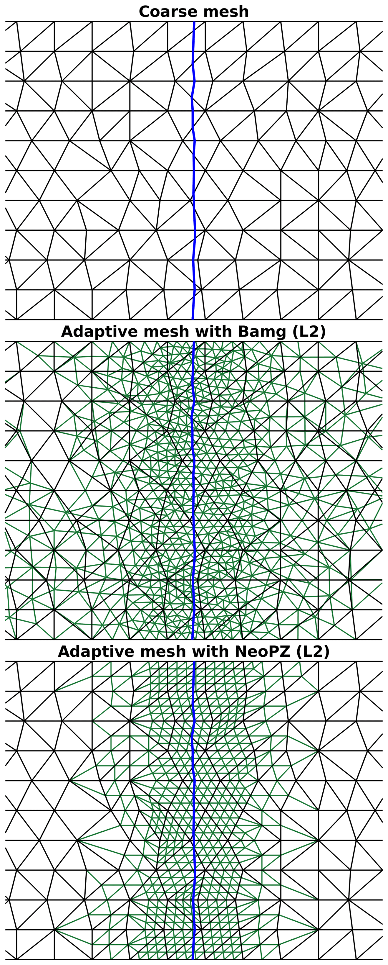
Figure 2Examples of adaptive meshes using Bamg and NeoPZ. Blue line: grounding line position. Black lines: coarse mesh, common for Bamg and NeoPZ. Green lines: adaptive meshes with level of refinement equal to 2 (L2). Bamg keeps vertices and connectivities unchanged as much as possible compared to the coarse mesh. NeoPZ generates nested meshes; vertices and connectivities of the coarse mesh are kept unchanged.
ISSM is designed to run in parallel in a distributed memory fashion by MPI. When a model is launched, the entire mesh is spatially partitioned over processing units or cores (CPUs), and data structures related to the finite element method are built in each partition. All physical entities that vary in space (ice viscosity, ice thickness, surface, velocities, etc.) are kept within the elements.
MPI communications between the partitions (CPUs) are performed to assemble the global stiffness matrix and load vector, as well as during the solution update in the elements once the system of equations is solved. The advantage of MPI is its ability to handle larger models (i.e., for continental-scale simulations) in many cores and nodes on a cluster. Its disadvantage is the cost in the communications between the partitions.
2.2 Bamg and NeoPZ
The AMR technique in ISSM is implemented for unstructured meshes and triangular elements. Here are some short descriptions of the mesh generators Bamg and NeoPZ.
Bamg (Hecht, 2006) is a bi-dimensional mesh generator based on Delaunay-like method (Hecht, 2005). This mesh generator is embedded in ISSM for static anisotropic mesh adaptation (Morlighem et al., 2010). Here, we extend Bamg capabilities for dynamic adaptation (AMR). The refinement in Bamg is carried out by specifying the desired resolution on the vertices. To reach the desired resolution, Bamg's algorithm splits triangle edges and inserts new vertices in the mesh (Hecht, 2006). The algorithm keeps new vertices and connectivities unchanged as much as possible compared to the previous mesh (Hecht, 2005). This procedure reduces the numerical errors introduced by the AMR when the solutions are interpolated into the new mesh (see Sect. 2.3). Regions of different resolutions are linked by a mesh transition zone, where the element sizes are changed gradually. The spatial extent of this mesh transition zone is also specified by the user in Bamg's algorithm. An example of adaptive mesh using Bamg is shown in Fig. 2.
NeoPZ (Devloo, 1997) is a finite element library dedicated to highly adaptive techniques (Calle et al., 2015). In NeoPZ's data structure, each element is refined into four topologically similar elements, whose resolutions are half of the refined element. To avoid hanging vertices (Calle et al., 2015), some elements are divided in specific ways such that any two elements in the mesh may have a vertex or an entire edge in common, or no vertices in common (Szabó and Babuška, 1991). In this sense, all meshes refined by NeoPZ are nested; i.e., vertices and connectivities from the coarse mesh are kept fixed during the entire simulation time. This characteristic does not introduce any numerical error induced by the AMR during the interpolation process (see Sect. 2.3). The AMR with NeoPZ is given by specifying the level of refinement, i.e., how often elements are refined. Therefore, the mesh transition zone, which links regions of different resolutions, is generated stepwise through resolutions dictated by levels of refinement. Figure 2 shows an example of an adaptive mesh using NeoPZ.
Here, we describe the algorithm to couple ISSM to Bamg and NeoPZ as well as the refinement criteria usage (Sect. 2.3 and 2.4).
2.3 Parallel strategy
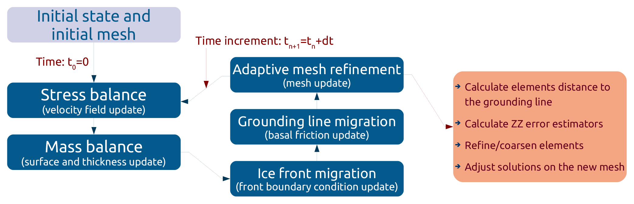
The solution sequence for transient ISSM simulations with AMR is summarized in Fig. 3. Details of AMR processes are itemized in Algorithm 11. In Fig. 3, the AMR is the last step to be executed for a given time step. This is an explicit approach, where a new adapted mesh is built for a given solution. In Algorithm 1, all processes involved in performing the AMR in ISSM are executed in step “e”, the remeshing core. Step “e.1” executes the mesh adaptation (refinement or coarsening of elements) and the other steps (“e.2” to “e.5”) prepare the adapted mesh, data structures and solutions for the next simulation time step.
Algorithm 1Transient simulation with AMR.
- 1.
Set initial solution state and initial mesh.
- 2.
While , do
- a.
call stress balance core (diagnostic),
- b.
call thickness balance core (prognostic),
- c.
call ice front migration core (level set adjustment),
- d.
call grounding line migration core (hydrostatic adjustment) and
- e.
call remesh core (AMR);
- e.1.
call AMR core (refine/coarsen mesh, Bamg or NeoPZ, serial in CPU no. 0),
- e.2.
call mesh partitioning (over all CPUs, serial),
- e.3.
build new data structures (all CPUs, parallel),
- e.4.
interpolate solutions (all CPUs, parallel) and
- e.5.
call geometry adjustment core (all CPUs, parallel).
- e.1.
- f.
Time increment .
- a.
- 3.
Post processing.
Bamg and NeoPZ perform the AMR (step “e.1”, Algorithm 1) in serial, considering the entire mesh. In our implementation, only one partition (whose CPU rank is no. 0) keeps the Bamg or NeoPZ entire mesh and is responsible for executing the AMR process.
Our AMR implementation keeps the number of partitions constant during the entire simulation time. The number and distribution of elements into the partitions vary every time AMR is called, since the mesh partitioning process (step “e.2”, Algorithm 1) generates partitions with a similar number of elements. This process avoids memory imbalance among the CPUs and overheads during the solver phase (Larour et al., 2012).
Each time remeshing is performed, the solutions and all data fields are interpolated from the old mesh onto the new mesh. This step is executed in parallel, where each CPU interpolates the solutions just on its own partition (step “e.4”, Algorithm 1). The construction of new data structures and the adjustment of solutions (steps “e.3” and “e.5”, respectively, Algorithm 1) are also executed in parallel, as is the computation of the refinement criteria (see Sect. 2.4).
All MPI communications in the remesh core (step “e”, Algorithm 1) are minimized to avoid overheads when large models are run. In order to minimize MPI calls, we perform a single communication of a large array that includes all data structures. In the interpolation process, for example, all relevant fields are collected by CPU no. 0 in a single vector structure in such a way that only one MPI broadcast is called. This approach is based on the fact that, in general, it is more efficient to perform few large MPI messages instead of carrying out many smaller ones (Reinders and Jeffers, 2015).
2.4 Refinement criteria
Grounding line dynamics are implemented in ISSM through an implicit level set function, ϕgl, based on a hydrostatic floatation criterion (Seroussi et al., 2014a):
where H is the ice thickness and is the flotation height, with ρi the ice density, ρw the ocean density and b the bedrock elevation (negative if below sea level). Figure 1 illustrates the GL position in a vertical cross-section of a marine ice sheet. The position of the GL is defined as
The performance of AMR depends on the refinement criterion (Devloo et al., 1987). We implement the three following criteria:
- a.
element distance to the GL, Rgl;
- b.
ZZ error estimator for deviatoric stress tensor, τ, and ice thickness, H; and
- c.
different combinations of (a) and (b).
Criterion (a) is based on a heuristic approach commonly applied (Cornford et al., 2013; Goldberg et al., 2009; Gudmundsson et al., 2012). The second criterion, (b), is based on the fact that high changes in the gradients in the velocity field (therefore, in the deviatoric stress tensor, τ) and ice thickness, H, are expected to be present near the grounding line. Criterion (c) extends and merges the features of the other two previous criteria. We define the AMR criterion used based on binary flags θ (=0 or 1) such that
We propose Algorithm 2, inspired by Devloo et al. (1987), to execute the refinement and coarsening processes under different criteria (AMR core, step “e.1” in Algorithm 1). The first three steps in Algorithm 2 compute the criterion according to the binary flags, θ, defined above. These steps are performed in parallel. Step “4” verifies, for each element in the mesh, if it should be refined; its distance to the GL and its ZZ errors are compared with prescribed limits (thresholds). The element is refined if at least one of the thresholds is exceeded, so long as its level of refinement is less than the maximum level chosen. This logical operation is performed by the operator “or” in the statement “if” in step “4”. Once an element is refined, it is identified as a group. Step “5” verifies for each group if it should be coarsened. To be coarsened, a group should meet all thresholds; the logical operator used in this case is “and” (statement “if” in step “5”). Algorithm 2 has two sets of thresholds (shown with max), for elements and for groups of elements. For the algorithm to work properly, these sets of thresholds should be different, following Devloo et al. (1987).
Algorithm 2AMR core: refinement criteria calculation, refinement and coarsening processes. e= element; g= group of elements that are nested and derived from a refined element; L(e)= level of refinement of the element e; maximum level of refinement; maximum threshold for element/group distance to the grounding line; maximum threshold for element/group error estimator (thickness/deviatoric stress); θ= binary flags that define the criteria.
- 1.
If θgl=1, then compute the element and group distances to the grounding line, Rgl(e) and Rgl(g).
- 2.
If θτ=1, then compute the element and group deviatoric stress error estimators, ϵτ(e) and ϵτ(g).
- 3.
If θH=1, then compute the element and group thickness error estimators, ϵH(e) and ϵH(g).
- 4.
For each element e such that , do
if or if or if ,
then refine e. - 5.
For each group g, do
if and if and if ,
then coarsen g.
2.5 ZZ error estimator
The generic form of the ZZ (Zienkiewicz and Zhu, 1987) error estimator ϵ(e) for a given element e is
where Ωe is the domain of the element e, ∇u is the gradient of the finite element solution u, and ∇u* is the smoothed reconstructed gradient, calculated on the element e as
and
where ψi is the ith P1 Lagrange shape function on element e, s is the number of shape functions of the element e (here, s=3), j is the jth element connected to the vertex i, k is the number of elements connected to vertex i, wj is the weight relative to the element j, and Wi is the sum of all weights for the vertex i. Here, the weights w are defined as the geometric area of the triangular elements. We implement the ZZ error estimator for the deviatoric stress tensor (τ), written in a vectorized form; i.e., for SSA we have . We also extend the estimator for the ice thickness (u=H). The ZZ estimator was conceived by Zienkiewicz and Zhu (1987) for linear elasticity, which involves elliptic equations. Applying the ZZ error estimator to the deviatoric stress tensor is therefore a natural extension, since the SSA equations are also elliptic. The ZZ estimator for the ice thickness highlights the regions of sharp bedrock gradient and could be used to improve the resolution of the bedrock geometry (e.g., see Fig. 8). See Sect. 2.4 and Algorithm 2 for an explanation of how these error estimates are combined.
We run two different benchmark experiments to evaluate the adaptive mesh refinement capabilities based on the MISMIP3D (Pattyn et al., 2013) and MISMIP+ (Asay-Davis et al., 2016) experiments. The following subsections briefly describe each setup. More details can be found in the respective references. All experiments are performed using the vertically integrated SSA equations (MacAyeal, 1989; Morland, 1987).
3.1 MISMIP3d setup
The MISMIP3d domain setup is rectangular and extends from 0 to 800 km in the x direction and from 0 to 50 km in the y direction. The bed elevation (b) varies only in the x direction, as follows:
Boundary conditions are applied as follows: a symmetric condition at x=0 so that ice velocity is equal to zero, a symmetric condition at y=0 (which represents the centerline of the ice stream) and a free-slip condition at y=50 km so that the flux through these surfaces is zero. Water pressure is applied at the ice front at x=800 km.
The ice viscosity, μ, is considered to be isotropic and to follow Glen's flow law (Cuffey and Paterson, 2010):
where B ( using Glen's rate factor A) is the ice viscosity parameter, is the effective strain rate, and n=3, a commonly used value for the exponent in Glen's flow law. The ice viscosity parameter, B, is uniform and constant over the domain and the time, and its value is equal to 2.15×10⁸ Pa s1∕3. A non-linear friction (Weertman) law is applied on grounded ice:
where τb is the basal shear stress, ub is the basal sliding velocity, C is the friction coefficient, and is the sliding law exponent. The basal friction coefficient, C, is also spatially uniform for all grounded ice and equal to 107 Pa m s1∕3.
The experiments are run starting from an initial configuration with a thin layer (100 m) of ice and with a constant accumulation rate of 0.5 m yr−1 applied over the whole domain. The experiments run forward in time until a steady-state condition is reached, which occurs after about 30 000 years. We compare the GL positions from different meshes at t=30 000 years.
We investigate the sensitivity of the AMR for which the refinement method is based on the element distance to the GL, Rgl (criterion a, Sect. 2.4). For comparison analysis, three different distances are used for the highest refinement level: Rgl=5, 10 and 15 km. These different meshes are labeled as R5, R10 and R15, respectively. The distance Rgl refers to the region with the highest level of refinement. For example, R5 means that 5 km on both sides of the GL (upstream and downstream) are refined with the highest level. Table 1 summarizes the criteria used for all experiments. The coarse mesh, that has a resolution of 5 km, is used as an initial mesh2 for all simulations and mesh generators (Bamg and NeoPZ). To analyze the convergence, we refine the coarse mesh 1 ×, 2 × and 3 ×. These three levels of refinement are applied to both uniform and adaptive meshes, and correspond to elements with 2.5, 1.25 and 0.63 km resolution, respectively. Table 2 presents the correspondence between refinement level and model resolution at the GL used in the experiments.
Table 1Refinement criteria for the adaptive mesh refinement (AMR) simulations.

“GL” is the grounding line. “τ” is the deviatoric stress tensor. The “distance to the GL” refers to the region with the highest level of refinement. For example, “AMR R5” means that 5 km on both sides of the GL (upstream and downstream) are refined with the highest level.
We also investigate the sensitivity of the AMR to GL parameterization into the elements (Seroussi et al., 2014a). Three sub-element parameterizations are tested: no sub-element parameterization (NSEP), sub-element parameterization 1 (SEP1) and sub-element parameterization 2 (SEP2). In the NSEP method, each element of the mesh is either grounded or floating, and the grounding line position is defined as the last grounded point. In the SEP1 and SEP2 methods, the grounding line position is located anywhere within an element and defined by the implicit level set function, ϕgl, which is based on the floating condition (see Sect. 2.4). The difference between SEP1 and SEP2 is how each one of these methods computes the basal friction to match the amount of grounded ice in the element. In the SEP1 approach, the basal friction coefficient (C) is reduced as , where Cg is the new basal friction coefficient for the element partially grounded, Ag is the area of grounded ice of this element, and A is the total area of the element. In the SEP2 technique, the basal friction is integrated (in the sense of the finite element method) only on the part where the element is grounded. This is done by changing the integration area from the original element to the grounded part of the element. We refer to Seroussi et al. (2014a) for a complete description of these sub-element parameterizations.
Table 2Levels of refinement tested in the experiments.

“CM” indicates coarse mesh, common for Bamg and NeoPZ.
3.2 MISMIP+ setup
The MISMIP+ domain is also rectangular, and its dimensions are km and km. The bed elevation is defined as follows:
with
and
where m, m, m, b4=343.91 m, m, km, d=500 m, Ly=80 km, wc=24 km, and fc=4 km. Figure 4 shows the bed elevation calculated with Eqs. (10), (11) and (12).

The ice is isothermal and the ice viscosity parameter, B, is equal to 1.1642×10⁸ Pa s1∕3 (uniform and constant over the domain and the time). The boundary conditions are similar to MISMIP3d. The friction model used here is a power law, Eq. (9), with a coefficient, C, equal to 3.160×10⁶ Pa m s1∕3 (spatially uniform for all grounded ice) and sliding law exponent, m, equal to 1∕3.
We run the experiments starting from an initial configuration with a 100 m thick layer of ice and run the simulations until a steady-state condition is reached (after 20 000 years). A constant accumulation rate of 0.3 m yr−1 is applied over the entire domain. The GL positions are compared at t=20 000 years.
To investigate further the sensitivity of the GL position to the refinement distance, Rgl, we choose distances with the highest refinement level equal to Rgl=5, 15 and 30 km, with meshes labeled as R5, R15 and R30, respectively (see Table 1). As for the MISMIP3d simulations, these distances refer to the region around the GL with the highest level of refinement. The same coarse mesh3 with a resolution of 4 km is used for Bamg and NeoPZ, and it is refined up to four times for both adaptive and uniform refinement approaches. The respective resolutions for the four refinement levels are 2, 1, 0.5 and 0.25 km. Table 2 summarizes the levels and the respective resolutions at the GL. All the MISMIP+ simulations are performed with sub-element parameterization type I, SEP1 (Seroussi et al., 2014a).
It is important to emphasize that the MISMIP+ bed elevation (Fig. 4) is calculated directly in the code every time AMR is called (step “e.5”, Algorithm 1). This procedure avoids excessive smoothing of the complex bedrock topography in the refined region.
For a given problem, the results from an AMR mesh should be as close as possible (within an acceptable tolerance) to those obtained with a uniformly refined mesh, for the same level of refinement (element resolution) in both meshes. This comparison is an indicator of the AMR performance to that given problem. Since Bamg and NeoPZ adapt the mesh in different ways, it is important to analyze how their differences impact the numerical solutions. Therefore, we first compare the results from the adaptive and uniform meshes using both Bamg and NeoPZ for the MISMIP3d and MISMIP+ experiments, and then we assess the time performance of the AMR in comparison with the uniformly refined mesh.
4.1 GL position comparison
4.1.1 MISMIP3d setup
Figure 5 presents the GL positions and the ice volume above floatation (VAF4) for different AMR meshes and sub-element parameterizations as a function of element resolutions. The refinement criterion used is the element distance to the GL, Rgl (see Table 1 and Sect. 2.4). GL positions and VAF obtained with uniformly refined meshes are also shown in Fig. 5. For NSEP, GL position varies between 200 and 520 km for meshes L0 (coarse mesh) and L3 (level of refinement equal to 3), respectively. For these same meshes, GL position varies between 620 and 600 km for SEP1 and between 550 and 600 km for SEP2.
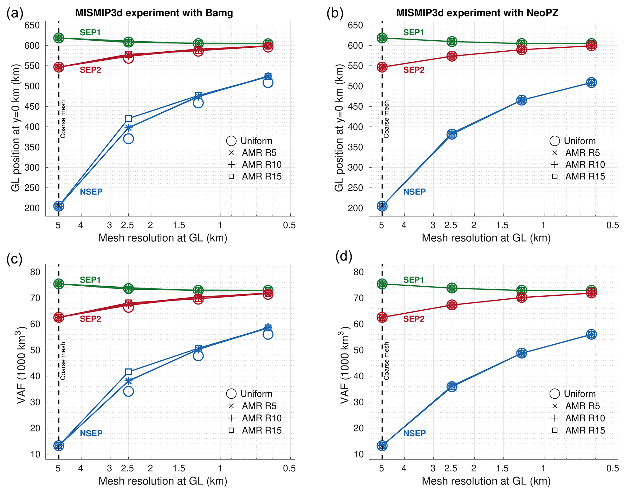
Figure 5GL positions (a, b) and VAF (c, d) at steady state obtained from the coarse mesh and from AMR using the refinement criterion based on the element distance to the GL, Rgl. Three element distances are used and compared: Rgl of 5, 10 and 15 km. The meshes generated with these distances are labeled as AMR R5, AMR R10 and AMR R15, respectively (see Tables 1 and 2). Results from uniformly refined meshes (labeled as uniform) are also shown. The simulations are carried out through the mesh generators Bamg (a, c) and NeoPZ (b, d) using three sub-element parameterizations: NSEP, SEP1 and SEP2.
We note that AMR meshes with NeoPZ produce GL positions that are very similar to the ones produced with uniformly refined mesh. This holds for all sub-element parameterizations. AMR with Bamg is more sensitive to NSEP, for which GL positions depend on the element distance to the GL (Rgl) used, especially for the lower refinement level (level equal to 1). Despite this, GL positions from AMR with Bamg are in agreement with uniformly refined meshes for SEP1 and SEP2. Similar behavior is observed in the VAF amounts.
4.1.2 MISMIP+ setup
The MISMIP+ bed topography (see Sect. 3.2 and Fig. 4) is designed to introduce a strong buttressing on the ice stream from the confined ice shelf. It is therefore expected that the results are more sensitive to the mesh refinement compared to simpler bedrock descriptions (e.g., MISMIP3d), since refining the mesh also improves the resolution of the bedrock geometry (see Sect. 3.2).
Figure 6 presents the coarse mesh and three examples of adaptive meshes obtained with Bamg and NeoPZ and different criteria: element distance to the GL, Rgl (equivalent to 5 km, R5) and error estimator ZZ (see Table 1). The figure also shows the GL positions obtained with these meshes and with the most refined uniform mesh (250 m resolution). Figure 6 provides an example of a case for which the GL position remains resolution dependent and refinement criterion dependent. We can note that, using the same criterion based on the element distance to the GL (mesh R5), Bamg and NeoPZ produce different meshes, as expected. For Bamg, the mesh transition zone between the lowest and highest resolutions is smoother than NeoPZ's mesh, since the resolutions in NeoPZ are obtained stepwise by nested elements. In Fig. 6, at the center of the domain (y=40 km), the GL position differs by 12 and 13 km between the most refined uniform mesh and the adaptive meshes generated by Bamg and NeoPZ, respectively. Between the coarse mesh and the adaptive meshes, the GL position differs by about 10 km (for both Bamg and NeoPZ). When the ZZ criterion is used, the GL positions differ by 6 km (17 km) in comparison with the one obtained from the most refined uniform mesh (coarse mesh).
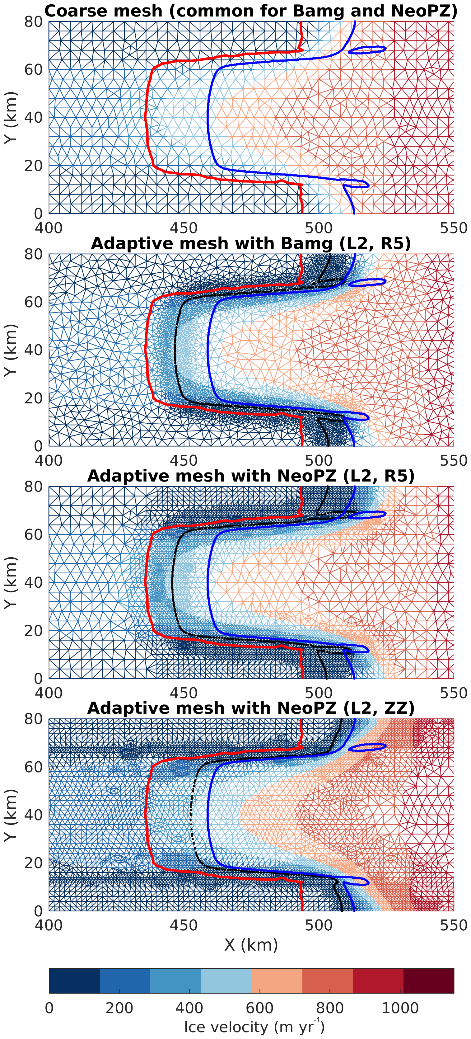
Figure 6Examples of adaptive meshes for the MISMIP+ experiment using different refinement criteria and mesh generators (see Tables 1 and 2). Red line: grounding line position at steady state obtained with the coarse mesh. Black dots: grounding line position at steady state obtained with each adaptive mesh. Blue line: grounding line position at steady state obtained with the most refined mesh (L4, uniform). The thresholds used in the ZZ criterion are described in the legend of Fig. 7.
Figure 7 presents a set of results for the grounding line position and the ice volume above floatation as a function of mesh resolution. AMR mesh dependency is clear in Fig. 7. For AMR with NeoPZ, GL positions obtained with AMR R5 differ from the ones produced by AMR R15 and AMR R30. Virtually AMR R15 and AMR R30 produce the same GL positions. For AMR with Bamg, AMR R5 and AMR R15 do not improve the position of the GL as the resolution increases. We can note the differences of GL positions from AMR (with both Bamg and NeoPZ) and from uniformly refined meshes are higher in comparison to the MISMIP3d experiment. The same AMR mesh dependency is observed in the VAF values.
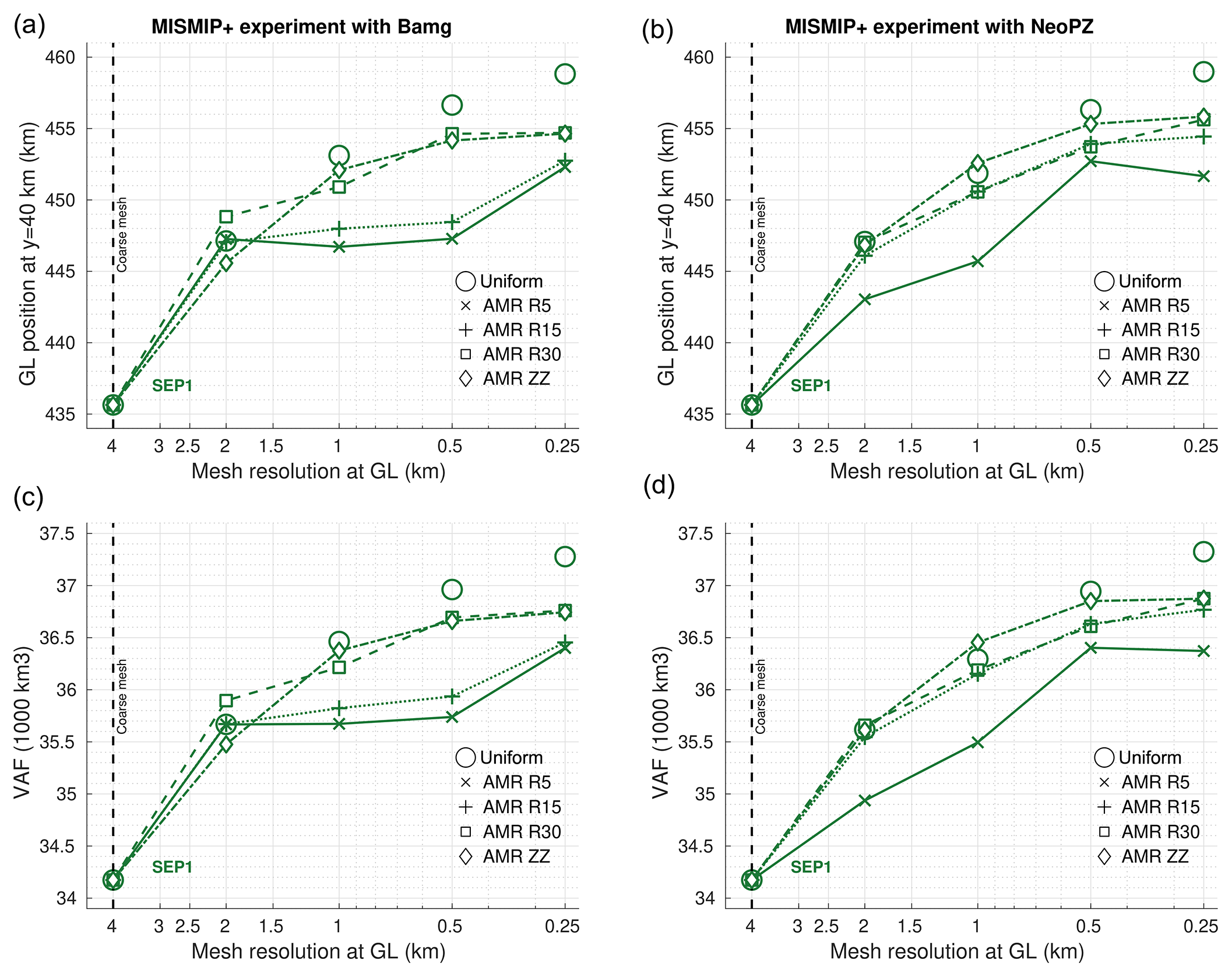
Figure 7GL positions (a, b) and VAF (c, d) obtained from the coarse mesh and from AMR for four refinement criteria: R5, R15, R30 and ZZ (see Tables 1 and 2). Results from uniformly refined meshes (uniform) are also shown. The simulations are carried out through the mesh generators Bamg (a, c) and NeoPZ (b, d) using sub-element parameterization 1 (SEP1). The thresholds for element/group used in the ZZ criterion are, respectively, (for both Bamg and NeoPZ) and for NeoPZ and for Bamg, where is the maximum error value observed in the coarse mesh.
To investigate the possible causes of this AMR mesh dependency, we perform the AMR using the ZZ error estimator calculated for the deviatoric stress tensor, τ (Table 1). The GL positions obtained with AMR ZZ are presented in Fig. 7. We observe that GL positions with AMR ZZ are closer to the ones obtained with uniform meshes, for all mesh resolutions. To understand this AMR ZZ result, we plot the spatial distributions of the ZZ error estimator for the coarse and adaptive meshes (using NeoPZ), as illustrated in Fig. 8 (see also the movies in the Supplement). The ZZ error values are normalized between 0 and 1. For the coarse mesh, we see in Fig. 8 that the error estimators calculated for the deviatoric stress tensor and the ice thickness present high values around the GL. In particular, for the ice thickness, the estimator also presents high values in the grounded part of the marine ice sheet, following the high gradient in the side walls of the bed topography (see Fig. 4). For AMR R5 meshes, there are high ZZ error values around the refined region. This is not observed when the refinement criterion used is the ZZ estimator (AMR ZZ; see Table 1), as expected. Using the ZZ criterion induces an equalization in the spatial distribution of the estimated errors, improving the solutions (e.g., GL position; see Fig. 7). In terms of efficiency, AMR ZZ generates fewer elements than AMR R30. At the end of the experiment and for a level of refinement equal to 4 (resolution equal to 250 m), using NeoPZ, AMR R30 mesh has 464 712 elements, while AMR ZZ mesh has 24 428 elements (i.e., only ∼5 % of the number of elements in AMR R30).
4.2 AMR time performance
To analyze the AMR performance in terms of computational time, we run the Ice1r experiment of MISMIP+ (Asay-Davis et al., 2016). The experiment starts from the steady-state condition and runs forward in time for 100 years with a basal melt rate applied. The time step is equal to 0.2 years (computed to fulfil the Courant–Friedrichs–Lewy, CFL, condition for the highest-resolution mesh). The non-linear SSA equations are solved using the Picard scheme and the Multifrontal Massively Parallel sparse direct Solver (Amestoy et al., 2001, 2006).
The purpose of the experiments described here is to assess the computational overhead when AMR is active. We initialize all the models using the steady-state solution obtained with the same AMR mesh (level of refinement and criteria) used to carry out the Ice1r experiment. This procedure emulates a common modeling practice (Cornford et al., 2013; Lee et al., 2015): the initial conditions are self-consistent with the AMR mesh, avoiding numerical artifacts during the transient simulation. All the experiments are run in parallel (16 cores) in a 2× Intel Xeon E5-2630 v3 2.40 GHz with 64 GB of RAM.
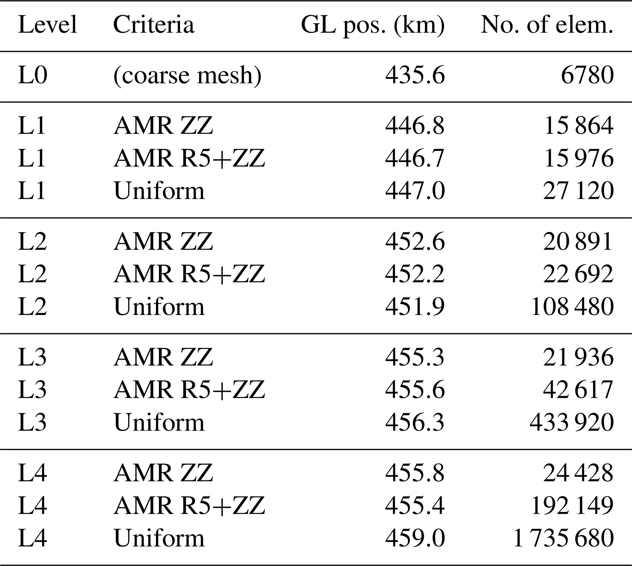
Table 3 presents GL positions obtained with different meshes at the end of experiment Ice1r, and the computational time and number of elements required for each mesh, as well as the criterion used. The levels of refinement are labeled as “L no.”; e.g., L3 means level 3 (see Table 2). Considering the GL position obtained from the highest-resolution mesh (L4 uniform) as a reference result, we compare the computational cost using uniform and AMR meshes to obtain the same result within a deviation of 1.5 %. In Table 3, only L3 uniform, L3 AMR R30, L3 AMR ZZ and L3 AMR R5+ZZ meshes produce this required accuracy. AMR R30 mesh has at least 25 % of the number of elements of the L3 uniform mesh, which represents virtually 80 % of the computational time using the uniform mesh. In terms of refinement criteria, AMR ZZ generates 20 % of the number of elements in comparison to AMR R30, which means virtually 25 % of computational time. Comparing AMR ZZ and L3 uniform, the computational time using the adaptive mesh represents at least 25 % of the computational time using the uniform mesh. The performance of Bamg and NeoPZ is similar, and the ratio of computational time and number of elements is virtually equal for both packages (not shown here).
Table 3AMR time performance comparison for the Ice1r experiment, MISMIP+.
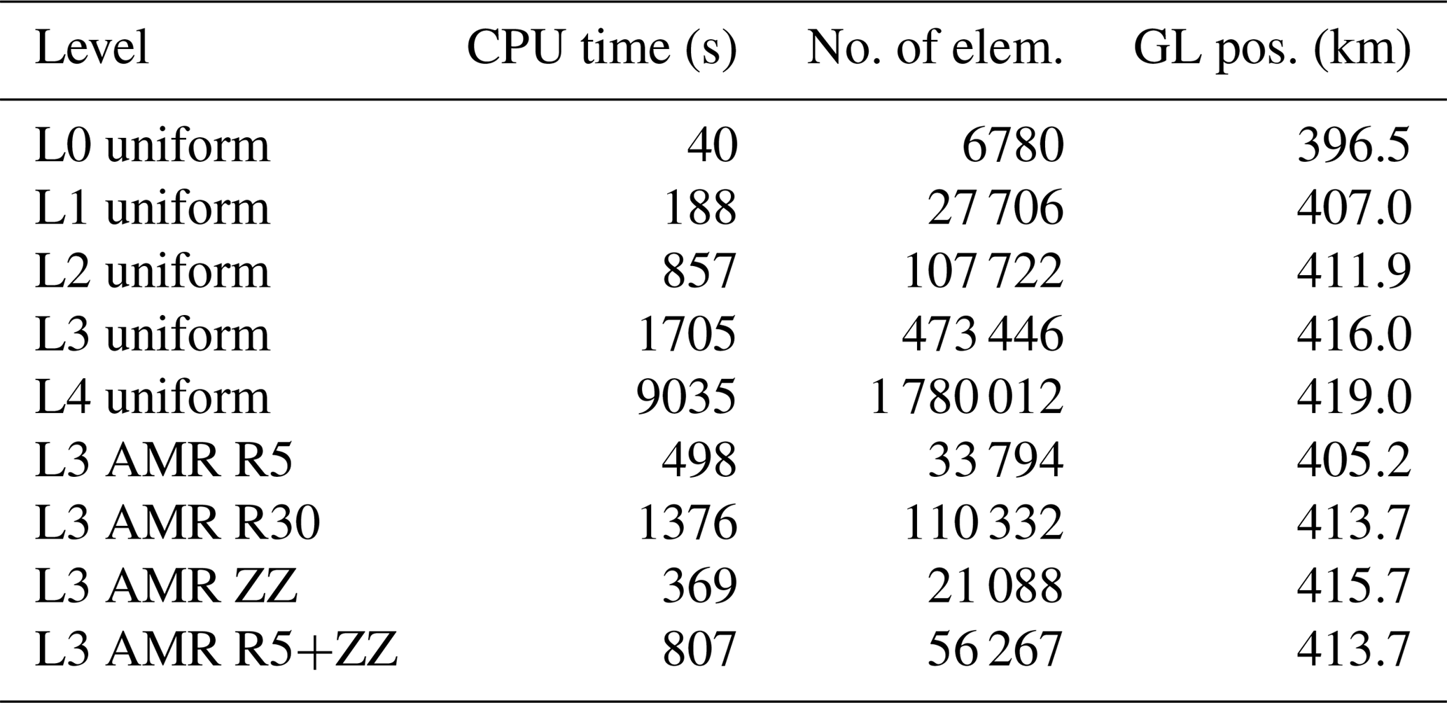
“Level” is the level of refinement. “No. of elem.” is the number of elements. “GL pos.” is the grounding line position at the end of the Ice1r experiment, MISMIP+. “AMR R5+ZZ” is the combination of the criteria ZZ error estimator (deviatoric stress tensor) and element distance to the GL (Rgl=5 km, R5). Mesher used: Bamg. The thresholds for element/group used in the ZZ criterion are, respectively, and for AMR ZZ, and and for AMR R5+ZZ, where is the maximum error value observed in the coarse mesh.
Figure 9 shows the element counts and the solution time for the AMR meshes normalized against the values for the equivalent uniform meshes. In Fig. 9, the solution time curve represents the relative savings due to AMR, while the gap between the two curves (solution time minus element counts) illustrates the overhead due to the AMR procedure. We note the AMR overhead decreases with the level of refinement and becomes reasonable for level 2 or higher.
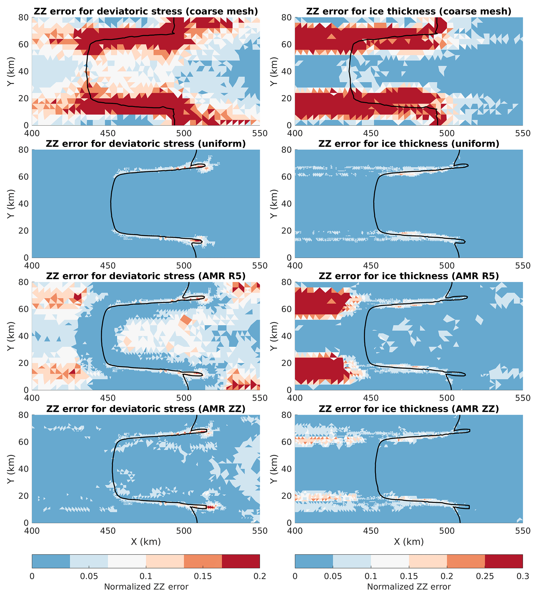
Figure 8Spatial distribution of the ZZ error estimator in the coarse and refined meshes (uniform and AMR) used in the MISMIP+ experiments. The ZZ error values are normalized between 0 and 1 using the maximum error value observed in the coarse mesh. Black lines are the grounding line positions at steady state obtained with the respective meshes. The refined meshes (uniform and AMR) are generated by NeoPZ considering the level of refinement equal to 2 (L2; see Table 2), and the criteria used (R5 and ZZ) are summarized in Table 1. The thresholds used in the AMR ZZ are described in the legend of Fig. 7.
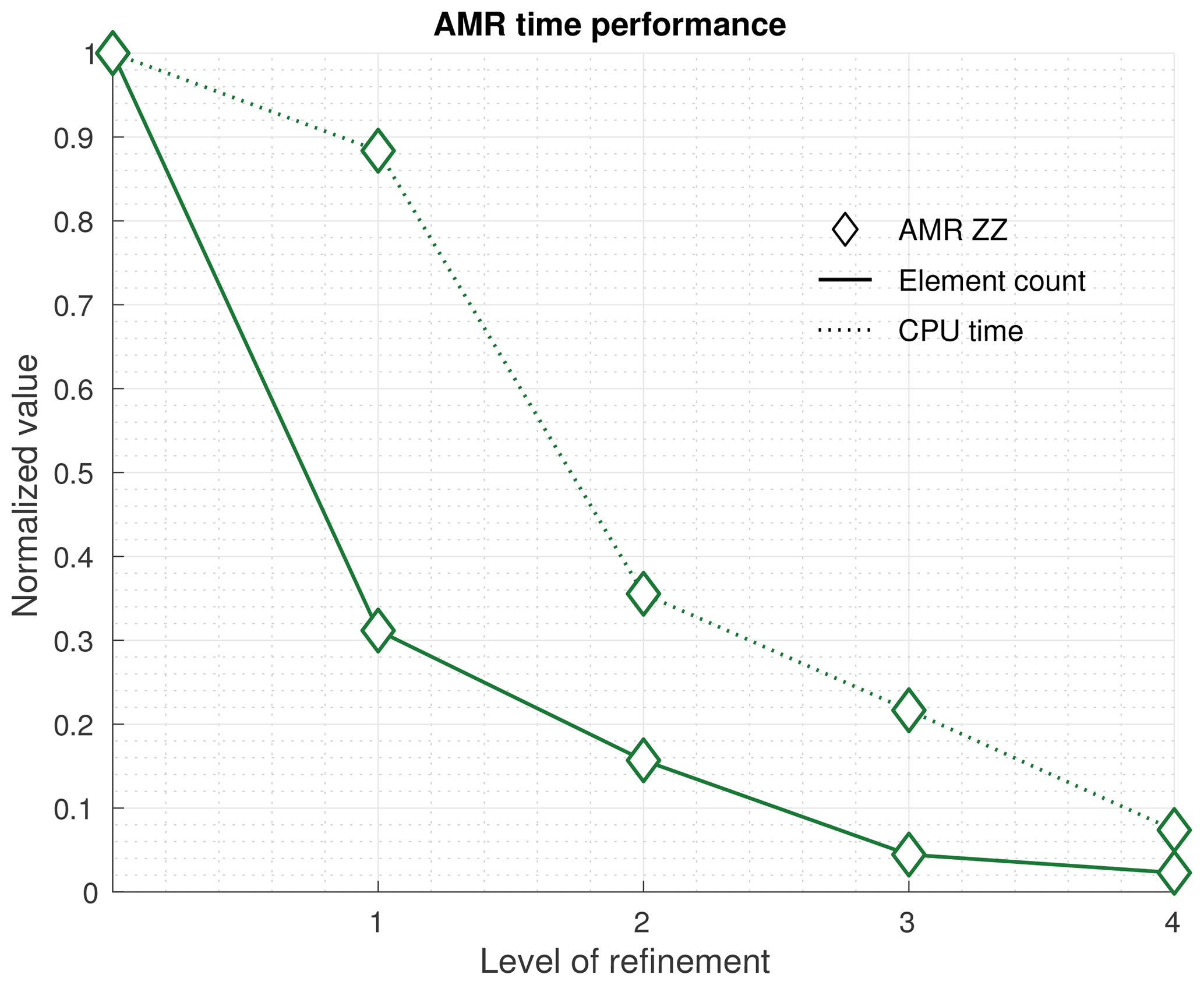
Figure 9Number of elements and CPU time for AMR meshes using the ZZ error estimator (AMR ZZ). The number of elements and CPU time are normalized by the respective values of the uniformly refined meshes. The normalized CPU time curve represents the AMR savings, while the difference between the two curves represents the adaptive mesh procedure cost. Mesher used: Bamg. The thresholds for element/group used in the AMR ZZ are, respectively, and for L1, and for L2, and for L3, and for L4, where is the maximum error value observed in the coarse mesh.
In this work, we describe the implementation of an adaptive mesh refinement approach in the Ice Sheet System Model (ISSM v4.14) as well as the performance of our implementation in terms of accuracy of the simulated grounding line position and simulation time. We investigate the adaptive meshes performance using a heuristic criterion based on the distance to the GL (Cornford et al., 2013; Durand et al., 2009; Goldberg et al., 2009; Gudmundsson et al., 2012), and we compare with an error estimator (Zienkiewicz and Zhu, 1987) based on the a posteriori analysis of the transient solutions (Cornford et al., 2013; Goldberg et al., 2009; Gudmundsson et al., 2012).
We rely on two different mesh generators, Bamg (Hecht, 2006) and NeoPZ (Devloo, 1997), that have different properties. It is therefore expected that their solutions are not identical. This explains the difference observed in the GL positions (and VAF) compared to uniform meshes for the three sub-element parameterizations (e.g., the MISMIP3d setup; Fig. 5).
NeoPZ generates nested meshes, which reduces errors in the interpolation step and is useful to assess AMR performance in comparison to uniformly refined mesh. Bamg's algorithm works differently: the fact that some vertices' positions change produces at least two side effects: (1) induced errors in the interpolation process; (2) positive or negative impact on the convergence of the solutions. The weight of the first side effect can be reduced using higher element distance to the GL (Rgl), for which the highest resolution is applied, and increasing the length of the mesh transition zone between fine and coarse elements. Higher-order interpolative schemes can be also used, as pointed out by Goldberg et al. (2009), to avoid solution diffusion. In ISSM, the interpolation scheme is carried out by P0 and P1 Lagrange polynomials, and we suspect these are enough for our AMR procedure. The weight of the second side effect depends on the problem considered. We suspect that for GL dynamics this effect has overall a positive impact, once updating vertex positions is somewhat similar to the moving mesh technique, although the GL is not explicitly defined in our approach as in other studies (Vieli and Payne, 2005). This argument is based on the results shown here, for both MISMIP3d and MISMIP+ setups. Some mesh packages and finite element libraries related to NeoPZ are Deal II (Bangerth et al., 2007), Hermes (Šolín et al., 2008), libMesh (Kirk et al., 2006) and HP90 (Demkowicz et al., 1998). Mesh generators related to Bamg are MMG (Dapogny et al., 2014), Yams (Frey, 2001) and Gmsh (Geuzaine and Remacle, 2009). So, we expect that the results shown in this work would be reproduced with these related packages.
The results from MISMIP3d suggest that, independently of the sub-element parameterization and refinement level, refining elements within a 5 km region with highest resolution around the GL is enough to generate solutions similar to the ones produced by uniform meshes. This holds for Bamg and NeoPZ (Fig. 5). Cornford et al. (2013) presented similar results for MISMIP3d using SSA equations through BISICLES, an AMR finite-volume-based ice sheet model. Based on the MISMIP3d experiment, they concluded that refining four cells on either side of the GL was enough to achieve results similar to uniform meshes for all levels of refinement.
For MISMIP+, a minimal distance of 30 km for the highest resolution around the GL is necessary to accurately capture the GL position (Fig. 7). Nevertheless, there is a residual between GL positions from AMR and uniform meshes. This AMR mesh dependency can be explained by the bed topography of MISMIP+ (Fig. 4); the high gradient in the side walls induces numerical errors on the gradients of the velocity field (deviatoric stress tensor, near the GL) and ice thickness (on grounded ice), as illustrated by the spatial distribution of the a posteriori error estimator used here (Fig. 8). For the MISMIP3d setup, the highest values of the error estimate concentrate only around the GL (not shown here), which explains why a few kilometers of high resolution near the GL improve the GL positions.
Figures 5 and 7 present a picture of the impact of mesh resolution in integrated quantities like VAF. The VAF curves follow the GL position behavior, presenting the same AMR mesh dependency in the MISMIP+ setup. Therefore, the accuracy of VAF depends on the accuracy of the GL dynamics. Since VAF changes represent potential sea level rise, we highlight that the GL movement should be accurately tracked in ice sheet models.
Since numerical errors are not only concentrated near the GL for the MISMIP+ setup, an error estimator is likely more appropriate to understand the error structure of the problem, to guide the refinement and to reduce the error estimates along the domain, improving AMR performance. This explains why a simple test with the AMR ZZ produces better convergence with much fewer elements than AMR based on the heuristic criterion (element distance to the GL, Fig. 7). Related works have used proxies of error estimators: Goldberg et al. (2009) used the jumps in strain rate between adjacent cells; Gudmundsson et al. (2012) used the second derivative of the ice thickness; Cornford et al. (2013) used the Laplacian of the velocity field and Gillet-Chaulet et al. (2017) used the estimator proposed by Frey and Alauzet (2005), whose metric is based on a priori interpolation error calculated by the field's Hessian matrix (second derivative). The ZZ used here is a true a posteriori error estimator based on the recovered gradient (Ainsworth and Oden, 2000), widely used in the finite element community (Ainsworth et al., 1989; Grätsch and Bathe, 2005) and suitable to be implemented in ice sheet models, including those based on finite volumes or finite differences. As the MISMIP+ bed geometry is more realistic than MISMIP3d, we can expect similar results for real glaciers, i.e., high numerical errors present in regions not necessarily adjacent to the GL.
Further analysis with ZZ or another error estimator should be developed to improve the AMR criterion used in ice sheet modeling. An important issue to be investigated is the interpolation of real bed topography directly from a dataset every time AMR is carried out. This interpolation increases bed resolution according to mesh adaptation, which reduces the smoothness of the bed in the model (since real beds are not necessarily smooth). The reduction of the bed smoothness induces some numerical errors and counterbalances the effect of mesh adaptation, increasing AMR mesh dependency. Real bed topographies should be analyzed in benchmark models as well as in real ice sheet domains. Our current AMR implementation interpolates the bed elevation from the coarse mesh, except for the MISMIP+ experiment, for which we hard-coded the calculation of the bed topography directly in the code (in this case, AMR reduces the smoothness of the bed in the model, but as there is no small-scale bed topography, the numerical error based on the ZZ error estimator for the ice thickness is reduced). The interpolation from a dataset will be implemented in ISSM in the future. Based on this discussion and the results shown in this study, we recommend AMR with the combination of the heuristic criterion (using a minimal distance, e.g., 5 km) with an associated error estimator. Our recommendation is based on the following: we know a priori that applying high resolution around the GL would reduce the error caused by the basal friction discretization within the elements. In fact, applying only an error estimator does not guarantee that the elements around the GL are refined until the highest (desired) resolution. We noted this for the MISMIP+ setup (see the last mesh in Fig. 6). On the other hand, only imposing fine mesh resolution near the GL does not ensure that the GL position is correctly captured because the extension of the grounding zone (Schoof, 2007b) depends on the physical parameters of the ice sheet. Interestingly, for the MISMIP+ setup, the combination of the heuristic criterion with the ZZ error estimator (AMR R5+ZZ) and the AMR ZZ produce similar results (as shown in Table 4), which does not guarantee that it would be the case for real ice sheets. Therefore, for real ice sheets, we suspect that using both criteria (R5+ZZ) should work properly. Tests varying AMR parameters (distance to the GL, maximum thresholds for the error estimator, level of refinement, etc.) should be carried before any ice sheet simulation to optimize AMR performance in terms of both solutions and computational time.
Table 4AMR criteria comparison for the MISMIP+ experiment.
“Level” is the level of refinement. “`GL pos.” is the grounding line position at the end of the experiment. “No. of elem.” is the number of elements. “AMR R5+ZZ” is the combination of the criteria ZZ error estimator (deviatoric stress tensor) and element distance to the GL (Rgl of 5 km, R5). Mesher used: NeoPZ. The thresholds used in the ZZ criterion are described in the legend of Fig. 7.
The grounding zone is not the only place where AMR can be applied. Ice front and calving dynamics (Todd et al., 2018) as well as shear margins in ice streams (Haseloff et al., 2015) are examples for which adaptive meshes can improve numerical solutions with reduced computational efforts. In ISSM, the AMR can be applied to these regions through extension of Algorithm 2. Other experiments (not shown here) testing the AMR to refine the ice front region show promising results (Santos et al., 2018).
Our AMR performance analysis shows that the computational time in AMR simulations reaches up to 1 order of magnitude less in comparison to models based on uniform meshes. Computational time and solution accuracy of AMR depend on the physical problem and the refinement criterion used. In this work, even with hundreds of elements generated (e.g., meshes AMR R30), the computational time is satisfactory. This is observed for both NeoPZ and Bamg. Further analysis should be carried out to check the performance in real ice sheets and in higher computational scale (thousand of elements), but the results presented in this study suggest that our AMR implementation strategy is adapted to the modeling questions being investigated. Our AMR computation time compares to Cornford et al. (2013), in which AMR simulations spend approximately one-third of CPU time needed in simulations performed by uniform meshes.
We implemented dynamic AMR into ISSM and tested its performance on two different experiments with different refinement criteria. The comparison between Bamg and NeoPZ shows that they present similar performance, and the choice of which should be used is up to the user. Moreover, users using Bamg (or a similar mesh generator) should pay attention to the minimal extension of the mesh transition zone to reduce numerical errors (e.g., in the interpolation step). NeoPZ is more suitable with error estimators, as well as in AMR performance comparison. Based on the AMR mesh sensitivity observed here, we conclude that AMR without an error estimator should be avoided, mainly in setups where bedrock induces complex stress distributions and/or strong buttressing. In real bedrock topographies, where small-scale features may play an important role, an error estimator is suitable to guide the AMR. Further research should be carried out in order to evaluate AMR performance in real bed geometries. Our recommendation to improve the AMR performance while minimizing computational effort is the combination of the heuristic criteria, applying a minimal distance around the GL (e.g., 5 km), with an error estimator. The simple tests with the ZZ error estimator show a significant potential, mostly due to its simple implementation and performance. The AMR technique in ISSM can be extended to others physical processes such that the evolution of ice sheets and, consequently the sea level rise, can be accurately modeled and projected.
The adaptive mesh refinements are currently implemented in the ISSM code for triangular elements. The code can be download, compiled and executed following the instructions available on the ISSM website: https://issm.jpl.nasa.gov/download (last access: 4 January 2019, Larour et al., 2012).
The supplement related to this article is available online at: https://doi.org/10.5194/gmd-12-215-2019-supplement.
TDS and MM implemented the AMR in the ISSM. MM and PRBD guided the AMR implementation. HS and TDS designed the experimental setups. HS, MM and PRBD led the analysis of the results. TDS, PRBD and JCS led the initial writing of the paper. All authors contributed to writing the final version of the paper.
The authors declare that they have no conflict of interest.
This work was performed at the University of Campinas (UNICAMP) and Federal
University of Rio Grande do Sul (UFRGS) with financial support from CNPq –
Conselho Nacional de Desenvolvimento Científico e Tecnológico, Brazil,
PhD scholarship no. 140186/2015-8 – and at the University of California,
Irvine, under a contract with the National Aeronautics and Space
Administration (NASA) Cryospheric Sciences Program
(no. NNX14AN03G). Hélène Seroussi is funded by grants from the NASA Cryospheric Sciences Program.
Edited by: Alexander Robel
Reviewed by: Daniel
Martin and one anonymous referee
Ainsworth, M. and Oden, J. T.: A Posterori Error Estimation in Finite Element Analysis, Pure and Applied Mathematics: A Wiley Series of Texts, Monographs and Tracts, Wiley-Interscience, New York, NY, USA, 1st Edn., 2000. a
Ainsworth, M., Zhu, J. Z., Craig, A. W., and Zienkiewicz, O. C.: Analysis of the Zienkiewicz–Zhu a-posteriori error estimator in the finite element method, Int. J. Numer. Meth. Eng., 28, 2161–2174, https://doi.org/10.1002/nme.1620280912, 1989. a
Amestoy, P. R., Duff, I. S., L'Excellent, J.-Y., and Koster, J.: A Fully Asynchronous Multifrontal Solver Using Distributed Dynamic Scheduling, SIAM J. Matrix Anal. A., 23, 15–41, https://doi.org/10.1137/S0895479899358194, 2001. a
Amestoy, P. R., Guermouche, A., L'Excellent, J.-Y., and Pralet, S.: Hybrid scheduling for the parallel solution of linear systems, Parallel Comput., 32, 136–156, https://doi.org/10.1016/j.parco.2005.07.004, 2006. a
Anderson, D. A., Tannehill, J. C., and Pletcher, R. H.: Computational Fluid Mechanics and Heat Transfer, Series in computational methods in mechanics and thermal sciences, McGraw-Hill Book Company, USA, 1984. a
Asay-Davis, X. S., Cornford, S. L., Durand, G., Galton-Fenzi, B. K., Gladstone, R. M., Gudmundsson, G. H., Hattermann, T., Holland, D. M., Holland, D., Holland, P. R., Martin, D. F., Mathiot, P., Pattyn, F., and Seroussi, H.: Experimental design for three interrelated marine ice sheet and ocean model intercomparison projects: MISMIP v. 3 (MISMIP+), ISOMIP v. 2 (ISOMIP+) and MISOMIP v. 1 (MISOMIP1), Geosci. Model Dev., 9, 2471–2497, https://doi.org/10.5194/gmd-9-2471-2016, 2016. a, b, c, d, e
Bangerth, W., Hartmann, R., and Kanschat, G.: Deal.II – A General-purpose Object-oriented Finite Element Library, ACM T. Math. Software, 33, 24, https://doi.org/10.1145/1268776.1268779, 2007. a
Berger, M. and Colella, P.: Local adaptive mesh refinement for shock hydrodynamics, J. Comput. Phys., 82, 64–84, https://doi.org/10.1016/0021-9991(89)90035-1, 1989. a, b
Bindschadler, R. A., Nowicki, S., Abe-Ouchi, A., Aschwanden, A., Choi, H., Fastook, J., Granzow, G., Greve, R., Gutowski, G., Herzfeld, U., Jackson, C., Johnson, J., Khroulev, C., Levermann, A., Lipscomb, W. H., Martin, M. A., Morlighem, M., Parizek, B. R., Pollard, D., Price, S. F., Ren, D., Saito, F., Sato, T., Seddik, H., Seroussi, H., Takahashi, K., Walker, R., and Wang, W. L.: Ice-sheet model sensitivities to environmental forcing and their use in projecting future sea level (the SeaRISE project), J. Glaciol., 59, 195–224, https://doi.org/10.3189/2013JoG12J125, 2013. a
Calle, J. L. D., Devloo, P. R., and Gomes, S. M.: Implementation of continuous hp-adaptive finite element spaces without limitations on hanging sides and distribution of approximation orders, Comput. Math. Appl., 70, 1051–1069, https://doi.org/10.1016/j.camwa.2015.06.033, 2015. a, b
Christie, F. D. W., Bingham, R. G., Gourmelen, N., Tett, S. F. B., and Muto, A.: Four-decade record of pervasive grounding line retreat along the Bellingshausen margin of West Antarctica, Geophys. Res. Lett., 43, 5741–5749, https://doi.org/10.1002/2016GL068972, 2016. a
Church, J., Clark, P., Cazenave, A., Gregory, J., Jevrejeva, S., Levermann, A., Merrifield, M., Milne, G., Nerem, R., Nunn, P., Payne, A., Pfeffer, W., Stammer, D., and Unnikrishnan, A.: Sea Level Change, in: Climate Change 2013: The Physical Science Basis. Contribution of Working Group I to the Fifth Assessment Report of the Intergovernmental Panel on Climate Change, edited by: Stocker, T., Qin, D., Plattner, G.-K., Tignor, M., Allen, S., Boschung, J., Nauels, A., Xia, Y., Bex, V., and Midgley, P., 1137–1216, Cambridge University Press, Cambridge, UK and New York, NY, USA, 2013. a
Cornford, S. L., Martin, D. F., Graves, D. T., Ranken, D. F., Brocq, A. M. L., Gladstone, R. M., Payne, A. J., Ng, E. G., and Lipscomb, W. H.: Adaptive mesh, finite volume modeling of marine ice sheets, J. Comput. Phys., 232, 529–549, https://doi.org/10.1016/j.jcp.2012.08.037, 2013. a, b, c, d, e, f, g, h, i, j
Cuffey, K. and Paterson, W. S. B.: The Physics of Glaciers, 4th Edn., Elsevier, Oxford, 2010. a
Dapogny, C., Dobrzynski, C., and Frey, P.: Three-dimensional adaptive domain remeshing, implicit domain meshing, and applications to free and moving boundary problems, J. Comput. Phys., 262, 358–378, https://doi.org/10.1016/j.jcp.2014.01.005, 2014. a
DeConto, R. and Pollard, D.: Contribution of Antarctica to past and future sea-level rise, Nature, 531, 591–597, https://doi.org/10.1038/nature17145, 2016. a
Demkowicz, L., Gerdes, K., Schwab, C., Bajer, A., and Walsh, T.: HP90: A general and flexible Fortran 90 hp-FE code, Computing and Visualization in Science, 1, 145–163, https://doi.org/10.1007/s007910050014,1998. a
Devloo, P., Oden, J., and Strouboulis, T.: Implementation of an adaptive refinement technique for the SUPG algorithm, Comput. Method. Appl. M., 61, 339–358, https://doi.org/10.1016/0045-7825(87)90099-5,1987. a, b, c, d, e, f
Devloo, P. R. B.: PZ: An object oriented environment for scientific programming, Comput. Method. Appl. M., 150, 133–153, https://doi.org/10.1016/S0045-7825(97)00097-2, 1997. a, b, c
Durand, G., Gagliardini, O., Zwinger, T., Meur, E. L., and Hindmarsh, R. C.: Full Stokes modeling of marine ice sheets: influence of the grid size, Ann. Glaciol., 50, 109–114, https://doi.org/10.3189/172756409789624283, 2009. a, b
Dutrieux, P., De Rydt, J., Jenkins, A., Holland, P. R., Ha, H. K., Lee, S. H., Steig, E. J., Ding, Q., Abrahamsen, E. P., and Schröder, M.: Strong Sensitivity of Pine Island Ice-Shelf Melting to Climatic Variability, Science, 343, 174–178, https://doi.org/10.1126/science.1244341, 2014. a
Favier, L., Durand, G., Cornford, S. L., Gudmundsson, G. H., Gagliardini, O., Gillet-Chaulet, F., Zwinger, T., Payne, A. J., and Le Brocq, A. M.: Retreat of Pine Island Glacier controlled by marine ice-sheet instability, Nature Climate Change, 4, 117–121, https://doi.org/10.1038/nclimate2094, 2014. a
Feldmann, J., Albrecht, T., Khroulev, C., Pattyn, F., and Levermann, A.: Resolution-dependent performance of grounding line motion in a shallow model compared with a full-Stokes model according to the MISMIP3d intercomparison, J. Glaciol., 60, 353–360, https://doi.org/10.3189/2014JoG13J093, 2014. a
Fretwell, P., Pritchard, H. D., Vaughan, D. G., Bamber, J. L., Barrand, N. E., Bell, R., Bianchi, C., Bingham, R. G., Blankenship, D. D., Casassa, G., Catania, G., Callens, D., Conway, H., Cook, A. J., Corr, H. F. J., Damaske, D., Damm, V., Ferraccioli, F., Forsberg, R., Fujita, S., Gim, Y., Gogineni, P., Griggs, J. A., Hindmarsh, R. C. A., Holmlund, P., Holt, J. W., Jacobel, R. W., Jenkins, A., Jokat, W., Jordan, T., King, E. C., Kohler, J., Krabill, W., Riger-Kusk, M., Langley, K. A., Leitchenkov, G., Leuschen, C., Luyendyk, B. P., Matsuoka, K., Mouginot, J., Nitsche, F. O., Nogi, Y., Nost, O. A., Popov, S. V., Rignot, E., Rippin, D. M., Rivera, A., Roberts, J., Ross, N., Siegert, M. J., Smith, A. M., Steinhage, D., Studinger, M., Sun, B., Tinto, B. K., Welch, B. C., Wilson, D., Young, D. A., Xiangbin, C., and Zirizzotti, A.: Bedmap2: improved ice bed, surface and thickness datasets for Antarctica, The Cryosphere, 7, 375–393, https://doi.org/10.5194/tc-7-375-2013, 2013. a
Frey, P.: YAMS A fully Automatic Adaptive Isotropic Surface Remeshing Procedure, Tech. rep., INRIA, 2001. a
Frey, P. and Alauzet, F.: Anisotropic mesh adaptation for CFD computations, Comput. Meth. Appl. M., 194, 5068–5082, https://doi.org/10.1016/j.cma.2004.11.025, 2005. a
Gagliardini, O., Zwinger, T., Gillet-Chaulet, F., Durand, G., Favier, L., de Fleurian, B., Greve, R., Malinen, M., Martín, C., Råback, P., Ruokolainen, J., Sacchettini, M., Schäfer, M., Seddik, H., and Thies, J.: Capabilities and performance of Elmer/Ice, a new-generation ice sheet model, Geosci. Model Dev., 6, 1299–1318, https://doi.org/10.5194/gmd-6-1299-2013, 2013. a
Geuzaine, C. and Remacle, J.-F.: Gmsh: A 3-D finite element mesh generator with built-in pre- and post-processing facilities, Int. J. Numer. Meth. Eng., 79, 1309–1331, https://doi.org/10.1002/nme.2579, 2009. a
Gillet-Chaulet, F., Tavard, L., Merino, N., Peyaud, V., Brondex, J., Durand, G., and Gagliardini, O.: Anisotropic mesh adaptation for marine ice-sheet modelling, Geophys. Res. Abstr., EGU2017-2048, EGU General Assembly 2017, Vienna, Austria, 2017. a, b
Gladstone, R. M., Lee, V., Vieli, A., and Payne, A. J.: Grounding line migration in an adaptive mesh ice sheet model, J. Geophys. Res.-Earth, 115, F04014, https://doi.org/10.1029/2009JF001615, 2010. a, b
Goldberg, D., Holland, D. M., and Schoof, C.: Grounding line movement and ice shelf buttressing in marine ice sheets, J. Geophys. Res.-Earth, 114, F04026, https://doi.org/10.1029/2008JF001227, 2009. a, b, c, d, e, f, g
Grätsch, T. and Bathe, K.-J.: A posteriori error estimation techniques in practical finite element analysis, Comput. Struct., 83, 235–265, https://doi.org/10.1016/j.compstruc.2004.08.011, 2005. a
Gudmundsson, G. H., Krug, J., Durand, G., Favier, L., and Gagliardini, O.: The stability of grounding lines on retrograde slopes, The Cryosphere, 6, 1497–1505, https://doi.org/10.5194/tc-6-1497-2012, 2012. a, b, c, d, e, f
Haseloff, M., Schoof, C., and Gagliardini, O.: A boundary layer model for ice stream margins, J. Fluid Mech., 781, 353–387, https://doi.org/10.1017/jfm.2015.503, 2015. a
Hecht, F.: A few snags in mesh adaptation loops, in: Proceedings of the 14th International Meshing Roundtable, edited by: Hanks, B. W., 301–311, Springer-Verlag Berlin Heidelberg, Germany, 2005. a, b
Hecht, F.: BAMG: Bidimensional Anisotropic Mesh Generator, Tech. rep., FreeFem, 2006. a, b, c, d
Jacobs, S. S., Jenkins, A., Giulivi, C. F., and Dutrieux, P.: Stronger ocean circulation and increased melting under Pine Island Glacier ice shelf, Nat. Geosci., 4, 519–523, https://doi.org/10.1038/ngeo1188, 2011. a
Jevrejeva, S., Grinsted, A., and Moore, J. C.: Upper limit for sea level projections by 2100, Environ. Res. Lett., 9, 104008, https://doi.org/10.1088/1748-9326/9/10/104008, 2014. a
Jouvet, G. and Gräser, C.: An adaptive Newton multigrid method for a model of marine ice sheets, J. Comput. Phys., 252, 419–437, https://doi.org/10.1016/j.jcp.2013.06.032, 2013. a
Katz, R. F. and Worster, M. G.: Stability of ice-sheet grounding lines, P. Roy. Soc. Lond. A, 466, 1597–1620, https://doi.org/10.1098/rspa.2009.0434, 2010. a
Kimura, S., Jenkins, A., Dutrieux, P., Forryan, A., Naveira Garabato, A. C., and Firing, Y.: Ocean mixing beneath Pine Island Glacier ice shelf, West Antarctica, J. Geophys. Res.-Ocean, 121, 8496–8510, https://doi.org/10.1002/2016JC012149, 2016. a
Kirk, B. S., Peterson, J. W., Stogner, R. H., and Carey, G. F.: libMesh: a C library for parallel adaptive mesh refinement/coarsening simulations, Eng. Comput., 22, 237–254, https://doi.org/10.1007/s00366-006-0049-3, 2006. a
Larour, E., Seroussi, H., Morlighem, M., and Rignot, E.: Continental scale, high order, high spatial resolution, ice sheet modeling using the Ice Sheet System Model (ISSM), J. Geophys. Res.-Earth, 117, F01022, https://doi.org/10.1029/2011JF002140, 2012. a, b, c, d
Lee, V., Cornford, S. L., and Payne, A. J.: Initialization of an ice-sheet model for present-day Greenland, Ann. Glaciol., 56, 129–140, https://doi.org/10.3189/2015AoG70A121, 2015. a, b
Leguy, G. R., Asay-Davis, X. S., and Lipscomb, W. H.: Parameterization of basal friction near grounding lines in a one-dimensional ice sheet model, The Cryosphere, 8, 1239–1259, https://doi.org/10.5194/tc-8-1239-2014, 2014. a
MacAyeal, D.: Large-scale ice flow over a viscous basal sediment: Theory and application to ice stream B, Antarctica, J. Geophys. Res.-Sol. Ea., 94, 4071–4087, https://doi.org/10.1029/JB094iB04p04071, 1989. a, b
Mercer, J. H.: West Antarctic ice sheet and CO2 greenhouse effect: a threat of disaster, Nature, 271, 321–325, https://doi.org/10.1038/271321a0, 1978. a
Morland, L. W.: Unconfined ice shelf flow, in: Dynamics of the West Antarctic Ice Sheet, edited by: Van der Veen, C. and Oerlemans, J., Vol. 4 of Glaciology and Quaternary Geology, 99–116, Springer, Dordrecht, the Netherlands, 1987. a, b
Morlighem, M., Rignot, E., Seroussi, H., Larour, E., Ben Dhia, H., and Aubry, D.: Spatial patterns of basal drag inferred using control methods from a full-Stokes and simpler models for Pine Island Glacier, West Antarctica, Geophys. Res. Lett., 37, L14502, https://doi.org/10.1029/2010GL043853, 2010. a
Oden, J., Strouboulis, T., and Devloo, P.: Adaptive finite element methods for the analysis of inviscid compressible flow: Part I. Fast refinement/unrefinement and moving mesh methods for unstructured meshes, Comput. Meth. Appl. M., 59, 327–362, https://doi.org/10.1016/0045-7825(86)90004-6, 1986. a
Pattyn, F.: A new three-dimensional higher-order thermomechanical ice sheet model: Basic sensitivity, ice stream development, and ice flow across subglacial lakes, J. Geophys. Res., 108, 1–15, 2003. a
Pattyn, F.: Sea-level response to melting of Antarctic ice shelves on multi-centennial timescales with the fast Elementary Thermomechanical Ice Sheet model (f.ETISh v1.0), The Cryosphere, 11, 1851–1878, https://doi.org/10.5194/tc-11-1851-2017, 2017. a
Pattyn, F., Schoof, C., Perichon, L., Hindmarsh, R. C. A., Bueler, E., de Fleurian, B., Durand, G., Gagliardini, O., Gladstone, R., Goldberg, D., Gudmundsson, G. H., Huybrechts, P., Lee, V., Nick, F. M., Payne, A. J., Pollard, D., Rybak, O., Saito, F., and Vieli, A.: Results of the Marine Ice Sheet Model Intercomparison Project, MISMIP, The Cryosphere, 6, 573–588, https://doi.org/10.5194/tc-6-573-2012, 2012. a, b
Pattyn, F., Perichon, L., Durand, G., Favier, L., Gagliardini, O., Hindmarsh, R. C., Zwinger, T., Albrecht, T., Cornford, S., Docquier, D., Fürst, J. J., Goldberg, D., Gudmundsson, G. H., Humbert, A., Hütten, M., Huybrechts, P., Jouvet, G., Kleiner, T., Larour, E., Martin, D., Morlighem, M., Payne, A. J., Pollard, D., Rückamp, M., Rybak, O., Seroussi, H., Thoma, M., and Wilkens, N.: Grounding-line migration in plan-view marine ice-sheet models: results of the ice2sea MISMIP3d intercomparison, J. Glaciol., 59, 410–422, https://doi.org/10.3189/2013JoG12J129, 2013. a, b, c, d
Pollard, D. and DeConto, R. M.: Modelling West Antarctic ice sheet growth and collapse through the past five million years, Nature, 458, 329–332, https://doi.org/10.1038/nature07809, 2009. a
Pollard, D. and DeConto, R. M.: Description of a hybrid ice sheet-shelf model, and application to Antarctica, Geosci. Model Dev., 5, 1273–1295, https://doi.org/10.5194/gmd-5-1273-2012, 2012. a
Reinders, J. and Jeffers, J.: High Performance Parallelism Pearls, Vol. 2, Morgan Kaufmann, Waltham, MA, USA, 2015. a
Rignot, E., Mouginot, J., Morlighem, M., Seroussi, H., and Scheuchl, B.: Widespread, rapid grounding line retreat of Pine Island, Thwaites, Smith, and Kohler glaciers, West Antarctica, from 1992 to 2011, Geophys. Res. Lett., 41, 3502–3509, https://doi.org/10.1002/2014GL060140, 2014. a
Ritz, C., Edwards, T., Durand, G., Payne, A., Peyaud, V., and Hindmarsh, R.: Potential sea-level rise from Antarctic ice-sheet instability constrained by observations, Nature, 528, 115–118, https://doi.org/10.1038/nature16147, 2015. a
Santos, T. D., Devloo, P. R. B., Simões, J. C., Morlighem, M., and Seroussi, H.: Adaptive Mesh Refinement Applied to Grounding Line and Ice Front Dynamics, Geophys. Res. Abstr., EGU2018-1886, EGU General Assembly 2018, Vienna, Austria, 2018. a
Schoof, C.: Marine ice-sheet dynamics. Part 1. The case of rapid sliding, J. Fluid Mech., 573, 27–55, https://doi.org/10.1017/S0022112006003570, 2007a. a
Schoof, C.: Ice sheet grounding line dynamics: Steady states, stability, and hysteresis, J. Geophys. Res.-Earth, 112, F03S28, https://doi.org/10.1029/2006JF000664, 2007b. a, b, c, d, e
Seroussi, H., Morlighem, M., Larour, E., Rignot, E., and Khazendar, A.: Hydrostatic grounding line parameterization in ice sheet models, The Cryosphere, 8, 2075–2087, https://doi.org/10.5194/tc-8-2075-2014, 2014a. a, b, c, d, e, f, g
Seroussi, H., Morlighem, M., Rignot, E., Mouginot, J., Larour, E., Schodlok, M., and Khazendar, A.: Sensitivity of the dynamics of Pine Island Glacier, West Antarctica, to climate forcing for the next 50 years, The Cryosphere, 8, 1699–1710, https://doi.org/10.5194/tc-8-1699-2014, 2014b. a
Seroussi, H., Nakayama, Y., Larour, E., Menemenlis, D., Morlighem, M., Rignot, E., and Khazendar, A.: Continued retreat of Thwaites Glacier, West Antarctica, controlled by bed topography and ocean circulation, Geophys. Res. Lett., 44, 6191–6199, https://doi.org/10.1002/2017GL072910, 2017. a
Šolín, P., Červený, J., and Doležel, I.: Arbitrary-level hanging nodes and automatic adaptivity in the hp-FEM, Math. Comput. Simulat., 77, 117–132, https://doi.org/10.1016/j.matcom.2007.02.011, 2008. a
Szabó, B. and Babuška, I.: Finite Element Analysis, John Wiley & Sons, USA, 1991. a
Thomas, R.: The Dynamics of Marine Ice Sheet, J. Glaciol., 24, 167–177, https://doi.org/10.3189/S0022143000014726, 1979. a
Todd, J., Christoffersen, P., Zwinger, T., Råback, P., Chauché, N., Benn, D., Luckman, A., Ryan, J., Toberg, N., Slater, D., and Hubbard, A.: A Full-Stokes 3-D Calving Model Applied to a Large Greenlandic Glacier, J. Geophys. Res.-Earth, 123, 410–432, https://doi.org/10.1002/2017JF004349, 2018. a
Vieli, A. and Payne, A. J.: Assessing the ability of numerical ice sheet models to simulate grounding line migration, J. Geophys. Res.-Earth, 110, F01003, https://doi.org/10.1029/2004JF000202, 2005. a, b, c, d
Weertman, J.: Stability of the junction of an ice sheet and an ice shelf, J. Glaciol., 13, 3–11, https://doi.org/10.3189/S0022143000023327, 1974. a
Zienkiewicz, O. C. and Zhu, J. Z.: A simple error estimator and adaptive procedure for practical engineerng analysis, Int. J. Numer. Meth. Eng., 24, 337–357, https://doi.org/10.1002/nme.1620240206, 1987. a, b, c, d
The setup of the inital solution into the initial mesh is important to reduce numerical artifacts in the first time steps. Therefore, the initial mesh should be defined using AMR with the same level of refinement chosen in Algorithm 1 (Cornford et al., 2013; Lee et al., 2015).
Here, setting the coarse mesh as the initial mesh does not produce numerical artifacts because the experiments are run until a steady state is reached. However, for general simulations (e.g., the Ice1r experiment, Sect. 4.2), the initial conditions should be self-consistent with the AMR mesh. See Algorithm 1.
See footnote in Sect. 3.1 (MISMIP3D).
The ice volume above floatation is the ice volume that contributes to sea level (Bindschadler et al., 2013).