LSCE-FFNN-v1: a two-step neural network model for the reconstruction of surface ocean pCO₂ over the global ocean

A new feed-forward neural network (FFNN) model is presented to reconstruct surface ocean partial pressure of carbon dioxide (pCO₂) over the global ocean. The model consists of two steps: (1) the reconstruction of pCO₂ climatology, and (2) the reconstruction of pCO₂ anomalies with respect to the climatology. For the first step, a gridded climatology was used as the target, along with sea surface salinity (SSS), sea surface temperature (SST), sea surface height (SSH), chlorophyll a (Chl a), mixed layer depth (MLD), as well as latitude and longitude as predictors. For the second step, data from the Surface Ocean CO₂ Atlas (SOCAT) provided the target. The same set of predictors was used during step (2) augmented by their anomalies. During each step, the FFNN model reconstructs the nonlinear relationships between pCO₂ and the ocean predictors. It provides monthly surface ocean pCO₂ distributions on a $\mathrm{1}{}^{\circ }\times \mathrm{1}{}^{\circ }$ grid for the period from 2001 to 2016. Global ocean pCO₂ was reconstructed with satisfying accuracy compared with independent observational data from SOCAT. However, errors were larger in regions with poor data coverage (e.g., the Indian Ocean, the Southern Ocean and the subpolar Pacific). The model captured the strong interannual variability of surface ocean pCO₂ with reasonable skill over the equatorial Pacific associated with ENSO (the El Niño–Southern Oscillation). Our model was compared to three pCO₂ mapping methods that participated in the Surface Ocean pCO₂ Mapping intercomparison (SOCOM) initiative. We found a good agreement in seasonal and interannual variability between the models over the global ocean. However, important differences still exist at the regional scale, especially in the Southern Hemisphere and, in particular, in the southern Pacific and the Indian Ocean, as these regions suffer from poor data coverage. Large regional uncertainties in reconstructed surface ocean pCO₂ and sea–air CO₂ fluxes have a strong influence on global estimates of CO₂ fluxes and trends.

1 Introduction

The global ocean is a major sink of excess CO₂ that has been emitted to the atmosphere since the beginning of the industrial revolution. In 2011, the best estimate of the ocean inventory of anthropogenic carbon (C_ant) amounted to 155±30 PgC or 28 % of the cumulated total CO₂ emissions attributed to human activities since 1750 (Ciais et al., 2013). Between 2000 and 2009, the yearly average ocean C_ant uptake was 2.3±0.7 PgC yr⁻¹ (Ciais et al., 2013). However, these global estimates hide substantial regional and interannual fluctuations (Rödenbeck et al., 2015), which need to be quantified in order to track the evolution of the Earth's carbon budget (e.g., Le Quéré et al., 2018).

Until recently, most estimates of interannual sea–air CO₂ flux variability were based on atmospheric inversions (Peylin et al., 2005, 2013; Rödenbeck et al., 2005) or global ocean circulation models (Orr et al., 2001; Aumont and Bopp, 2006; Le Quéré et al., 2010). However, models tend to underestimate the variability of sea–air CO₂ fluxes (Le Quéré et al., 2003), whereas atmospheric inversions suffer from a sparse network of atmospheric CO₂ measurements (Peylin et al., 2013). These approaches are increasingly complemented by data-based techniques relying on in situ measurements of CO₂ fugacity or partial pressure (e.g., Takahashi et al., 2002, 2009; Nakaoka et al., 2013; Schuster et al., 2013; Landschützer et al., 2013, 2016; Rödenbeck et al., 2014, 2015; Bitting et al., 2018; Fay et al., 2014). These techniques rely on a variety of data-interpolation approaches developed to provide estimates in time and space of surface ocean pCO₂ (Rödenbeck et al., 2015) such as statistical interpolation, linear and nonlinear regressions, or model-based regressions or tuning (Rödenbeck et al., 2014, 2015). These methods, and their advantages and disadvantages, are compared and discussed in Rödenbeck et al. (2015). This intercomparison did not allow for the identification of a single optimal technique but rather pleaded in favor of exploiting the ensemble of methods.

Artificial neural networks (ANNs) have been widely used to reconstruct surface ocean pCO₂; Lefèvre et al.(2005), Friedrich and Oschlies (2009b), Telszewski et al. (2009), Landschützer et al. (2013) Nakaoka et al. (2013), Zeng et al. (2014) and Bitting et al. (2018) used ANNs to study the open ocean, whereas Laruelle et al. (2017) studied the coastal region using this method. ANNs fill the spatial and temporal gaps based on calibrated nonlinear statistical relationships between pCO₂ and its oceanic and atmospheric drivers. The existing products usually present monthly fields with a $\mathrm{1}{}^{\circ }\times \mathrm{1}{}^{\circ }$ spatial resolution and capture a large part of the temporal–spatial variability. Methods based on ANNs are able to represent the relationships between pCO₂ and a variety of predictor combinations, but they are sensitive to the number of data used in the training algorithm and can generate artificial variability in regions with sparse data coverage (Bishop, 2006).

This study proposes an alternative implementation of a neural network applied to the reconstruction of surface ocean pCO₂ over the period from 2001 to 2016. It belongs to the category of feed-forward neural networks (FFNN) and consists of a two-step approach: (1) the reconstruction of monthly climatologies of global surface ocean pCO₂ based on data from Takahashi et al. (2009), and (2) the reconstruction of monthly anomalies (with respect to the monthly climatologies) on a $\mathrm{1}{}^{\circ }\times \mathrm{1}{}^{\circ }$ grid exploiting the Surface Ocean CO₂ Atlas (SOCAT) (Bakker et al., 2016). The model is easily applied to the global ocean without any boundaries between the ocean basins or regions. However, as previously mentioned, it is still sensitive to the observational coverage. This limitation is partly overcome by the two-step approach, as the reconstruction of monthly climatologies draws on a global ocean gridded climatology (Takahashi et al., 2009); therefore, the FFNN output is kept close to realistic values. Furthermore, the reconstruction of monthly climatologies during the first step allows for a potential change in seasonal cycle in response to climate change to be taken into account when applied to time slices or to model output providing the drivers, but no carbon cycle variables.

The remainder of this paper is structured as follows: Sect. 2 introduces datasets used during this study and describes the neural network; Sect. 3 presents results for its validation and qualification, as well as its comparison to three mapping methods as part of the Surface Ocean pCO₂ Mapping intercomparison (SOCOM) exercise (Rödenbeck et al., 2015). Finally, results and perspectives are summarized in the last section.

2 Data and methods

2.1 Data

The standard set of variables known to represent the physical, chemical and biological drivers of surface ocean pCO₂ – mean state and variability – (Takahashi et al., 2009; Landschützer et al., 2013) were used as input variables (or predictors) for training the FFNN algorithm. These are sea surface salinity (SSS), sea surface temperature (SST), mixed layer depth (MLD), chlorophyll a concentration (Chl a) and the atmospheric CO₂ mole fraction (xCO_2, atm). Based on Rodgers et al. (2009) who reported a strong correlation between natural variations in dissolved inorganic carbon (DIC) and sea surface height (SSH), SSH was added as a new driver to this list. Initial tests suggested that the inclusion of the SSH did not significantly improve the accuracy of reconstructed pCO₂ at the global scale. At the basin and regional scale, however, adding the SSH improved the spatial pattern of reconstructed pCO₂ and the accuracy of our method.

For the first step, the reconstruction of monthly climatologies, the Takahashi et al. (2009) monthly pCO₂ gridded climatology ($\mathrm{1}{}^{\circ }\times \mathrm{1}{}^{\circ }$) was used as the target. The original climatology was constructed by an advection-based interpolation method on a $\mathrm{4}{}^{\circ }\times \mathrm{5}{}^{\circ }$ grid. It was interpolated on the $\mathrm{1}{}^{\circ }\times \mathrm{1}{}^{\circ }$ SOCAT grid, which is also the resolution of the final output for the FFNN.

For the second step, the target was provided by the SOCAT v5 observational database (Bakker et al., 2016). We used a gridded version of this dataset that was derived by combining all SOCAT data collected within a $\mathrm{1}{}^{\circ }\times \mathrm{1}{}^{\circ }$ box during a specific month. SOCAT v5 represents global observations of the sea surface fugacity of CO₂ (fCO₂) over the period from 1970 to 2016. It includes data from moorings, ships and drifters. These data are irregularly distributed over the global ocean with 188 274 gridded measurements over the Northern Hemisphere and 76 065 over the Southern Hemisphere. In order to ensure a satisfying spatial and temporal data coverage, we limited the reconstruction to the period from 2001 to 2016, which represents ∼77 % of the database (Fig. 1a).

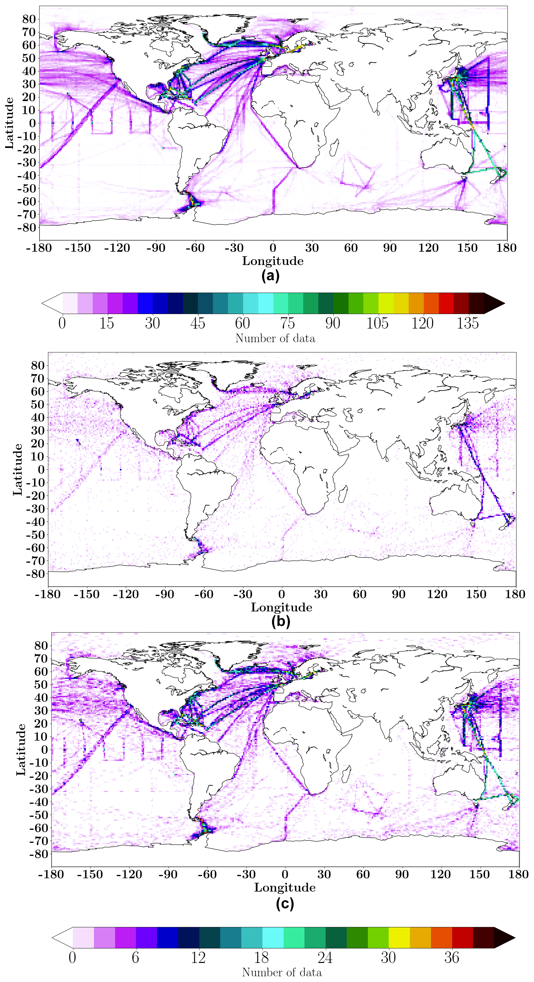
Figure 1 Spatial distribution of SOCAT data (number of measurements per grid point): (a) for the 2001–2016 period; (b) for all months of January for the 2001–2016 period; (c) for all months of December–January–February for the 2001–2016 period. Please note that the color bar under panel (c) refers to both (b) and (c).

c The following formula is used to convert fCO₂ to pCO₂ (Körtzinger, 1999):

$$\begin{array}{}\text{(1)}& {\displaystyle }f{\mathrm{CO}}_{\mathrm{2}}=p{\mathrm{CO}}_{\mathrm{2}}\exp \left(p{\displaystyle \frac{B+\mathrm{2}\mathit{\delta }}{RT}}\right),\end{array}$$

where fCO₂ and pCO₂ are in micro-atmospheres (µatm), p is the total pressure (Pa), R=8.314 J K⁻¹ is the gas constant and T is the absolute temperature (K). Parameter B (m³ mol⁻¹) is estimated as $B=(-\mathrm{1636.75}+\mathrm{12.040}T-\mathrm{3.27957}\times {\mathrm{10}}^{-\mathrm{2}}{T}^{\mathrm{2}}+\mathrm{3.16528}$ $\times {\mathrm{10}}^{-\mathrm{5}}{T}^{\mathrm{3}})\times {\mathrm{10}}^{-\mathrm{6}}$. The parameter δ is the cross-virial coefficient (m³ mol⁻¹): $\mathit{\delta }=\left(\mathrm{57.7}-\mathrm{0.118}T\right)\times {\mathrm{10}}^{-\mathrm{6}}$. The total pressure is from the Jena database (6 h, $\mathrm{5}{}^{\circ }\times \mathrm{5}{}^{\circ }$; http://www.bgc-jena.mpg.de/CarboScope/?ID=s, last access: 13 September 2017) based on the National Center for Environmental Prediction (NCEP) reanalysis (Kalnay et al., 1996) .

Monthly global reprocessed products of physical variables from ARMOR3D L4 distributed through the Copernicus Marine Environment Monitoring Service (CMEMS; $\mathrm{0.25}{}^{\circ }\times \mathrm{0.25}{}^{\circ }$; http://marine.copernicus.eu/services-portfolio/access-to-products/?option=com_csw&view=details&product_id=MULTIOBS_GLO_PHY_REP_015_002, last access: 27 October 2017) were used for SSS, SST and SSH (Guinehut et al., 2012). The GlobColour project provided monthly chlorophyll (GlobColour “CHL” data) distributions at a $\mathrm{1}{}^{\circ }\times \mathrm{1}{}^{\circ }$ resolution (http://www.globcolour.info/products_description.html, last access: 31 October 2017). For MLD, daily data from the “Estimating the Circulation and Climate of the Ocean” (ECCO2) project Phase II (Cube 92), at a $\mathrm{0.25}{}^{\circ }\times \mathrm{0.25}{}^{\circ }$ resolution (Menemenlis et al., 2008) were used. For atmospheric xCO₂, the 6h data from Jena CO₂ inversion s76_v4.1 on a $\mathrm{5}{}^{\circ }\times \mathrm{5}{}^{\circ }$ grid were selected (http://www.bgc-jena.mpg.de/CarboScope/?ID=s, last access: 13 September 2017). Finally, an ice mask based on daily “Operational Sea Surface Temperature and Sea Ice Analysis” (OSTIA) data with a gridded $\mathrm{0.05}{}^{\circ }\times \mathrm{0.05}{}^{\circ }$ resolution (Donlon et al., 2011) was applied.

MLD and CHL data were log-transformed before their use in the FFNN algorithm because of their skewed distribution. In regions with no CHL data (high latitudes in winter) log(CHL) =0 was applied. It does not introduce discontinuities, as log(CHL) is close to zero in the adjacent region.

All data were averaged or interpolated on a $\mathrm{1}{}^{\circ }\times \mathrm{1}{}^{\circ }$ grid and, depending on the resolution of the dataset, averaged over the month. It is worth noting that all datasets have to be normalized (i.e., centered to zero-mean and reduced to unit standard deviation) before their use in the FFNN algorithm, for example,

$${\displaystyle }{\text{SSS}}_n={\displaystyle \frac{\text{SSS}-\stackrel{\mathrm{‾}}{\text{SSS}}}{\text{SD}\left(\text{SSS}\right)}}.$$

Normalization ensures that all predictors fall within a comparable range and avoids giving more weight to predictors with large variability ranges (Kallache et al., 2011).

As surface ocean pCO₂ also varies spatially, geographical positions, latitude (lat) and longitude (long), after conversion to radians were included as predictors. In order to normalize (lat, long) the following transformation is proposed:

$$\begin{array}{ll}{\displaystyle }& {\displaystyle }{\text{lat}}_n=\sin \left(\text{lat}\cdot \mathit{\pi }/\mathrm{180}{}^{\circ }\right)\\ {\displaystyle }& {\displaystyle }{\text{long}}_{n,\mathrm{1}}=\sin \left(\text{long}\cdot \mathit{\pi }/\mathrm{180}{}^{\circ }\right)\\ {\displaystyle }& {\displaystyle }{\text{long}}_{n,\mathrm{2}}=\cos \left(\text{long}\cdot \mathit{\pi }/\mathrm{180}{}^{\circ }\right)\end{array}$$

Two functions sin and cos for longitudes are used to preserve its periodical 0 to 360^∘ behavior and thus to consider the difference of positions before and after the 0^∘ longitude. For step 2, data required for training were colocated at the SOCAT data positions that are used as a target for the FFNN model. Details are provided in the next section.

2.2 Methods

2.2.1 Network configuration and evaluation protocol

In this work, we use Keras, a high-level neural network Python library (“Keras: the Python Deep Learning library”, Chollet, 2015; https://keras.io) to build and train the FFNN models. The identification of an optimal configuration is the first step in the FFNN model building. This includes the choice of the number and size of hidden layers (i.e., intermediate layers between input and output layers), the connection type, the activation functions, the loss function and optimization algorithm, as well as the learning rate and other low-level parameters. Based on a series of tests and their statistical results (RMSE, correlation and bias) a hyperbolic tangent was chosen as an activation function for neurons in hidden layers, and a linear function was chosen for the output layer. As an optimization algorithm, the mini-batch gradient descent or “RMSprop” was used (adaptive learning rates for each weight, Chollet, 2015; Hinton et al., 2012). The number of layers and neurons utilized depends on the problem. For totally connected layers (i.e., a neuron in a hidden layer is connected to all neurons in the precedent layer and connects all neurons in the next one), which is the case here, it is enough to have only one single hidden layer, although two or more can help the approximation of complex functions (or complex relationships between the input and the output of the problem).

The number of FFNN layers and the number of neurons depends on the complexity of the problem: the more layers and neurons, the better the accuracy of the output. However, the size also depends on the number of patterns (data) used for training. The empirical rule recommends having a factor of 10 between the number of patterns (data) and the number of connections, or weights to adjust (in line with Amari et al., 1997, we use a factor of 10 that necessitates a cross-validation to avoid overfitting). This limits the size, the number of parameters and incidentally the number of neurons of the FFNN. This empirical rule was followed in this study.

1. Step 1: reconstruction of monthly climatologies. FFNN reconstructs a normalized monthly surface ocean pCO₂ climatology as a nonlinear function of normalized SSS, SST, SSH, Chl a, MLD climatologies and geographical position (lat and long):

   $$\begin{array}{ll}{\displaystyle }& {\displaystyle }{p\mathrm{CO}}_{\mathrm{2},n}\\ \text{(2)}& {\displaystyle }& {\displaystyle }=\left({\text{SSS}}_n,{\text{SST}}_n,{\text{SSH}}_n,{\mathrm{Chl}}_n,{\text{MLD}}_n,{\text{long}}_n,{\text{lat}}_n\right).\end{array}$$

   Surface ocean pCO₂ from Takahashi et al. (2009) provided the target. The dataset was divided into 50 % for FFNN training and 25 % for its evaluation. This 25 % did not participate in the training. This set is used to monitor the performance of the training process and to drive its convergence. The remaining 25 % (each fourth point) of the dataset was used after training for the FFNN model validation. More details about the FFNN training process can be found in Rumelhart et al. (1986) and Bishop (1995). Validation and evaluation datasets were chosen quasi-regularly in space and time to take all regions and seasonal variability into account. In order to improve the accuracy of the reconstruction, the model was applied separately for each month. We have developed a FFNN model with five layers (three hidden layers). Twelve models with a common architecture were trained. Tests with one model for 12 months showed a slight decrease in accuracy (not presented here). About 17 500 data were available for each month to train the model, resulting in monthly FFNN models with about 1856 parameters.

2. Step 2: reconstruction of anomalies. During the second step, normalized pCO₂ anomalies were reconstructed as a nonlinear function of normalized SSS, SST, SSH, Chl a, MLD, xCO₂ and their anomalies, as well as geographic position:

   $$\begin{array}{ll}{\displaystyle }& {\displaystyle }{p\mathrm{CO}}_{\mathrm{2},\mathrm{anom},n}\\ {\displaystyle }& {\displaystyle }=\left({\text{SSS}}_n,{\text{SST}}_n,{\text{SSH}}_n,{\mathrm{Chl}}_n,{\text{MLD}}_n,{x\mathrm{CO}}_{\mathrm{2},n},\right.\\ {\displaystyle }& {\displaystyle }{\text{SSS}}_{\mathrm{anom},n},{\text{SST}}_{\mathrm{anom},n},{\text{SSH}}_{\mathrm{anom},n},{\mathrm{Chl}}_{\mathrm{anom},n},\\ \text{(3)}& {\displaystyle }& {\displaystyle }\left.{\text{MLD}}_{\mathrm{anom},n},{x\mathrm{CO}}_{\mathrm{2},\mathrm{anom},n},{\text{long}}_{n,\mathrm{1}},{\text{long}}_{n,\mathrm{2}},{\text{lat}}_n\right)\end{array}$$

   Surface ocean pCO₂ anomalies were computed as the differences between colocated pCO₂ values based on SOCAT observations and monthly pCO₂ climatologies reconstructed during the first step that provided the targets:

   $$\begin{array}{}\text{(4)}& {\displaystyle }{p\mathrm{CO}}_{\mathrm{2},\mathrm{anom}}={p\mathrm{CO}}_{\mathrm{2},\mathrm{SOCAT}}-{p\mathrm{CO}}_{\mathrm{2},\mathrm{clim},\mathrm{FFNN}}.\end{array}$$

   The set of target data was again divided into 50 % for the training algorithm, 25 % for evaluation and 25 % for model validation. As in step (1) the model was trained separately for each climatological month. Thus, there were 12 models sharing a common architecture but trained on different data. In this step, in order to increase the amount of data during training and introduce information on the seasonal cycle, the model was trained using pCO₂ data from the month in question as a target as well as data from the previous and following month during the entire period from 2001 to 2016. Figure 1b and c show an example of the data distribution for the months of January over the period from 2001 to 2016 (Fig. 1b) and for the 3-month time window including December–January–February from 2001 to 2016 used in the training algorithm of the January FFNN model (Fig. 1c). In this particular example, the choice of 3 months provided a better cover of the region and doubled the number of data at high latitudes.

K-fold cross-validation was used for the evaluation and the validation of the FFNN architecture. Cross-validation relied on K=4 different subsamples of the dataset to draw 25 % of independent data for validation (Fig. S1 in the Supplement). Each sampling fold was tested on five runs of the FFNN for each month. Each of these five runs was characterized by different initial values that were randomly chosen. From these five results, the best was chosen based on root-mean-square error (RMSE), the r² and the bias.

The final model architecture at step 2 had three layers (one hidden layer). About 10 000 samples were available for training for each month; thus, a model with 541 parameters was developed. Note that a higher number of parameters did not show a significant improvement in the accuracy.

2.2.2 Reconstruction of surface ocean pCO₂

The previous section presented the development of the “optimal” architecture of a FFNN model for the reconstruction of global surface ocean pCO₂ and the estimation of its accuracy. This FFNN model was used to provide the final product for scientific analysis and comparison with other mapping approaches. In order to provide the final output, the selected FFNN architecture was trained on all available data: 100 % of data for training, 100 % for evaluation and 100 % for validation. The network was executed five times (different initial values) and the best model was selected based on validation results considering the root-mean-square error (RMSE), the r² and the bias computed between the network output and the SOCAT-derived surface ocean pCO₂ data. The final model output is referred to as the LSCE-FFNN product.

2.3 Computation of sea–air CO₂ fluxes

The sea–air CO₂ flux, f, was calculated following Rödenbeck et al. (2015) as

$$\begin{array}{}\text{(5)}& {\displaystyle }f=k\mathit{\rho }L\left(p{\mathrm{CO}}_{\mathrm{2}}-p{\mathrm{CO}}_{\mathrm{2}}^{\mathrm{atm}}\right),\end{array}$$

where k is the piston velocity estimated according to Wanninkhof (1992):

$$\begin{array}{}\text{(6)}& {\displaystyle }k=\mathrm{\Gamma }{u}^{\mathrm{2}}{\left({\mathit{\text{Sc}}}^{{\mathrm{CO}}_{\mathrm{2}}}/{\mathit{\text{Sc}}}^{\mathrm{Ref}}\right)}^{-\mathrm{0.5}}.\end{array}$$

The global scaling factor Γ was chosen as in Rödenbeck et al. (2014) with the global mean CO₂ piston velocity equaling 16.5 cm h⁻¹. Sc corresponds to the Schmidt number estimated according to Wanninkhof (1992). The wind speed was computed from 6-hourly NCEP wind speed data (Kalnay et al., 1996). ρ is seawater density in Eq. (5) and L is the temperature-dependent solubility (Weiss, 1974). pCO₂ corresponds to the surface ocean pCO₂ output of the mapping method. $p{\mathrm{CO}}_{\mathrm{2}}^{\mathrm{atm}}$ was derived from the atmospheric CO₂ mixing ratio fields provided by the Jena inversion s76_v4.1 (http://www.bgc-jena.mpg.de/CarboScope/).

3 Results

3.1 Validation

The subset of data used for network validation, which was 25 % of the total, represented independent observations, as they did not participate in training during model development (see Section 2.2.1). The skill of the FFNN to reconstruct monthly climatologies of surface ocean pCO₂ was assessed by comparing colocated reconstructed pCO₂ and corresponding values from Takahashi et al. (2009). The global climatology was reconstructed with satisfying accuracy during step 1 with a RMSE of 0.17 µatm and an r² of 0.93. The model output of step 2 was assessed using K-fold cross-validation as previously presented: K=4 different subsets of independent data were drawn from the dataset and the network was run five times on each subset. From these 20 results the best one was chosen based on the RMSE, the r² and mean absolute error (MAE) (the bias is presented in Table S1 in the Supplement). A combination of the four best model output was used for the statistical analysis summarized in Table 1. Metrics were computed over the full period (2001–2016) and with reference to SOCAT observations (independent data only). At the global scale, the analysis yielded a RMSE of ∼17.97 µatm, whereas the MAE was 11.52 µatm and the r² was 0.76. These results were comparable to those obtained by Landschützer et al. (2013) for the assessment of a surface ocean pCO₂ reconstruction based on an alternative neural network-based approach. The RMSE between the SOCAT data and the pCO₂ climatology from Takahashi et al. (2009) equalled 41.87 µatm, which was larger than errors computed for the regional comparison between FFNN and SOCAT (Table 1). We also estimated the RMSE for the case where 100 % of the data were used for training, which equalled 14.8 µatm and confirmed the absence of overfitting.

Table 1 Statistical validation of LSCE-FFNN. Comparison between reconstructed surface ocean pCO₂ and pCO₂ values from the SOCAT v5 database not used in the training algorithm for the period from 2001 to 2016 over the global ocean (except for regions with ice cover) and for large oceanographic regions. The number of measurements per region is given in parentheses in the first column.

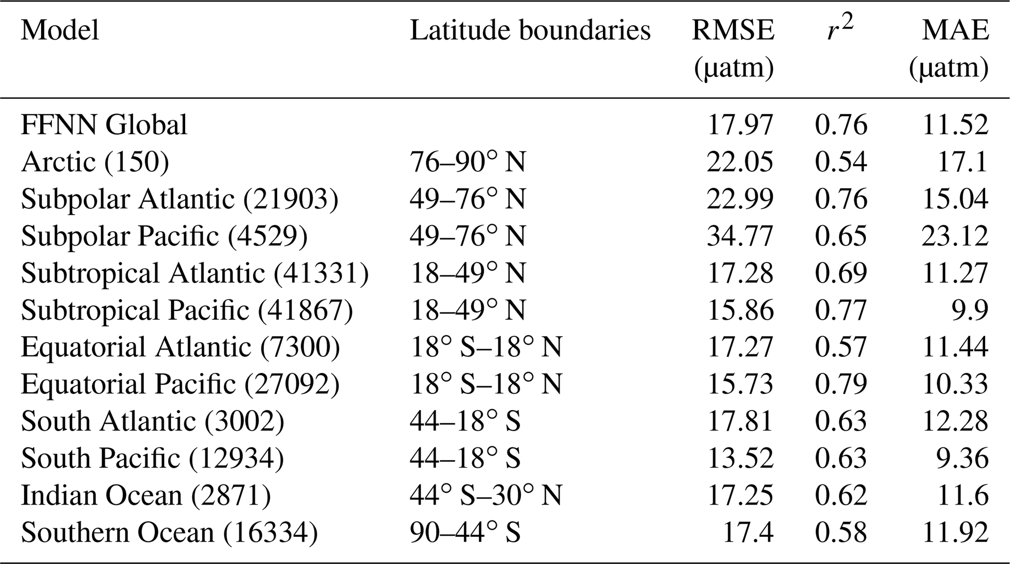
Figure 2a shows the time mean difference between the estimated pCO₂ and pCO₂ from SOCAT v5 data used for validation: ${\text{mean}}_t\left({p\mathrm{CO}}_{\mathrm{2},i,j,\mathrm{FFNN}}-{p\mathrm{CO}}_{\mathrm{2},i,j,\mathrm{SOCAT}}\right)$. Large differences occurred at high latitudes, in equatorial regions, and along the Gulf Stream and Kuroshio currents – the regions with strong horizontal gradients of pCO₂. Moreover, the standard deviation of the residuals (Fig. 2b) in these regions was larger, indicating that the model fails to accurately reproduce the temporal variability. The reduced skill of the model in these regions reflects the poor data coverage along with a strong seasonal variability (e.g., the Southern Ocean) and/or high kinetic energy (e.g., the Southern Ocean and the Kuroshio and Gulf Stream currents) (Fig. 1a). At the scale of oceanic regions, (Table 1) the largest RMSE and MAE values were computed for the Pacific subpolar ocean (RMSE =34.77 µatm and MAE =23.12 µatm), whereas the lowest correlation coefficient was obtained for the equatorial Atlantic Ocean (r²=0.57). These low scores directly reflect low data density and are to be contrasted with those obtained over regions with better data coverage (e.g., the subtropical North Pacific with RMSE =15.86 µatm, MAE =9.9 µatm and r²=0.77, or the subpolar Atlantic with RMSE =22.99 µatm, MAE =15.04 µatm and r²=0.76). Despite large time mean differences computed over the eastern equatorial Pacific, scores are satisfying at the regional scale indicating error compensation by improved scores over the western basin (RMSE =15.73 µatm, MAE =10.33 µatm and r²=0.79). Scores are low in the Southern Hemisphere (Table 1) and time mean differences are large (Fig. 2a) reflecting sparse data coverage (Fig. 1a).

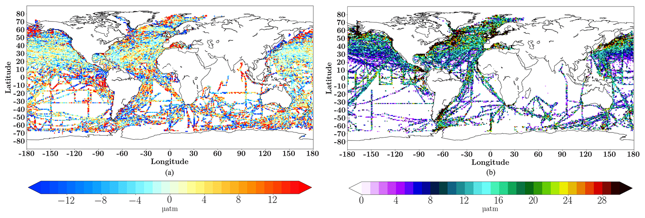
Figure 2 Time mean differences (µatm) between monthly LSCE-FFNN pCO₂ and SOCAT pCO₂ data used for evaluation of the model over the period from 2001 to 2016 (a) and its standard deviation (b).

3.2 Qualification

This section presents the assessment of the final time series of reconstructed surface ocean pCO₂. The time series was computed using the best monthly models as described in Sect. 2.2, as well as 100 % of the data for learning, evaluation and validation.

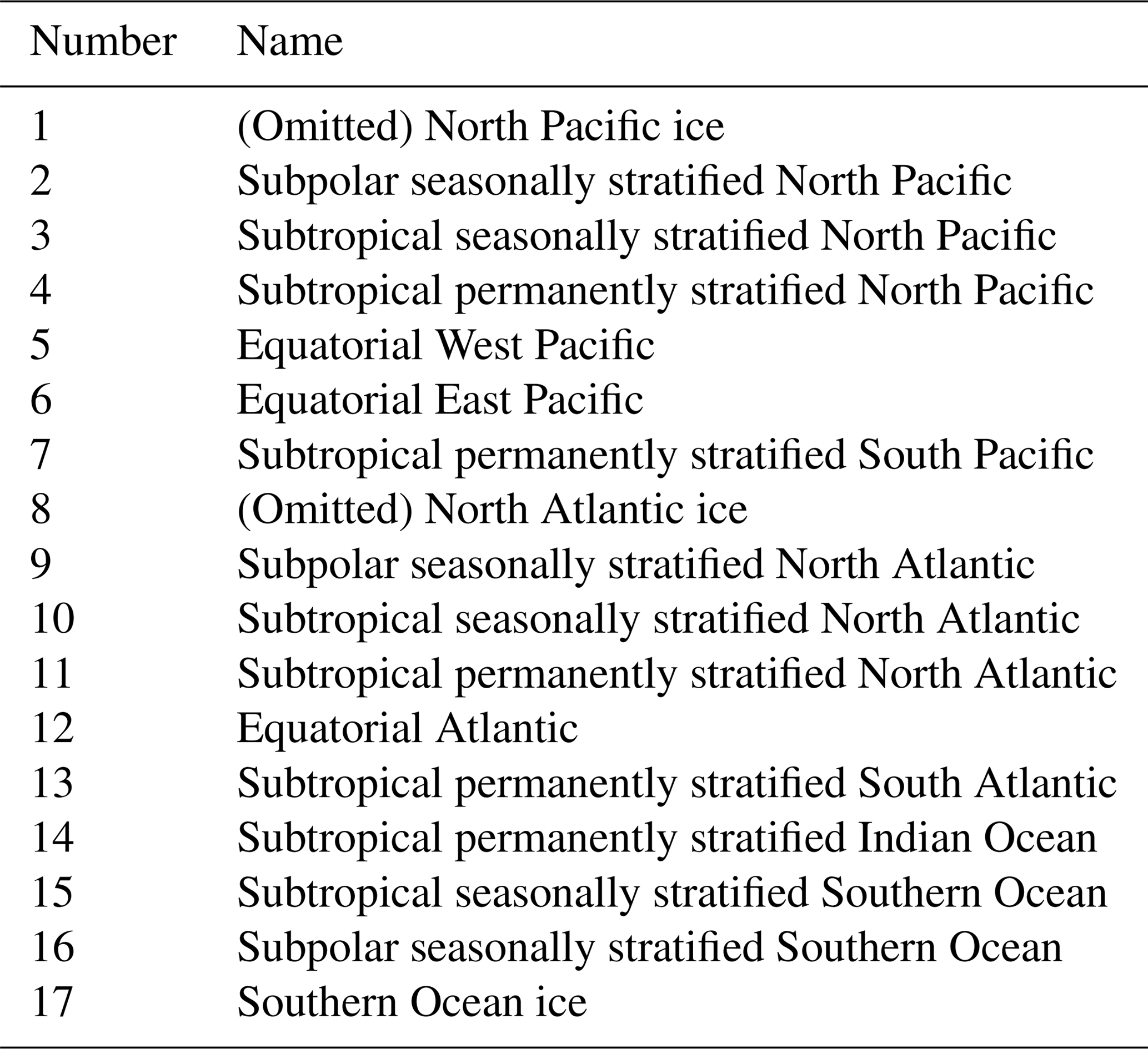
Results of the LSCE-FFNN mapping model were compared to three published mapping methods which participated in the “Surface Ocean pCO2 Mapping Intercomparison” (SOCOM) exercise presented in Rödenbeck et al. (2015) (http://www.bgc-jena.mpg.de/SOCOM/). These methods are as follows: (1) Jena-MLS oc_v1.5 (Rödenbeck et al., 2014), which is a statistical interpolation scheme (data-driven mixed-layer scheme; principal drivers used in parameterization: ocean-internal carbon sources/sinks, SST, wind speed, mixed-layer depth climatology and alkalinity climatology); (2) JMA-MLR (updated version up to 2016) (Iida et al., 2015), which is based on multi-linear regressions with SST, SSS and Chl a as independent variables; and (3) ETH-SOMFFN v2016 (Landschützer et al., 2014), which is a two-step neural network model with SST, SSS, MLD, Chl a and xCO₂ as drivers. The time series of pCO₂ and sea–air CO₂ flux (f) were assessed over 17 biomes defined by Fay and McKinley (2014) (Fig. 3, Table 2). These biomes were derived based on coherence in SST, Chl a, the ice fraction, and the maximum MLD and represent regions of coherent biogeochemical dynamics.

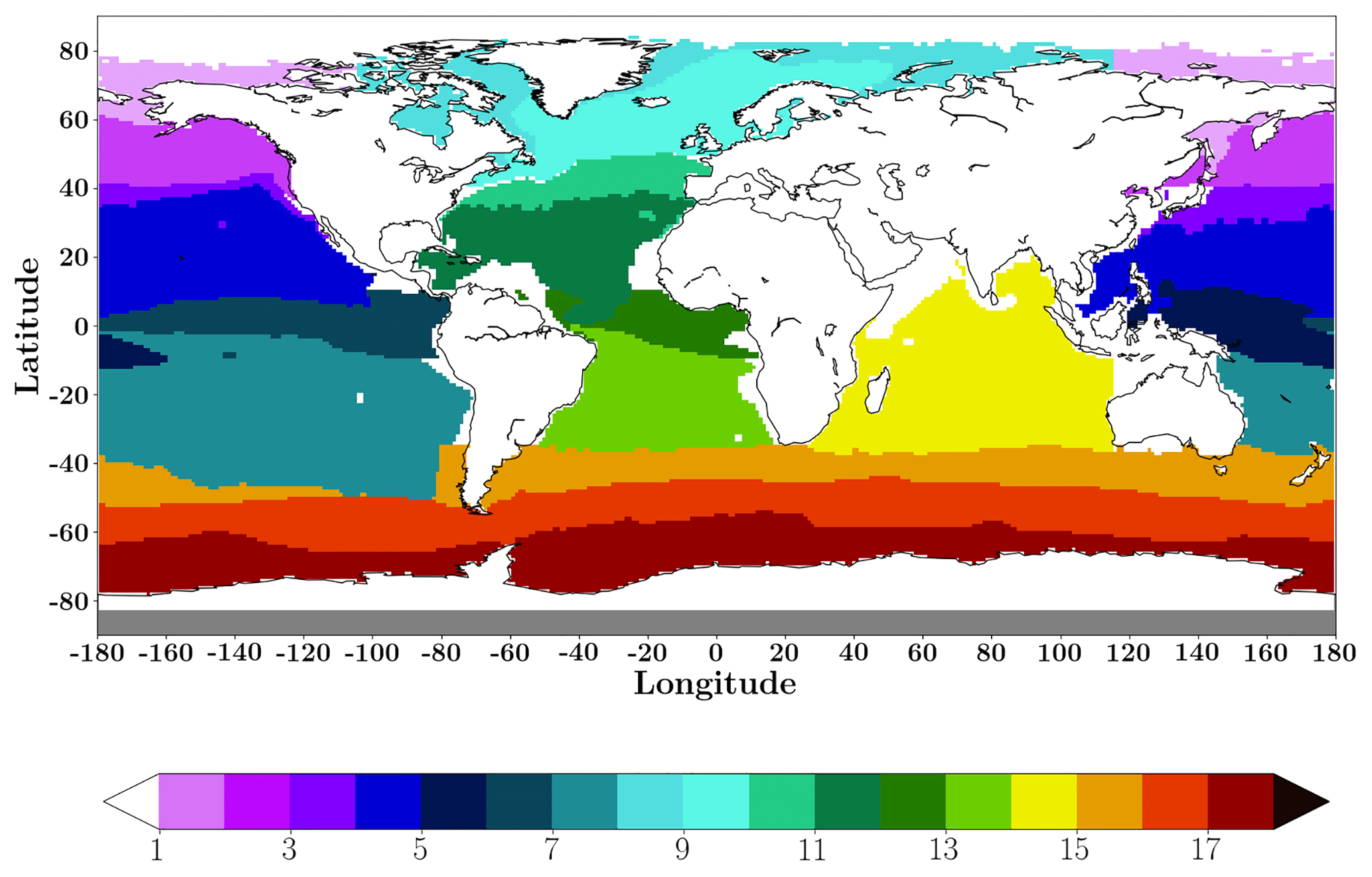
Figure 3 Map of biomes (following Rodenbeck et al., 2015; Fay and McKinley, 2014) used for comparison. See Table 2 for biome names.

We followed the protocol and diagnostics proposed in Rödenbeck et al. (2015) for the comparison of each of the respective mapping methods with one another, with respect to observations. The following diagnostics were computed: (1) the relative interannual variability (IAV) mismatch R^iav (in percent), and (2) the amplitude of interannual variations. The relative interannual variability (IAV) mismatch R^iav (in percent) is the ratio of the mismatch amplitude M^iav of the difference between the model output and the observations (its temporal standard deviation) and the mismatch amplitude $M_{\mathrm{benchmark}}^{\mathrm{iav}}$ of the “benchmark”. The latter was derived from the mean seasonal cycle of the corresponding model output where the trend of increasing yearly atmospheric pCO₂ was added (see details in Rödenbeck et al., 2015). It corresponds to a climatology corrected for increasing atmospheric CO₂, but without interannual variability.

$$\begin{array}{}\text{(7)}& {\displaystyle }{R}^{\mathrm{iav}}={\displaystyle \frac{M^{\mathrm{iav}}}{M_{\mathrm{benchmark}}^{\mathrm{iav}}}}\cdot \mathrm{100}\mathit{\%},\end{array}$$

where

$$\begin{array}{ll}{\displaystyle }& {\displaystyle }{M}^{\mathrm{iav}}=\text{SD}\left(\text{mean}\left(p{\mathrm{CO}}_{\mathrm{2},\mathrm{Model}}-p{\mathrm{CO}}_{\mathrm{2},\mathrm{SOCAT}}\right)\right),\\ {\displaystyle }& {\displaystyle }{M}_{\mathrm{benchmark}}^{\mathrm{iav}}=\text{SD}\left(\text{mean}\left(D_{\mathrm{season}}\right)\right).\end{array}$$

Here “mean” is a mean over the region and year, and

$${\displaystyle }{D}_{\mathrm{season}}=\left(p{\mathrm{CO}}_{\mathrm{2},\mathrm{SS}}+\text{trend}\left({\mathrm{CO}}_{\mathrm{2},\mathrm{atm}}\right)\right)-p{\mathrm{CO}}_{\mathrm{2},\mathrm{SOCAT}},$$

pCO_2, SS is the seasonal cycle of pCO₂ from the corresponding mapping method. CO_2, atm estimates from xCO₂ Jena CO₂ inversion s76_v4.1 were used.

Table 2 Biomes from Fay and McKinley (2014) used for time series comparison (Fig. 3).

R^iav provides information on the capability of each method to reproduce the IAV compared to observations: a smaller R^iav represents a better fit compared with the reference. The amplitude of the interannual variations (A^iav) of sea–air flux of CO₂ (its 2-month running mean) is estimated as the temporal standard deviation over the period.

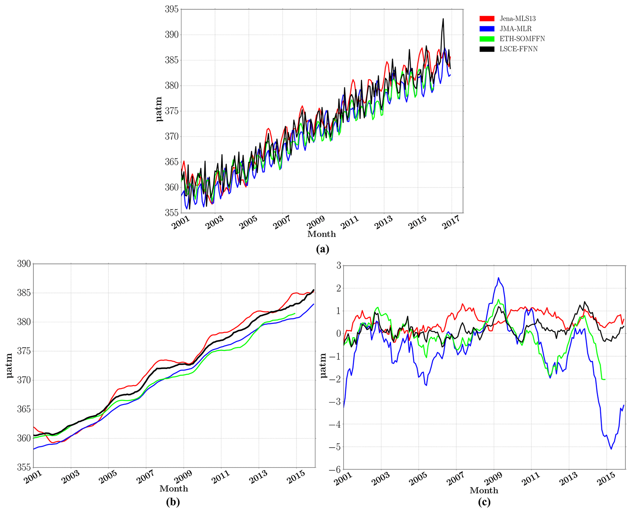
Figure 4 Global oceanic pCO₂: Jena (red), JMA (blue), ETH-SOMFFN (green) and LSCE-FFNN (black). (a) Global average monthly time series, (b) the global 12-month running mean average and (c) yearly pCO₂ mismatch (difference between mapping methods and SOCAT data).

3.2.1 Interannual variability

The time series of globally averaged surface ocean pCO₂ over the period from 2001 to 2016 are presented in Fig. 4 for LSCE-FFNN and the three other models. Surface ocean pCO₂ (µatm) varied between the four mapping methods in the range of ±7 µatm (Fig. 4a). Modeled pCO₂ values were at the lower end for ETH-SOMFFN and JMA-MLR, whereas LSCE-FFNN and Jena-MLS13 computed higher values. The same behavior was found for the 12-month running mean time series (Fig. 4b). Figure 4c shows the 12-month running mean of the difference between computed pCO₂ and SOCAT data (model – SOCAT) over the globe. JMA-MLR mostly underestimated observed pCO₂ with a strong interannual variability of the misfit, especially at the end of the period, with up to −5 µatm. The difference between ETH-SOMFFN output and SOCAT data fluctuated in the range of ±1 µatm, with an increase in amplitude up to −2 µatm from 2010 onward. Jena-MLS13 overestimated observations with the difference in the range of 0–1 µatm. The difference between LSCE-FFNN and SOCAT varied around zero (between −0.7 and 1 µatm).

The model was then assessed at biome scale. Results for all biomes are presented in the Supplement (Figs. S2, S3, S4). Two biomes with contrasting dynamics are discussed hereafter in greater detail: (1) the equatorial East Pacific (biome 6) characterized by a strong IAV of surface ocean pCO₂ and sea–air CO₂ fluxes in response to ENSO, the El Niño–Southern Oscillation (Feely et al., 1999; Rödenbeck et al., 2015), and (2) the North Atlantic permanently stratified biome (biome 11) with a well-marked seasonal cycle, but little IAV (Schuster et al., 2013). Results for these biomes are presented in Fig. 5.

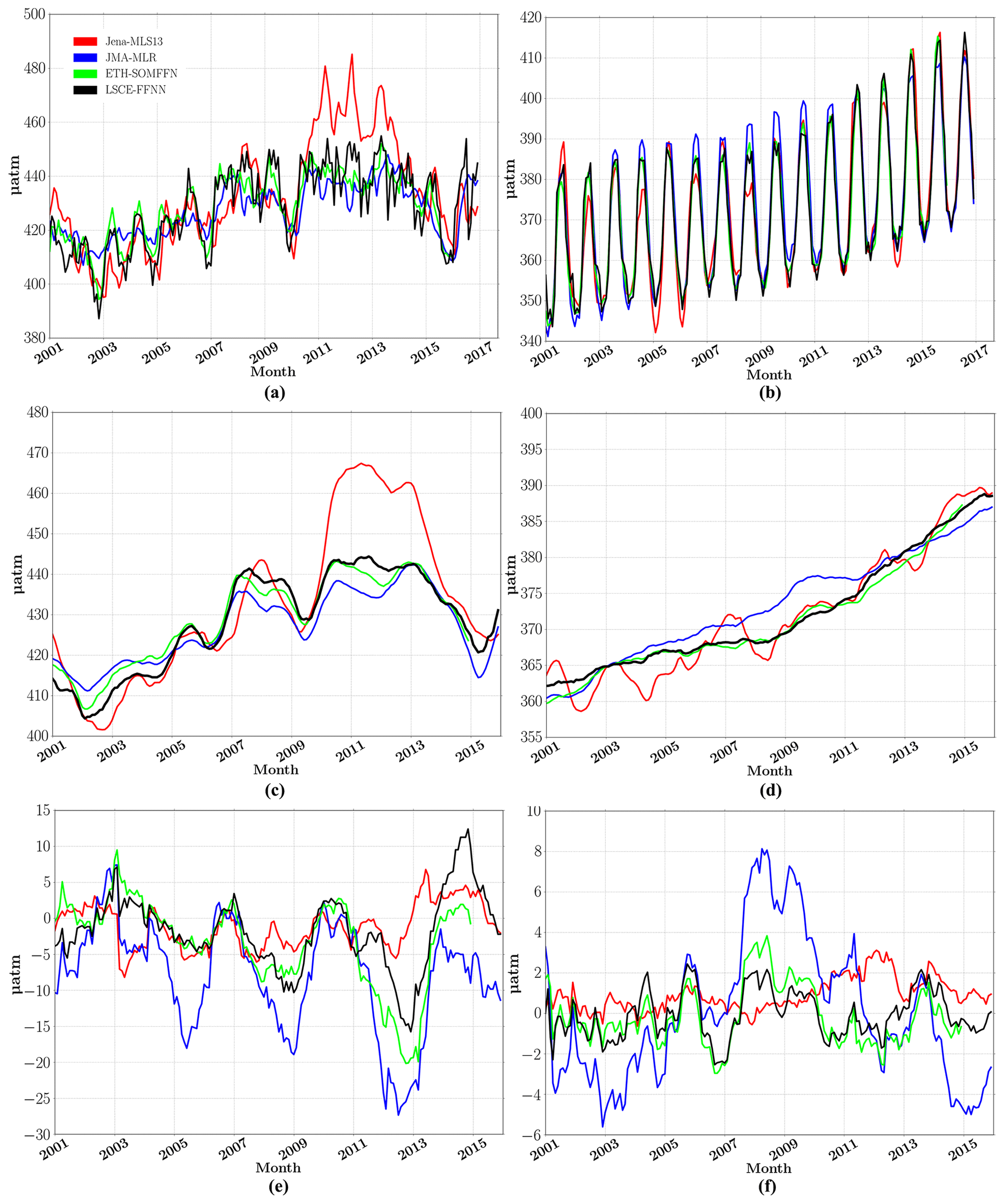
Figure 5 Surface ocean pCO₂ in the equatorial East Pacific (biome 6) (a, c, e) and the subtropical permanently stratified North Atlantic (biome 11) (b, d, f): FFNN (black), JMA (blue), Jena (red) and ETH-SOMFFN (green). (a, b) The monthly time series averaged over the biome. (c, d) The 12-month running mean averaged over the biome. (e, f) The yearly pCO₂ mismatch (difference between the mapping methods and the SOCAT data).

Biome 6 is relatively well-covered by observations and represents a key region for testing the skill of the model to reproduce the observed strong IAV linked to ENSO. El Niño events are characterized by positive SST anomalies, reduced upwelling and decreased surface ocean pCO₂ values. These episodes could be identified in all model time series (Fig. 5a) with reduced pCO₂ levels in 2004/05 and 2006/07 (weak El Niño), 2002/03 and 2009/10 (moderate El Niño), and 2015/16 (strong El Niño). JMA-MLR (blue curve in Fig. 5a) tended to underestimate pCO₂ during weak El Niño events; it was also underestimated during the La Niña 2011–2012 event by Jena-MLS13. LSCE-FFNN and ETH-SOMFFN, both based on a neural network approach, yielded similar results despite differences in network architecture and predictor datasets.

Data coverage is particularly high over Biome 11 (Fig. 5b, d, f). The seasonal cycle in this biome is dominantly driven by temperature. Modeled seasonal variability showed good agreement across the ensemble of methods (Fig. 5b) with an increase in spring–summer and a decrease in autumn–winter. However, the amplitude can be different by up to 10 µatm between different models. The seasonal amplitude of pCO₂ computed by JMA-MLR increased from smaller values at the beginning of the time series to higher values in the middle of the 2005–2012 period. The variability of seasonal amplitude was the highest for Jena-MLS13 in line with the 12-month running mean time series (Fig. 5d). Again, similar seasonal amplitude and year-to-year variability of surface ocean pCO₂ were obtained with LSCE-FFNN and ETH-SOMFFN (Fig. 5b, d). The yearly pCO₂ mismatch (Fig. 5f) shows that observed surface ocean pCO₂ was underestimated by JMA-MLR at the beginning and at the end of the period by up to −6 µatm, and overestimated during the 2007–2011 period by up to 8 µatm. Jena-MLS13 shows mostly positive differences in the range of 0–2 µatm over the full period. LSCE-FFNN and ETH-SOMFFN vary around zero and between −2 and 2 µatm, respectively, and are close to each other.

3.2.2 Sea–air CO₂ flux variability

Sea–air exchange of CO₂ was estimated using the same gas-exchange formulation (Eq. 5) and wind speed data (6-hourly NCEP wind speed) for each mapping data (Rödenbeck et al., 2005). It is worth noting that the sea–air flux is sensitive to the choice of the wind speed dataset (Roobaert et al., 2018).

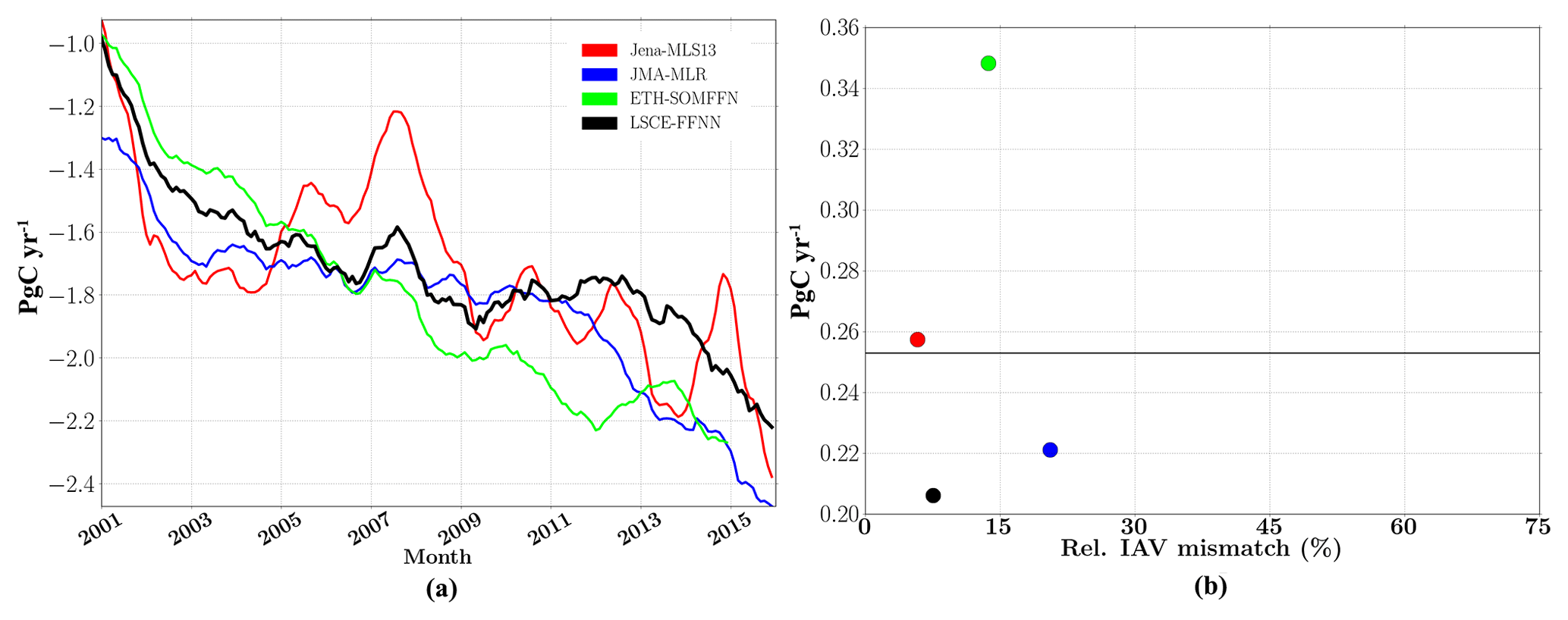
Figure 6 (a) Interannual global ocean sea–air CO₂ flux (12-month running mean); (b) the amplitude of interannual CO₂ flux plotted against the relative IAV mismatch amplitude. The weighted mean is given as a horizontal line.

Figure 6a presents the global 12-month running mean of the sea–air CO₂ flux for four mapping methods. All models showed an increase in CO₂ uptake in response to increasing atmospheric CO₂ levels, albeit with a strong between-model variability in multi-annual trends. There is less agreement between the methods compared to reconstructions of surface ocean pCO₂ variability (Fig. 4b). This results from the contribution of uncertainties in sea–air CO₂ flux estimations over regions with poor data coverage (mostly in the South Hemisphere: the South Pacific, the South Atlantic, the Indian Ocean and the South Ocean; see Fig. S5). Nevertheless, the relative IAV mismatch was less than 30 % for all methods (Fig. 6b), suggesting a reasonable fit to observational data. However, the relative IAV mismatch is a global score, and it is biased towards regions with good data coverage (Rödenbeck et al., 2015). The time series reconstructed in this study is too short to capture decadal variations and, in particular, the strengthening of the sink from 2000 onward (Landschützer et al., 2016). LSCE-FFNN computed a slowdown of ocean CO₂ uptake between 2010 and 2013 with a flux of $\sim -\mathrm{1.8}$ GtC yr⁻¹ compared with $\sim -\mathrm{2.2}$ GtC yr⁻¹ for ETH-SOMFFN. A leveling-off was also found for JMA-MLR, albeit shifted in time. In general, the amplitudes of reconstructed CO₂ fluxes across all four methods agreed within 0.2 to 0.36 PgC yr⁻¹. The weighted mean of IAV (horizontal line in Fig. 6b) computed from the four methods included here was 0.25 PgC yr⁻¹. This value is close to that reported by Rödenbeck et al. (2015) for the complete ensemble of SOCOM models (0.31 PgC yr⁻¹) estimated for the period from 1992 to 2009. The largest amplitude was obtained for ETH-SOMFFN (∼0.35 PgC yr⁻¹). Conversely, LSCE-FFNN has the smallest amplitude with 0.21 PgC yr⁻¹. Jena-MLS13 and JMA-MLR lie very close to the weighted mean value with 0.26 and 0.22 PgC yr⁻¹, respectively. The weighted mean and the dispersion of individual models around it, reflect the period of analysis (2001–2015; ETH-SOMFFN output provided up to 2015) and the total number of models contributing to it (see Rödenbeck et al., 2015 for comparison). As such, it does not provide information on the skill of any particular model.

The interannual variability of reconstructed sea–air CO₂ fluxes (12-month running mean) showed good agreement for biome 6 (East Pacific equatorial, Fig. 7a). A small discrepancy was found at the beginning of the period. A strong increase was computed by Jena-MLS13 for 2010–2014 that was also identified in the pCO₂ variability (Fig. 5a). Despite this, Jena-MLS13 had a low relative R^IAV (26 %), which confirmed a tendency mentioned in Rödenbeck et al. (2015): that mapping products with a small relative IAV mismatch show larger amplitude. LSCE-FFNN and ETH-SOMFFN yielded comparable results (Fig. 7a, c) with relative IAV mismatches of 46 % and 53 %, respectively, and with amplitudes of ∼0.03 PgC yr⁻¹. Interannual variability reproduced by JMA-MLR falls within the range of the other models (Fig. 7c), but with a R^IAV of ∼68 %.

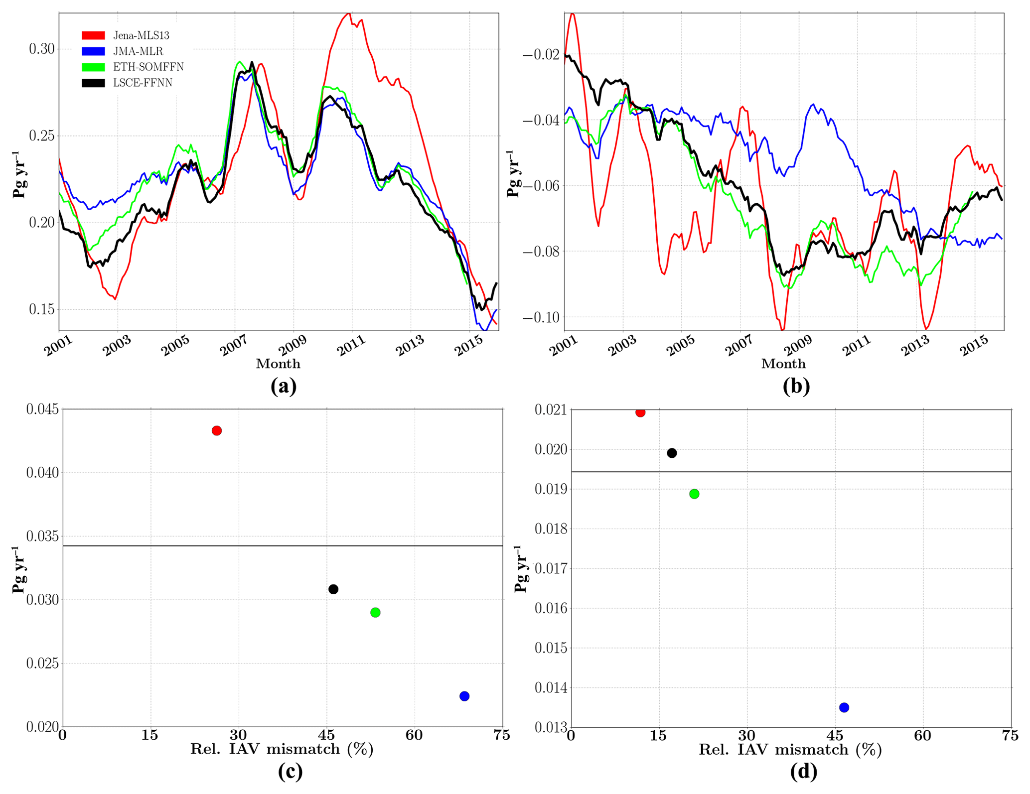
Figure 7 Global ocean interannual sea–air CO₂ flux (12-month running mean) in (a)  the equatorial East Pacific (biome 6) and (b)  the subtropical permanently stratified North Atlantic (biome 11). The amplitude of interannual CO₂ flux plotted against the relative IAV mismatch amplitude in (c) the equatorial East Pacific (biome 6) and (d) the subtropical permanently stratified North Atlantic (biome 11). The weighted mean is given as a horizontal line.

Reconstructed sea–air CO₂ fluxes over the North Atlantic subtropical permanently stratified region (biome 11) show large between model differences in amplitudes and variability. The two models based on a neural network again show good agreement with an R^IAV of 17 % for LSCE-FFNN and 20 % for ETH-SOMFFN. Jena-MLS13 produced a strong seasonal variability (Fig. 7b) up to 0.06 PgC yr⁻¹, and a small R^IAV of ∼11 %. Contrary to the other approaches, JMA-MLR did not reproduce a decrease in sea–air CO₂ in the middle of the period by up to 0.02 PgC yr⁻¹ (Fig. 7b). The model is characterized by an R^IAV of 46 % and an amplitude of 0.013 PgC yr⁻¹.

3.2.3 Sea–air CO₂ flux trend

The long-term trend of sea–air CO₂ fluxes is dominantly driven by the increase in atmospheric CO₂ (see Fig. S7). On shorter timescales, such as for the period from 2001 to 2016, the interannual variability at regional scales reflects natural modes of climate variability and local oceanographic dynamics (Heinze et al., 2015).

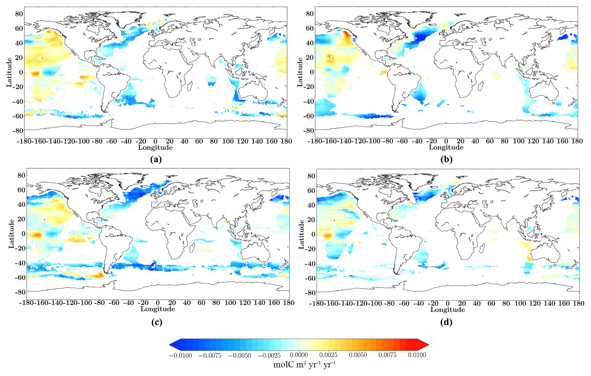
Figure 8 Significant (p_val =0.05) linear trend of fCO₂ for the common period (2001–2015) for (a) LSCE-FFNN, (b) Jena-MLS13, (c) ETH-SOMFFN and (d) JMA-MLR.

Table 3 Mean of sea–air CO₂ flux (PgC yr⁻¹) over the global ocean and per region for the common period (2001–2015). Averages over the period from 2001 to 2009 are presented in parentheses. The last column presents a comparison with the best estimates from Schuster et al. (2013) for the Atlantic Ocean (1990–2009).

Figure 8 shows the significant linear trends (p_val =0.05) of sea–air CO₂ fluxes for LSCE-FFNN (a), Jena-MLS13 (b), ETH-SOMFFN (c) and JMA-MLR (d). A total (averaged over the globe) negative trend was computed for all models, albeit with large regional contrasts, and LSCE-FFNN falls within this range: Jena-MLS13, −0.0012 PgC yr⁻¹ yr⁻¹ (−0.0028 PgC yr⁻¹ yr⁻¹, total value with no significant t test; Fig. S8); LSCE-FFNN, −0.00087 PgC yr⁻¹ yr⁻¹ (−0.0032 PgC yr⁻¹ yr⁻¹); JMA-MLR, −0.0013 PgC yr⁻¹ yr⁻¹ (−0.0037 PgC yr⁻¹ yr⁻¹); ETH-SOMFFN, −0.0025 PgC yr⁻¹ yr⁻¹ (−0.0059 PgC yr⁻¹ yr⁻¹). LSCE-FFNN computed negative trends over most of the Atlantic basin, the Indian Ocean and south of 40^∘ S, which contrasts with decreasing fluxes over the Pacific and locally in the Antarctic Circumpolar Current. At first order, this broad regional pattern is found in all models. However, regional maxima and minima are more pronounced in Jena-MLS13 (Fig. 8b) and ETH-SOMFFN (Fig. 8c), whereas a patchy distribution at the sub-basin scale is diagnosed for JMA-MLR.

The agreement in sign of computed linear trends from the four models is presented in Fig. 9 (total linear trends with no significant t test). Over most of the ocean, all four models show very close sea–air CO₂ tendency. In the Indian Ocean (biome 14), in comparison, a positive trend was computed for JMA-MLR (0.0004 PgC yr⁻¹ yr⁻¹; 0.00006 PgC yr⁻¹ yr⁻¹ with a t test), whereas the other three models present a negative trend. The differences between models were also found in the Pacific Ocean, especially the southern Pacific. In the eastern equatorial Pacific region (biome 6) a total significant negative trend is presented by all models. All models reproduced a maximum in the southern part of biome 6, but they disagreed about its amplitude and spatial distribution. Almost everywhere over the Atlantic Ocean the mapping methods produced the same sign of linear trend (Fig. 9). However, in the eastern part of the subtropical North Atlantic, Jena-MLS13 gave a positive linear trend of fCO₂ (Fig. 8b).

Figure 9 Agreement between the four mapping methods with respect to their linear trend of sea–air CO₂ flux. The color bar represents the number of products that have the same sign of linear trend.

According to LSCE-FFNN, the global ocean took up 1.55 PgC yr⁻¹ on average between 2001 and 2015.This estimate is consistent with results from the other three models (Table 3; see Table S2 for estimations per biome). The spread between individual models falls in the range of the error reported in Landschützer et al. (2016), ±0.4–0.6 PgC yr⁻¹. Per biome, estimates of CO₂ sea–air fluxes provided by LSCE-FFNN are also in good agreement with those derived from the other models.

4 Summary and conclusion

We proposed a new model for the reconstruction of monthly surface ocean pCO₂. The model is applied globally and allows a seamless reconstruction without introducing boundaries between the ocean basins or biomes. Our model relies on a two-step approach based on feed-forward neural networks (LSCE-FFNN). The first step corresponds to the reconstruction of a monthly pCO₂ climatology. It allows for the output of the FFNN to be kept close to the observed values in regions with poor data cover. In the second step, pCO₂ anomalies are reconstructed with respect to the climatology from the first step. The model was applied over the period from 2001 to 2016. Validation with independent data at the global scale indicated a RMSE of 17.57 µatm, an r² of ∼0.76 and an absolute bias of 11.52 µatm. In order to assess the model further, it was compared to three different mapping models: ETH-SOMFFN (self-organizing maps + neural network), Jena-MLS13 (statistical interpolation) and JMA-MLR (linear regression) (Rödenbeck et al., 2015). Network qualification followed the protocol and diagnostics proposed in Rödenbeck et al. (2015).

Reconstructed surface ocean pCO₂ distributions were in good agreement with other models and observations. The seasonal variability was reproduced to a satisfying level by LSCE-FFNN, the yearly pCO₂ mismatch varied around zero and the relative IAV mismatch was 7 %. LSCE-FFNN proved skillful in reproducing the interannual variability of surface ocean pCO₂ over the eastern equatorial Pacific in response to ENSO. Reductions in surface ocean pCO₂ during El Niño events were well reproduced. The comparison between reconstructed and observed pCO₂ values yielded a RMSE of 15.73 µatm, an r² of 0.79 and an absolute bias of 10.33 µatm over the equatorial Pacific. The relative IAV misfit in this region was ∼17 %. Despite the overall good agreement between models, important differences still exist at the regional scale, especially in the Southern Hemisphere and, in particular, in the southern Pacific and the Indian Ocean. These regions suffer from poor data coverage. Large regional uncertainties in reconstructed surface ocean pCO₂ and sea–air CO₂ fluxes have a strong influence on global estimates of CO₂ fluxes and trends.