CO₂ drawdown due to particle ballasting by glacial aeolian dust: an estimate based on the ocean carbon cycle model MPIOM/HAMOCC version 1.6.2p3

Despite intense efforts, the mechanisms that drive glacial–interglacial changes in atmospheric pCO₂ are not fully understood. Here, we aim at quantifying the potential contribution of aeolian dust deposition changes to the atmospheric pCO₂ drawdown during the Last Glacial Maximum (LGM). To this end, we use the Max Planck Institute Ocean Model (MPIOM) and the embedded Hamburg Ocean Carbon Cycle model (HAMOCC), including a new parameterization of particle ballasting that accounts for the acceleration of sinking organic soft tissue in the ocean by higher-density biogenic calcite and opal particles, as well as mineral dust. Sensitivity experiments with reconstructed LGM dust deposition rates indicate that the acceleration of detritus by mineral dust played a small role in atmospheric pCO₂ variations during glacial–interglacial cycles – on the order of 5 ppmv, compared to the reconstructed ∼80 ppmv rise in atmospheric pCO₂ during the last deglaciation. The additional effect of the LGM dust deposition, namely the enhanced fertilization by the iron that is associated with the glacial dust, likely played a more important role; although the full iron fertilization effect can not be estimated in the particular model version used here due to underestimated present-day non-diazotroph iron limitation, fertilization of diazotrophs in the tropical Pacific already leads to an atmospheric pCO₂ drawdown of around 10 ppmv.

1 Introduction

According to ice core data (Lüthi et al., 2008; Marcott et al., 2014; Köhler et al., 2017), the atmospheric CO₂ concentration during the Last Glacial Maximum (LGM, ∼ 21 000 years ago) was about 80 ppmv lower than during the early Holocene. Model simulations show that the reduced atmospheric CO₂ concentration caused a global cooling and, combined with orbital effects on Earth's climate, allowed the Laurentide, Cordilleran, British, and Scandinavian ice sheets to build up (Abe-Ouchi et al., 2007; Heinemann et al., 2014; Ganopolski and Brovkin, 2017). It is still a matter of active discussion, however, which of the many potential climate and carbon cycle changes in response to the orbital forcing caused how much of the atmospheric pCO₂ drawdown (e.g. Brovkin et al., 2012; Chikamoto et al., 2012; Ganopolski and Brovkin, 2017).

Here we introduce a new parameterization of the effect of higher-density particles such as calcite, opal, and dust on the sinking speed of detritus into the Max Planck Institute Ocean Model (MPIOM) with the embedded Hamburg Ocean Carbon Cycle model (HAMOCC). Based on this new model set-up, we estimate to what extent enhanced aeolian dust deposition contributed to the reconstructed atmospheric pCO₂ drawdown during the last glacial period due to its effect on particle ballasting.

Observationally constrained simulations of the global dust cycle have suggested that dust production and deposition rates were at least twice as large during the LGM compared to the Holocene and present due to (1) enhanced desert dust production and (2) enhanced glacigenic dust production (e.g. Werner et al., 2002; Mahowald et al., 2006; Albani et al., 2016). The increased desert dust production was caused mainly by a reduction in terrestrial vegetation (leading to larger desert dust source areas) due to inverse CO₂ fertilization, temperature, precipitation, and cloudiness changes (Mahowald et al., 2006) or by stronger tropospheric winds (Werner et al., 2002). Glacigenic dust, which is produced by the grinding of ice sheets and glaciers over the bedrock and sediments, and the subsequent transport by meltwater beyond the ice margin of the fine sediment produced (e.g. Bullard, 2013), contributed to the enhanced dust deposition, and, globally, the magnitude of this glacigenic dust contribution was comparable to that of desert dust (Mahowald et al., 2006).

It is well known that enhanced glacigenic and desert dust deposition in particular over the Southern Ocean can strengthen the biological carbon pump due to fertilization with the bioavailable iron contained in the dust (Martin, 1990; Kumar et al., 1995; Sigman and Boyle, 2000; Werner et al., 2002). This iron hypothesis is supported for example by mesoscale iron enrichment experiments which demonstrated that primary production in one third of the world ocean is limited by iron availability (Boyd et al., 2007). Various modelling studies testing this classical iron hypothesis have concluded that a range of 15–40 ppmv of the reconstructed 80 ppmv atmospheric pCO₂ difference can be explained by iron fertilization due to dust deposition changes (Watson et al., 2000; Bopp et al., 2003; Brovkin et al., 2007; Hain et al., 2010; Lambert et al., 2015; Ganopolski and Brovkin, 2017). Moreover, it has been suggested that the enhanced LGM dust deposition led to a fertilization of nitrogen fixation (diazotrophy, e.g. of the dominant nitrogen-fixing cyanobacteria Trichodesmium) in the Pacific, potentially leading to an additional uptake of CO₂ from the atmosphere by the ocean (Moore and Doney, 2007).

Enhanced dust deposition can also have an effect on the sinking speed and remineralization length scale of particulate organic carbon (POC or detritus). Detritus sinks because of its higher density compared to seawater (excess density). As aggregates including POC form, ballast minerals, i.e. silicate and calcite biominerals, as well as lithogenic minerals such as aeolian dust, which are denser than organic tissue and seawater, provide a major weight fraction of sinking particles in the deep ocean (Honjo et al., 1982). Hence, ballast minerals contribute largely to the excess density of aggregates including detritus in the deep ocean. This led to the hypothesis that ballast minerals determine accelerated deep-water POC fluxes (ballasting hypothesis; e.g. Armstrong et al., 2002). Several deep-moored sediment trap observations of particle flux rates supported this ballasting hypothesis (see Boyd and Trull, 2007, for a review). While Klaas and Archer (2002) and François et al. (2002), for example, confirmed the association of calcite minerals with efficient transfer of POC to the deep ocean but suggested that the role of lithogenic minerals is negligible (see also Berelson, 2001), Dunne et al. (2007) suggested that neglecting lithogenic material in carbon cycle models would lead to an underestimation of the POC flux to the seafloor by 16 %–51 % globally. Noticeably high sinking speeds off northwest Africa (Fischer and Karakaş, 2009) and artificial dust deposition experiments using natural plankton communities from off Mauritania and Saharan dust (van der Jagt et al., 2018) further support the hypothesis that dust deposition can accelerate the sinking of detritus.

Still, to the best of our knowledge, the hypothesis that particle ballasting changes due to variations in fluxes of lithogenic material into the ocean contributed to the reconstructed atmospheric pCO₂ changes during glacial–interglacial cycles (Ittekkot, 1993) has not yet been tested using ocean–biogeochemical models.

This paper is organized as follows. In Sect. 2, we describe our configuration of the ocean circulation and carbon cycle model MPIOM/HAMOCC (Sect. 2.1), introduce a simple particle ballasting scheme that includes the effect of lithogenic minerals from aeolian sources (Sect. 2.2), and describe the spin-up procedure of the model (Sect. 2.3). In Sect. 3, we describe the necessary adjustment of HAMOCC parameters to the modified sinking speeds (Sect. 3.1) and compare the resulting reference simulation with the new particle ballasting to a reference simulation with the standard prescribed particle sinking speeds and to observations (Sect. 3.2). In Sect. 4, sensitivity experiments with respect to LGM instead of modern dust deposition rates are presented to estimate the role of particle ballasting changes for glacial–interglacial atmospheric pCO₂ changes. Since the dust deposition fields are also used to compute the concentrations of bioavailable iron in HAMOCC, the LGM dust deposition changes have two effects, enhanced particle ballasting and iron fertilization. We isolate these two effects from each other but will also show that the iron fertilization effect in the particular model version used in this study underestimates the observed present-day iron limitation in the Southern Ocean, likely leading to an underestimation of the iron fertilization effect of enhanced LGM dust deposition. We conclude with a summary and discussion of our results (Sect. 5).

2 Methods

To quantify the effect of aeolian dust variations on atmospheric pCO₂, we use MPIOM and the embedded HAMOCC (Sect. 2.1). To account for particle ballasting effects, the default prescribed Martin-type sinking for detritus and the constant sinking speeds for opal, dust, and calcite are replaced by a simple prognostic particle ballasting parameterization following Gehlen et al. (2006), which assumes that detritus and the denser particles form aggregates that sink at speeds computed from the density differences between these imaginary aggregates and the surrounding seawater (Sect. 2.2). The particle ballasting parameterization derived here following Gehlen et al. (2006) differs for example from another approach that assumes that only a fraction of POC is sinking in association with ballast (e.g. Klaas and Archer, 2002; Armstrong et al., 2002; Howard et al., 2006; Hofmann and Schellnhuber, 2009). Note that the particle ballasting parameterization is, implicitly, also the very simplest aggregation model possible – assuming that all particulate matter instantly forms homogeneous aggregates, neglecting the complex biological and physical aggregation and disaggregation processes that occur in reality (e.g. Lam and Marchal, 2015) or that are explicitly captured in more complex (and computationally more expensive) aggregation models (e.g. Kriest and Evans, 2000).

Using the new particle ballasting parameterization, we then perform sensitivity tests to quantify the effect of dust deposition changes on the atmosphere–ocean CO₂ fluxes, separating the effects of (1) particle ballasting by the dust and (2) fertilization by the bioavailable iron associated with the dust. The presented sensitivity tests are simulations with prescribed modern or LGM dust deposition fields, atmospheric climatological forcing representing modern conditions, and pre-industrial greenhouse gas concentrations (GHGs). The atmosphere–ocean CO₂ flux anomalies in the simulations with LGM dust are used to estimate the effect of dust changes on atmospheric pCO₂ variations during glacial cycles. We do not perform transient simulations of glacial cycles yet because (1) dust deposition fields are currently only available for snapshots during the last deglaciation and (2) the computational cost and required wall time to transiently simulate a glacial cycle or inception is currently too large.

2.1 Configuration of MPIOM/HAMOCC

Our results are based on the ocean-only model configuration of the Max Planck Institute Earth System Model (MPI-ESM; Giorgetta et al., 2013) version 1.2.00p4, which contains MPIOM version 1.6.2p3 (corresponding to revision 3997). MPI-ESM is a comprehensive Earth system model that consists of the atmosphere general circulation model ECHAM (Stevens et al., 2013), the land surface scheme JSBACH (Raddatz et al., 2007), and the ocean circulation model MPIOM (Jungclaus et al., 2013), which contains the ocean biogeochemistry model HAMOCC (Ilyina et al., 2013; Paulsen et al., 2017) including a sediment module (Heinze et al., 1999). MPI-ESM has been used successfully for millennial-scale atmosphere–ocean–carbon cycle simulations, including a transient simulation of the last millennium with fully interactive atmospheric CO₂ (Jungclaus et al., 2010). Since our aim is to isolate the effect of particle ballasting changes in the ocean during glacial–interglacial cycles on the atmosphere–ocean CO₂ fluxes, rather than realistically simulating past climate evolution, we use the ocean–only configuration of MPI-ESM, namely MPIOM/HAMOCC in a stand-alone mode (Marsland et al., 2003; Maier-Reimer et al., 2005; Paulsen et al., 2017).

However, for the sensitivity experiments with LGM dust deposition fields, we do consider variable atmospheric pCO₂ with a simple atmospheric CO₂ box model based on atmosphere–ocean CO₂ flux anomalies relative to a reference simulation with modern dust deposition and ballasting (PI_BALLAST). The flux anomalies are diagnosed at the end of each simulated year, and the prescribed atmospheric pCO₂ is updated accordingly. For an accumulated net atmosphere–ocean CO₂ flux anomaly of 2.1 Gt C into the ocean, the atmospheric CO₂ concentration is reduced by 1 ppmv. Note that only the surface ocean biogeochemistry responds to this atmospheric pCO₂ feedback. There is no effect on the atmospheric radiative transfer or climate; the prescribed climatological atmospheric forcing is unchanged. If the atmospheric CO₂ concentration was not adjusted to the flux anomalies, for example, a positive anomalous ocean CO₂ uptake would not result in a reduced atmospheric pCO₂, the atmosphere would behave like a CO₂ reservoir in our experiments, and the subsequent ocean CO₂ uptake would be overestimated (as illustrated by an additional experiment in Sect. 4.1 with LGM dust deposition for particle ballasting but without adjusting atmospheric pCO₂, shown as a blue dashed line in Fig. 5b). The long-term net ocean CO₂ uptake in our reference simulations (Fig. 5b) would lead to a negative CO₂ trend if absolute atmosphere–ocean CO₂ fluxes were used; we avoid this effect by computing atmospheric CO₂ from the flux anomalies relative to the reference simulation in each year. Moreover, this approach of computing flux anomalies each year, compared to, e.g., the alternative of subtracting the mean reference run flux imbalance, avoids additional atmospheric pCO₂ variability due to, e.g., internal variability of the ocean circulation. By using this simple atmospheric pCO₂ box model in combination with MPIOM/HAMOCC rather than using the coupled MPI-ESM, atmosphere and land surface feedbacks to the pCO₂ variations – that would alter the ocean circulation and complicate the analysis of dust-related CO₂ flux anomalies – are avoided and computational time is saved.

Another measure to save computational time is the use of a relatively coarse predefined, bipolar, curvilinear ocean grid (GR30L40) with a grid-point spacing of ∼3^∘ and 40 levels, with thicknesses ranging from 10–12 m in the upper ocean to 600 m in the deepest ocean.

The ocean model MPIOM is forced by a repeating 1-year-long climatology of daily mean surface boundary conditions, including 2 m air temperature, zonal and meridional wind stress, wind speed, shortwave radiation, total cloud cover, precipitation, and river runoff, representing modern conditions based on the ERA40 and ERA15 reanalyses (Röske, 2005, 2006) as in Paulsen et al. (2017).

To avoid salinity trends due to imbalances in precipitation, evaporation, and river runoff, the surface salinity is restored with a relaxation coefficient of $\mathrm{3.3}\times {\mathrm{10}}^{-\mathrm{7}}$ s⁻¹ to the annual salinity field of the Polar science center Hydrographic Climatology (PHC).

Note that biogeochemical changes do not affect the ocean circulation in the default (and our) configuration of MPIOM/HAMOCC. That means, for example, that any effect of phytoplankton concentration changes on light absorption (Wetzel et al., 2006) is neglected in MPIOM. Differences in the ocean circulation between our simulations with the standard MPIOM/HAMOCC set-up and the set-up that includes particle ballasting are only due to the fact that, unfortunately, different numbers of CPUs were used for the computations (Fig. 1a: black line covers the coloured lines, but not the dark grey line of the set-up without ballasting). For binary-identical results, the parameter “nprocx” must not be changed. Otherwise, the spatial and temporal variations in the ocean circulation would be identical in the spin-up with the standard model and the simulations with ballasting.

2.2 Particle sinking and ballasting in HAMOCC

In the standard version of HAMOCC, particle ballasting is not accounted for. Calcite and opal shells sink at a prescribed, constant speed of 30 m d⁻¹; dust sinks at a speed of only 0.05 m d⁻¹, resulting from the assumption of spherical dust particles with a diameter of 1 µm following Stokes' law (Stokes' drag is balanced by gravitational force minus buoyancy force); the sinking speed of detritus w_det is constant in the euphotic zone and increases with depth z below the euphotic zone (z>100 m) following Martin et al. (1987):

$$\begin{array}{}\text{(1)}& w_{\det }\left(z\right)=w_{\mathrm{eu}}+\left\{\begin{array}{ll}\mathrm{0},& z\le \mathrm{100}\mathrm{m}\\ \frac{{\mathit{\lambda }}_{\det }}{b}(z-\mathrm{100}\mathrm{m}),& z>\mathrm{100}\mathrm{m},\end{array}\right.\end{array}$$

where w_eu=3.5 m d⁻¹ is the sinking speed in the euphotic zone, the parameter b is set to 2, and the remineralization rate for detritus λ_det is set to 0.026 d⁻¹, resulting in sinking speeds of up to 80 m d⁻¹ (Fig. 2b).

To account for particle ballasting, we add a simple parameterization of particle sinking speeds to HAMOCC. We assume that all particulate matter forms aggregates and sinks together at a common speed w_ballast. As suggested by Gehlen et al. (2006), the common speed is proportional to the difference between the mean density of all particles ρ_particles and the density of the seawater ρ_sw in each model grid box:

$$\begin{array}{}\text{(2)}& w_{\mathrm{ballast}}=w_{\mathrm{0}}\cdot {\displaystyle \frac{{\mathit{\rho }}_{\mathrm{particles}}-{\mathit{\rho }}_{\mathrm{sw}}}{{\mathit{\rho }}_{\det }-{\mathit{\rho }}_{\mathrm{sw}}}}.\end{array}$$

w₀ is the proportionality factor and can be interpreted as the sinking speed of the aggregate in the absence of particle ballast. The density difference ρ_particles−ρ_sw is also called excess density. The mean density of all particles ρ_particles is given by the mass of all particles per unit volume of seawater, divided by the volume of all particles per unit volume of seawater. In contrast to Gehlen et al. (2006), here, dust also contributes to the ballasting of detritus:

$$\begin{array}{}\text{(3)}& {\mathit{\rho }}_{\mathrm{particles}}={\displaystyle \frac{c_{\mathrm{dust}}+{\sum }_b{m}_b{\mathrm{\Psi }}_b}{\frac{\mathrm{1}}{{\mathit{\rho }}_{\mathrm{dust}}}{c}_{\mathrm{dust}}+{\sum }_b\frac{m_b}{{\mathit{\rho }}_b}{\mathrm{\Psi }}_b}},\end{array}$$

where c_dust is the mass concentration of dust (mass of dust per unit volume of seawater, in g cm⁻³), ρ_dust is the density of dust (2.50 g cm⁻³), Ψ_b is the molar concentration of the biogenic particle types b (namely: detritus, calcite, and opal, in mol C and mol Si cm⁻³, respectively), m_b is their molar mass (32.7 g (mol C)⁻¹ for detritus, 100.0 g (mol C)⁻¹ for calcite, and 72.8 g (mol Si)⁻¹ for opal), and ρ_b is their density (1.06 g cm⁻³ for detritus, 2.71 g cm⁻³ for calcite, and 2.10 g cm⁻³ for opal).

Monthly mean dust deposition rates are prescribed based on numerical reconstructions of modern and LGM boundary conditions, including glacigenic dust (Fig. 6a–b; Mahowald et al., 2006). The dust deposition fields not only affect the sinking speed in our ballasting parameterization, but also the availability of iron. It is assumed that 3.5 % (weight) of the dust in the water column is iron, of which 1 % is soluble and bioavailable.

2.3 Spin-up of the standard model set-up

Before starting our experiments with particle ballasting, we spin up the standard version of MPIOM/HAMOCC without particle ballasting for over 10 000 years (Fig. 1). During the spin-up phase, the ocean model, which is initialized from three-dimensional PHC temperature and salinity fields, approaches an equilibrium state (thanks to the salinity restoration at the surface). The simulated ocean circulation is characterized by deep-water formation in the Atlantic and Southern oceans, and no deep-water formation in the Pacific; the Atlantic meridional overturning at 26^∘ N amounts to about 17 Sv (sverdrup; 10⁶ m³ s⁻¹; Fig. 1a).

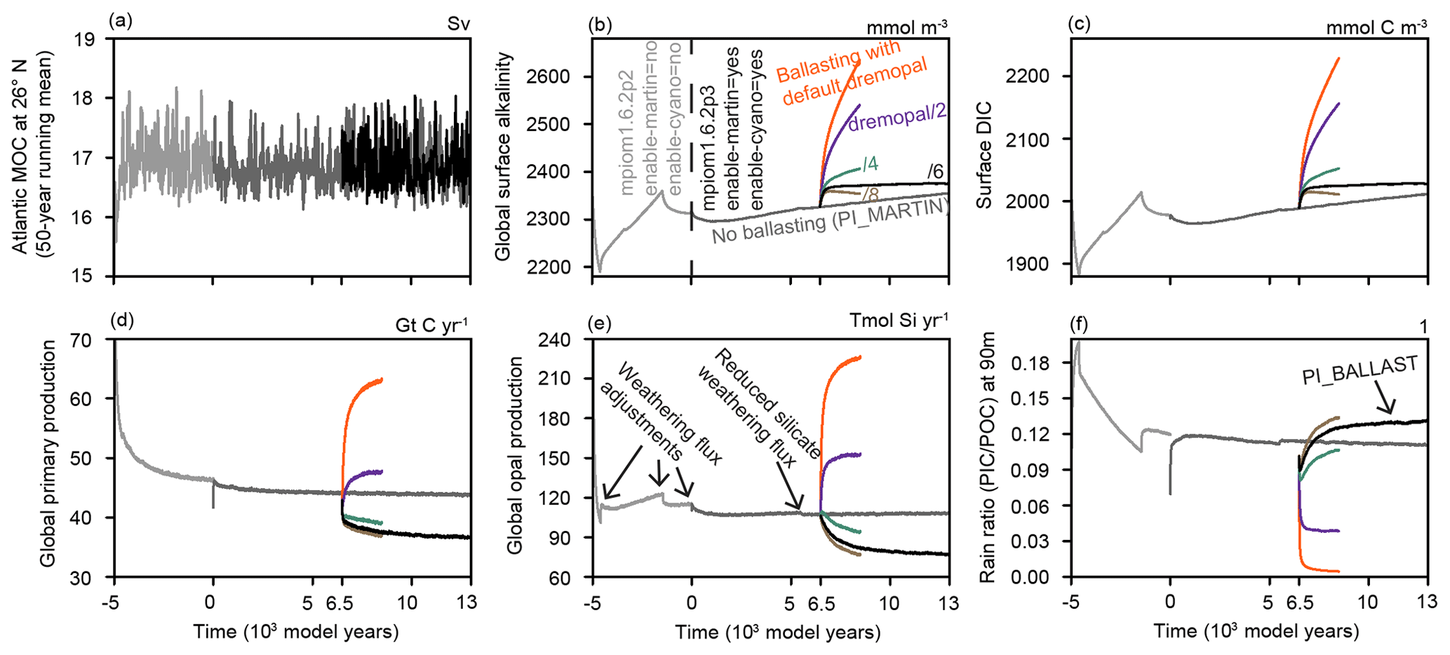
Figure 1 Selection of the weathering rates during the spin-up of MPIOM/HAMOCC and adjustment of the opal remineralization rate to modified sinking speeds. (a) Strength of the Atlantic Meridional Overturning Circulation (AMOC) at 26^∘ N; (b) surface alkalinity; (c) surface dissolved inorganic carbon (DIC); (d) global primary production; (e) global opal production; and (f) ratio of global calcite to organic carbon export at 90 m depth (rain ratio). The initial 5000-year long simulation was done with an older MPIOM/HAMOCC set-up; we do not intend to interpret the biogeochemistry of this run. However, the endpoint of this older simulation is used as a starting point for our modern control simulation without particle ballasting, using the default-configuration of MPIOM/HAMOCC in MPI-ESM 1.2.00p4, including a new parameterization of diazotrophs (Paulsen et al., 2017) and Martin-type sinking (darker grey). In model year 6500, the ballasting parameterization is switched on, and, to compensate for the reduced sinking speed of opal in the euphotic zone, the opal dissolution rate λ_opal (namelist parameter dremopal) is reduced from 0.01 d⁻¹ by factors of 2, 4, 6, and 8.

The ocean carbon cycle is not so easily tamed, since it remains an open system in our model (no restoring). To reach a stable equilibrium of the carbon cycle in the water column and the sediment, the net fluxes of organic carbon, calcite, and opal from the ocean column to the sediment – which are computed in HAMOCC – need to be balanced by the fluxes into the ocean of organic matter, calcite, and silicate from weathering on land – which are prescribed as namelist parameters (called deltaorg, deltacal, and deltasil). The weathering fluxes are adjusted several times during the spin-up phase, aimed at (1) balancing the sediment burial fluxes as diagnosed from the trends in the sediment inventory over several hundred years prior to each weathering flux adjustment, (2) a stable calcite export production at 90 m depth of about 1 Gt C yr⁻¹, and (3) a rain ratio (ratio of calcite export to detritus export at 90 m depth) of about 10 % (Fig. 1f). An equilibrium of the sediment, however, is not reached in our simulations. Note that the selection of the weathering fluxes itself affects the simulated biogeochemistry. For example, if the silicate weathering flux is increased, more opal can be produced, and calcite production is suppressed (see Eqs. 12–14 of Ilyina et al., 2013).

3 Results for modern dust deposition

To simulate a reasonably realistic carbon cycle with atmosphere–ocean CO₂ fluxes comparable to observations and to create a mean state with particle ballasting that is very close to the mean state of the standard set-up, it is important to adjust HAMOCC to the substantially modified particle sinking speeds that result from the particle ballasting parameterization. In this section, we argue that this adjustment can be achieved by a reduction in the opal dissolution rate (Sect. 3.1) and then compare the resulting carbon cycle simulation with particle ballasting (PI_BALLAST) to the simulation with the standard prescribed or Martin-type POC sinking (PI_MARTIN) and to observational data (Sect. 3.2).

3.1 Adjusting HAMOCC to the new particle sinking

The simulations with particle ballasting are initialized from year 6500 of the reference simulation without particle ballasting (PI_MARTIN; Fig. 1b). Using a no-ballast reference speed w₀ (Eq. 2) of 0.5 m d⁻¹ leads to global mean sinking speeds w_ballast of the virtual aggregates between about 5 m d⁻¹ at the surface and about 120 m d⁻¹ below 5 km depth (Fig. 2b). A larger w₀, such as 3.5 m d⁻¹ as used by Gehlen et al. (2006), would lead to much higher global mean sinking speeds. The advantage of using the small w₀ is that it yields global mean aggregate sinking speeds that are comparable to the depth-dependent, Martin-type sinking speed of detritus that is prescribed in PI_MARTIN (Fig. 2b) and to a similar POC flux profile (Fig. 2a), which allows us to avoid a re-tuning of the remineralization rate of detritus.

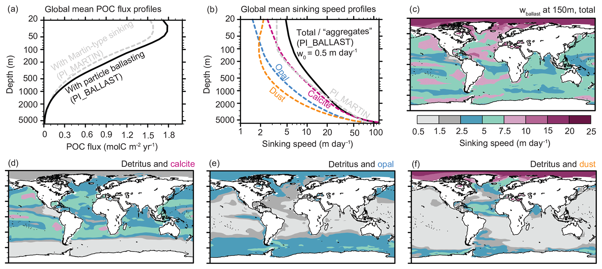
Figure 2 Global mean particulate organic carbon (POC) flux profiles (a) and particle sinking speed w_ballast for (b) global mean profiles and (c–f) at 150 m depth. The contributions of the different ballast types (calcite, opal, and dust) to the resulting, applied “aggregate” sinking speed (black) are estimated by recomputing the sinking speed assuming that only one type of ballast is present. The dashed grey line in panel (a) shows the Martin-type sinking speed applied to POC in every water column in the reference simulation without ballasting (PI_MARTIN). Note the logarithmic depth scale.

The dissolution rate of opal, however, needs to be re-tuned, since the sinking speed of opal is reduced from previously 30 m d⁻¹ to now only ∼5 m d⁻¹ in the euphotic zone (Fig. 2b). Consequently, more opal is dissolved within the euphotic zone, leading to higher silicate concentrations, a higher opal production rate (Fig. 1e), and a very low rain ratio (Fig. 1f) due to a completely suppressed calcite production. Without adjusting the river input (weathering) of calcite to the reduced calcite precipitation and burial, surface alkalinity and dissolved inorganic carbon (DIC) rise (Fig. 1b–c). For a reduction in the opal dissolution rate by a factor of 6, the trends in alkalinity and DIC become small and comparable to (or actually smaller than) the trend in the control simulation without ballasting (Fig. 1b–c), and, even without readjusting the weathering fluxes, a stable carbon cycle simulation with particle ballasting (PI_BALLAST) is achieved that is similar to PI_MARTIN.

3.2 Ballasting effects and comparison to observations

For pre-industrial GHGs (pCO₂=278 ppmv), modern ocean circulation, and modern dust deposition (Fig. 6a), the simulated atmosphere–ocean CO₂ fluxes in the standard set-up (PI_MARTIN) and the set-up with particle ballasting (PI_BALLAST) are hardly distinguishable (Fig. 3b–c). There are, however, clear differences compared to the observed modern CO₂ fluxes (Fig. 3a). Most notably, the observed flux of CO₂ from the atmosphere into the ocean between 30 and 60^∘ S in the South Atlantic, Indian Ocean, and west Pacific is underestimated, due to an overestimation of the ocean surface pCO₂, as previously reported for HAMOCC within the coupled MPI-ESM (Ilyina et al., 2013). Also note that the CO₂ flux data (Takahashi et al., 2009) are based on modern observations, while pre-industrial GHGs are prescribed in the model simulations.

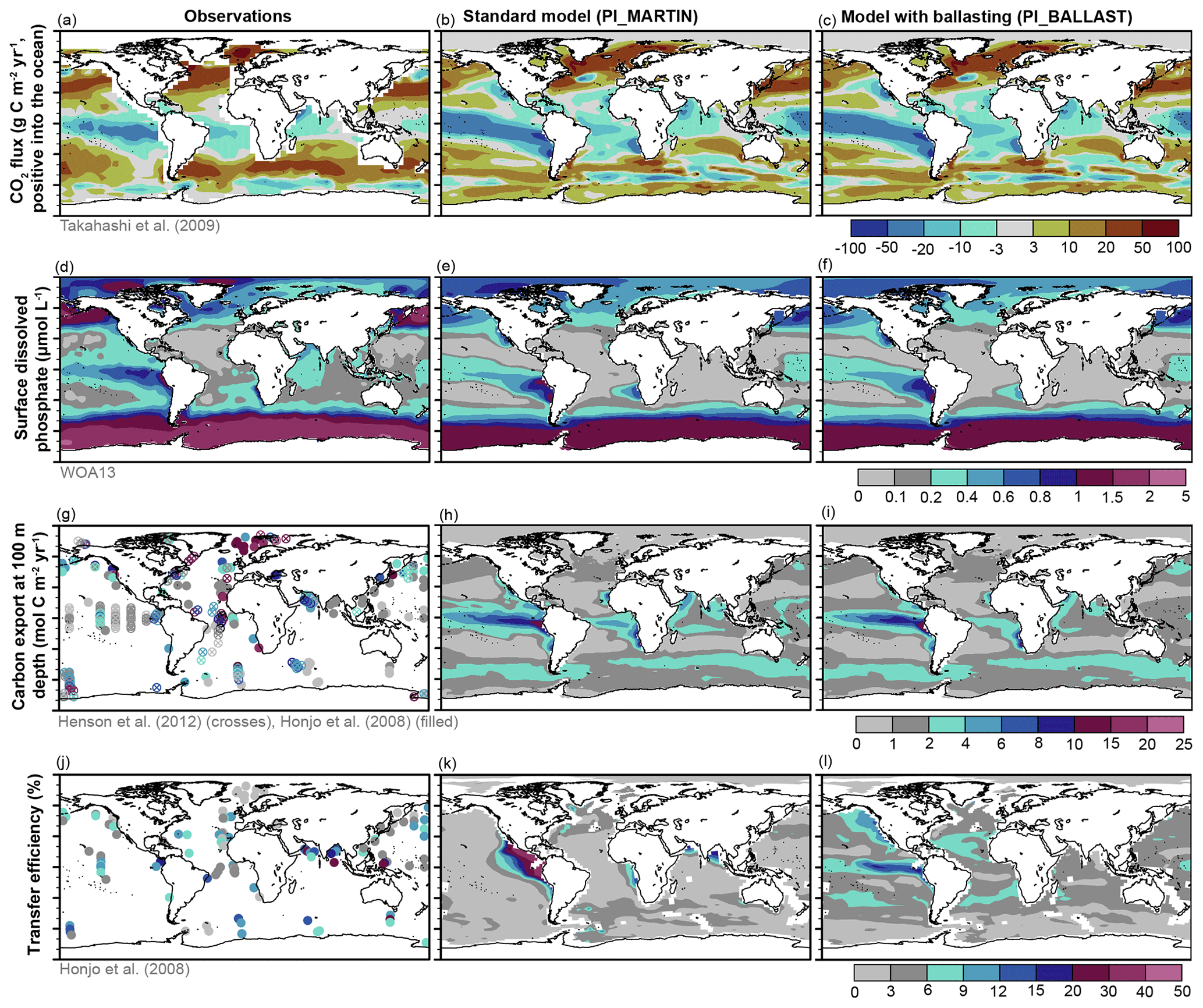
Figure 3 Comparison of the reference simulations with particle ballasting (PI_BALLAST) and without particle ballasting (standard set-up with constant or Martin-type particle sinking; PI_MARTIN) to observations. (a–c) Net atmosphere-to-ocean CO₂ flux from observations (Takahashi et al., 2009) compared to our simulations; (d–f) surface dissolved phosphate from the World Ocean Atlas (Garcia et al., 2013) compared to our simulations; (g–i) carbon export at 100 m depth as derived from satellite data (Henson et al., 2012; crosses) and from sediment trap data (Honjo et al., 2008; filled circles) compared to the export at 90 m depth in our simulations; and (j–l) transfer efficiency (carbon flux at 2000 m depth divided by the carbon flux at 100 m depth) as derived from sediment trap data (Honjo et al., 2008) compared to the 90 to 2080 m transfer efficiency in our simulations. For all simulations in this figure, modern dust deposition rates were prescribed; shown are averages computed over the model years 12 900 to 12 999.

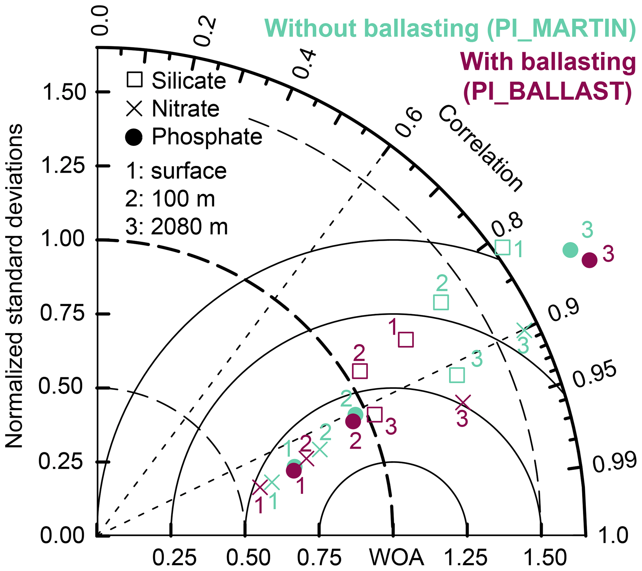
Figure 4 Taylor diagram comparing annual mean silicate (squares), nitrate (crosses), and phosphate concentrations (dots) at three different depths (numbers) of the pre-industrial reference simulations with Martin-type sinking (PI_MARTIN, aquamarine) and with particle ballasting (PI_BALLAST, pink) to World Ocean Atlas data (WOA; Garcia et al., 2013).

A comparison of simulated to observed nutrient concentrations is shown in Fig. 3d–f for phosphate at the surface and in a Taylor diagram (Fig. 4) at the surface, 100 m depth, and 2 km depth for phosphate, nitrate, and silicate. The surface dissolved phosphate concentrations are hardly distinguishable in the simulations with particle ballasting (PI_BALLAST) and without particle ballasting (PI_MARTIN). Compared to World Ocean Atlas data (WOA; Garcia et al., 2013), the simulated phosphate concentrations in the Southern Ocean, Indian Ocean, equatorial Pacific, and the North Pacific are underestimated (Fig. 3d–f), and these biases are again similar to previous HAMOCC studies (Ilyina et al., 2013). This similarity between the simulated phosphate concentrations is not only true at the surface, but also at depth (Fig. 4). The large overestimation of the spatial variability of the phosphate concentrations at 2 km depth in both simulations is due to an underestimation of the concentrations in the Atlantic and an overestimation in the eastern tropical Pacific (not shown). For nitrate, the observed high concentrations in the Antarctic circumpolar region at the surface and 100 m depth are underestimated in both simulations, leading to an underestimated spatial variability at these depths (Fig. 4). At 2 km depth, the simulation with particle ballasting fits better to observations (Fig. 4), especially due to an improved fit in the eastern Pacific (nitrate concentrations are overestimated in the eastern Pacific in PI_MARTIN, while they fit relatively well in PI_BALLAST; not shown). For silicate concentrations, the fit to observations is improved at the surface and at 100 m depth in the simulation with particle ballasting, mostly because the concentrations in the Antarctic circumpolar region match observations well in PI_BALLAST, while they are overestimated in PI_MARTIN. At 2 km depth, the fit is also improved in PI_BALLAST due to a reduction in the positive concentration bias in the eastern Pacific (compared to PI_MARTIN).

The global primary production in the simulation with ballasting amounts to about 39 Gt C yr⁻¹ compared to 44 Gt C yr⁻¹ in the simulation without particle ballasting (Fig. 1d), not including the primary production by diazotrophs, which amounts to additional 5 and 4 Gt C yr⁻¹ for PI_BALLAST and PI_MARTIN, respectively. The global organic matter export is slightly reduced (7.0 Gt C yr⁻¹ compared to 7.5 Gt C yr⁻¹ without ballasting), and the global calcite production and export are only moderately larger (1 Gt C yr⁻¹ compared to 0.85 Gt C yr⁻¹ without ballasting, not shown), leading to an elevated rain ratio of about 13 % compared to 11 % in the simulation without ballasting (Fig. 1f). Opal production (Fig. 1e) and opal export at 90 m (not shown) are reduced by about 30 % in the simulation with modern dust and ballasting compared to the run without ballasting (production: 76 versus 108 Tmol Si yr⁻¹; export: 72 versus 103 Tmol Si yr⁻¹).

The simulated spatial pattern of the carbon export at 90 m depth (export production) in PI_MARTIN and PI_BALLAST are very similar to each other, with the area of high export production in the equatorial Pacific extending further into the subtropics in PI_MARTIN (Fig. 3h–i). Compared to estimates based on sediment trap data (Honjo et al., 2008) and satellite data (Henson et al., 2012), the simulated export production in both simulations is underestimated in the North Atlantic and overestimated in the equatorial Pacific (Fig. 3g–i).

Only a fraction of this export production from the euphotic zone reaches the deep ocean. This fraction, also called transfer efficiency, is a measure for the efficiency of the biological pump. The range of simulated transfer efficiencies through the mesopelagic zone (here computed as the simulated POC flux at 2080 m depth divided by the POC flux at 90 m depth in PI_BALLAST and PI_MARTIN) compares well with the range of transfer efficiency estimates based on sediment trap data (Honjo et al., 2008; Fig. 3j–l). In the simulation without particle ballasting (PI_MARTIN), the same sinking speed profile for POC is prescribed everywhere. Hence, the variations in the transfer efficiency are only due to local differences in the organic matter remineralization rate, which depends on oxygen availability. Denitrification and sulfate reduction remineralization rates combined are lower than aerobic remineralization rates (see Eq. 6 of Ilyina et al., 2013), leading to higher transfer efficiencies in oxygen minimum zones (OMZs), e.g. in the eastern equatorial Pacific, Arabian Sea, and Bay of Bengal (Fig. 3k). In the simulation with particle ballasting (PI_BALLAST), this effect of lower remineralization rates in OMZs is at least partly compensated for by reduced ballasting by calcite due to the corrosive waters, resulting in lower settling speeds and transfer efficiencies (Fig. 3l). The relatively high transfer efficiencies in the midlatitudes in PI_BALLAST compared to PI_MARTIN are in line with high particle sinking speeds mostly due to ballasting by calcite particles (compare Fig. 2d to Fig. 3l).

However, as far as we understand, even qualitatively, the global pattern of transfer efficiencies is uncertain: on the one hand, Henson et al. (2012) suggested that, based on satellite data, in large areas of the tropics and subtropics except in the eastern equatorial Pacific cold tongue, over 30 % of the export production at 100 m depth reach the deep ocean below 2000 m, while at high latitudes (>50^∘) less than 10 % of the export production reaches that depth. On the other hand, from nutrient distributions Weber et al. (2016) reconstructed a “global pattern of transfer efficiency to 1000 m that is high (∼25 %) at high latitudes and low (∼5 %) in subtropical gyres, with intermediate values in the tropics”.

Dust substantially affects sinking speeds and the transfer efficiencies in the Southern Ocean and South Atlantic off Patagonia, as well as in the equatorial Atlantic due to Saharan dust deposition, in the North Atlantic, and in the Arctic Ocean. Note, however, that, in particular in the Arctic Ocean, where POC concentrations are low, even small quantities of dust can lead to high sinking speeds (Fig. 2c and f), since our simple particle ballasting parameterization only takes into account the density of the dust (for POC concentrations tending to zero), and not its diameter. This leads to high sinking speeds in the model, while in reality, when POC concentrations are so low that particle collisions and aggregate formation are unlikely, the small and mostly individual dust particles sink very slowly according to Stoke's law. While this illustrates a limitation of the simple particle ballasting parameterization, the effect of the erroneously high sinking speeds in the Arctic on the carbon export is small: the integrated carbon export at 90 m depth north of 80^∘ N amounts to only 0.01 Gt C yr⁻¹ or just over 0.1 % of the global export of about 7 Gt C yr⁻¹.

In summary, although the simulated sinking speeds substantially differ between the simulations with and without particle ballasting, the biases of the set-up with particle ballasting compared to observations remain similar to the biases of the standard set-up. But the set-up with particle ballasting now enables us to estimate the effect of glacial dust deposition on atmospheric pCO₂.

4 Sensitivity to LGM dust deposition

Starting from the simulation with particle ballasting described in the previous section (PI_BALLAST, with the opal dissolution rate reduced by a factor of 6, modern dust deposition, modern ocean circulation, and pre-industrial GHGs), three experiments are performed to estimate the sensitivity of the ocean carbon cycle to the reconstructed LGM dust deposition. In all three sensitivity experiments, the prescribed monthly-mean modern dust deposition fields are replaced instantaneously by monthly-mean LGM dust deposition fields (see Fig. 5 for time series of the sensitivity experiments and Fig. 6a–c for maps of the annual mean dust deposition rates and the LGM–modern dust deposition difference). In the first experiment, the LGM dust deposition rates are only used for the computation of dust concentrations in the water column, isolating the ballasting effect of the LGM dust deposition (LGM_BALL; solid blue lines in Fig. 5). In the second experiment, the LGM dust deposition rates are only used for the computation of the bioavailable iron concentrations, isolating the iron fertilization effect associated with the dust (LGM_IRON; orange lines). In the third experiment, the LGM dust deposition is used for both particle ballasting and iron fertilization (LGM_BOTH; pink lines). Note that Fig. 5b depicts only the first 500 years of the experiments to illustrate the magnitude of the interannual to centennial variability compared to the dust effects, while panels (c)–(f) of Fig. 5 show the longer-term evolution of the induced anomalies over the entire 6500 years of the sensitivity experiments. The maps shown in Fig. 6d–l are computed from the first 100 years of the sensitivity experiments to capture the time of the largest atmosphere–ocean CO₂ flux anomaly signal.

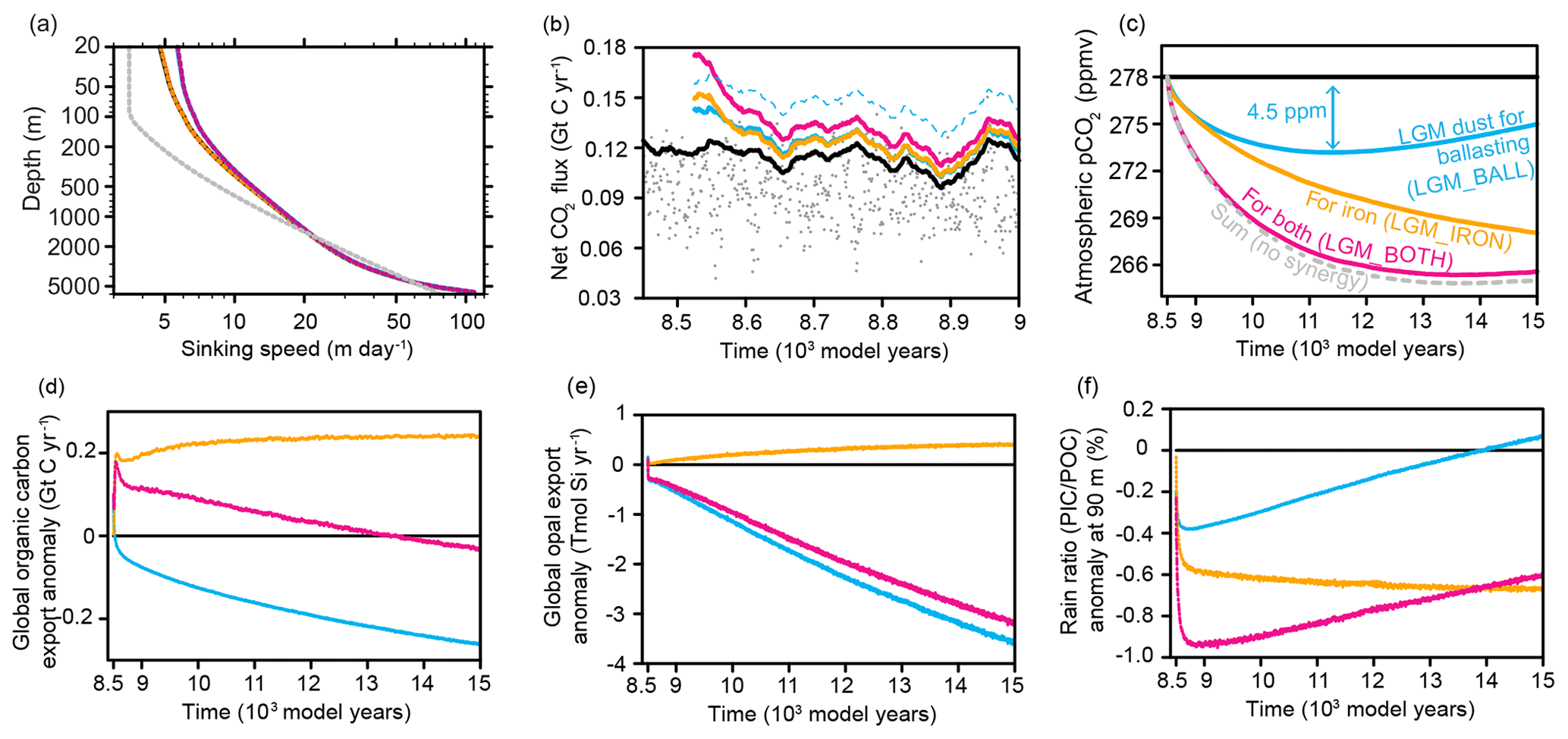
Figure 5 Effects of switching to LGM dust deposition for particle ballasting (LGM_BALL, blue), for the computation of iron fertilization associated with the dust (LGM_IRON, orange), and for both (LGM_BOTH, pink) compared to the control simulation with ballasting and iron fertilization based on modern dust deposition (PI_BALLAST, black). (a) Global mean sinking speed profiles; grey dashed line indicates the Martin-type sinking speed profile as used in the standard simulation without ballasting (PI_MARTIN); note that the black curve (PI_BALLAST) is hidden behind the orange curve (LGM_IRON), and that the blue curve (LGM_BALL) is hidden behind the pink curve (LGM_BOTH). (b) Global mean atmosphere–ocean CO₂ fluxes; positive values indicate a net flux from the atmosphere into the ocean; solid lines are 50-year running means; the dots show annual means of the CO₂ fluxes in PI_MARTIN to illustrate the large interannual variability (e.g. due to ocean circulation variability) compared to the dust-induced anomalies; the blue dashed line is the CO₂ flux in a simulation with LGM dust for ballasting where the atmospheric pCO₂ was not updated every year according to the atmosphere–ocean CO₂ flux anomalies of the previous year. (c) Atmospheric pCO₂ change based on the annual mean atmosphere–ocean CO₂ flux anomalies relative to PI_BALLAST; the grey dashed line shows the sum of the LGM_BALL and LGM_IRON pCO₂ change. (d) Global organic carbon export anomaly relative to PI_BALLAST at 90 m depth. (e) Global opal export anomaly relative to PI_BALLAST at 90 m depth. (f) Anomaly of the global ratio of particulate inorganic carbon (PIC, calcite) to particulate organic carbon (POC) within the particle export at 90 m depth.

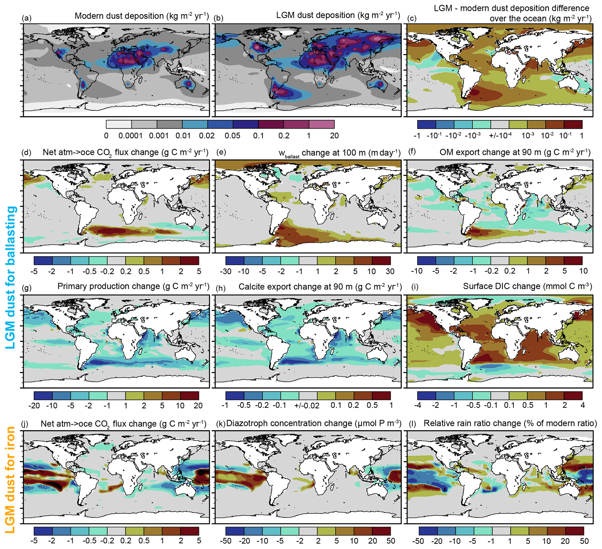
Figure 6 Effects of switching from modern to LGM dust deposition. (a) Modern dust deposition, (b) LGM dust deposition, and (c) LGM–modern dust deposition difference according to Mahowald et al. (2006). (d–i) LGM instead of modern dust deposition rates applied to particle ballasting (LGM_BALL) leading to changes of (d) the atmosphere–ocean CO₂ flux (positive into the ocean), (e) the common sinking speed w_ballast at 100 m depth, (f) the organic matter (OM) export at 90 m depth, (g) the vertically integrated primary production, (h) the calcite export at 90 m depth, and (i) the surface dissolved inorganic carbon (DIC) concentration. (j–l) LGM instead of modern dust deposition rates applied to the computation of dust-related iron input (LGM_IRON) leading to changes in (j) the atmosphere–ocean CO₂ flux, (k) the concentration of diazotrophs, and (l) the rain ratio (PIC∕POC ratio of the export flux at 90 m depth). The changes are computed from the first 100 years of the sensitivity simulations (LGM_BALL and LGM_IRON) relative to the control simulation with modern dust deposition (PI_BALLAST).

4.1 Role of LGM dust as ballast

The largest ballasting effect of the LGM dust in our sensitivity experiments occurs in the Southern Ocean off Patagonia. Here, the higher dust deposition rates lead to about 5 to 10 m d⁻¹ faster particle sinking at 100 m depth (Fig. 6e), which is equivalent to about a doubling of the sinking speed (compared to Fig. 2c). This faster sinking locally leads to a higher export production (Fig. 6f), to a reduced surface dissolved inorganic carbon concentration (Fig. 6i), and consequently to a positive downward net atmosphere–ocean CO₂ flux anomaly (Fig. 6d), which, accumulated over the first ∼3000 years, causes an atmospheric pCO₂ drawdown by about 4.5 ppmv (Fig. 5c). This anomalous ocean CO₂ uptake occurs despite a reduction in the globally integrated export production (Fig. 5d), as opposed to the locally enhanced export production off Patagonia (Fig. 6f). The smaller globally integrated export production is due to a reduced primary production over wide areas of the Atlantic, Pacific, and Indian Ocean, as well as parts of the Southern Ocean, just north of the area off Patagonia with enhanced organic matter export (Fig. 6g and f). This reduced primary production is consistent with a stronger nitrate depletion in surface waters (not shown) due to increased particle sinking speeds (Fig. 6e). Note that this nitrate depletion can have an effect on primary production globally, since nitrate is the least available nutrient for non-diazotroph phytoplankton everywhere in our model. However, at the same time, the production and export of calcite shells is reduced in the sensitivity simulation (Fig. 6h). Due to higher surface silicate concentrations (not shown), this calcite export reduction is disproportionately large (compared to the POC export reduction), which leads to a reduced rain ratio (Fig. 5f). This weakening of the calcium carbonate counter pump has a larger effect on the atmosphere–ocean CO₂ fluxes than the global reduction in the organic matter export, leading to a net ocean CO₂ uptake in the first ∼3000 years of our sensitivity experiment.

After about 3000 years, the ocean begins to release CO₂ into the atmosphere again, due to (1) the continuously decreasing export production (Fig. 5d; in response to nitrate depletion) and (2) the slowly recovering calcite production leading to an increasing particulate-inorganic-carbon-to-POC (PIC∕POC) export ratio anomaly (Fig. 5f).

The observed long-term CO₂ trends may also be affected by interactions with the sediment and by imbalances between sediment burial and weathering fluxes (see, e.g., Ridgwell, 2003). Since the weathering fluxes are the same in all sensitivity experiments (unchanged after the spin-up phase), a rough estimate of the role of sediment interactions can be derived from time series of the total organic carbon and calcite pools in the sediment (not shown). The organic carbon pool in the sediment in the experiment with LGM dust (LGM_BALL) grows faster than in the reference run with modern dust for ballasting (PI_BALLAST), which potentially contributes to the simulated ocean CO₂ uptake. This anomalous organic carbon pool trend amounts to an uptake of about 0.01 Gt C per year by the sediment, which is comparable in magnitude to the atmosphere–ocean CO₂ flux anomalies (Fig. 5b). Moreover, relative to PI_BALLAST, the sediment calcite pool in LGM_BALL is reduced by about 0.2×10¹⁶ mol Ca after the first 3000 years of the sensitivity experiment, which can be translated into a global mean ocean alkalinity increase of ∼3 mmol m⁻³, also potentially contributing to the simulated ∼10 mmol m⁻³ alkalinity increase in LGM_BALL at the surface.

4.2 Role of LGM dust as a source of iron

Iron fertilization, due to the iron contained in the dust (Sect. 2.2), also leads to a net CO₂ flux anomaly into the ocean. In our simulations, this anomalous CO₂ flux leads to an atmospheric pCO₂ drawdown by about 10 ppmv within 6500 years (Fig. 5c).

However, as evident from the lack of CO₂ flux anomalies in the Southern Ocean (Fig. 6j), this CO₂ drawdown in our sensitivity experiment is not due to the expected fertilization of phytoplankton growth by enhanced dust deposition in the Southern Ocean. Hence, the mechanism at work in our iron sensitivity experiment differs from the frequently studied classical iron hypothesis (Martin, 1990; Kumar et al., 1995; Watson et al., 2000; Werner et al., 2002; Bopp et al., 2003; Brovkin et al., 2007; Martinez-Garcia et al., 2014; Anderson et al., 2014; Ganopolski and Brovkin, 2017). The reason for this difference is, that, in contrast to observations (see Boyd et al., 2007, for a review), non-diazotroph phytoplankton growth in our reference simulations (for the standard set-up, PI_MARTIN, and the set-up with particle ballasting, PI_BALLAST) is limited by nitrate everywhere and nowhere by iron.

The simulated nitrogen-fixing cyanobacteria, on the other hand, have a higher iron demand than non-diazotroph phytoplankton (Falkowski et al., 1998; Berman-Frank et al., 2001; Kustka et al., 2003), which is also taken into account here by applying a Michaelis–Menten type iron limitation function with a high half-saturation constant (Paulsen et al., 2017). Moreover, since the diazotroph growth rate, unlike the non-diazotroph phytoplankton growth rate in our model, is not limited by the least available nutrient (Eq. 2 of Ilyina et al., 2013) but is proportional to the product of the limiting functions for temperature, iron, phosphate, and light (Eqs. 3 and 8 of Paulsen et al., 2017), the addition of iron can always lead to enhanced diazotroph growth. Consequently, we find enhanced diazotroph growth in particular in the tropical Pacific (Fig. 6k), which leads to a net positive downward atmosphere–ocean CO₂ flux anomaly locally (a reduced net CO₂ outgassing in the tropical Pacific; Fig. 6j). This CO₂ flux anomaly is caused by (1) enhanced organic matter export due to the enhanced diazotroph production (Fig. 5d) and (2) the associated reduction in the rain ratio in the tropical Pacific leading to a weakening of the calcium carbonate counter pump (Figs. 5f and 6l). A relative shift from calcifying to silicifying organisms, as reflected by enhanced opal export production (Fig. 5e), also contributes to the weakening of the calcium carbonate counter pump. However, the global mean sinking speed in LGM_IRON hardly differs from that in the reference run with modern dust (PI_BALLAST; Fig. 5a), suggesting that the ballasting effect of the additional opal is balanced by the effect of the reduced calcite export.

Even after 6500 years, the ocean still takes up additional CO₂ from the atmosphere. We attribute most of this long-term trend to a continuously enhanced organic matter export production (Fig. 5d) while the calcite export remains reduced, leading to a continuously lower PIC∕POC ratio (Fig. 5f) and to a reduced export of alkalinity. A slightly reduced calcite pool in the sediment in LGM_IRON compared to PI_BALLAST also potentially contributes a small portion to the simulated long-term atmospheric pCO₂ drawdown. The sediment calcite pool reduction is equivalent to an alkalinity increase in the water column of less than 2 mmol m⁻³, compared to a surface alkalinity increase of about 16 mmol m⁻³ after 6500 years in LGM_IRON. Less organic carbon is stored in the sediment in LGM_IRON compared to PI_BALLAST (not shown), which means that the exchange of organic matter between the sediment and the water column does not contribute to the simulated long-term ocean CO₂ uptake in LGM_IRON.

5 Summary and discussion

We estimate the potential effect of aeolian dust deposition changes on glacial–interglacial atmospheric pCO₂ variations by computing the sensitivity of the atmosphere–ocean CO₂ fluxes to LGM dust deposition (Sect. 4). To this end, we use the ocean circulation and carbon cycle model MPIOM/HAMOCC combined with a new particle ballasting parameterization (Sect. 2).

We find that the LGM dust deposition as estimated by Mahowald et al. (2006) leads to faster sinking and enhanced organic matter export off Patagonia and to a reduction in the calcium carbonate counter pump globally, which results in an anomalous (glacial) ocean CO₂ uptake that is equivalent to an atmospheric pCO₂ drawdown by 4.5 ppmv within 3000 years (Sect. 4.1).

The iron input associated with the LGM dust deposition causes a fertilization of diazotroph growth in the tropical Pacific, which leads to an additional atmospheric pCO₂ drawdown by about 10 ppmv within the 6500-year-long sensitivity experiment (Sect. 4.2), qualitatively supporting previous model results (Moore and Doney, 2007). The combination of these effects in response to the LGM dust deposition yields an atmospheric pCO₂ drawdown that is only slightly smaller than the sum of both effects (grey dashed line versus pink line in Fig. 5c), suggesting that synergistic effects play a minor role here. One negative synergistic effect, for example, which could explain the reduced CO₂ uptake in the combined experiment, is that the additional export production due to diazotroph iron fertilization may be reduced because nutrients are relocated due to particle ballasting.

According to previous modelling studies, iron fertilization in the Southern Ocean played a large role, leading to an atmospheric pCO₂ drawdown during the LGM by 15–40 ppmv (Watson et al., 2000; Bopp et al., 2003; Brovkin et al., 2007; Lambert et al., 2015; Ganopolski and Brovkin, 2017). However, in our simulations, due to the abundance of iron already for the applied modern dust deposition rates, non-diazotroph phytoplankton production is nowhere iron limited, and the additional iron input associated with the enhanced LGM dust deposition does not lead to a strengthening of the biological pump in the Southern Ocean. This lack of iron limitation could be addressed in future studies, for example by reducing the prescribed constant fraction of bioavailable iron within the dust in HAMOCC. It is also possible that this lack of iron limitation is due to an overestimation of the modern dust deposition rates by Mahowald et al. (2006). Both an older dust deposition estimate by Mahowald et al. (2005) as well as the (to our knowledge) most recent dust deposition estimate by Albani et al. (2016) find (locally in the Southern Ocean and South Atlantic as well as globally) smaller dust deposition rates than suggested by Mahowald et al. (2006). At the HAMOCC development group at the Max Planck Institute for Meteorology, since MPIOM revision 4283, which is included in the recent CMIP6-release of MPI-ESM (MPI-ESM version 1.2.01, MPIOM version 1.6.3, revision 4639), the dust deposition fields by Mahowald et al. (2006) were therefore replaced by the older dust deposition product by Mahowald et al. (2005) again, leading to iron limitation in the Southern Ocean in HAMOCC (Irene Stemmler, personal communication, 2018). However, in the model version used here, the dust by Mahowald et al. (2006) is used, and we do not switch back to the older dust deposition field, also because this older version does not provide an estimate of the dust deposition rates during the LGM. The recent estimate by Albani et al. (2016) does provide modern as well as LGM dust deposition estimates, but this product had not yet been published at the start of this project. The dust estimate by Albani et al. (2016) will be used in future versions of MPIOM/HAMOCC, but the implementation is still ongoing work. We expect that the addition of LGM dust anomalies using a version of MPIOM/HAMOCC that is newer than revision 4283 (using dust fields by Mahowald et al., 2005) or future versions (using dust fields by Albani et al., 2016) will lead to an additional atmospheric pCO₂ drawdown in response to the LGM dust deposition due to the fertilization of non-diazotroph phytoplankton in the Southern Ocean. This likely explains why the effect of the LGM iron addition on atmospheric pCO₂ is smaller in our simulation than suggested previously. Note that a more realistic iron fertilization response can also lead to modified synergies between iron fertilization and ballasting effects – any fertilization effect in the Southern Ocean would be enhanced or diminished by the associated ballast effect due to the resulting opal:POC, dust:POC, and PIC:POC ratio changes.

Mesocosm dust deposition experiments in the Mediterranean Sea (Wagener et al., 2010) and their numerical simulation (Ye et al., 2011) as well as more recent simulations of the global iron cycle (Ye and Völker, 2017) indicated that dust can also be a sink for dissolved bioavailable iron because the dust particles provide surfaces for the adsorption of dissolved bioavailable iron, leading to adsorptive scavenging. By not taking adsorptive scavenging by dust particles into account, we potentially overestimate the effect of dust deposition changes on iron fertilization.

Aggregate porosity and the degree of aggregate repackaging likely affects sinking speeds, too, as found for example in mesocosm experiments (Bach et al., 2016). In particular, opal ballast during diatom blooms did not lead to higher sinking speeds in the 25 m deep mesocosms, potentially due to the high porosities of the rather fresh aggregates. It is left for future studies to take into account the effect of porosity on the particle sinking speeds in HAMOCC. To avoid the computational expense of explicitly simulating aggregation and the porosities, the fraction of repackaged detritus (by zooplankton) to freshly produced detritus (e.g. by diatoms) could be computed and used to extend the parameterization of particle sinking speeds.

Also note that no aggregate sizes, size distributions or particle shapes are being computed in our ballasting parameterization, and hence potential effects of aggregate size distribution or shape changes on sinking velocities are neglected (see, e.g., Komar et al., 1981, for sinking speeds of approximately cylindrical fecal pellets).

Particle ballasting may play a larger role in glacial–interglacial pCO₂ variations than suggested by dust sensitivity alone. Variable ratios of opal∕POC or calcite∕POC can also affect particle sinking speeds via ballasting, and the ratios may have been modified by environmental change, such as variable temperature or variable input of weathering fluxes from land, sea level, or ocean circulation changes. For example, as discussed in Sect. 3.2, the efficiency of the soft tissue pump in OMZs is enhanced due to reduced remineralization rates, but corrosive conditions in OMZs tend to cause reduced calcite concentrations and thereby slower particle sinking speeds, reducing the higher remineralization length scale in OMZs; i.e. the role of oxygenation changes for the soft tissue pump and atmospheric pCO₂ in response to solubility, ocean circulation, or ecosystem variability (e.g. Jaccard and Galbraith, 2012) was potentially modified by particle ballasting. Transient simulations with the coupled MPI-ESM – including temperature and ocean circulation changes and their effects on OMZs – are envisaged to quantify the role of these potential additional particle ballasting feedbacks for glacial–interglacial CO₂ variability.