Scalable diagnostics for global atmospheric chemistry using Ristretto library (version 1.0)

We introduce a new set of algorithmic tools capable of producing scalable, low-rank decompositions of global spatiotemporal atmospheric chemistry data. By exploiting emerging randomized linear algebra algorithms, a suite of decompositions are proposed that extract the dominant features from big data sets (i.e., global atmospheric chemistry at longitude, latitude, and elevation) with improved interpretability. Importantly, our proposed algorithms scale with the intrinsic rank of the global chemistry space rather than the ever increasing spatiotemporal measurement space, thus allowing for the efficient representation and compression of the data. In addition to scalability, two additional innovations are proposed for improved interpretability: (i) a nonnegative decomposition of the data for improved interpretability by constraining the chemical space to have only positive expression values (unlike PCA analysis); and (ii) sparse matrix decompositions, which threshold small weights to zero, thus highlighting the dominant, localized spatial activity (again unlike PCA analysis). Our methods are demonstrated on a full year of global chemistry dynamics data, showing the significant improvement in computational speed and interpretability. We show that the decomposition methods presented here successfully extract known major features of atmospheric chemistry, such as summertime surface pollution and biomass burning activities.

1 Introduction

Dimensionality reduction is a critically enabling aspect of machine learning and data science in the era of big data. Specifically, extracting the dominant low-rank features from a high-dimensional data matrix X allows one to efficiently perform tasks associated with clustering, classification, reconstruction, and prediction (forecasting). Commonly used linear dimensionality reduction methods are typically based upon singular value decomposition (SVD) which allows one to exploit covariances manifest in the data (Cunningham and Ghahramani, 2015). Thus, the analysis of big data, such as the atmospheric chemistry data considered here, relies on a variety of matrix decomposition methods which seek to exploit low-rank features exhibited by the high-dimensional data. Despite our ever-increasing computational power, the emergence of large-scale data sets has severely challenged our ability to analyze data using traditional matrix algorithms, especially for ever increasing refinements of computational models.

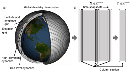
Figure 1 Atmospheric chemistry simulation on a global mesh with discretized longitude, latitude, and elevation (panel a modified from NOAA). Each illustrated grid cell contains time-series data for the atmospheric chemistry dynamics. Well resolved simulations generate massive data sets that are often not amenable to diagnostic analysis. Our proposed algorithms offer a scalable architecture for the analysis of global spatiotemporal data. As shown in the two right panels (b), the original data matrix $\mathbf{X}\in {\mathbb{R}}^{m\times n}$, where m is the number of grid points and n is the number of snapshots, can be downsampled (here via random column sampling) to form the matrix $\mathbf{Y}\in {\mathbb{R}}^{m\times k}$, where k≪n. Although random column selection is shown, we can also use a random measurement matrix to sample the data as shown in Sect. 3.

In this work, we are specifically concerned with time-series measurements of the concentration of chemical species collected from spatial locations in the atmosphere, illustrated in Fig. 1. On a global scale (longitude, latitude, and elevation), this data can be exceptionally high-dimensional so as to be not computationally tractable. Thus, computationally scalable methods are required for the analysis of atmospheric chemistry dynamics. Indeed, atmospheric chemistry is an exceptionally high-dimensional problem as it involves hundreds of chemical species that are coupled with each other via a set of ordinary differential equations. Models of atmospheric chemistry that are used to simulate the spatiotemporal evolution of these chemical constituents need to keep track of each chemical species on a global scale (longitude, latitude, and elevation) and at each point in time. The resulting data sets – used for scientific analysis or required for subsequent restarts of the model – quickly become massive, especially as the horizontal model resolution steadily increases. For example, a single snapshot of the chemical state of an atmospheric chemistry model at 25 km×25 km horizontal resolution requires 60 GB of storage space.

To tackle this challenge, we present a variety of emerging matrix decomposition methods that can be used for scalable diagnostics of global atmospheric chemistry dynamics. Specifically, we use randomized linear algebra methods (Halko et al., 2011; Mahoney, 2011; Drineas and Mahoney, 2016; Erichson et al., 2016, 2017a) to extract the dominant, low-rank mode structures from a full three-dimensional atmospheric chemistry data set. These methods are highly scalable and can thus be used on emerging big data sets describing global chemistry dynamics, providing a useful tool for scientific discovery and analysis. Furthermore, they offer an alternative approach for the storage of large-scale atmospheric chemistry data. Importantly, randomized methods are an efficient alternative to distributed computing if these computational resources are not available. For instance, Gittens et al. (2018) can compute the SVD of a 2.2 TB (terabyte) data set in about 60 s, given a supercomputer with many nodes. However, if supercomputing is not available, randomized methods offer an attractive alternative which does not require expensive computation hours on a cluster.

The paper is outlined as follows: Sect. 2 gives an overview of the global chemistry simulation engine used to produce the data of interest. Section 3 highlights the various decomposition methods that can be produced using randomized linear algebra techniques. Section 4 shows the results of the dimensionality reduction procedures, highlighting the effectiveness of each technique. Section 5 shows how such techniques can be used for data compression and reduced order models, enabling compact representations of the data for a variety of broader scientific studies. Section 6 provides concluding remarks and a brief outlook for data sciences applied to atmospheric dynamics and global chemistry analysis.

2 Atmospheric chemistry model and data

Understanding the composition of the atmosphere is critical for a wide range of applications, including air quality, chemistry–climate interactions, and global biogeochemical cycling. Chemical transport models (CTMs) are used to simulate the evolution of atmospheric constituents in space and time (Brasseur and Jacob, 2017). A CTM solves the system of coupled continuity equations for an ensemble of m species with number density vector $\mathit{n}={\left(n_{\mathrm{1}},\mathrm{\dots },n_m\right)}^{\mathrm{T}}$ via operator splitting of transport and local processes:

$$\begin{array}{}\text{(1)}& {\displaystyle \frac{\partial n_i}{\partial t}}=-\mathrm{\nabla }\cdot \left(n_i\mathit{U}\right)+\left(P_i-L_i\right)\left(\mathit{n}\right)+E_i-D_{i}i\in \left[\mathrm{1},m\right],\end{array}$$

where U is the wind vector, (P_i−L_i)(n) is the (local) chemical production and loss terms, E_i is the emission rate, and D_i is the deposition rate of species i. The transport operator

$$\begin{array}{}\text{(2)}& {\displaystyle \frac{\partial n_i}{\partial t}}=-\mathrm{\nabla }\cdot \left(n_i\mathit{U}\right)i\in \left[\mathrm{1},m\right]\end{array}$$

involves spatial coupling across the model domain but no coupling between chemical species, whereas the chemical operator

$$\begin{array}{}\text{(3)}& {\displaystyle \frac{\mathrm{d}{n}_i}{\mathrm{d}t}}=\left(P_i-L_i\right)\left(\mathit{n}\right)+E_i-D_{i}i\in \left[\mathrm{1},m\right]\end{array}$$

includes no spatial coupling but the species are chemically linked through a system of ordinary differential equations (ODEs).

Chemistry models repeatedly solve Eqs. (2) and (3), which require full knowledge of the chemical state of the atmosphere at all locations and times. The resulting four-dimensional data sets (longitude, latitude, levels, and species) can become massive, which makes it unpractical to output them at a high temporal frequency. As a consequence, model output is generally restricted to a few selected species of interest (e.g., ozone), whereas the full model state is only output very infrequently, e.g., to archive the information for future model restarts (“restart file”). Here we show that the chemical state of a CTM, such as GEOS-Chem, has distinct low-ranked features and exploiting these properties using modern diagnostic tools such as variable reduction or subsampling makes it possible to represent the same amount of information in a computationally more efficient manner. While we focus on identifying low-ranked features across the spatiotemporal dimension (i.e., for each species separately), the methods presented could similarly (and independently) be applied across the species domain.

2.1 Global atmospheric chemistry simulations

The reference simulation of atmospheric chemistry was generated using the GEOS-Chem model. GEOS-Chem (http://geos-chem.org, last access: 11 April 2019) is an open-source global model of atmospheric chemistry that is used by over a hundred active research groups in 25 countries around the world for a wide range of applications. The code is freely available through an open license (http://acmg.seas.harvard.edu/geos/geos_licensing.html, last access: 11 April 2019). GEOS-Chem can be run in off-line mode as a chemical transport model (CTM) (Bey et al., 2001; Eastham et al., 2018) or as an online component within the NASA Goddard Earth system model (GEOS) (Long et al., 2015; Hu et al., 2018). In this study we use the off-line version of GEOS-Chem v11-01, driven by archives of assimilated meteorological data from the GEOS Forward Processing (GEOS-FP) data stream of the NASA Global Modeling and Assimilation Office (GMAO). The model chemistry scheme includes detailed HO_x–NO_x–VOC–ozone–BrO_x tropospheric chemistry as originally described by Bey et al. (2001), with addition of BrO_x chemistry from Parrella et al. (2012), and updates to isoprene oxidation as described by Mao et al. (2013). Dynamic and chemical time steps are 30 and 20 min, respectively. Stratospheric chemistry is modeled using a linearized mechanism as described by Murray et al. (2012).

We performed a 1-year simulation of GEOS-Chem (July 2013–June 2014) at $\mathrm{4}{}^{\circ }\times \mathrm{5}{}^{\circ }$ horizontal resolution to generate a comprehensive set of atmospheric chemistry model diagnostics. For every chemistry time step, the concentrations of all 143 chemical constituents were archived immediately before and after chemistry (in units of molecules cm⁻³). The difference between these concentration pairs is the species tendencies due to chemistry (expressed in units of molecules cm⁻³ s⁻¹). As the solution of chemical kinetics is also a function of the environment, we further output key environmental variables such as temperature, pressure, water vapor, and photolysis rates. The latter are computed online by GEOS-Chem using the Fast-JX code of Bian and Prather (2002) as implemented in GEOS-Chem by Mao et al. (2010) and Eastham et al. (2014). Thus, at every time step, the data set consists of nfeatures $=\mathrm{143}+\mathrm{91}+\mathrm{3}+\mathrm{143}=\mathrm{380}$ data points at every grid location. We restrict our analysis to the lowest 30 model levels to avoid influence from the stratosphere. The resulting data set has the following dimensions: $n\text{long}\times n\text{lat}\times n\text{lev}\times n\text{times}\times n\text{features}=\mathrm{72}\times \mathrm{46}\times \mathrm{30}\times \mathrm{26}\mathrm{280}\times \mathrm{380}=\mathrm{9.9}\times {\mathrm{10}}^{\mathrm{11}}$.

2.2 Data preprocessing

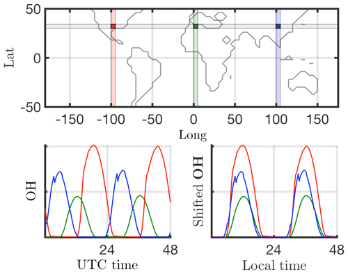
Many dimensionality reduction techniques rely on an underlying singular value decomposition of the data that extracts correlated patterns in the data. A fundamental weakness of such SVD-based approaches is the inability to efficiently handle invariance in the data. Specifically, translational and/or rotational invariance of low-rank features in the data are not well captured (Kutz, 2013; Kutz et al., 2016). One of the key environmental variables driving the chemistry is photolysis rate; therefore, the absolute concentrations of many chemicals of interest accordingly “turn on” and are nonzero during daytime, and “turn off” or go to zero during the night. The time series of absolute chemical concentrations exhibit a translating wave traversing the globe from east to west with constant velocity. The time series for the chemical species OH (hydroxyl radical) is plotted with respect to UTC time for one latitude/elevation and three different longitudes on bottom left in Fig. 2, highlighting the translational invariance in the absolute concentration data. Any SVD-based approach will be unable to capture this translational invariance and correlate across snapshots in time, producing an artificially high dimensionality, i.e., a higher number of modes would be needed to characterize the dynamics due to translation (Kutz, 2013). To overcome this issue the time series for each grid point are shifted to align with the local GMT time, as shown on bottom right in Fig. 2. With the local times for each grid point aligned, SVD-based dimensionality reduction techniques can now identify and isolate coherent low-dimensional features in the data.

Figure 2 Shifting the data for each cell in time to align the local time zones across a latitude to the prime meridian (Long =0) LT, shown here for the OH absolute concentration for Lat =30.

3 Scalable matrix decompositions for diagnostics

The following subsections detail a probabilistic framework for matrix decompositions that includes a nonnegative matrix factorization as well as a sparsity-promoting technique. The mathematical architectures proposed provide scalable computational tools for the analysis of global chemistry dynamics. Moreover, by providing three different dimensionality architectures, a more nuanced objective analysis of the dominant spatiotemporal patterns that emerge in the global chemistry dynamics is achieved. The standard analysis would be a simple randomized SVD decomposition, whereby the dominant correlated structures are computed. A more refined approach to computing the dominant correlated structures involves restricting the dominant spatiotemporal structures to reasonable physical considerations. Specifically, the nonnegative matrix factorization restricts all chemicals to positive concentrations, a restriction which is physically motivated and especially important for diagnostics when physical interpretation is required. The randomized SVD will generally produce a negative concentration of chemicals in individual modes, but the overall concentration is positive when the modes are summed together. Likewise, the sparse PCA analysis zeroes out very small concentrations so that the modes extracted highlight only nonzero contributions to the dynamics. This is an important modification of the randomized SVD, as it generally produces all nonzero entries in the modal structures, regardless if it is physical. This is due to the least-square nature of the SVD algorithm. Again, a sparsification penalty produces modes where only the dominant coefficients are nonzero. What one chooses to use may depend strongly on the intended application. Regardless, the suite of methods allows for a more nuanced view of the data.

3.1 Probabilistic framework for low-rank approximations

Assume that the data matrix $\mathbf{X}\in {\mathbb{R}}^{m\times n}$ has rank r, where $r\le min\left\{m,n\right\}$. The objective of a low-rank matrix approximation to the input data matrix X is to find two smaller matrices

$$\begin{array}{}\text{(4)}& {\displaystyle }\begin{array}{cccc}\mathbf{X}& \approx & \mathbf{E}& \mathbf{F}\\ m\times n& & m\times r& r\times n\end{array},\end{array}$$

where the columns of E span the column space of X, and the rows of F span the row space of X. These factors can be stored much more efficiently, and can be used to approximate the massive input data matrix and summarize the interesting low-dimensional features which are often interpretable. Probabilistic algorithms have been established over the past 2 decades to compute such computationally tractable smaller matrix approximations. We seek a near-optimal low-dimensional approximation of the input data matrix X using a probabilistic framework as formulated by Halko et al. (2011). Conceptually, the probabilistic framework splits the task of computing a near-optimal low-rank approximation into two logical stages:

• Stage A. Compute a low-dimensional subspace that approximates the column space of X. We aim to find a near-optimal basis $\mathbf{Q}\in {\mathbb{R}}^{m\times k}$ with orthonormal columns such that

  $$\begin{array}{}\text{(5)}& {\displaystyle }\mathbf{X}\approx {\mathbf{QQ}}^{\mathrm{T}}\mathbf{X}\end{array}$$

  is satisfied, where k is the desired target rank. Random projections are used to sample the column space of the input matrix X. Random projections are data agnostic, and are constructed by first drawing a set of k independent random vectors ${\left\{{\mathit{\omega }}_i\right\}}_{i=\mathrm{1}}^k$, for instance, from the standard normal distribution; X is then mapped to the low-dimensional space to obtain the random sample projections y_i :=Xω_i for $i=\mathrm{1},\mathrm{\dots },k$. Define a random test matrix $\mathbf{\Omega }=\left[{\mathit{\omega }}_{\mathrm{1}},\mathrm{\dots },{\mathit{\omega }}_k\right]\in {\mathbb{R}}^{n\times k}$, where the sample random projections form the sampling matrix $\mathbf{Y}\in {\mathbb{R}}^{m\times k}$ are given by

  $$\begin{array}{}\text{(6)}& {\displaystyle }\mathbf{Y}:=\mathbf{X}\mathbf{\Omega }\end{array}$$

  Y is denoted as the sketch matrix. The columns of Yare now orthonormalized using the QR-decomposition Y=QR, where Q is the near-optimal low-dimensional basis that approximates the column space of the input data matrix. For most real-world data matrices with a gradually decaying singular value spectrum, this basis matrix Q does not provide a good approximation for the column space of the input data matrix. A much better approximation is obtained by the following:

  • Oversampling. For target rank k, for most data matrices we may have nonzero singular values ${\left\{{\mathit{\sigma }}_i\right\}}_{i=k+\mathrm{1}}^{min\left(m,n\right)}$. As a consequence, the sketch Y obtained above does not exactly span the column space of the input data matrix. Oversampling, i.e., using $l=k+p$ random projections to form the sketch overcomes this issue, and a small number of additional projections $p=\left\{\mathrm{5},\mathrm{10}\right\}$ is often sufficient to obtain a good basis comparable to the best possible basis (Martinsson, 2016).

  • Power iteration scheme. The quality of Q can be improved by the concept of power sampling iterations (Halko et al., 2011; Rokhlin et al., 2010). An improved sketch is defined under this concept as Y := X^(q)Ω, where q is an integer specifying the number of power iterations. This process enforces a more rapid decrease of the singular values, enabling the algorithm to sample the relevant information related to the dominant singular values while the unwanted information is suppressed. As few as $q=\left\{\mathrm{1},\mathrm{2},\mathrm{3}\right\}$ power iterations can considerably improve the accuracy of the approximation. Orthogonalizing the sketch between each iteration further improves the numerical stability of the algorithm.

• Stage B. At this stage, we form a smaller matrix B

  $$\begin{array}{}\text{(7)}& {\displaystyle }\mathbf{B}:={\mathbf{Q}}^{\mathrm{T}}\mathbf{X}\in {\mathbb{R}}^{l\times n}\end{array}$$

  In other words, we restrict the high-dimensional input matrix to the low-dimensional space spanned by the near-optimal basis Q obtained in Stage A. Geometrically, this is a projection which takes points in a high-dimensional measurement space to a low-dimensional space while maintaining the structure in a Euclidean sense.

The probabilistic framework detailed above is referred to as the QB decomposition of the input data matrix X, and yields the following low-rank approximation:

$$\begin{array}{}\text{(8)}& {\displaystyle }\begin{array}{cccc}\mathbf{X}& \approx & \mathbf{Q}& \mathbf{B}\\ m\times n& & m\times l& l\times n\end{array}\end{array}$$

Note that the randomized algorithm outlined here requires two passes over the entire data matrix to construct the basis matrix Q. The near-optimal low-rank approximation $\mathbf{B}\in {\mathbb{R}}^{l\times n}$, where $l\ll min\left(m,n\right)$, can now be used instead of the data matrix X to compute traditional deterministic matrix decompositions for data analysis. The QB decomposition can also be extended to distributed and parallel computing, see Voronin and Martinsson (2015).

3.2 Randomized singular value decomposition

The data matrix $\mathbf{X}\in {\mathbb{R}}^{m\times n}$ has a singular value decomposition (SVD) of the form

$$\begin{array}{}\text{(9)}& {\displaystyle }\mathbf{X}=\mathbf{U}\mathbf{\Sigma }{\mathbf{V}}^{\mathrm{T}}\end{array}$$

with unitary matrices $\mathbf{U}=\left[{\mathbf{u}}_{\mathrm{1}},\mathrm{\dots },{\mathbf{u}}_m\right]\in {\mathbb{R}}^{m\times m}$ and $\mathbf{V}=\left[{\mathbf{v}}_{\mathrm{1}},\mathrm{\dots },{\mathbf{v}}_n\right]\in {\mathbb{R}}^{n\times n}$ orthonormal such that U^TU=I and V^TV=I. The left singular vectors in U provide a basis for the range (column space), and the right singular vectors in V provide a basis for the domain (row space) of the data matrix X. The rectangular diagonal matrix $\mathbf{\Sigma }\in {\mathbb{R}}^{m\times n}$ has the corresponding nonnegative singular values ${\mathit{\sigma }}_{\mathrm{1}}\ge \mathrm{\dots }\ge {\mathit{\sigma }}_n\ge \mathrm{0}$, which describe the spectrum of the data. Low-rank matrices have rank r that is much smaller than the dimension of the measurement space, i.e., $r\ll m,n$ and the singular values $\left\{{\mathit{\sigma }}_i:\ge r+\mathrm{1}\right\}$ are zero. The corresponding singular vectors span the left and right null spaces of the matrix. In practical applications the data matrix are often contaminated by errors making its effective rank smaller than the exact rank r. In such cases the matrix can be well approximated by only those singular vectors which correspond to the singular values of a significant magnitude, and a reduced version of the SVD is computed:

$$\begin{array}{ll}{\displaystyle }{\mathbf{X}}_k& {\displaystyle }:={\mathbf{U}}_k{\mathbf{\Sigma }}_k{\mathbf{V}}_k\\ \text{(10)}& {\displaystyle }& {\displaystyle }=\left[{\mathbf{u}}_{\mathrm{1}},\mathrm{\dots },{\mathbf{u}}_k\right]\text{diag}\left({\mathit{\sigma }}_{\mathrm{1}},\mathrm{\dots },{\mathit{\sigma }}_k\right){\left[{\mathbf{v}}_{\mathrm{1}},\mathrm{\dots },{\mathbf{v}}_k\right]}^{\mathrm{T}},\end{array}$$

where k denotes the desired target rank of the approximation. Choosing an optimal k is highly dependent on the task. If a highly accurate reconstruction of the original data is desired, then k should be chosen closer to the effective rank of the data matrix. Conversely, if a very low-dimensional representation of dominant features is desired, then k might be chosen to be much smaller. The Eckart–Young theorem (Eckart and Young, 1936) states that the low-rank SVD provides the optimal rank-k reconstruction of a matrix in the least-squares sense

$$\begin{array}{}\text{(11)}& {\displaystyle }{\mathbf{X}}_k:=\underset{\text{rank}\left(\mathbf{X}{{}^{\prime }}_k\right)}{\text{argmin}}∥\mathbf{X}-\mathbf{X}{{}^{\prime }}_k∥\end{array}$$

with the reconstruction error in the spectral and Frobenius norm given by

$$\begin{array}{}\text{(12)}& {\displaystyle }{∥\mathbf{X}-{\mathbf{X}}_k∥}_{\mathrm{2}}={\mathit{\sigma }}_{k+\mathrm{1}}\left(\mathbf{X}\right)\end{array}$$

and

$$\begin{array}{}\text{(13)}& {\displaystyle }{∥\mathbf{X}-{\mathbf{X}}_k∥}_{\mathrm{F}}=\sqrt{\sum _{j=k+\mathrm{1}}^{min\left(m,n\right)}{\mathit{\sigma }}_j^{\mathrm{2}}\left(\mathbf{X}\right)}\end{array}$$

For massive data sets, however, the cost of computing the full SVD of the data matrix X is order O(mn²), from which the first k components can then be extracted to form X_k. Randomized algorithms are computationally efficient and `surprisingly' reliable; these techniques can be used to obtain an approximate rank-k SVD at a substantially more efficient cost of O(mnk).

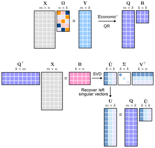
The probabilistic framework is used to obtain a near-optimal low-rank approximation $\mathbf{B}\in {\mathbb{R}}^{l\times n}$, where $l\ll min\left(m,n\right)$. This can now be used instead of the data matrix X, and a full SVD of B is computed

$$\begin{array}{}\text{(14)}& {\displaystyle }\mathbf{B}=\stackrel{\mathrm{̃}}{\mathit{U}}\mathbf{\Sigma }{\mathit{V}}^{\mathrm{T}}\end{array}$$

to give the first l right singular vectors $\mathit{V}\in {\mathbb{R}}^{n\times l}$ and the corresponding singular values $\mathbf{\Sigma }\in {\mathbb{R}}^{l\times l}$. The left singular vectors $\mathit{U}\in {\mathbb{R}}^{m\times l}$ are recovered from the approximate left singular vectors $\stackrel{\mathrm{̃}}{\mathit{U}}\in {\mathbb{R}}^{l\times l}$ using the near-optimal basis matrix Q

$$\begin{array}{}\text{(15)}& {\displaystyle }\mathit{U}\approx \mathbf{Q}\stackrel{\mathrm{̃}}{\mathit{U}}\end{array}$$

For the absolute concentration data matrix, note that the right singular vectors V are temporal and the left singular vectors U are the spatial dominant features of the system. We also compute a cumulative energy spectrum from the singular values, the energy in the first j dominant modes is given by

$$\begin{array}{}\text{(16)}& {\displaystyle \frac{{\sum }_{i=\mathrm{1}}^j{\mathit{\sigma }}_i^{\mathrm{2}}}{\text{Total energy in the data}}},\end{array}$$

where the total energy in the data is computed using the Frobenius norm as ${∥\mathbf{X}∥}_{\mathrm{F}}^{\mathrm{2}}$.

The algorithm architecture is conceptually outlined in Fig. 3. This shows the basic architecture and the structure which allows for a rapid approximation of the left and right singular values and eigenvectors.

Figure 3 Illustration of the randomized matrix decomposition technique. The random sampling matrix Ω is used to produce a new matrix Y which can be decomposed using a QR decomposition. This leads to the construction of the matrix B which is used for approximating the left and right singular vectors.

3.3 Randomized nonnegative matrix factorization

A significant drawback of commonly used dimensionality reduction techniques, such as SVD based principal component analysis (PCA), is that they permit both positive and negative terms in their components. In many data applications, such as in the absolute concentration, negative terms fail to be interpretable in a physically meaningful sense, i.e., chemical concentrations are not negative. To address this problem the set of basis vectors are constrained to nonnegative terms (Lee and Seung, 1999; Paatero and Tapper, 1994) – this paradigm is the nonnegative matrix factorization (NMF). NMF has emerged as a powerful dimension reduction tool that allows the computation of a sparse, parts-based representation of physically meaningful additive factors that describe coherent structures within the data. Given the data matrix $\mathbf{X}\in {\mathbb{R}}^{m\times n}$, the NMF has to find two matrices of a much lower rank

$$\begin{array}{}\text{(17)}& {\displaystyle }\begin{array}{cccc}\mathbf{X}& \approx & \mathbf{W}& \mathbf{H}\\ m\times n& & m\times k& k\times n\end{array},\end{array}$$

where k is the target rank. The SVD finds an exact solution of this problem in the least-squares sense, as detailed in the previous section, but the resulting factors are not guaranteed to be physically meaningful, i.e., positive values. NMF, in comparison, gives an additive parts-based representation of the data that preserves useful properties such as sparsity and nonnegativity by imposing additional nonnegativity constraints: W≥0 and H≥0. The sparse parts-based features have an intuitive interpretation which has been exploited in environmental modeling (Paatero and Tapper, 1994). In environmental data, the error estimates of data can be widely varying and nonnegativity is often an essential feature of the underlying models (Juntto and Paatero, 1994; Lee et al., 1999; Paterson et al., 1999; Xie et al., 1999). Traditionally, the NMF problem is formulated as the following optimization problem:

$$\begin{array}{}\text{(18)}& {\displaystyle }\begin{array}{cccc}\mathrm{minimize}& f\left(\mathbf{W},\mathbf{H}\right)& =& {∥\mathbf{X}-\mathbf{WH}∥}_{\mathrm{F}}^{\mathrm{2}}\\ \mathrm{subject}\mathrm{to}& \mathbf{W}\ge \mathrm{0}& \text{and}& \mathbf{H}\ge \mathrm{0}\end{array}\end{array}$$

This optimization problem is nonconvex and ill-posed. As no convexification exists to simplify the optimization, no exact or unique solution is guaranteed (Gillis, 2017). Therefore, different NMF algorithms can produce distinct decompositions that minimize the objective function. As the problem is nonconvex with respect to both factors W and H, most NMF algorithms divide the problem into simpler subproblems that have closed form solutions. The convex subproblem is solved by keeping one factor fixed while updating the other, and alternating and iterating until convergence. The hierarchical alternating least squares (HALS) is one variant of this method, proved to be highly efficient (Cichocki and Phan, 2009), and this is the algorithm employed here for computing the NMF.

Block coordinate descent (BCD) iterative methods fix a block of components and optimize with respect to the remaining components. The factors W and H are initialized and updated by fixing most terms except for the block comprised of the jth column ${\mathbf{W}}_{\left(:,j\right)}$ and the jth row ${\mathbf{H}}_{\left(j,:\right)}$. HALS approximately minimizes the cost function in Eq. (18) with respect to the remaining k−1 components

$$\begin{array}{}\text{(19)}& {\displaystyle }\mathrm{\text{minimize}}{J}_j\left({\mathbf{W}}_{\left(:,j\right)},{\mathbf{H}}_{\left(j,:\right)}\right)={∥{\mathbf{R}}^{\left(j\right)}-{\mathbf{W}}_{\left(:,j\right)}{\mathbf{H}}_{\left(j,:\right)}∥}_{\mathrm{F}}^{\mathrm{2}},\end{array}$$

where R^(j) is the jth residual

$$\begin{array}{}\text{(20)}& {\displaystyle }{\mathbf{R}}^{\left(j\right)}:=\mathbf{X}-\sum _{i\ne j}^k{\mathbf{W}}_{\left(:,i\right)}{\mathbf{H}}_{\left(i,:\right)}\end{array}$$

Gradients are derived to find the stationary points for both components, for details see Cichocki and Phan (2009).

For massive data sets randomness is again employed to replace the high-dimensional input data matrix $\mathbf{X}\in {\mathbb{R}}^{m\times n}$ by its near-optimal low-rank approximation $\mathbf{B}\in {\mathbb{R}}^{l\times n}$, where $l\ll min\left(m,n\right)$, with the exception that the entries of Ω are drawn independently from the uniform distribution with support $\mathit{\omega }\in \left[\mathrm{0},\mathrm{1}\right]$. We now have the following optimization problem:

$$\begin{array}{}\text{(21)}& {\displaystyle }\begin{array}{cccc}\mathrm{minimize}& \stackrel{\mathrm{̃}}{f}\left(\stackrel{\mathrm{̃}}{\mathbf{W}},\mathbf{H}\right)& =& {∥\mathbf{B}-\stackrel{\mathrm{̃}}{\mathbf{W}}\mathbf{H}∥}_{\mathrm{F}}^{\mathrm{2}}\\ \mathrm{subject}\mathrm{to}& \mathbf{Q}\stackrel{\mathrm{̃}}{\mathbf{W}}\ge \mathrm{0}& \text{and}& \mathbf{H}\ge \mathrm{0},\end{array}\end{array}$$

where the nonnegativity constraints need apply to the high-dimensional factor matrix W, but not necessarily to $\stackrel{\mathrm{̃}}{\mathbf{W}}$, as $\stackrel{\mathrm{̃}}{\mathbf{W}}$ can be rotated back to high-dimensional space using the approximate relation $\mathbf{W}\approx \mathbf{Q}\stackrel{\mathrm{̃}}{\mathbf{W}}$. As QQ^T≠I, Eq. (21) can only be solved approximately. The randomized HALS algorithm is formulated as

$$\begin{array}{}\text{(22)}& {\displaystyle }\mathrm{minimize}{J}_j\left({\stackrel{\mathrm{̃}}{\mathbf{W}}}_{\left(:,j\right)},{\mathbf{H}}_{\left(j,:\right)}\right)={∥{\stackrel{\mathrm{̃}}{\mathbf{R}}}^{\left(j\right)}-{\stackrel{\mathrm{̃}}{\mathbf{W}}}_{\left(:,j\right)}{\mathbf{H}}_{\left(j,:\right)}∥}_{\mathrm{F}}^{\mathrm{2}},\end{array}$$

where R^(j) is the jth compressed residual

$$\begin{array}{}\text{(23)}& {\displaystyle }{\stackrel{\mathrm{̃}}{\mathbf{R}}}^{\left(j\right)}:=\mathbf{B}-\sum _{i\ne j}^k{\stackrel{\mathrm{̃}}{\mathbf{W}}}_{\left(:,i\right)}{\mathbf{H}}_{\left(i,:\right)}\end{array}$$

The components are updated again by deriving the gradients. For further details, such as initialization techniques, stopping criterion, and variants of randomized HALS we refer to Erichson et al. (2018a).

For the absolute chemistry concentration data matrix, the columns of the factor W are the spatial modes while those of factor H are the temporal modes. The randomized NMF algorithm starts with an initial guess derived from a SVD of the data matrix, and returns the W, H factors with columns that are not ordered. The 2-norm of the columns is computed, and the columns are normalized and ordered. A product of the ordered column-wise 2-norms gives the ”spectrum” for the decomposition. From this spectrum a cumulative energy spectrum is computed similar to Eq. (16).

3.4 Sparse randomized principal component analysis

Principal component analysis is a prevalent technique for dimensionality reduction, it exploits relationships among points in high-dimensional space to construct a new set of uncorrelated low-dimensional variables or principal components (PCs). The first PC explains most of the variation in the data, the second PC accounts for the second greatest variance in the data, and so on. For the data matrix $\mathbf{X}\in {\mathbb{R}}^{m\times n}$, which has now been centered with zero mean, with m being the number of observations and n being the number of variables, the PCs z_i∈ℝ^m are constructed as a weighted linear combination of the original variables

$$\begin{array}{}\text{(24)}& {\displaystyle }{\mathbf{z}}_i=\mathbf{X}{\mathit{w}}_i,\end{array}$$

where w_i∈ℝⁿ is a vector of the corresponding weights, also denoted as modes or basis functions. Expressed concisely,

$$\begin{array}{}\text{(25)}& {\displaystyle }\mathbf{Z}=\mathbf{XW}\end{array}$$

with $\mathbf{Z}=\left[{\mathbf{z}}_{\mathrm{1}},\mathrm{\dots },{\mathbf{z}}_n\right]\in {\mathbb{R}}^{m\times n}$ and $\mathbf{W}=\left[{\mathit{w}}_{\mathrm{1}},\mathrm{\dots },{\mathit{w}}_n\right]\in {\mathbb{R}}^{n\times n}$. In most dimensionality reduction applications only the first k PCs will be of interest to visualize the data in a low-dimensional space, and as the relevant features used for data clustering, classification and regression. The problem of finding the PCs can be formulated as a variance maximization problem or as a least-squares problem, i.e., minimizing the sum of squared residual errors with orthogonality constraints on the weight matrix as

$$\begin{array}{}\text{(26)}& {\displaystyle }\begin{array}{ccc}\underset{\mathbf{W}}{\text{minimize}}f\left(\mathbf{W}\right)& =& \frac{\mathrm{1}}{\mathrm{2}}{∥\mathbf{X}-{\mathbf{XWW}}^{\mathrm{T}}∥}_{\mathrm{F}}^{\mathrm{2}}\\ \mathrm{subject}\mathrm{to}{\mathbf{W}}^{\mathsf{T}}\mathbf{W}& =& \mathbf{I}\end{array}\end{array}$$

The classic PCA approach outlined above generates global PCs as a linear combination of all n variables; hence, this approach tends to mix or blend various spatiotemporal scales and fails to identify and isolate underlying governing dynamics acting at each scale. Sparse principal component analysis (SPCA) is a variant which provides interpretable PCs with localized spatial support, providing a “parsimonious” decomposition through sparsity promoting regularizers on the weights W. Each of the sparse weight vectors w_i have only a few nonzero values; therefore, we get a linear combination of only a few of the original variables. The SPCA is mathematically formulated as a variant of PCA outlined in Eq. (26) as

$$\begin{array}{}\text{(27)}& {\displaystyle }\begin{array}{ccc}\underset{\mathbf{A},\mathbf{W}}{\text{minimize}}f\left(\mathbf{A},\mathbf{W}\right)& =& \frac{\mathrm{1}}{\mathrm{2}}{∥\mathbf{X}-{\mathbf{XWA}}^{\mathrm{T}}∥}_{\mathrm{F}}^{\mathrm{2}}+\mathit{\psi }\left(\mathbf{W}\right)\\ \mathrm{subject}\mathrm{to}{\mathbf{A}}^{\mathrm{T}}\mathbf{A}& =& \mathbf{I},\end{array}\end{array}$$

where W is now a sparse weight matrix, and A is an orthonormal inverse transform matrix, i.e., the data can be approximately constructed as $\stackrel{\mathrm{̃}}{\mathbf{X}}={\mathbf{ZA}}^{\mathrm{T}}$, where Z is the PC matrix given by Eq. (25). In Eq. (27), ψ is a sparsity inducing regularizer such as

• ℓ₀ norm defined as the number of nonzero elements in a vector x, which is constrained to be ≪n

  $$\begin{array}{}\text{(28)}& {\displaystyle }{\mathit{\psi }}_{\mathrm{0}}\left(\mathit{x}\right)={∥\mathit{x}∥}_{\mathrm{0}}.\end{array}$$

• ℓ₁ norm, in this case the regularization problem is also known as LASSO (least absolute shrinkage and selection operator) (Trendafilov et al., 2003)

  $$\begin{array}{}\text{(29)}& {\displaystyle }{\mathit{\psi }}_{\mathrm{1}}\left(\mathit{x}\right)=\mathit{\alpha }{∥\mathit{x}∥}_{\mathrm{1}},\end{array}$$

  where α controls the degree of sparsity.

• The elastic net (Zou and Hastie, 2003) which is a combination of the ℓ₁ norm and quadratic penalty

  $$\begin{array}{}\text{(30)}& {\displaystyle }{\mathit{\psi }}_{\mathrm{E}}\left(\mathit{x}\right)=\mathit{\alpha }{∥\mathit{x}∥}_{\mathrm{1}}+\mathit{\beta }{∥\mathbf{x}∥}_{\mathrm{2}}^{\mathrm{2}},\end{array}$$

  where α and β control the degree of sparsity.

Note that the optimization problem in Eq. (27) is nonconvex and is solved similar to the NMF optimization problem by keeping one factor fixed while updating the other, and alternating and iterating until convergence. For further details refer to Erichson et al. (2018b).

For massive data sets, randomization using the probabilistic framework is employed again, where the original input data matrix X is projected to the range of Y defined in Eq. (6) so that we can reformulate Eq. (27) as

$$\begin{array}{}\text{(31)}& {\displaystyle }\begin{array}{ccc}\underset{\mathbf{A},\mathbf{W}}{\text{minimize}}f\left(\mathbf{A},\mathbf{W}\right)& =& \frac{\mathrm{1}}{\mathrm{2}}{∥\stackrel{\mathrm{̃}}{\mathbf{X}}-\stackrel{\mathrm{̃}}{\mathbf{X}}{\mathbf{WA}}^{\mathrm{T}}∥}_{\mathrm{F}}^{\mathrm{2}}+\mathit{\psi }\left(\mathbf{W}\right)\\ \text{subject to}{\mathbf{A}}^{\mathrm{T}}\mathbf{A}& & \mathbf{I}\end{array}\end{array}$$

The absolute concentration data matrix is first scaled to have mean zero. The spatial modes are the columns of matrix W. The temporal modes or the PCs are the columns of Z computed from X=ZA^T. The minimization algorithm also formulates the problem as an eigenvalue problem, and returns the eigenvalues λ_j associated with the jth mode of the decomposition, which help compute the energy spectrum of the decomposition. The energy captured by the first j modes of the decomposition is computed as

$$\begin{array}{}\text{(32)}& {\displaystyle \frac{{\sum }_{i=\mathrm{1}}^j{\mathit{\lambda }}_i\times (n-\mathrm{1})}{\text{Total energy in the scaled data}}},\end{array}$$

where n is the total number of snapshots in time.

4 Data diagnostics

In this section we illustrate results from the decomposition of the GEOS-Chem model output using absolute concentration of ozone (O₃) as an example. The Supplement provides diagnostics for five additional chemicals known to dominate the global atmospheric chemistry dynamics. The additional five chemical species, including NO, NO₂, OH, isoprene (ISOP), and CO, are known to be equally important to O₃. To keep the paper succinct, we only present O₃ here, and the other species are presented in the Supplement. Overall, there are close to 2 hundred chemicals that interact dynamically. Each chemical of interest can be diagnostic in a similar fashion to O₃ in order to determine its dominant global variability. However, how the interactions across the entire chemical space ultimately drive the observed variability remains an open research question. The scalable diagnostics advocated here provide a computational architecture allowing scientists to explore this further by providing global diagnostics for all chemicals in a computationally tractable manner.

O₃ is a key oxidant of the atmosphere, and high surface concentrations of this species are harmful to human health and vegetation (Avnery et al., 2011; Silva et al., 2013). O₃ production involves the photochemical oxidation of volatile organic compounds (VOCs) and carbon monoxide (CO) in the presence of nitrogen oxide radicals (NO_x ≡ NO+NO₂ ). The chemistry of O₃ is highly complex, involving hundreds of chemical species. This makes O₃ a challenging compound for chemistry models (e.g., Stevenson et al., 2006; Sherwen et al., 2017; Mao et al., 2018). We find that despite the underlying complexity of the chemistry, the O₃ concentration fields produced by GEOS-Chem exhibit prominent, low-ranked features.

For a given chemical species of interest the absolute concentration data matrix $\mathbf{X}\in {\mathbb{R}}^{m\times n}$ has dimensions $m=\text{nlon}\times \text{nlat}\times \text{nlev}=\mathrm{72}\times \mathrm{46}\times \mathrm{30}$ spatial cells, and n=  number of time snapshots =26 208 for the yearlong data (one snapshot every 20 min).

4.1 Taking a logarithm of the data

For some chemical species the absolute concentration values in a small localized region dominate over the values in the rest of the grid cells. For instance, the absolute concentration values of nitric oxide (NO) are several orders of magnitude higher over China and eastern Russia compared with those over oceans and less populated regions if the world. Correspondingly the dominant spatial modes are very localized as exhibited in the top panel of Fig. 4, with only one nonzero peak over eastern Russia for the second most dominant spatial mode. SVD is unable to resolve the underlying global low-order spatial features. To resolve this issue a logarithm of the data values is used instead, to bring all the concentration values to the same scale and prevent smaller signals from being damped out. The data matrix now is ${\mathbf{X}}_{\log }=\log (\mathbf{X}+\mathrm{1})$. The second most dominant mode of the logarithm of the data, as shown in the bottom panel of Fig. 4, now exhibits global low-order features of the data. Thus, the SVD and other matrix decomposition techniques will be able to identify and isolate global dominant low-order structure in the system for chemical species exhibiting localized dominant values.

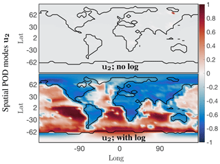
Figure 4 Dominant spatial mode 2 at the surface for the NO absolute concentration preprocessed data before and after taking a logarithm of the preprocessed data. Taking a logarithm scales the preprocessed data so that the corresponding spatial modes exhibit the global low-dimensional features, instead of only picking up on the dominant chemistry in one localized region.

Normalization of data is a common practice in data science. Indeed, the ubiquitous PCA analysis requires that each measurement type in the data have mean zero and unit variance. If this is not enforced, then those signals that are measured with large numbers will simply drown out the signals measured in small numbers. Thus, the units of the different measurements are neutralized by requiring a mean zero and unit variance. Similarly here, the large spike in the data is so large that the rest of the data are like noise comparatively. By normalizing with the logarithm, a more balanced global view of the chemistry dynamics can be extracted from the modal structures.

4.2 Modes from randomized SVD

We begin by considering the singular value spectrum and the dominant four temporal modes from the randomized SVD of the absolute concentration of O₃ (O₃). These are presented in the top panel of Fig. 5. The amount of energy explained by the most dominant singular values gives a good indication regarding the low-rank nature of the underlying data. Figure 5a shows the cumulative energy explained by the 150 most dominant singular values, as derived from randomized SVD. If all 2.7×10¹¹ model output data points were perfectly independent, each singular value would represent $\mathrm{1.0}/\mathrm{2.7}\times {\mathrm{10}}^{\mathrm{11}}=\mathrm{3.7}\times {\mathrm{10}}^{-\mathrm{10}}$ % of the total energy. Instead, we find that the first 4 singular values combined explain 97 % of the total field energy, and the first 150 singular values capture almost 100 % of the total energy. Thus, it is possible to explain 99 % of the spatiotemporal structure of the highly complex O₃ field with just 20 modes. These modes reveal many of the dominant features of atmospheric O₃. Figure 5b illustrates the structure of the four dominant temporal modes. The most dominant mode (blue line) has a flat temporal structure, i.e., its importance is independent of the time of the year. The next three dominant modes all have distinct temporal patterns, i.e., they capture periodical features of atmospheric O₃. Modes 2 and 3 (red and yellow, respectively) both exhibit a frequency of 1 year, capturing features occurring on an annual basis. The fourth most dominant mode (purple) has a frequency of 6 months. Geophysical interpretation of these modes is easiest when combining the temporal pattern with the corresponding spatial features, the latter of which are shown in Fig. 6. Shown are the spatial pattern of the eight most dominant modes for the surface. It should be emphasized that the spatial patterns change with altitude, as illustrated in the Supplement. Surface O₃ exhibits distinct seasonal patterns, which are captured by the first four modes: the first mode (top left panel in Fig. 6) resembles the annual average surface concentration of O₃. It can be interpreted as the time-invariant “average O₃” field from which all other modes add or subtract to describe the spatiotemporal variability of O₃ in greater detail. The second singular value (top right panel) shows a strong gradient at the Equator as well as a distinct urban pattern over the Northern Hemisphere (NH). The seasonal variability of this mode (peaking in August, see Fig. 5) broadly follows observed O₃ burdens in the Southern Hemisphere (SH) (Cooper et al., 2014), and O₃ is known to increase during summertime in urban areas in the NH as a result of increased photochemical activity. Singular mode 3 can be seen as an additional “forcing” to this seasonality for NH O₃: it shows dominant features over polluted areas (Europe and East China) and its seasonal amplitude complements that of singular mode 2. The most distinct feature of mode 4 is the strong pattern over Africa. We interpret this as biomass burning signal. This is supported by the frequency pattern of this mode, which shows two peaks in January–February and July–August, which is in agreement with the two biomass burning seasons over Africa (Roberts et al., 2009).

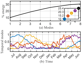
Figure 5 Cumulative energy spectrum (and inset detail) of the singular value decomposition (a) and the corresponding four dominant temporal modes (b) for the O₃ absolute concentration preprocessed data.

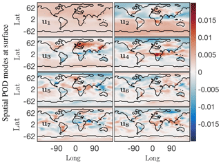
Figure 6 First eight dominant spatial modes at the surface for the O₃ absolute concentration preprocessed data. Mode 1 is the constant or mean value mode, its corresponding temporal behavior is the blue trend in Fig. 5b. Global low-dimensional spatial features for this chemical species are exhibited in order of dominance in modes 2 through 8.

To summarize, inspection of the spatial and temporal patterns of the dominant modes of O₃ shows that randomized SVD successfully reveals prominent features of tropospheric O₃ chemistry, such as elevated summertime O₃ over polluted urban areas or the two biomass burning seasons over Africa. While the data set used in this study is too short to generalize the findings, these results demonstrate the potential of randomized SVD for pattern discovery of atmospheric chemistry model output. In particular, the extent and temporal variability of the singular values can help identify highly correlated “chemical domains” within the model, which has practical applications for model reduction considerations.

4.3 Modes from randomized NMF

A drawback of the SVD solution presented in Sect. 4.2 is that it accepts both negative and positive solutions, which can result in physically unrealistic negative species concentrations. As discussed in Sect. 3.3, positive solutions can be enforced using NMF. The results from NMF for the O₃ absolute concentration data are presented in Figs. 7 and 8. The cumulative energy spectrum exhibited in Fig. 7a shows a much slower decay than the spectrum from the SVD decomposition. This is to be expected, as NMF computes an additive parts-based representation of the low-order features in the data, which preserves sparsity in the data but requires more modes to capture the same level of energy compared with the SVD. The four dominant temporal modes are presented in Fig. 7b. These now capture approximately 20 % of the total energy spectrum, compared with 97 % for the SVD. This is, in large part, due to the fact that the positivity-constraint prevents the NMF from creating a mode for annual mean O₃ that can explain most of the energy spectrum – akin to mode 1 for SVD – but that requires both additions and subtractions from this mean field to describe O₃ variations in more detail. As a result, none of the NMF modes reflects a distinct representation of the global average O₃ field. This is supported by the lack of a time-invariant mode (see Fig. 7) and also becomes apparent from the corresponding spatial patterns shown in Fig. 8. None of those resemble the average mean O₃ concentration field as, e.g., SVD mode 1 (see Fig. 6). Still, the first four spatial and temporal modes of NMF reflect some well known features of O₃ chemistry, albeit less obvious than for SVD. The most dominant NMF mode shows a pattern comparable to the second mode of SVD, and also has an almost identical temporal structure with a distinct peak in July–August. The second mode is almost a mirror image of the first mode, with a strong, broad-based signal in the NH that is most dominant during March–May but that also contributes during most other months except January. Mode 3 peaks during September–October but contributes meaningfully until February. Its spatial pattern is strongest over South America, India, eastern China, and southern Africa, and thus captures some of the increased O₃ concentrations due to fire activities (e.g., the South American burning season in August–September–October and the Indian burning season in October–November). Mode 4 is similar to mode 3 of the SVD, with strong signals over Europe and eastern China that peak during boreal spring.

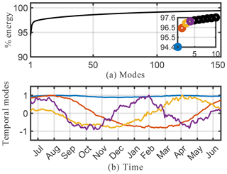
Figure 7 Cumulative energy spectrum from the nonnegative matrix factorization (a) and the corresponding first four columns of the ordered H temporal factor for the O₃ absolute concentration preprocessed data (b).

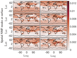
Figure 8 First eight columns of the ordered W spatial factor from NMF at the surface for the O₃ absolute concentration preprocessed data. These modes lend themselves to easy interpretation; the most dominant mode w₁ indicates that the O₃ absolute concentration is most active near eastern coastal urban China, North America, and the western coastal African continent around the region of Congo.

Similar to SVD, the spatiotemporal modes of surface O₃ derived from NMF reveal many of the characteristics of O₃ chemistry, such as increased O₃ concentrations over urban areas and biomass burning regions, as well as the seasonality of these events. Due to the strict positiveness of the solution, the signal is more muted than SVD, and significantly more modes are needed to reproduce the spatiotemporal pattern of O₃ in detail. This makes SVD better suited for off-line pattern discovery applications. However, for the practical employment of reduced-order modeling techniques within an Earth system model, we consider NMF to be superior as it still realistically captures O₃ patterns with relatively few (tens of) modes but its concentrations are guaranteed to be positive.

4.4 Modes from randomized SPCA

Spatial modes computed from the randomized SPCA are shown in Fig. 10. Note the localized features isolated by SPCA in these dominant spatial modes compared with the modes computed by the full SVD. We impose the sparsity regularizer given by Eq. (30) with $\mathit{\alpha }=\mathrm{1}\times {\mathrm{10}}^{-\mathrm{4}}$ and $\mathit{\beta }=\mathrm{1}\times {\mathrm{10}}^{-\mathrm{12}}$. Reducing the value of α gives a less sparse decomposition. The cumulative energy spectrum in the top panel of Fig. 9 again demonstrates much slower decay than the SVD and more modes are needed to capture the same amount of energy due to the sparsity constraint. In terms of energy explained and interpretability of the modes, the SPCA results for O₃ sit in between the results for SVD and NMF discussed above. The first four SPCA modes capture more than 50 % of the total energy (Fig. 9), which is more than NMF but significantly less than SVD. As for NMF, the lower amount of energy compared with the SVD can be attributed to the fact that the SPCA does not compute a dominant mode for the mean annual O₃ concentration. This is expected as SPCA is designed to capture spatially distinct features, rather than broad-based patterns. Thus, it “assembles” total O₃ concentrations from a series of modes that all show distinct spatial features. Of the dominant four modes shown here, the fourth mode most closely resembles a generic mean concentration field that contributes to the signal throughout the year (even though the signal is stronger during boreal winter). The SPCA reveals many features that are also apparent in the SVD and NMF results. The SPCA mode 1 is almost identical to mode 2 of SVD, both in spatial extent and its temporal variability. Mode 2 acts to lower O₃ over Europe and eastern China, but at a muted rate during March–May and also July–August. Therefore, it has a similar effect to mode 3 of the SVD, but with the opposite sign. Mode 3 can be interpreted as a biomass burning signal, with its distinct hot spot over Africa and the two seasonal peaks.

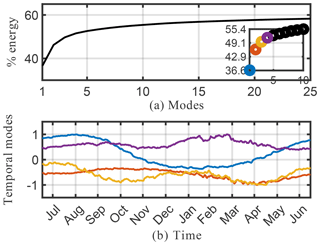
Figure 9 Cumulative energy spectrum from the sparse principal component analysis (a) and the corresponding four dominant temporal modes (b) for the O₃ absolute concentration preprocessed data.

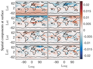
Figure 10 First eight principal components from SPCA at the surface for the O₃ absolute concentration preprocessed data. With the sparsity constraint these spatial modes exhibit only localized low-dimensional features compared with those from the SVD of the data. Compare the SVD mean value mode 1 u₁ from Fig. 6, which exhibits a more or less constant field as the dominant low-dimensional global feature, with SPCA mode 1 w₁ here, which picks up on localized dominant features in the data. The corresponding temporal SPCA mode 1 also exhibits a seasonal variation.

5 Data compression and reduced order modeling

Scalable diagnostic analysis is only one critically enabling aspect of the randomized decomposition methods. Indeed, the various randomized algorithms can be used to compute low-rank embeddings of the data that can be used for data compression. Thus, an accurate approximation of the data can be stored with a fraction of the memory requirements of the full, high-fidelity simulation. Compression is exploited in most portable electronic formats (e.g., smart phones) by representing the data using a basis which is amenable to a sparse representation (Kutz, 2013). For instance, images can be massively compressed using wavelet or Fourier basis elements as natural images are sparse in these basis elements. Compression formats such as JPEG2000 are critically enabling for the electronics industry and allow for electronic devices to hold an exceptionally large number of video, audio, and image files.

Specifically, the compression advocated here is achieved by producing a low-rank representation for constructing the high-dimensional data, i.e., it should not be confused with standard data compression algorithms. The scalable decomposition methods advocated in this paper simply require a fraction of the data to be stored in the Q matrix and the rank-r embedding columns of $\stackrel{\mathrm{̃}}{\mathit{U}}$, Σ, and V.

As an illustrative example, Fig. 11a shows a reconstruction of the absolute concentration of surface O₃ at a randomly selected time using the first 5, 50, and 100 of the SVD modes, respectively, as computed from the randomized algorithm. These reconstructions only require the storage of 0.025 %, 0.25 %, and 0.5 % of the data, respectively, as opposed to the 87 million data points of the original annual surface O₃ data (see Fig. 11b). The reconstruction with as few as five modes already shows that the dominant features are readily captured. It is also noted that there is virtually no difference between using 50 and 100 modes. The compression of the data with r modes can be computed from the first r columns of the U and V matrices along with the first r diagonal terms of Σ. This gives a data compression ratio of $(m\times n)/(m\times r+r\times n+r)$ (see Fig. 3). The compression ratio is over 4000 for 5 modes, and approximately 200 for 100 modes.

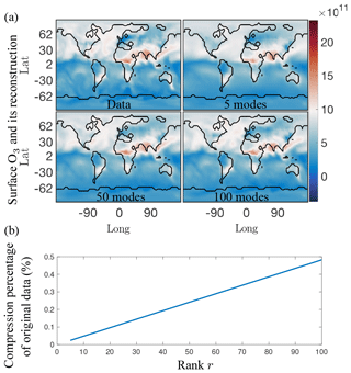
Figure 11 (a) Single snapshot of the surface O₃ absolute concentration reference data (top left) and its reconstruction using 5, 50, and 100 SVD modes, respectively. Using five modes, only the most dominant features are reconstructed successfully, but as the number of modes used for reconstruction increases more of the finer local features in the original data are picked up. Similar results hold for both SPCA and NMF. (b) Compression percentage of the original data (%) as a function of the rank of the modes retained. For the 5, 50, and 100 modes illustrated in (a), the data can be compressed into as little as 0.025 % for five modes, and 0.5 % for 100 modes.

This simple example shows that the compression of modes using our randomized architecture can serve as a critically enabling tool for the storage of numerical simulations and atmospheric chemistry data, with compression rates of up to a thousand fold. This allows the real-time analysis of simulations and data sets to be performed on laptop level computing platforms. Moreover, data can be much more easily shared for collaborative purposes as file sizes can be compressed from a terabyte to only a few hundred megabytes (5 modes) to a few gigabytes (100 modes). Such compression allows the data to be easily stored and shared on USB thumb drives.

In addition to data storage and diagnostics, the low-rank embedding spaces computed in our scalable algorithms can be used for projection-based reduced order models (ROMs) (Benner et al., 2015). ROMs are an important emerging computational framework for solving high-fidelity, complex systems in computationally tractable ways. ROMs are especially useful for enabling Monte Carlo simulations of high-dimensional systems that have stochastic variability, such as turbulent flows. The ROMs enable computation of statistical quantities like lift and drag in turbulent flows at fraction of the computational cost. Indeed, Monte Carlo computations of many high-dimensional problems of interest are currently intractable even with supercomputers; this highlights the need for proxy models that can be computed at a reduced cost. In future work, we will aim to develop ROMs that exploit the low-rank embeddings computed with our scalable algorithms.

6 Conclusions

Global environmental monitoring is becoming realizable through modern sensor technologies and emerging diagnostic algorithms. Despite tremendous advances and innovations, the data collection process can quickly produce volumes of data that cannot be analyzed and diagnosed in real-time, especially for applications like global atmospheric chemistry modeling which must integrate knowledge on hundreds of chemical species across a global longitude, latitude, and elevation grid. This emerging big data era requires diagnostic tools that can scale to meet the rapidly increasing information acquired from new monitoring technologies which are producing more fine-scale spatial and temporal measurements. We demonstrate a new set of diagnostic tools that are capable of extracting the dominant global features of global atmospheric chemistry dynamics. Not only are the methods scalable for both current and future sensor networks, they also have critical innovations allowing for improved interpretability, feature extraction, and data compression.

As demonstrated in this paper, emerging randomized linear algebra algorithms are critically enabling for scalable big data applications. The randomized algorithms exploit the fact that the data itself has low-rank features. Indeed, the method scales with the intrinsic rank of the dynamics rather than the dimension of the measurements/sensor space. Analysis of global atmospheric chemistry data shows that low-rank features indeed dominate the data. Thus, full spatial mode structures can be extracted (longitude, latitude, and elevation). This is in contrast to standard PCA reductions which do not scale well with the data size so that one is forced, due to computational constraints, to only analyze the data at fixed spatial features, such as only looking at a certain elevation. Alternatively, one can think of the scalable methods as being critically enabling for producing real-time analysis of emerging, streaming big data sets from the atmospheric chemistry community. Moreover, the dominant features of the data can be used for an efficient compression of the data for storage or reduced order modeling applications. Randomized tensor decompositions (Erichson et al., 2017b; Battaglino et al., 2018) are also viable for producing scalable diagnostic features of the global chemistry data. However, for the specific data considered here, little or no improvement was achieved. Nevertheless, in future work, we will consider such tensor decompositions across space, time, and chemicals where the randomized tensor decomposition is ideally suited for extracting higher-dimensional features.

An important aspect of this work is that simulation data, through the GEOS-Chem model, can be used to approximate the dominant global patterns of spatiotemporal activity for individual chemicals, a collection of chemicals, or the entire chemical space. The spatiotemporal features extracted provide new possibilities for understanding the interaction dynamics and relevant spatial regions where various chemical dynamics are important. This gives new possibilities for scientific discovery and the understanding of the complex processes driving the global chemistry profile.