the Creative Commons Attribution 4.0 License.
the Creative Commons Attribution 4.0 License.
 | 21 Dec 2018
TPVTrack v1.0: a watershed segmentation and overlap correspondence method for tracking tropopause polar vortices
Nicholas Szapiro
Steven Cavallo
A new free modular software package is described for tracking tropopause polar vortices (TPVs) natively on structured or unstructured grids. Motivated by limitations in spatial characterization and time tracking within existing approaches, TPVTrack mimics the expected dynamics of TPVs to represent their (1) spatial structure, with variable shapes and intensities, and (2) time evolution, with mergers and splits. TPVs are segmented from the gridded flow field into spatial objects as restricted regional watershed basins on the tropopause, described by geometric metrics, associated over time by overlap similarity into major and minor correspondences, and tracked along major correspondences. Simplified segmentation and correspondence test cases illustrate some of the appeal, sensitivities, and limitations of TPVTrack, including effective representation of spatial shape and reduced false positive associations in time. Tracked TPVs in more realistic historical conditions are consistent in bulk with expectations of life cycle and mean structure. Individual tracks are less reliable when discriminating among multiple overlaps. Modifications to track other physical features are possible, with each application requiring evaluation.
- Article
(5354 KB) - Full-text XML
- BibTeX
- EndNote


Among the disturbances on the extratropical tropopause, tropopause polar vortices (TPVs) are common coherent upper-level potential vorticity anomalies with typical radii of 100 to 1000 km and lifetimes of days to months (Hakim, 2000; Hakim and Canavan, 2005). TPV-like features play documented roles in so-called potential vorticity thinking (e.g., Holton and Hakim, 2013; Hoskins et al., 1985), surface cyclogenesis and high-impact weather (e.g., Davis and Emanuel, 1991; Grams et al., 2011; Morgan and Nielsen-Gammon, 1998; Simmonds and Rudeva, 2012), geographic climate (e.g., Kew et al., 2010; Nieto et al., 2008; Shapiro et al., 1987), stratosphere–troposphere exchange (e.g., Sprenger et al., 2007), potential predictability (e.g., Provenzale, 1999), and evaluation of model skill (e.g., Béguin et al., 2012). Knowledge of where a TPV is, how it is shaped and changing, and what it is near may aid further systematic and reproducible approaches in these and more areas. For example, TPV tracks can aid a mechanistic understanding of how information from distant radiosonde observations can impact the development of a surface cyclone days later (Yamazaki et al., 2015). Additionally, can an individual long-lived TPV contribute a significant circulation on seasonal scales? Accurate automated tracking of TPVs in gridded data improves our knowledge of TPV structure and history. Within a framework of Ertel's potential vorticity (Hoskins et al., 1985; Pedlosky, 2013; Rossby, 1939) in a composite sense (Cavallo and Hakim, 2010), dynamics of TPVs are dominated by quasi-horizontal advection subject to generally smaller diabatic and frictional forcings. Diagnostic trajectories and prognosed scalar transport further support the advection-dominated dynamics for individual cases (e.g., Sect. 3.2.1).
Tracking approaches for various features follow an approach of spatial identification and time correspondence (Hodges, 1999; Limbach et al., 2012; Neu et al., 2013; Shields et al., 2018; Ullrich and Zarzycki, 2017). However, choices and details within and among approaches can lead to systematic differences and uncertainties in results, from both algorithm sensitivities and the dynamics of the feature. For tropical cyclones, sensitivities to thresholds for size, wind speeds, warm cores, genesis, and duration impact track statistics (Horn et al., 2014; Walsh et al., 2007). For extratropical surface cyclones, deeper and stronger features are more consistent and robust across methods (Neu et al., 2013; Tilinina et al., 2013). Differences in tracks across algorithms, especially for features without independent or consensus definitions like TPVs, complicate use and interpretation as each approach is perfect within its own circular definition (Neu et al., 2013). Because our primary interest is in the physical TPVs rather than the tracked objects, clarity in the characteristics of each algorithm may lend confidence and rationale for informing whether results derived from automated tracks are artifacts or physical, especially if an ensemble with complementary approaches can be constructed by opportunity (e.g., Tebaldi and Knutti, 2007) or design.
Towards such a usable description of TPVTrack, Sect. 2 frames TPV tracking approaches and describes the current algorithm design and implementation. Idealized segmentation and correspondence test cases with reference truths quantify some of the appeal, sensitivities, and limitations of components of TPVTrack, including relative to several existing approaches (Sect. 3.1). Individual and aggregated historical cases relate the tracked objects to physical expectations of TPVs (Sect. 3.2). Section 4 concludes with a summary and possible extensions to other features.
Synoptically, we propose a functional, qualitative definition that TPVs are coherent anomalies on the dynamic tropopause associated with the larger polar vortex that have a regional minimum in potential temperature and cyclonic circulation or regional maximum in potential temperature and anticyclonic circulation that last over time. Defining “coherent”, “regional”, “associated”, and “last” is fundamental to a rule-based scheme. Note that the existence of a local extremum in a continuous surface implies the existence of a closed contour about that extremum, thus consistent with a notion of vortices (rather than waves) with trapped fluid for frictionless and adiabatic flow (Hakim and Canavan, 2005).
2.1 Existing algorithms
We summarize the automated approaches we know have been used to track and characterize TPVs or similar features in terms of multiple steps: choice and preprocessing of gridded data, segmentation in space, characterization of features, and tracking in time. Several limitations of existing approaches motivated the design and implementation of TPVTrack. With further details in the references, here we focus on comparing the interdependent choices that define regional, coherent, and lasts. Defining associated with the larger polar vortex is typically a post-processing step and applicable to any set of tracks, e.g., Hakim and Canavan (2005) subset an “Arctic” category of tracks that last at least 2 days with over 60 % of their lifetimes north of 65∘ N.
Each method bases objects about extrema. Since a surface can have many local extrema, to target salient features, filtering criteria are imposed so not all local extrema are cores of objects; an extremum must be regional. For Hakim and Canavan (2005), using 2.5∘ data, any local extremum must also be an extremum within a 650 km radius. For Kew et al. (2010), background potential vorticity is calculated by averaging over a large (107 km2) area. Positive anomalies are candidate extrema, and a flow-dependent contour of smaller prescribed area (1.7×10⁵ km2) is computed about each candidate. Lesser maxima within the bounding contour of a stronger maximum are disregarded. Simmonds and Rudeva (2014) require a local extremum in the surface Laplacian and minimum concavity for saliency through a threshold (unspecified) on an area-averaged Laplacian. In effect, choices for saliency and neighborhoods are imposed filters, integral to each approach and with a number of trade-offs as is typical of filter design.
What area is associated or coherent with a regional extremum? Spatially, where is the edge of the feature? For Hakim and Canavan (2005), eight spokes are extended from the vortex core until the radial gradient in potential temperature changes sign for each. The minimum of these potential temperature values across all eight radials defines the bounding isentrope. For Kew et al. (2010), the flow-dependent contour of prescribed area also defines the feature in space. If overlap occurs between two features, the weaker anomaly shrinks to a smaller contour yielding no overlap. For Simmonds and Rudeva (2014), radius is the weighted mean distance from the core to where the Laplacian vanishes. Consider how these definitions would represent two TPVs, one physically larger than the other. For Kew et al. (2010), the area is prescribed and the same for both TPVs. For the local gradient-based methods, sensitivity to smaller-scale noise in the surface can trigger stopping criteria with resulting areas somewhat arbitrary. Note that for some approaches (e.g., point methods) spatial shape is simply an additional diagnostic, whereas other approaches may leverage the additional information (e.g., for overlap tracking).
When is a TPV the same feature as at the previous time? How long does an individual TPV last? Hakim and Canavan (2005) use a simple proximity algorithm in which a track is extended if a vortex core is within 600 km of the previous location (advected previous location for later versions). Corresponding to a maximum vortex speed of 28 m s−1, the threshold distance subjectively works for the intended polar region and is also easily reproduced. Kew et al. (2010) develop an approach akin to contour surgery, in which cells are advected forward in time by analyzed winds, and the resulting shape is from a convex hull of the destinations after exclusion of outlier locations. Significant (10 %) spatial overlap extends a track. Note that both of these extension strategies duplicate the entire history of a TPV if there are multiple matches. Simmonds and Rudeva (2014) estimate a new position of each cyclone by weighting the track's past and climatological velocities, calculate probability of associations based on distance and central pressure differences, and keep the combination of associations within candidate groups (constructed by linking all positions within a cutoff distance) that maximize the product of pairwise probabilities as tracks. As reflected in the summary above, associations in time are decisions for whether the expected evolution sufficiently matches the actual states. Defining an expected evolution can involve a range of assumptions and complexity impacting fidelity, but approaches may be related notionally. For example, using a prescribed search radius between point locations is equivalent to calculating horizontal overlap for features with prescribed shapes of disks and no transport. Comparisons are illustrated more concretely in Sect. 3.1.
2.2 Description of TPVTrack
An implementation in Python 2.7 of this algorithm supporting and tested with output from the National Centers for Environmental Prediction's Global Forecast System (GFS; e.g., Saha et al., 2010), European Centre for Medium-Range Weather Forecasts interim reanalysis (ERA-Interim; Dee et al., 2011), Weather Research and Forecasting model (WRF; Skamarock et al., 2005), and atmospheric component of the Model for Prediction Across Scales (MPAS-A; Skamarock et al., 2012) through a modular, object-oriented approach is publicly available (see code availability section). A user's guide is included with the package. The following outlines the core modules in TPVTrack. Each module outputs one NetCDF (Rew and Davis, 1990; Whitaker, 2015) file.
2.2.1 Input data
The meteorological inputs to the algorithm are gridded zonal wind, meridional wind, relative vertical vorticity, and potential temperature on the extratropical tropopause (Gettelman et al., 2011; Ivanova, 2013) over time. With no diabatic or frictional forcings, an air parcel would have fixed potential vorticity and potential temperature. With small forcings for the associated parcels, TPVs can be tracked as material eddies on the dynamic tropopause (with preferred diagnosis described in Sect. 3.2.3).
A subset of the original domain ( in radians latitude–longitude) may be specified as the domain of interest. Within the domain, values are interpreted in a finite-volume sense as areal means located at cell centers. In deriving the tropopause surface, some data sources have missing values (e.g., GFS uses a missing value if the entire column is above the potential vorticity threshold). If no additional information is available, we fill missing values in preprocessing by an iterative extrapolation from valid nearest neighbors. We do not track globally since a potential vorticity isosurface does not correspond to the tropopause near the tropics (e.g., Highwood and Hoskins, 1998). The default is to track polewards of a user-specified latitude, set to ±30∘ for the Northern Hemisphere and Southern Hemisphere as the average position of the subtropical jet stream to be inclusive of candidate TPVs. Especially since we are interested in polar regions, we treat the longitudinally duplicated north and south poles in latitude–longitude grids specially to be consistent with the finite-volume interpretation throughout the rest of the grid. Each physical pole is treated as a single polar cap with the pole neighboring number of longitude points.
To handle various data sources modularly, each is supported natively by mesh and cell classes defining the geometry and topology of the domain. The cell class provides methods for obtaining the location, area, nearest neighboring cells, and cells within a specified radius of a cell in the mesh. For example, the left neighbor of a cell in a latitude–longitude mesh with index (iLat, iLon) is (iLat, (iLon-1) mod nLon). The mesh class provides methods for the latitudes, longitudes, and areas of all cells and finding the closest cell to a point. This allows for optimizations within a unified code implementation. For example, consider finding the cell center closest to a point in a latitude–longitude grid versus an MPAS Voronoi unstructured mesh. For a latitude–longitude grid, we can leverage the underlying structure to simply find the closest latitude and longitude independently. For an unstructured mesh, the provided connectivity of cell-to-cell neighbors can be used. Starting from a guess cell, the closest cell to the point can be found by iteratively walking towards a closer neighbor until no closer neighbor is found. Both approaches involve fewer operations than a brute-force global minimum of all cells' distances to the point. Various meshes could be unified through a common background data structure (e.g., spatial quadtree), but this is not required.
2.2.2 Spatial segmentation
Segmentation maps the mesh cells to disjoint spatial objects at each time (Fig. 1). Model tropopause data contain signals on a spectrum of wavelengths, from planetary to grid scales. These scales come from both the originating model and the post-processing that interpolates to the tropopause. As illustrated in Sect. 3.1.1, robustly segmenting TPV-scale objects requires some filtering of smaller scales. Two key questions are what counts as an extremum? What area is associated with an extremum?
A value is a local minimum if none of the values of its nearest neighbors are smaller. Local maxima can be identified by searching for local minima on the negative of the surface. There are currently two options to define a regional minimum within a prescribed region (e.g., 300 km radius disk): the smallest value or the smallest local minimum. While qualifying as the smallest value requires a comparison to all other values in the region, qualifying as the smallest local minimum is a comparison only to other local minima. A minimum across the region is a stronger filter that will result in fewer objects, while only comparing to other minima permits distinct objects as long as the minima are sufficiently separate. This may be beneficial for a tropopause with undulations within a significant larger-scale gradient. The distinction vanishes for a surface with numerous local minima. The prescribed area is a fundamental user-defined filter for a scale of saliency. Alternately, basins with less than a minimum amplitude could be filtered by merging into neighbors. This option has not been explored since it precludes identifying weak-amplitude TPVs, and a reference potential temperature is needed.
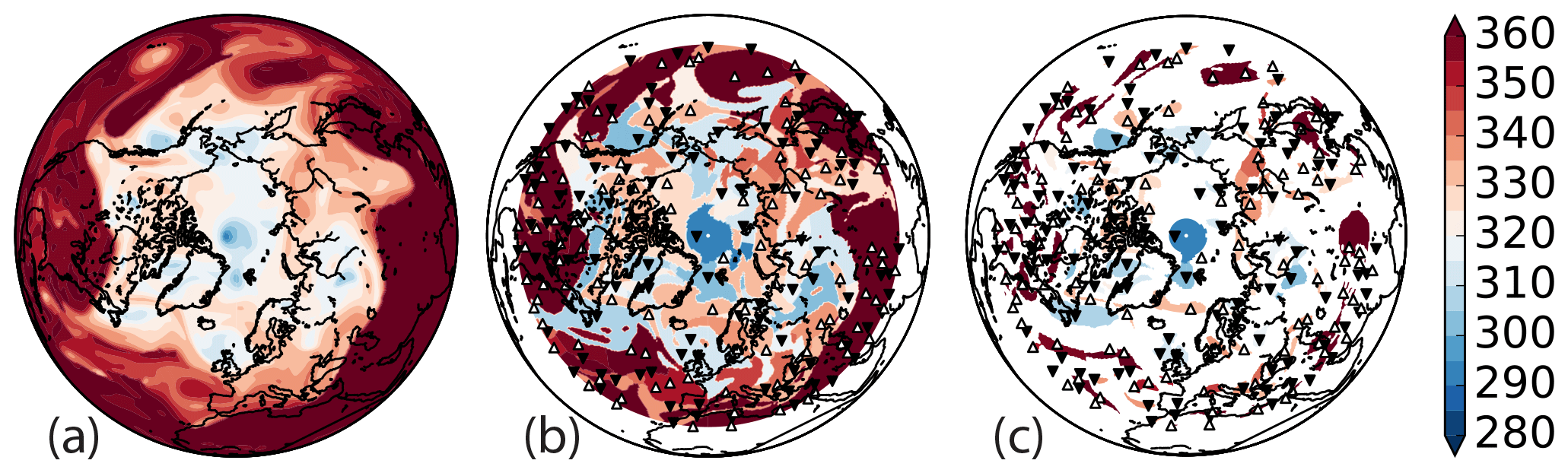
Figure 1(a) Tropopause potential temperature (K; 5 K contour interval) from ERA-Interim on 1 August 2006 00:00 UTC. (b) Segmentation into low (cyclonic) and high (anticyclonic) regional watershed basins north of 30∘ N. Regional extrema for cyclones and anticyclones are depicted by black downward and white upward triangle markers, respectively. (c) As in panel (b), with restriction within basins to the 10th percentile of boundary amplitudes.
For the area coherent with an extremum, local growing methods suffer from a noisy surface triggering stopping criteria (e.g., Sect. 3.1.1); thus a broader perspective is necessary to be more robust. Considering the tropopause as a surface with local undulations, watershed basins naturally represent the spatial objects. A watershed basin is defined by a minimum and a basin that drains by steepest descent to the minimum. Particularly given the grid-scale undulations, a direct watershed transform of the surface results in a classical over-segmentation (Serra, 1983) as each local minimum forms a separate object. To resolve the over-segmentation produced by small-scale noise, we implemented a variant of a marker-controlled watershed transform with the regional minima as markers.
The regional watershed basins are formed in two steps. First, each cell is associated with a local minimum by following a path of local steepest descent through nearest neighbors. In the case of a plateau, the cell with the smaller global index is chosen for consensus. While the occurrence of bit-equal values is rare in general, lossy data compression, idealized conditions, and other systematic factors can increase the likelihood of plateaus. Second, to form basins only associated with regional minima, each local minimum that is not a regional minimum is redirected to drain into the most intense minimum in the neighborhood, iterating until each local minimum drains into a regional minimum.
In order to segment a surface into cyclonic and anticyclonic TPVs, we first calculate watershed basins from the potential temperature surface (lows) and the negative of the potential temperature surface (highs), so each cell is initially mapped to two basins. Then, all regional extrema are mapped to themselves, and each non-extremum cell is mapped to its corresponding either high or low basin by the sign of its local relative vorticity (Fig. 1b). Thus, an anticyclonic non-extremum cell is mapped to its high regional extremum. Note that – since highs and lows are assigned based on vorticity – objects are disjoint, but each individual basin is not necessarily connected. While connectivity can be imposed by, say, flood-filling from the core of each vortex, doing so can remove filamentary substructures possibly worth preserving.
Since the resulting segmentation is driven by steepest descent of the input surface, the segmentation is sensitive to undulations in the foothills away from a vortex core. To reduce this sensitivity and better isolate the anomalies, optionally, a bounding contour can further restrict each basin (Fig. 1c). The cells outside the bound are mapped to a background. We identify boundary cells within each basin as cells with a neighbor not in the basin. A user-defined percentile (e.g., 10th) of boundary cell potential temperature amplitudes with respect to the core then sets the contour independently for each basin. A last closed contour approach (0th percentile) is noticeably less robust to outliers causing severe over-restriction, especially as the originating mesh spacing decreases (Sect. 3.2.1). Restricting the basins tends to produce smaller, more consistent objects over time. This consistency is appealing both physically and algorithmically to improve subsequent correspondence and tracking.
2.2.3 Shape metrics
The flow field associated with a TPV is expected to be related to the TPV's shape (e.g., Masarik and Schubert, 2013; Thorpe, 1986). Principally, a given idealized potential vorticity anomaly is partitioned between static stability and vorticity; a broad and shallow feature has more stability, while one that is narrow and deep has more vorticity. Moreover, the spatially larger an anomaly, the stronger the induced circulation (Hoskins et al., 1985). Towards building physical understanding and connections, various properties of a basin's geometry may be quantified by using the segmentation map of cells to objects as masks.
We organize these metrics by dimensionality: point, boundary, and area metrics. Point metrics include the latitude, longitude, and potential temperature of the core and maximum amplitude (maximum minus minimum potential temperature in the basin). Boundary cells are identified as cells with a nearest neighbor not in the same basin. Metrics include circularity (length of the perimeter with respect to the length of the perimeter of a circle with equivalent area), eccentricity (ratio of fit major and minor axes), boundary potential temperature (median of the potential temperatures of boundary cells), and boundary amplitude (difference of the boundary potential temperature from the potential temperature of the core). Area metrics are area-weighted integrals over the basin, including area, equivalent radius (of a planar disk with equivalent area), mean vorticity, and circulation. Incorporating a vertical dimension into a TPV's shape is not straightforward. A TPV's vertical extent does not extend throughout the entire column. Extending a mask on the tropopause to nearby vertical levels would need to account for the possibility of vertically tilted flow.
2.2.4 Time correspondence
Correspondences associate spatial objects among consecutive times. Motivated by the advection-dominated dynamics, the first step is to identify possible correspondences using similarity measured by “horizontal” plus “vertical” overlap. As depicted in Fig. 2, consider candidate basins A at time t0 and B at time t0+Δt.
Horizontal overlap is calculated by advecting A forward Δt∕2 and B backward in time on a sphere using the local winds at t0 and t0+Δt, respectively (Fig. 2a) (the “half-time tracking” advocated for in Hewson and Titley, 2010). We use a simple first-order scheme in which each cell center in basin A is advected on a sphere by its wind to
for latitude–longitude ϕ∕λ, zonal (u) and meridional (v) velocities, and earth radius RE. If the resulting , the trajectory has crossed a pole, and we adjust , valid for both poles. The advected location tags the closest cell as within the advected feature. B is advected back in time, and overlap occurs in the commonly tagged cells. For vertical overlap at the common time, the extreme potential temperatures of A and B are held fixed, as if adiabatic. The intersection of the potential temperature ranges is the overlap (Fig. 2b).
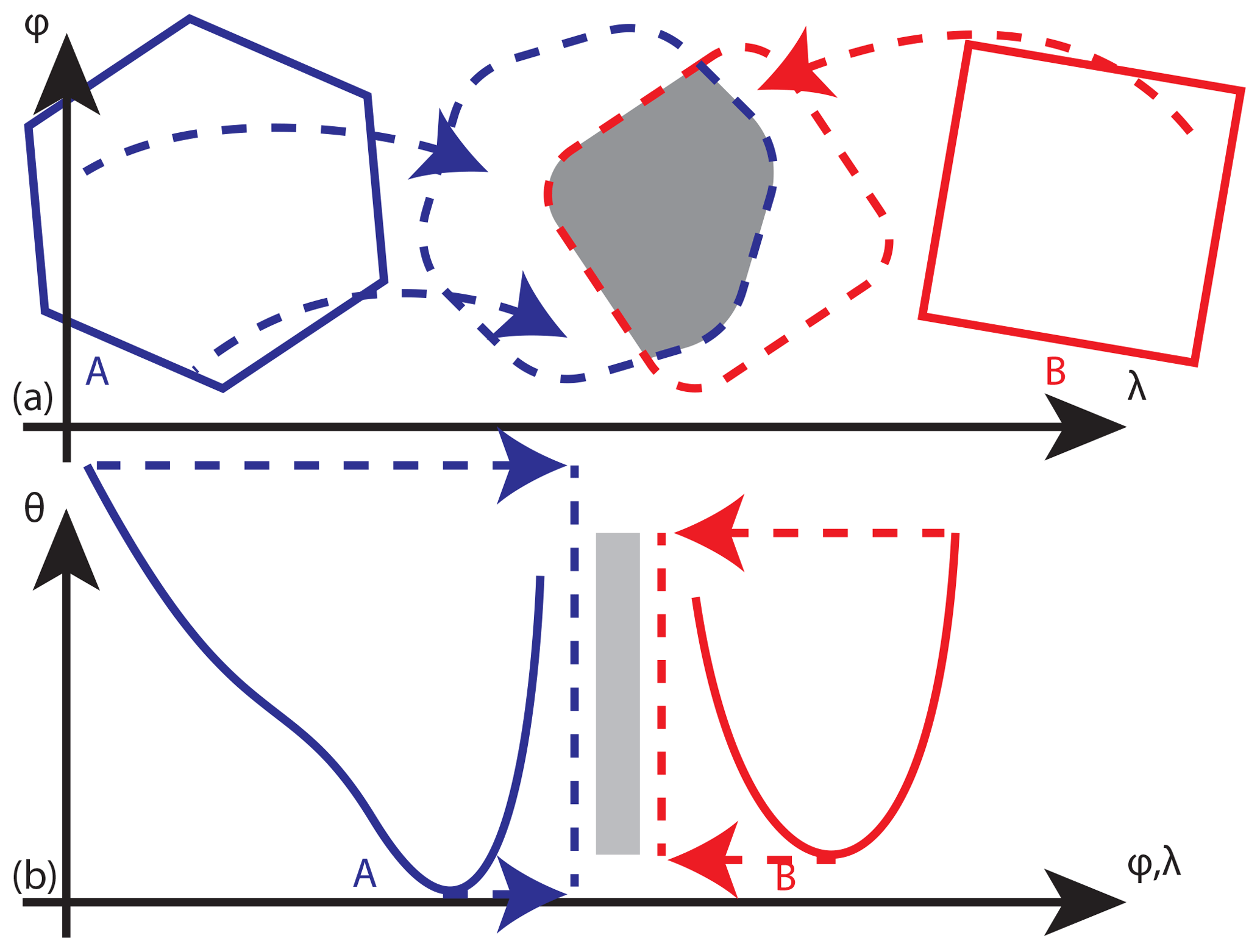
Figure 2Schematic for the (a) horizontal and (b) vertical components of time correspondence similarity quantified by overlap (gray) of a basin A at t0 (blue) and basin B at t0+Δt (red) at the intermediate half-time (dashed). (a) For the horizontal, each cell in the basin is advected, and overlap occurs in the common cells. (b) For the vertical, the potential temperature range of each basin is held constant, and overlap is the one-dimensional intersection of the ranges.
Concisely, Eq. (3) defines the similarity between basins A and B at the next time:
(where ΔΘ is the maximum amplitude) as the sum of intersections in the horizontal and vertical, respectively, normalized by the maximum possible overlap so that large areas and amplitudes are most similar to other large areas and amplitudes. Similarity is only considered for basins with horizontal overlap. Note that this also mimics how we create correspondences subjectively, in that we look for features of expected intensities in expected locations. Generically, these correspondences define candidate connections among overlapping basins and form a directed graph. Note that, technically, the t0, t0+Δt, and common correspondence grids could all be different. Such an option has not been explored but could be beneficial for time-varying or sharply nonuniform meshes.
The type of correspondence is then classified. While TPVs can form, decay, split, merge, and persist over time, we assume that a split or merger event is characterized by one primary and then secondary branches. We categorize the primary and secondary branches as major and minor correspondences, respectively. A major correspondence is a 1:1 correspondence between A and B in which both (1) B is the most similar to A of all the basins at time t0+Δt and (2) A is the most similar to B of all the basins at time t0. All other correspondences are minor.
Errors in correspondences depend on the imposed similarity function. A basin with small area or amplitude may have less chance of subsequent overlap. When there are multiple TPVs with some overlap, similarity determines major correspondences quantitatively. While we developed various alternate cost functions to define similarity based on persistence of aspects of a basin's shape over time, each basin metric has weaknesses leading to non-robust associations. For example, radius changes occur when TPVs split or merge or the basin foothills change. Intensity and amplitude can jump from data assimilation increments or strong interactions with surface lows and terrain. Practically, the inclusion of various metrics is crucial, but relative weighting requires tuning with some level of subjectivity. The (physically motivated) overlap similarity function is at least as robust for several case studies during development.
2.2.5 Time tracking
To generate tracks for individual TPVs as material eddies with histories of genesis, maintenance, and lysis, major correspondences are connected over time. A track begins when a basin has no major correspondence to a basin at the previous time and ends when a basin has no major correspondence to a basin at the next time. For example, a TPV breaking off from a parent would be tracked from the time step after the break through the chain of major correspondences. This approach avoids duplicating the entire history of a track when a TPV splits, with such repeat counting yielding inconsistencies with the actual flow state that can potentially impact subsequent composites and climatologies. To determine if a correspondence at a given time starts a track, we check whether the basin is in a major correspondence at the previous time. Without further information, all major correspondences from the initial time start tracks and to the final time end tracks. The tracks resulting from connecting major correspondences can then be further filtered as “polar” by restricting to tracks poleward of a jet stream, latitude, or other criteria depending on the application.
Here, only the major correspondences are used in forming tracks. However, the major and minor correspondences together describe a tree structure of potential overlaps of vortex air masses. For example, this tree has been used to identify all TPVs at future times that could have overlapped with specified TPVs at given times.
2.2.6 Parameter settings
To define TPVs with TPVTrack, there are four user-specified parameters: size of the filtering disk for regional extrema, percentile for watershed basin restriction, minimum lifetime, and polar classification. For the first two parameters, default settings are a 300 km filtering disk for regional extrema and the fifth percentile of the amplitudes of the basin's boundary cells with respect to the core for restriction. The scale of the filtering disk should be larger than the grid scale but smaller than a TPV. The percentile should be between (0,100) for a more robust and consistent spatial shape than using the last closed contour or the full watershed basin (Sect. 3.2.1). TPVTrack output does not depend on the latter two parameters; rather, the user imposes them in post-processing TPVs from tracks. Minimum lifetime should be chosen larger than the time interval of the input data but less than the lifetime of a TPV. TPVs are classified to be directly associated with the polar vortex if polewards of the (flow-dependent) polar jet (e.g., at genesis or during their lives).
Fundamentally, these are imposed filters, with sensitivities that can propagate through the algorithm. Increasing the radius for regional extrema generates larger basins and fewer objects. Increasing the restriction percentile will generate larger basins. Larger basins have more chance for some correspondence overlap and so may be preferentially favored to last. It is not clear how “universally optimal” settings would be defined or justified in general. The default settings subjectively best match manual tracks during several periods of interest (August 2006, July 2007, August 2012, and January 2014) in terms of track and basin shape. User-defined parameters are exposed in one settings file, and it is straightforward to vary them towards assessing sensitivities within a fixed tracking approach.
2.2.7 Computational cost and acceleration
For ERA-Interim data from 1 January 2010 00:00 UTC through 30 June 2015 18:00 UTC every 6 h, the serial version of TPVTrack takes 25.44 wall-clock hours per tracked year. Of the total run time, preprocessing, segmentation, metrics, correspondence, and tracks take 1.9 %, 78.3 %, 1.4 %, 7.4 %, and 11.0 %, respectively, including input–output. Timings are from an HP Z600 Workstation (eight Intel Xeon E5620s processors at 2.40 GHz with 11 GB of cache memory and 16 GB of RAM) with Linux version 2.6.32-504.1.3.el6.x86_64 and Python 2.7.12 from Anaconda.
To reduce wall-clock time, a number of optimizations are possible. A more efficient implementation of a discrete watershed transform leveraging sorting (Roerdink and Meijster, 2000) could be used for segmentation. While the modules are sequential, each has an embarrassingly parallel decomposition as written (with modifications to file input–output). Within the current version, preprocessing the input data is independent over time, segmentation is independent over time, calculation of metrics is independent over time, categorization of correspondences is independent over basin and neighboring times, and construction of tracks is independent over track. Each process can write separate contiguous output files that are then concatenated into one file to maintain consistency with the serial version. Parallel versions of the segmentation and track modules have been implemented using Message Passing Interface in Python (Dalcín et al., 2008) with near-linear speedup for each component and results identical to the serial version (for four processes). The only communication among processes is global barriers between modules since the modules are sequential and output is written to file.
Does TPVTrack accurately represent and track TPVs? Ultimately, any validation (Roache, 1998) depends on a reference truth. We explore this question through both simplified component test cases with reference solutions (Sect. 3.1) and historical cases with more realistic conditions but less clear expectations (Sect. 3.2). A complete discussion, if possible, is beyond the scope of this paper. Rather, we intend the following to highlight characteristics of the approach and direct future sensitivity analyses and intercomparisons. Users focusing on case studies are encouraged to test robustness of individual tracks, while systematic artifacts may be more relevant for climatologies.
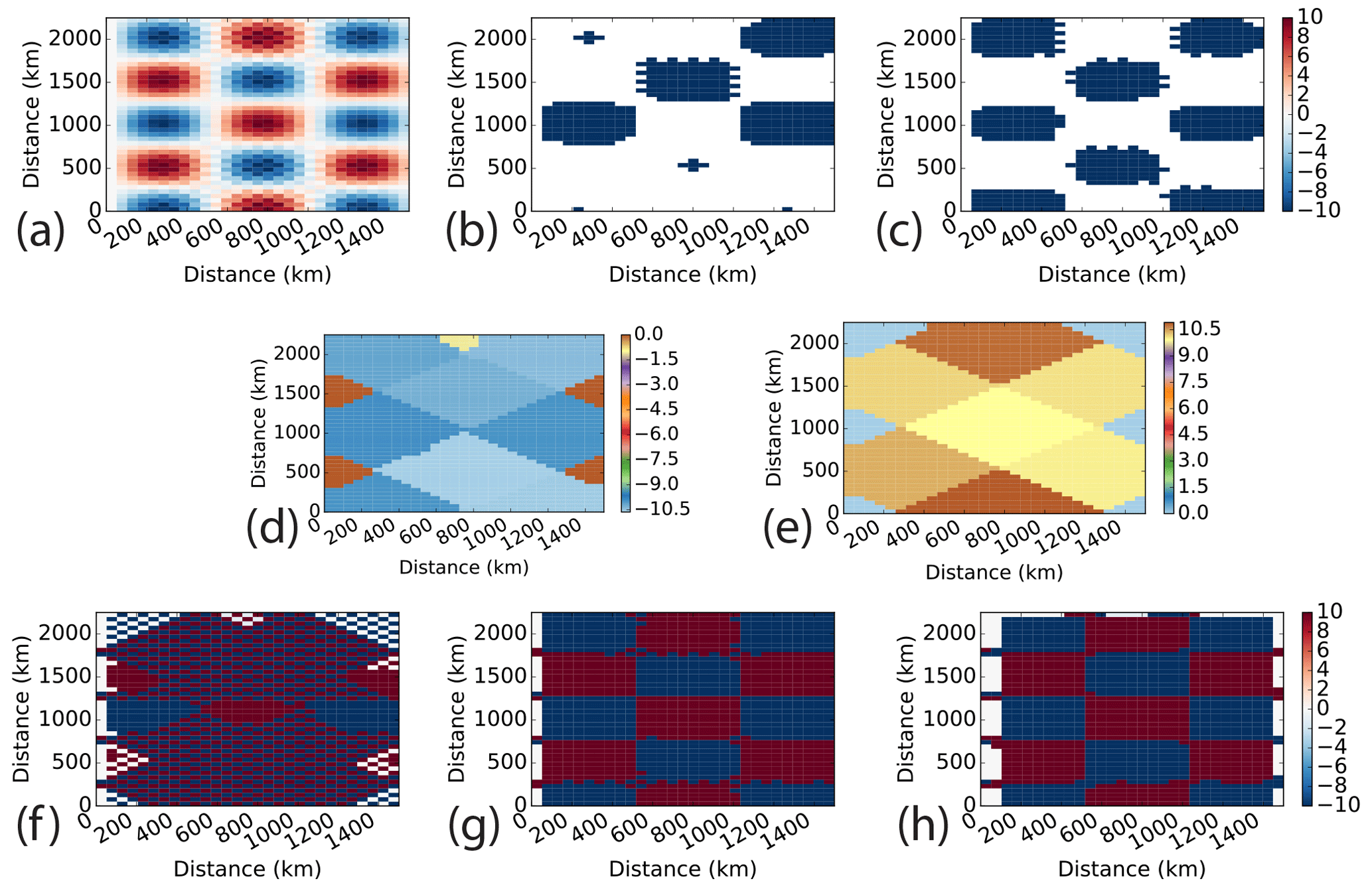
Figure 3Comparison of (b) H05, (c) K10, and watershed (f, g, h) segmentations for an analytic surface with multiple scales (a; Eq. 4). For the watershed method, each cell is in both a (d) low and (e) high regional watershed basin. Assignment to one is by the local relative vorticity, calculated by (f) centered finite differences on the raw field, (g) a smoother Gaussian–Laplacian with a standard deviation of 1, or (h) sign of the vorticity equals opposite the sign of the surface (a). Each object in a segmentation (b–h) is colored by the intensity of its core. Color bars (K) for panels (a), (b), (c), (f), (g), and (h) are the same.
3.1 Idealized test cases
Spatial segmentation and time correspondence are central to all approaches. We construct a simplified test case for each – Sect. 3.1.1 and 3.1.2, respectively – to better isolate and assess specific differences. TPVTrack is compared to our implementations of Hakim and Canavan (2005) and Kew et al. (2010) as reference point and areal methods, respectively termed H05 and K10.
3.1.1 Spatial segmentation
For segmentation, consider a surface θ (Fig. 3a) and vertical relative vorticity ζ motivated by the Sander's analytic model (Bluestein, 1992) with
where K, km, and mimic various scales of undulations, as for the tropopause (Shapiro et al., 1987). Results are depicted in Fig. 3 on a grid with 50 km spacing.
While the eight main regional lows are represented in all approaches, the shapes of the objects reflect differences in the algorithms. For H05, the gradient radially outward from the extremum first changing sign defines the bounding contour. Local noise in the surface is amplified by gradients and can drastically shrink objects (e.g., objects near versus (1400,1000) in Fig. 3b), which may be mitigated with suitable prior filtering. For K10, the maximum area of each object is prescribed (1.7×10⁵ km2), with smaller objects resulting from overlapping areas (e.g., the two y=100 objects in Fig. 3c). While the low and high watershed basins are more robust to local undulations (Fig. 3d, e) because of the regional extrema filter, the assignment of cells to objects is entirely dependent on the sign of the cell's vertical vorticity. Centered finite differences on the raw field amplify small scales not coherent with the expected larger-scale features (Fig. 3f). Reducing the small-scale noise in the vorticity (Fig. 3g) is more consistent with the larger-scale perspective (Fig. 3h).
There are also differences in the objects along x=0. For H05, the boundary values are not regional minima given the 650 km search radius. For K10, the 0.5 K contour interval we used for growing each object in turn filters the boundary local minima as parts of existing, more intense objects. For the watershed markers, the 300 km search radius yields boundary objects when aligned with the vorticity. In TPVTrack, this filtering radius is user defined.
3.1.2 Time correspondence
Consider individual disks of radius r and potential temperature range advecting about a domain with
for position (x,y), velocity (u,v), and additional noise increments σ∗. The increments σ∗ are a simple way to introduce additional time evolution and are generated independently and stochastically, with the random number generator seeded with 0 for reproducibility. During evolution, we bound r≥10 km and K. By construction, a given disk should always and only correspond to itself over time.
For the control case, we initialize 50 objects with uniform 20 km x–y spacing. The initial velocities are sampled from uniform distributions m s−1, core potential temperatures from a normal distribution K, intensities from K, and radii km, motivated by Fig. 6 in Hakim and Canavan (2005). The noise terms sample centered uniform distributions of m s−1 and K. Evolving each cell independently for 12 6 h time steps, we can consider the correspondences determined by each approach (Fig. 4). H05 and K10 create numerous false correspondences among nearby objects but miss no correspondences. The stricter 1:1 definition for major correspondences in TPVTrack greatly reduces the rate of false correspondences but yields several false negatives. Especially since the parameters for the control setup are somewhat arbitrary, several perturbations from the control have been tested. Changes to the initial separation, time step, velocity amplitudes, and noise amplitudes (not shown) also yield results consistent with the following.
The simple test case illustrates characteristics of each approach. H05 creates correspondences whenever candidates fall within a distance cutoff. K10 creates correspondences when sufficient horizontal overlap occurs under advection. Correspondences from both are less robust for multiple close objects than TPVTrack, which incorporates horizontal overlap, vertical overlap, and 1:1 major correspondences. Rather than subjectively valuing one approach as absolutely better than another, these could be considered complementary tools. Overlap is useful for identifying possibly associated features through time. Further major correspondences use additional information to provide more targeting for following a distinct individual feature.

Figure 4False positive (red) and negative (blue) time correspondence rates for the control setup of the idealized correspondence test case for H05 (dashed), K10 (dash-dotted), and TPVTrack (solid) approaches. Rates are in bins of 100 km core–core distance. For H05 and K10, false negatives are zero and false positives overlap for distances less than 600 km.
3.2 Historical test cases
The purposefully simplified segmentation and correspondence test cases permit precise reference solutions. Further evaluation using more realistic historical data centers on two questions: are TPVs tracked by TPVTrack? Are tracks TPVs? Tracks were constructed using the default settings with ERA-Interim 2 PVU dynamic tropopause data for 1979 to 2015 every 6 h. TPVs are defined as tracks with a core at genesis north of 60∘ N lasting at least 2 days. This relaxes the Arctic category of Hakim and Canavan (2005) to tracks that start polewards of the mean position of the polar jet.
3.2.1 Are long-lived TPVs tracked?
A track in 2006 is one of the longest in this dataset, from 6 July to 30 September 2006. It is of particular interest because of its long lifetime and associations with Arctic sea ice loss. Tracking manually, we can follow this TPV forming from filamentation and splitting on 3 July over western Siberia to dissipating on 30 September over eastern Siberia after traversing much of the central and eastern Arctic. The advective nature of the TPV is evident in comparing the TPV's track to a trajectory model (Stein et al., 2015). For example, 5-day forward and backward trajectories from 15 August 2006 00:00 UTC about the core using Global Data Assimilation System meteorology and model vertical velocity are near the core for the 10-day period. Using several less robust segmentation and correspondence settings, the TPV's track stops on 29 July, 3 September, 9 September, or 17 September instead. Figure 5 depicts the states driving these sensitivities. Generally, given multiple TPVs with overlap, major correspondences are discriminated quantitatively by similarity scores.
Ullrich and Zarzycki (2017) argue that a closed contour criterion is appealing since it is less sensitive to grid resolution relative to using only nearest neighbors. Here, we quantify some of TPVTrack's spatial sensitivities by segmenting an existing ensemble of full-physics, limited-area simulations with model grid spacing from 12 to 120 km. We use WRF-ARW version 3.8.1 (WRF Users, 2016) on a roughly 6000 km-by-6000 km domain centered on the North Pole with 41 vertical levels up to 10 hPa with a time step of Δt=5Δx (e.g., 600 s for 120 km). Initial conditions on 15 August 2006 00:00 UTC are from GFS analysis with lateral boundary conditions updated every 3 h from alternating GFS 6 h analyses and 3 h forecasts. Physics parameterizations include Morrison two-moment microphysics (Morrison et al., 2009), rapid radiative transfer model longwave radiation (RRTM-LW; Mlawer et al., 1997), RRTM for general circulation models shortwave radiation (RRTMG-SW; Iacono et al., 2008), the Unified Noah land surface model (Tewari et al., 2004), and the Yonsei University planetary boundary layer (Hong et al., 2006). The tropopause is diagnosed using NCAR Command Language (NCL) functions wrf_pvo to calculate potential vorticity and wrf_user_intrp3 to interpolate to 2 PVU, similar to values found by interpolating in the vertical to 2 PVU by searching down from the model top (Sect. 3.2.3) for these grid scales.
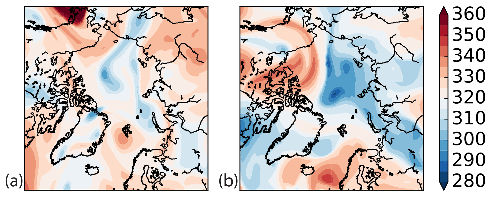
Figure 5Maps of tropopause potential temperature (K; 5 K contour interval) for dates with sensitivities in the long-lived summer 2006 track; (a) 29 July 2006 00:00 UTC; (b) 17 September 2006 00:00 UTC.
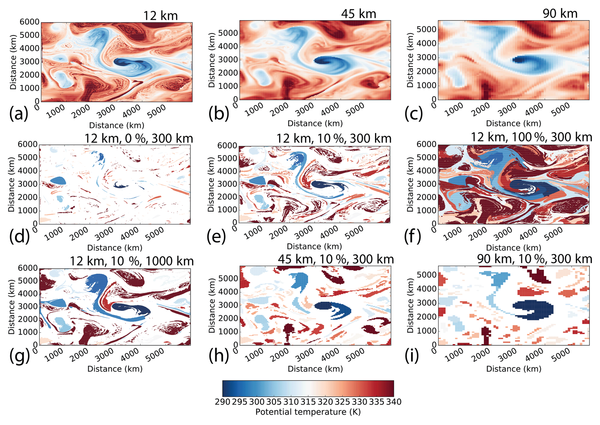
Figure 6Segmentation of (a) 12 km, (b) 45 km, and (c) 90 km WRF tropopause (after 3 simulation days) for (d) 12 km, 0 % restriction of boundary amplitudes, and 300 km regional extrema; (e) as in panel (d), but 10 % restriction; (f) as in panel (d), but 100 % restriction; (g) as in panel (e), but 1000 km regional extrema; (h) as in panel (e), but for 45 km simulation; (i) as in panel (e), but for 90 km simulation.
While the number of local extrema increases for the higher-resolution grids within the first day as the model spins up from the external initial conditions, the number of regional extrema remains nearly constant. Comparing the segmentations for the 12, 45, and 90 km grids after 3 days, there are combined effects of dynamical model and segmentation filters (Fig. 6). Simulations using higher-resolution grids have finer-scale structures (Fig. 6a, b, c) that are preserved in the segmented basins (Fig. 6e, h, i). A larger filter radius for regional extrema reduces the number of basins and generally increases amplitudes (Fig. 6e, g). Using the last closed contour over-restricts most of the basins (Fig. 6d, e, f). Note that over-restriction can be basin dependent, with the low near (1000, 3200) similar across all panels. Focusing on the long-lived 2006 TPV near (3000, 3000), the segmented basin is larger for a larger cutoff radius, boundary contour percentile, or grid spacing (Fig. 7). The r1000 0 % basin at 12 km is spuriously small. The large imposed filter generates fewer and larger regional watershed basins. The minimum potential temperature along the resulting extended boundary is near that of the core, greatly reducing the restricted extent. Vortex cores may also be near the basin's boundary dynamically, like in conditions of strong deformation. In general, the shape of the distribution of potential temperature on the boundary of the watershed basin determines the sensitivity to the restriction percentile threshold; a uniform distribution with a small range would exhibit little sensitivity.
The longest anticyclone track starts on 28 April 1979 and lasts 25 days (Fig. 8). Synoptically, a filament from an amplifying Rossby wave break over the northeastern Pacific Ocean develops into a closed feature, couples with numerous cyclones over its entry into and traversal of the Arctic, and dissipates into the polar jet stream east of Greenland. TPVTrack's track exactly matches our manual track.
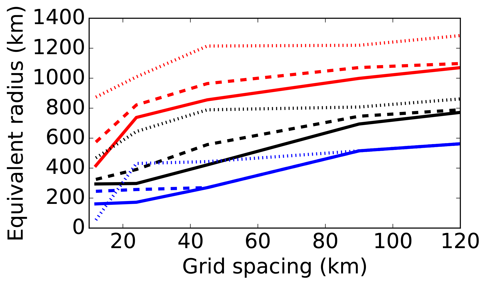
Figure 7Equivalent radius of long-lived 2006 TPV from watershed segmentation of 12 to 120 km WRF simulations (at 3 days) with 300 (solid), 500 (dashed), and 1000 km (dotted) regional extrema and basins restricted to 0 % (blue), 10 % (black), and 100 % (red) boundary amplitudes.
3.2.2 Bulk evaluation of tracks
Case studies are central to the iterative development of TPVTrack. A common sensitivity, as in the summer 2006 example, occurs when TPVs highly deform or intensify while in a neighborhood with multiple candidate overlaps. Beyond case studies and estimating skill through verification against a limited set of subjective and questionably reproducible manual tracks, bulk statistics can be used to evaluate methods (Lakshmanan and Smith, 2010). What are the characteristics of tracked TPVs? Are these consistent with expectations? Note that a TPV climatology is beyond the scope of this paper and is the focus of a separate work.
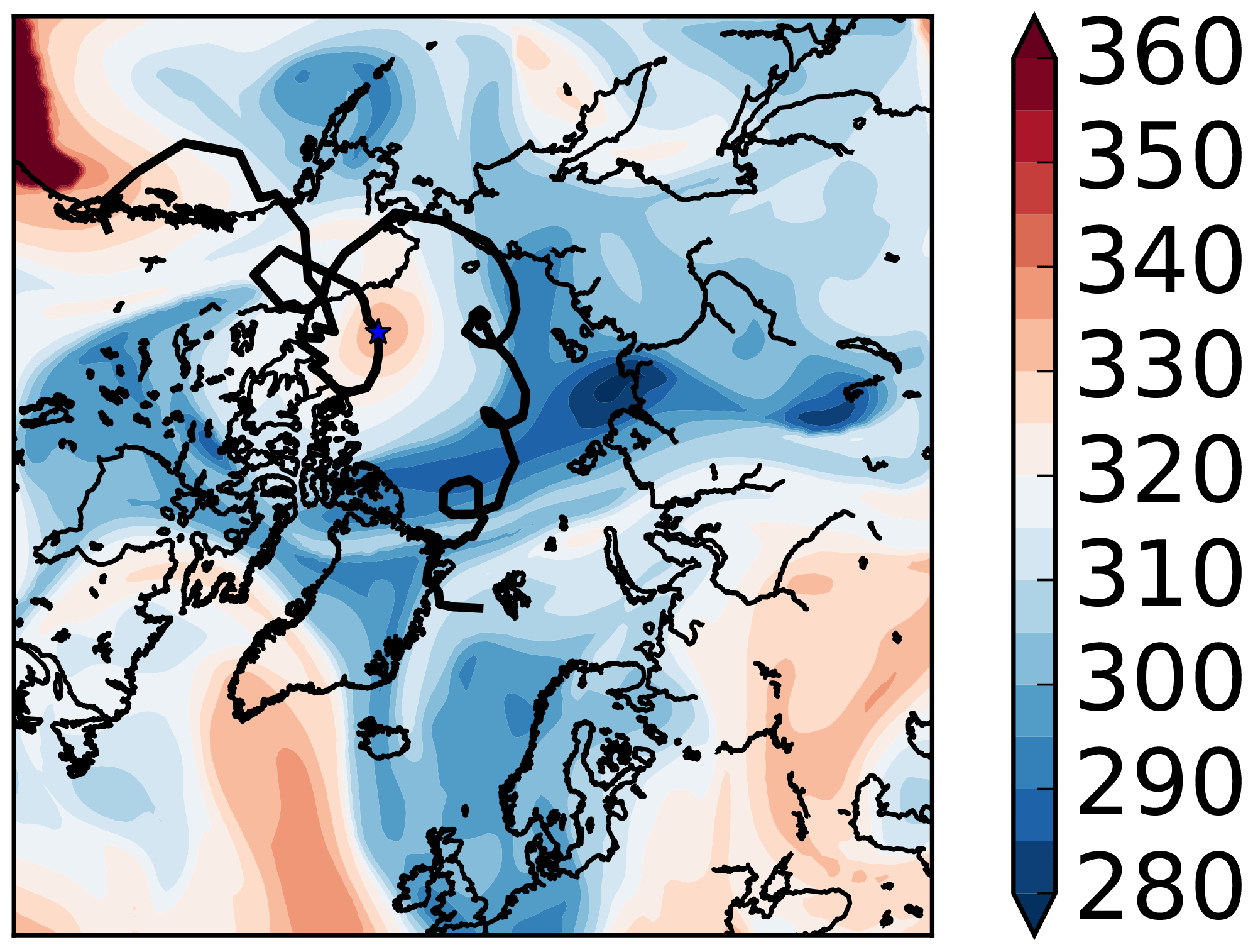
Figure 8For the longest anticyclone track in 1979 to 2015, a map of dynamic tropopause potential temperature (K; 5 K interval) at 3 May 1979 00:00 UTC and track of the core overlaid in black. The location of the core (north of Alaska) is starred at the common time.
While a fuller understanding of the life cycles of TPVs is a matter of ongoing research, Hakim and Canavan (2005) show TPVs to be generally smaller in radius at genesis or lysis in comparison to the rest of their lifetimes. Both cyclonic and anticyclonic tracked TPVs reach their minimum radius at the beginning or ends of tracks in the majority of cases (Fig. 9). The tail-dense distributions are also similar for time of minimum amplitude and circulation (not shown). The maximum radius tends to occur between genesis and lysis (not shown). Tracks with a larger maximum radius have larger maximum circulation, amplitude, and lifetime (p<0.01).
By construction, tracked TPVs are regional lows in potential temperature with cyclonic vorticity or highs in potential temperature with anticyclonic vorticity. To evaluate TPVs spatially, the Okubo–Weiss parameter (Okubo, 1970; Weiss, 1991) W is
where , , and are normal strain, shear strain, and relative vorticity, respectively. We include additional metric terms for latitude–longitude grids treating convergence near the poles (Saucier, 1955). If relative vorticity dominates strain, W<0. Maps of W tend to exhibit three regions: rotational vortex cores characterized by negative W, strain regions surrounding vortices characterized by positive W, and background regions with small absolute W (Provenzale, 1999). For a TPV-relative reference frame, we center a cardinally oriented computational grid with uniform 30 km spacing about each TPV core. Values within tracked basins are nearest-neighbor interpolated from the original grid onto the reference grid through a stereographic projection centered on the TPV core. Given the expense of remapping following each TPV, we consider one year (Fig. 10a, b). Cyclones are frequently rotational about the core, while for anticyclones the region of concentrated rotation is less frequent, broader, and offset northwards of the core. Considering tracks with at least a 10-day lifetime yields a more rotationally dominated structure about the core (not shown). Geographically, (Fig. 10c, d), tracked cyclones tend to have negative W except near orographic features, while tracked anticyclones appear to have higher strain at lower latitudes where shear interactions with jet streams would occur.
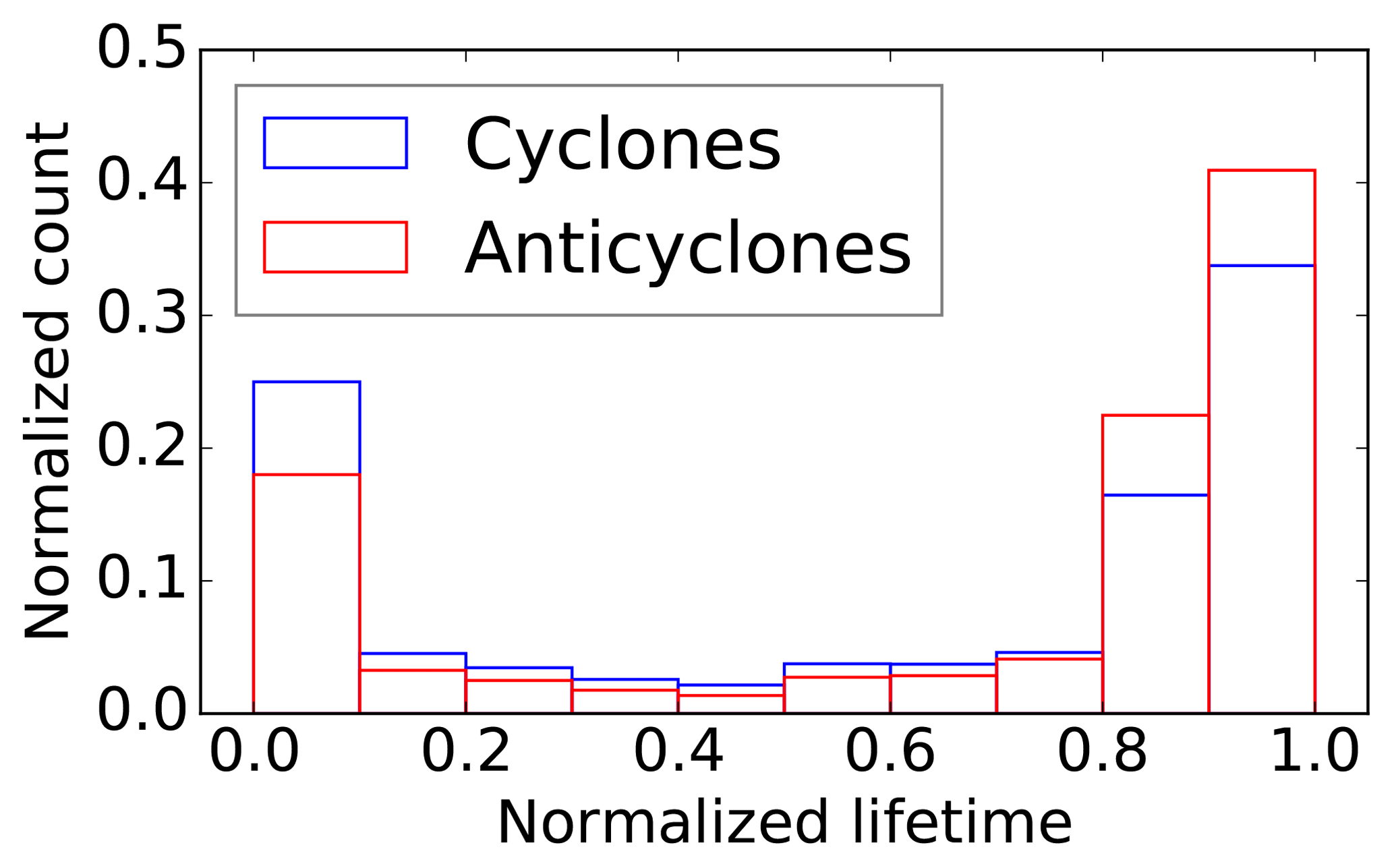
Figure 9Fraction of all cyclonic (blue) and anticyclonic (red) TPVs in 1979 to 2015 with their minimum equivalent radius as a function of stage between genesis and lysis. The normalized lifetime is linear in time between 0 at genesis and 1 at lysis within each track. The count is normalized to a fraction by the total number of TPVs (41 190 and 33 392 for cyclones and anticyclones) and aggregated in 10 equally spaced normalized lifetime bins.
Thus, in bulk, TPVs from TPVTrack are consistent with eddies with rotational cores exhibiting reasonable genesis and lysis and consistency among metrics. The symmetric, core-relative vortex structure is less frequent for features that are shorter-lived, over mountainous terrain for cyclones, or interacting with lower latitudes for anticyclones. However, it is unclear how discriminating these bulk results are. An intercomparison of trackers would further inform relative algorithm evaluation.
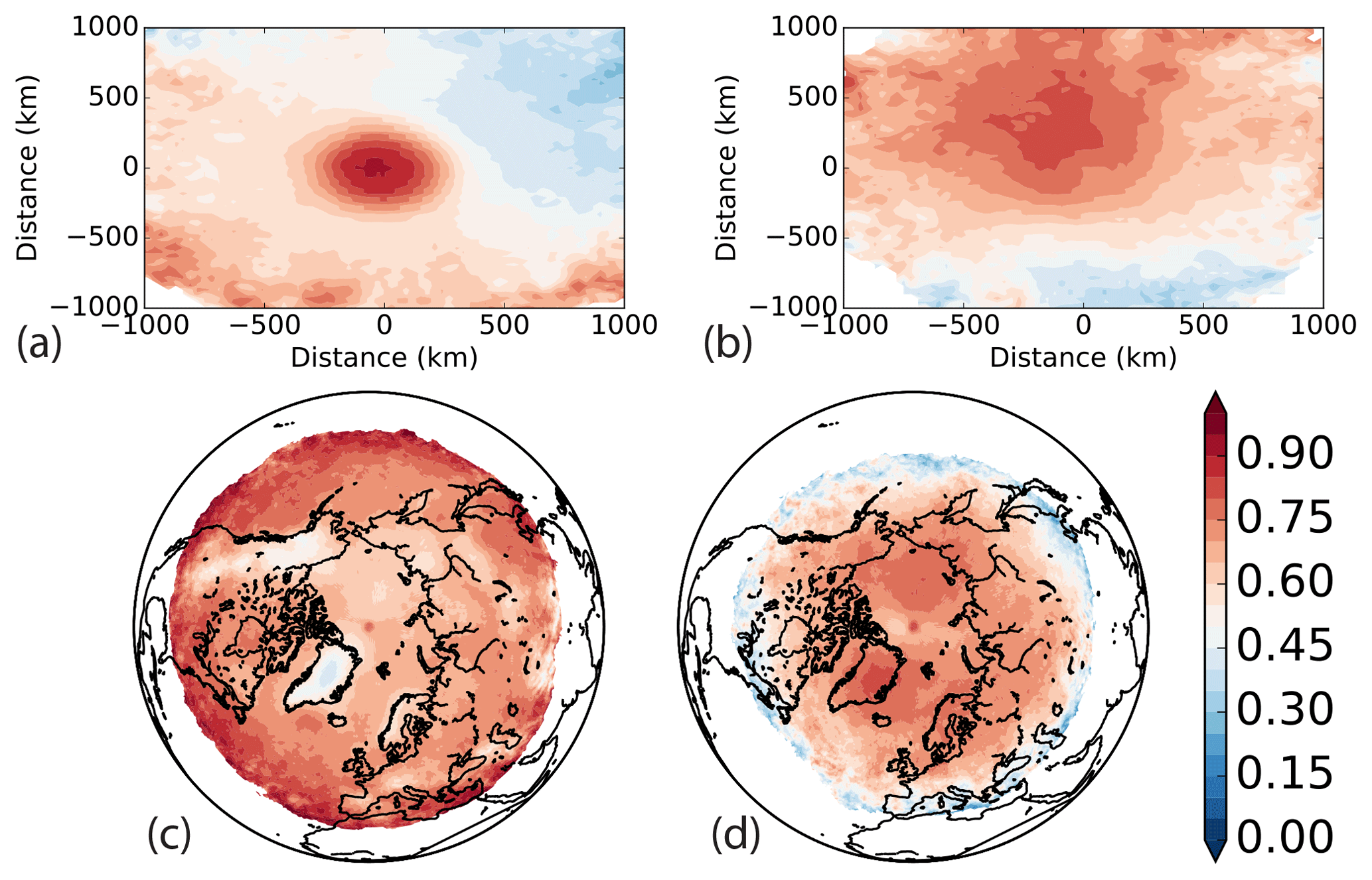
Figure 10Fraction of time with a negative Okubo–Weiss parameter given the cell is within a TPV, (a) cyclonic TPVs in 2006 in a core-relative reference frame, (b) anticyclonic TPVs in 2006 in a core-relative reference frame, (c) cyclonic TPVs in 1979 to 2015 geographically, and (d) anticyclonic TPVs in 1979 to 2015 geographically. Values with fewer than 5 days of samples (on the domain boundaries) are masked in white. The contour interval is 5 %.
Most likely occurrences of TPVs from TPVTrack in the central Arctic and Canadian Archipelago (Fig. 11a, b) are consistent with Cavallo and Hakim (2010). Varying the geographic criteria for defining TPVs from tracks yields differences of the same order as the expected density for TPVs near midlatitudes and little difference polewards (Fig. 11c). Decreasing the minimum duration required of tracks (Fig. 11d) has a relatively smaller impact, generally increasing the total number of TPVs with maximum differences broadly over the North Atlantic and European Arctic.
3.2.3 Accommodations for model data
Several practical issues have been noted through application of TPVTrack to model data, largely related to the diagnosis of the tropopause and scales of interest. Treatment of missing data via iterative flood fill (Sect. 2.2.1) is included in the code release. Especially at finer grid scales, relative vorticity may need to be filtered, similar to the noise issues seen in the idealized segmentation test case when assigning cells to either highs or lows. In computing metrics, raw or filtered fields could be used, in a trade-off of consistency with the original flow field versus scales of interest.
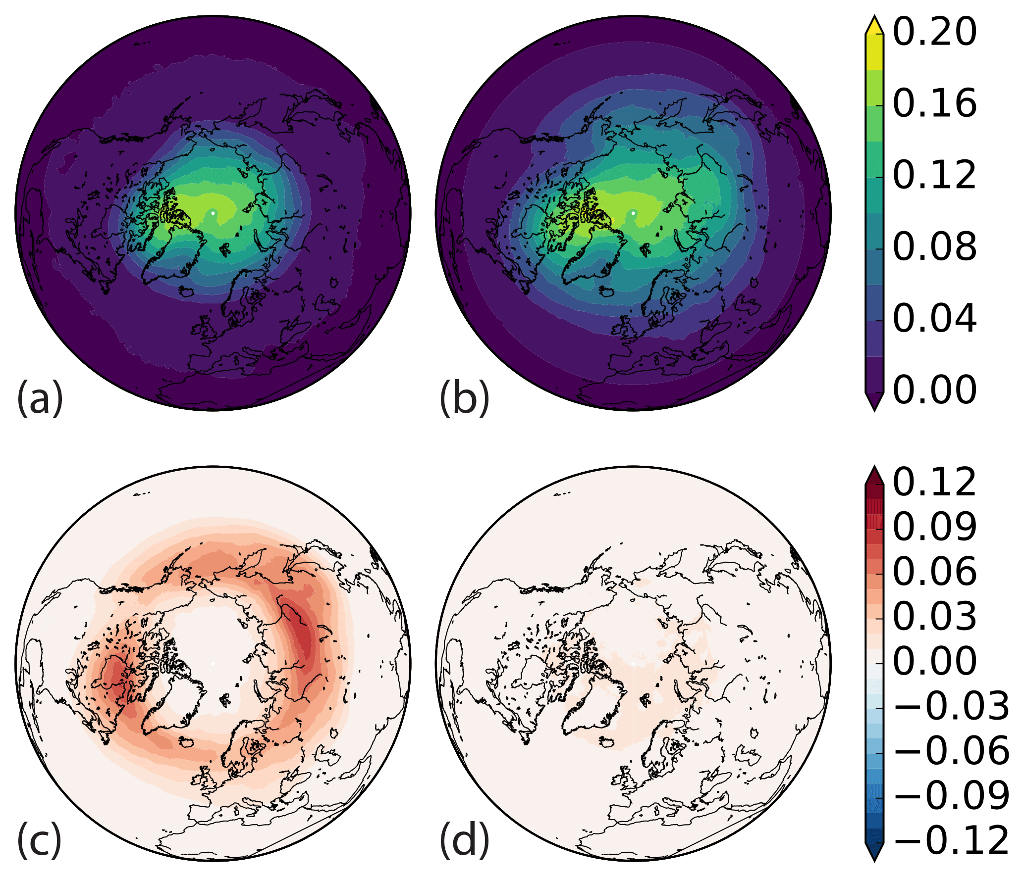
Figure 11Geographic probability of a cyclonic TPV present from ERA-Interim 1979 to 2015, calculated by aggregating times within basins of tracks satisfying TPV criteria. (a) TPVs defined via the H05 “Arctic” category, in which TPVs are tracks that last at least 2 days with over 60 % of their lifetimes north of 65∘ N. (b) Default TPVTrack settings, for which TPVs are tracks lasting at least 2 days with genesis north of 60∘ N. (c) b − a. Difference in probability using different latitude criteria for defining TPVs of genesis north of 60∘ N minus 60 % of lifetime north of 65∘ N. (d) Difference in probability using different lifetime criteria for defining TPVs of a minimum lifetime of 1 day minus 2 days. A 300 km radius for regional extrema and 5 % watershed boundary amplitude restriction apply to all. Contour intervals are 2 % for panels (a) and (b) and 1 % for panels (c) and (d).
While a dataset may define its own diagnosis of the dynamic tropopause, conventionally the dynamic tropopause is found by searching down from some upper level or model top for a potential vorticity threshold within each column independently, possibly with thickness criteria (e.g., Zängl and Hoinka, 2001). However, vertical mixing, folding, and convective-scale vorticity can generate ambiguity with multiple candidates for the tropopause within a column, occurring globally (Añel et al., 2008). Beyond thickness conditions, we have found the tropopause as a surface to be identified more robustly by including consistency with information outside the column. To identify the tropopause as a layer between the connected high potential vorticity stratosphere and low potential vorticity troposphere, flood-fill segmentations of the stratosphere and troposphere can be performed. For example, starting with initial seed cells near the surface with low potential vorticity, all connected values below a chosen potential vorticity threshold can be found by iterating through valid nearest neighbors. This identification of the connected troposphere yields the tropopause as the top of the tropospheric volume. Note that the top of the troposphere is above the bottom of the stratosphere, and the bottom of the stratosphere may reach the surface, especially within potential vorticity towers (e.g., Pang and Fu, 2017, Fig. 6c). If model data are archived with sparse vertical levels, this diagnosis may have larger uncertainties. Also note that the chosen isertelic level can impact TPV metrics quantitatively (e.g., Fig. 4 in Cavallo and Hakim, 2009).
Typical model output frequencies range from hourly to daily. The simple-advection constant-amplitude overlap similarity is less appropriate with decreasing time resolution. Tracking on under-resolved fields may increase systematic misidentifications of TPVs. Note that genesis at the initial time and lysis at the final time are not dependent on the flow field but rather on truncated time input.
TPVTrack is a software package for rule-based tracking of TPVs motivated to address limitations of spatial characterization and time tracking within existing approaches and to further our understanding of TPVs and their connections throughout the Earth system. The two primary goals are more robust representations of (1) the spatial structure of features, through restricted regional watershed basins, and (2) mergers and splits in time, through major correspondences from 1:1 similarity overlap. From the simplified test cases, robust segmentation is directly dependent on the vertical vorticity used to associate cells with cyclones and anticyclones, possibly requiring smoothing for noisy fields in preprocessing. Major correspondences reduce the false-positive associations but can increase the false-negative rate, relative to H05 and K10. Horizontal overlap may benefit from more frequent output or a more sophisticated trajectory model. Including information from more times may make tracking more robust, say with further hypothesis management (e.g., Reid, 1979). Historical test cases reveal larger uncertainties in tracks and sensitivities to user-defined parameters when multiple TPVs are in a neighborhood.
Using the default settings, TPVs are most often found over the central Arctic and Canadian Archipelago, decreasing in density with distance. In bulk, cyclone structure is frequently characterized by a rotationally dominant core, while anticyclones are less so. Cores are less rotationally dominant for shorter lifetimes, near mountains for cyclones, or near lower latitudes for anticyclones. A TPV's smallest radius tends to occur at the beginning or end of its life, while the maximum occurs between. Individual TPVs can live several months, but lifetime, size, and climatological density can exhibit sensitivities and corresponding uncertainty to input data, tracking method, and TPVTrack settings. TPVTrack has four user-specified parameters. Size of the neighborhood for regional extrema and percentile for restriction of watershed basins are specific to TPVTrack. Minimum lifetime and polar criteria for tracks are applicable to all methods. Given these sensitivities, there are concerns over use of a single approach depending on the intended application.
Further analysis is important to distinguish the TPV-related information as opposed to automated rule-based objects and whether our physical understanding is impacted. With complementary approaches, several algorithms may be combined constructively to reduce artifacts of any single approach during analysis. In addition to providing another method, TPVTrack's modular design and exposed settings file facilitate intra-algorithm sensitivity studies. Note that alternate methods for segmentation (e.g., connected anomalies of minimum intensity or size) could be incorporated within TPVTrack as different models for spatial shape, with no modifications needed for the rest of the algorithm. Perhaps more fundamentally, can a TPV have multiple centers (e.g., Hanley and Caballero, 2012)? Users focusing on case studies are encouraged to test robustness of individual tracks, while systematic artifacts may be more relevant for climatologies, including sensitivity to the input data.
The equivalent radius of a TPV's basin measures one aspect of size. Physically, the size of a TPV may refer to a number of scales, including where fluid is more trapped near the core, the (anti)cyclonic basin about an extremum, minimum distance of the core to a boundary, or the region of flow influenced by the potential vorticity anomaly. Are there clear relationships among these scales? Are different measures more meaningful or useful for different applications? TPVTrack provides one component towards addressing this question.
Towards better understanding of the vertical structure of TPVs, tracks can be constructed on surfaces other than the tropopause. Associating the separate objects between levels then stitches together the evolution of spatially three-dimensional objects over time. For a more integrated approach, it may be possible to construct spatially three-dimensional objects directly by defining appropriate scalings or anomalies for steepest descent in the watershed segmentation and contour restriction. Similar overlap correspondence could then be used for tracking.
Towards tracking features other than TPVs, broadly, TPVTrack identifies coherent objects and creates tracks by overlap similarity over time, in effect defining the spatial structure and time evolution. Approaches are under development for jet streaks, surface cyclones, cold air outbreaks, and sea ice loss. To allow more flexibility in input data, it may be possible to track on a masked surface where not all values are valid. An application would be to alleviate the uncertainties in estimating sea level pressure over high terrain (e.g., Pauley, 1998) for surface cyclone tracking. Evaluation is needed to inform how the tracked objects map to the physical features for each application, to maximize interpretation of physical results rather than output from rule-based algorithms. A general and comprehensive method for evaluation is elusive. Given tracks of multiple features, a central problem is to define and justify when they interact.
The software can be obtained publicly at https://github.com/nickszap/tpvTrack (Szapiro et al., 2018) or from the authors by e-mail.
The datasets and software are publicly available. ERA-Interim variables can be obtained from the ECMWF data server (https://confluence.ecmwf.int//display/WEBAPI/Access+ECMWF+Public+Datasets, last access: 18 December 2018). The WRF model is available from the WRF Users' page (http://www2.mmm.ucar.edu/wrf/users/, last access: 18 December 2018), and GFS initial and boundary conditions are available from the National Centers for Environmental Information (https://www.ncdc.noaa.gov/data-access/model-data/model-datasets/global-forcast-system-gfs, last access: 18 December 2018). In addition, simulation output is available from the corresponding author on request.
NS and SC contributed to tracker development, evaluation, and writing of the paper.
The authors declare that they have no conflicts of interest.
The authors thank the members of the University of Oklahoma Arctic and
Antarctic Research Group for discussion, especially Christopher Riedel for
running the WRF simulations. The authors thank topical editor Juan Antonio Añel and reviews from Baird Langenbrunner and the anonymous referee for
providing constructive comments. This work has been supported by the Office
of Naval Research award N00015-1-2220.
Edited by: Juan Antonio Añel
Reviewed by: Baird Langenbrunner and one anonymous referee
Añel, J. A., Antuña, J. C., de la Torre, L., Castanheira, J. M., and Gimeno, L.: Climatological features of global multiple tropopause events, J. Geophys. Res., 113, D00B08, https://doi.org/10.1029/2007JD009697, 2008. a
Béguin, A., Martius, O., Sprenger, M., Spichtinger, P., Folini, D., and Wernli, H.: Tropopause level Rossby wave breaking in the Northern Hemisphere: a feature-based validation of the ECHAM5-HAM climate model, Int. J. Climatol., 33, 3073–3082, https://doi.org/10.1002/joc.3631, 2012. a
Bluestein, H. B.: Synoptic-dynamic Meteorology in Midlatitudes: Observations and theory of weather systems, vol. 2, Taylor & Francis, New York, USA, 1992. a
Cavallo, S. M. and Hakim, G. J.: Potential vorticity diagnosis of a tropopause polar cyclone, Mon. Weather Rev., 137, 1358–1371, 2009. a
Cavallo, S. M. and Hakim, G. J.: Composite structure of tropopause polar cyclones, Mon. Weather Rev., 138, 3840–3857, 2010. a, b
Dalcín, L., Paz, R., Storti, M., and D'Elía, J.: MPI for Python: Performance improvements and MPI-2 extensions, J. Parallel Distr. Com., 68, 655–662, 2008. a
Davis, C. A. and Emanuel, K. A.: Potential vorticity diagnostics of cyclogenesis, Mon. Weather Rev., 119, 1929–1953, 1991. a
Dee, D., Uppala, S., Simmons, A., Berrisford, P., Poli, P., Kobayashi, S., Andrae, U., Balmaseda, M., Balsamo, G., Bauer, P., Bechtold, P., Beljaars, A. C. M., van de Berg, L., Bidlot, J., Bormann, N., Delsol, C., Dragani, R., Fuentes, M., Geer, A. J., Haimberger, L., Healy, S. B., Hersbach, H., Hólm, E. V., Isaksen, L., Kållberg, P., Köhler, M., Matricardi, M., McNally, A. P., Monge-Sanz, B. M., Morcrette, J.-J., Park, B.-K., Peubey, C., de Rosnay, P., Tavolato, C., Thépaut, J.-N., and Vitart, F.: The ERA-Interim reanalysis: Configuration and performance of the data assimilation system, Q. J. Roy. Meteor. Soc., 137, 553–597, 2011. a
Gettelman, A., Hoor, P., Pan, L., Randel, W., Hegglin, M. I., and Birner, T.: The extratropical upper troposphere and lower stratosphere, Rev. Geophys., 49, RG3003, https://doi.org/10.1029/2011RG000355, 2011. a
Grams, C. M., Wernli, H., Böttcher, M., Čampa, J., Corsmeier, U., Jones, S. C., Keller, J. H., Lenz, C.-J., and Wiegand, L.: The key role of diabatic processes in modifying the upper-tropospheric wave guide: a North Atlantic case-study, Q. J. Roy. Meteor. Soc., 137, 2174–2193, 2011. a
Hakim, G. J.: Climatology of coherent structures on the extratropical tropopause, Mon. Weather Rev., 128, 385–406, 2000. a
Hakim, G. J. and Canavan, A. K.: Observed cyclone–anticyclone tropopause vortex asymmetries., J. Atmos. Sci., 62, 231–240, https://doi.org/10.1175/JAS-3353.1, 2005. a, b, c, d, e, f, g, h, i, j
Hanley, J. and Caballero, R.: Objective identification and tracking of multicentre cyclones in the ERA-Interim reanalysis dataset, Q. J. Roy. Meteor. Soc., 138, 612–625, 2012. a
Hewson, T. D. and Titley, H. A.: Objective identification, typing and tracking of the complete life-cycles of cyclonic features at high spatial resolution, Meteorol. Appl., 17, 355–381, 2010. a
Highwood, E. and Hoskins, B.: The tropical tropopause, Q. J. Roy. Meteor. Soc., 124, 1579–1604, 1998. a
Hodges, K.: Adaptive constraints for feature tracking, Mon. Weather Rev., 127, 1362–1373, https://doi.org/10.1175/1520-0493(1999)127<1362:ACFFT>2.0.CO;2, 1999. a
Holton, J. R. and Hakim, G. J.: An introduction to dynamic meteorology, Academic press, Waltham, USA, 2013. a
Hong, S.-Y., Noh, Y., and Dudhia, J.: A new vertical diffusion package with an explicit treatment of entrainment processes, Mon. Weather Rev., 134, 2318–2341, 2006. a
Horn, M., Walsh, K., Zhao, M., Camargo, S. J., Scoccimarro, E., Murakami, H., Wang, H., Ballinger, A., Kumar, A., Shaevitz, D. A., Jonas, J. A., and Oouchi, K.: Tracking scheme dependence of simulated tropical cyclone response to idealized climate simulations, J. Climate, 27, 9197–9213, 2014. a
Hoskins, B. J., McIntyre, M., and Robertson, A. W.: On the use and significance of isentropic potential vorticity maps, Q. J. Roy. Meteor. Soc., 111, 877–946, 1985. a, b, c
Iacono, M. J., Delamere, J. S., Mlawer, E. J., Shephard, M. W., Clough, S. A., and Collins, W. D.: Radiative forcing by long-lived greenhouse gases: Calculations with the AER radiative transfer models, J. Geophys. Res., 113, D13103, https://doi.org/10.1029/2008JD009944, 2008. a
Ivanova, A.: The tropopause: Variety of definitions and modern approaches to identification, Russ. Meteorol. Hydrol., 38, 808–817, https://doi.org/10.3103/S1068373913120029, 2013. a
Kew, S. F., Sprenger, M., and Davies, H. C.: Potential Vorticity Anomalies of the Lowermost Stratosphere: A 10-Yr Winter Climatology, Mon. Weather Rev., 138, 1234–1249, https://doi.org/10.1175/2009MWR3193, 2010. a, b, c, d, e, f
Lakshmanan, V. and Smith, T.: An objective method of evaluating and devising storm-tracking algorithms, Weather Forecast., 25, 701–709, 2010. a
Limbach, S., Schömer, E., and Wernli, H.: Detection, tracking and event localization of jet stream features in 4-D atmospheric data, Geosci. Model Dev., 5, 457–470, https://doi.org/10.5194/gmd-5-457-2012, 2012. a
Masarik, M. T. and Schubert, W. H.: Analytical solutions of the potential vorticity invertibility principle, J. Adv. Model. Earth Sy., 5, 366–381, 2013. a
Mlawer, E. J., Taubman, S. J., Brown, P. D., Iacono, M. J., and Clough, S. A.: Radiative transfer for inhomogeneous atmospheres: RRTM, a validated correlated-k model for the longwave, J. Geophys. Res., 102, 16663–16682, 1997. a
Morgan, M. C. and Nielsen-Gammon, J. W.: Using tropopause maps to diagnose midlatitude weather systems, Mon. Weather Rev., 126, 2555–2579, 1998. a
Morrison, H., Thompson, G., and Tatarskii, V.: Impact of cloud microphysics on the development of trailing stratiform precipitation in a simulated squall line: Comparison of one-and two-moment schemes, Mon. Weather Rev., 137, 991–1007, 2009. a
Neu, U., Akperov, M. G., Bellenbaum, N., Benestad, R., Blender, R., Caballero, R., Cocozza, A., Dacre, H. F., Feng, Y., Fraedrich, K., Grieger, J., Gulev, S., Hanley, J., Hewson, T., Inatsu, M., Keay, K., Kew, S. F., Kindem, I., Leckebusch, G. C., Liberato, M. L., Lionello, P., Mokhov, I. I., Pinto, J. G., Raible, C. C., Reale, M., Rudeva, I., Schuster, M., Simmonds, I., Sinclair, M., Sprenger, M., Tilinina, N. D., Trigo, I. F., Ulbrich, S., Ulbrich, U., Wang, X. L., and Wernli, H.: IMILAST: A community effort to intercompare extratropical cyclone detection and tracking algorithms, B. Am. Meteorol. Soc., 94, 529–547, 2013. a, b, c
Nieto, R., Sprenger, M., Wernli, H., Trigo, R., and Gimeno, L.: Identification and climatology of cut-off lows near the tropopause, Ann. NY Acad. Sci., 1146, 256–290, 2008. a
Okubo, A.: Horizontal dispersion of floatable particles in the vicinity of velocity singularities such as convergences, Deep Sea Research And Oceanographic Abstracts, 17, 445–454, 1970. a
Pang, H. and Fu, G.: Case study of potential vorticity tower in three explosive cyclones over Eastern Asia, J. Atmos. Sci., 74, 1445–1454, 2017. a
Pauley, P. M.: An example of uncertainty in sea level pressure reduction, Weather Forecast., 13, 833–850, 1998. a
Pedlosky, J.: Geophysical fluid dynamics, Springer Science & Business Media, Woods Hole, USA, 2013. a
Provenzale, A.: Transport by coherent barotropic vortices, Annu. Rev. Fluid Mech., 31, 55–93, 1999. a, b
Reid, D.: An algorithm for tracking multiple targets, IEEE T. Automat. Contr., 24, 843–854, 1979. a
Rew, R. and Davis, G.: NetCDF: an interface for scientific data access, IEEE Comput. Graph., 10, 76–82, 1990. a
Roache, P. J.: Verification and validation in computational science and engineering, Hermosa Albuquerque, Albuquerque, USA, 1998. a
Roerdink, J. B. and Meijster, A.: The watershed transform: Definitions, algorithms and parallelization strategies, Fund. Inform., 41, 187–228, 2000. a
Rossby, C.-G.: Relation between variations in the intensity of the zonal circulation of the atmosphere and the displacements of the semi-permanent centers of action, J. Mar. Res., 2, 38–55, 1939. a
Saha, S., Moorthi, S., Pan, H.-L., Wu, X., Wang, J., Nadiga, S., Tripp, P., Kistler, R., Woollen, J., Behringer, D., Liu, H., Stokes, D., Grumbine, R., Gayno, G., Wang, J., Hou, Y., Chuang, H., Juang, H. H., Sela, J., Iredell, M., Treadon, R., Kleist, D., Van Delst, P., Keyser, D., Derber, J., Ek, M., Meng, J., Wei, H., Yang, R., Lord, S., van den Dool, H., Kumar, A., Wang, W., Long, C., Chelliah, M., Xue, Y., Huang, B., Schemm, J., Ebisuzaki, W., Lin, R., Xie, P., Chen, M., Zhou, S., Higgins, W., Zou, C., Liu, Q., Chen, Y., Han, Y., Cucurull, L., Reynolds, R. W., Rutledge, G., and Goldberg, M.: The NCEP climate forecast system reanalysis, B. Am. Meteorol. Soc., 91, 1015–1057, 2010. a
Saucier, W. J.: Principles of meteorological analysis, University of Chicago Press, Chicago, USA, 1955. a
Serra, J.: Image analysis and mathematical morphology, Academic Press, Inc., Orlando, USA, 1983. a
Shapiro, M., Hampel, T., and Krueger, A.: The Arctic tropopause fold, Mon. Weather Rev., 115, 444–454, 1987. a, b
Shields, C. A., Rutz, J. J., Leung, L.-Y., Ralph, F. M., Wehner, M., Kawzenuk, B., Lora, J. M., McClenny, E., Osborne, T., Payne, A. E., Ullrich, P., Gershunov, A., Goldenson, N., Guan, B., Qian, Y., Ramos, A. M., Sarangi, C., Sellars, S., Gorodetskaya, I., Kashinath, K., Kurlin, V., Mahoney, K., Muszynski, G., Pierce, R., Subramanian, A. C., Tome, R., Waliser, D., Walton, D., Wick, G., Wilson, A., Lavers, D., Prabhat, Collow, A., Krishnan, H., Magnusdottir, G., and Nguyen, P.: Atmospheric River Tracking Method Intercomparison Project (ARTMIP): project goals and experimental design, Geosci. Model Dev., 11, 2455–2474, https://doi.org/10.5194/gmd-11-2455-2018, 2018. a
Simmonds, I. and Rudeva, I.: The great Arctic cyclone of August 2012, Geophys. Res. Lett., 39, L23709, https://doi.org/10.1029/2012GL054259, 2012. a
Simmonds, I. and Rudeva, I.: A comparison of tracking methods for extreme cyclones in the Arctic basin, Tellus A, 66, 25252, https://doi.org/10.3402/tellusa.v66.25252, 2014. a, b, c
Skamarock, W. C., Klemp, J. B., Dudhia, J., Gill, D. O., Barker, D. M., Wang, W., and Powers, J. G.: A description of the advanced research WRF version 2, Tech. rep., NCAR, Boulder, USA, 2005. a
Skamarock, W. C., Klemp, J. B., Duda, M. G., Fowler, L. D., Park, S.-H., and Ringler, T. D.: A multiscale nonhydrostatic atmospheric model using centroidal Voronoi tesselations and C-grid staggering, Mon. Weather Rev., 140, 3090–3105, 2012. a
Sprenger, M., Wernli, H., and Bourqui, M.: Stratosphere-troposphere exchange and its relation to potential vorticity streamers and cutoffs near the extratropical tropopause, J. Atmos. Sci., 64, 1587–1602, 2007. a
Stein, A., Draxler, R. R., Rolph, G. D., Stunder, B. J., Cohen, M., and Ngan, F.: NOAA's HYSPLIT atmospheric transport and dispersion modeling system, B. Am. Meteorol. Soc., 96, 2059–2077, 2015. a
Szapiro, N., Cavallo, S., and Langenbrunner, B.: TPVTrack (Version v1.0.2), Zenodo, https://doi.org/10.5281/zenodo.1490222, 2018. a
Tebaldi, C. and Knutti, R.: The use of the multi-model ensemble in probabilistic climate projections, Philos. T. Roy. Soc. London, 365, 2053–2075, 2007. a
Tewari, M., Chen, F., Wang, W., Dudhia, J., LeMone, M., Mitchell, K., Ek, M., Gayno, G., Wegiel, J., and Cuenca, R.: Implementation and verification of the unified NOAH land surface model in the WRF model, in: 20th conference on weather analysis and forecasting/16th conference on numerical weather prediction, 14 January 2004, Seattle, WA, USA, vol. 1115, 2004. a
Thorpe, A. J.: Synoptic scale disturbances with circular symmetry, Mon. Weather Rev., 114, 1384–1389, 1986. a
Tilinina, N., Gulev, S. K., Rudeva, I., and Koltermann, P.: Comparing cyclone life cycle characteristics and their interannual variability in different reanalyses, J. Climate, 26, 6419–6438, 2013. a
Ullrich, P. A. and Zarzycki, C. M.: TempestExtremes: a framework for scale-insensitive pointwise feature tracking on unstructured grids, Geosci. Model Dev., 10, 1069–1090, https://doi.org/10.5194/gmd-10-1069-2017, 2017. a, b
Walsh, K., Fiorino, M., Landsea, C., and McInnes, K.: Objectively determined resolution-dependent threshold criteria for the detection of tropical cyclones in climate models and reanalyses, J. Climate, 20, 2307–2314, 2007. a
Weiss, J.: The dynamics of enstrophy transfer in two-dimensional hydrodynamics, Physica D, 48, 273–294, 1991. a
Whitaker, J.: netCDF4 API documentation, available at: http://unidata.github.io/netcdf4-python/ (last access: 18 December 2018), 2015. a
WRF Users: WRF Model Version 3.8.1: UPDATES, available at: http://www2.mmm.ucar.edu/wrf/users/wrfv3.8/updates-3.8.1.html (last access: 18 December 2018), 2016. a
Yamazaki, A., Inoue, J., Dethloff, K., Maturilli, M., and König-Langlo, G.: Impact of radiosonde observations on forecasting summertime Arctic cyclone formation, J. Geophys. Res., 120, 3249–3273, 2015. a
Zängl, G. and Hoinka, K. P.: The tropopause in the polar regions, J. Climate, 14, 3117–3139, 2001. a