the Creative Commons Attribution 4.0 License.
the Creative Commons Attribution 4.0 License.
 | 11 Dec 2018
Evaluation of iterative Kalman smoother schemes for multi-decadal past climate analysis with comprehensive Earth system models
Javier García-Pintado
André Paul
Paleoclimate reconstruction based on assimilation of proxy observations requires specification of the control variables and their background statistics. As opposed to numerical weather prediction (NWP), which is mostly an initial condition problem, the main source of error growth in deterministic Earth system models (ESMs) regarding the model low-frequency response comes from errors in other inputs: parameters for the small-scale physics, as well as forcing and boundary conditions. Also, comprehensive ESMs are non-linear and only a few ensemble members can be run in current high-performance computers. Under these conditions we evaluate two assimilation schemes, which (a) count on iterations to deal with non-linearity and (b) are based on low-dimensional control vectors to reduce the computational need. The practical implementation would assume that the ESM has been previously globally tuned with current observations and that for a given situation there is previous knowledge of the most sensitive inputs (given corresponding uncertainties), which should be selected as control variables. The low dimension of the control vector allows for using full-rank covariances and resorting to finite-difference sensitivities (FDSs). The schemes are then an FDS implementation of the iterative Kalman smoother (FDS-IKS, a Gauss–Newton scheme) and a so-called FDS-multistep Kalman smoother (FDS-MKS, based on repeated assimilation of the observations). We describe the schemes and evaluate the analysis step for a data assimilation window in two numerical experiments: (a) a simple 1-D energy balance model (Ebm1D; which has an adjoint code) with present-day surface air temperature from the NCEP/NCAR reanalysis data as a target and (b) a multi-decadal synthetic case with the Community Earth System Model (CESM v1.2, with no adjoint). In the Ebm1D experiment, the FDS-IKS converges to the same parameters and cost function values as a 4D-Var scheme. For similar iterations to the FDS-IKS, the FDS-MKS results in slightly higher cost function values, which are still substantially lower than those of an ensemble transform Kalman filter (ETKF). In the CESM experiment, we include an ETKF with Gaussian anamorphosis (ETKF-GA) implementation as a potential non-linear assimilation alternative. For three iterations, both FDS schemes obtain cost functions values that are close between them and (with about half the computational cost) lower than those of the ETKF and ETKF-GA (with similar cost function values). Overall, the FDS-IKS seems more adequate for the problem, with the FDS-MKS potentially more useful to damp increments in early iterations of the FDS-IKS.
- Article
(10170 KB) - Full-text XML
- BibTeX
- EndNote


Earth system models (ESMs) to simulate the Earth system and global climate are usually developed using the present and recent historical climates as references, but climate projections indicate that future climates will lie outside these conditions. Paleoclimates very different from these reference states therefore provide a way to assess whether the ESM sensitivity to forcings is compatible with the evidence given by paleoclimatic records (Kageyama et al., 2018). Coupled atmosphere–ocean general circulation models (AOGCMs) and comprehensive ESMs have enabled the paleoclimate community to gain insights into internally generated and externally forced variability and to investigate climate dynamics, modes of variability (Ortega et al., 2015; Zanchettin et al., 2015), and regional processes in detail (PAGES 2k-PMIP3 group, 2015). However, AOGCMs and comprehensive ESMs demand high computational resources, which severely limits the length and number of affordable model integrations in current high-performance computers (HPCs). Thus, the last millennium ensemble with the Community Earth System Model (CESM) (Otto-Bliesner et al., 2016), which is still a considerable achievement, has only m=10 members for the full-forcing transient simulations for the years 850–2005 in the Common Era. Also, the multi-model ensemble in the Paleoclimate Model Intercomparison Project (PMIP) for experiments contributing to the Coupled Model Intercomparison Project (CMIP, since CMIP6) relies on coherent modelling protocols followed by the paleoclimate modelling teams in independent HPCs (Jungclaus et al., 2017). On the other hand, the gathering and analysis of existing and new paleoclimate proxy records to create multiproxy databases also relies on collective efforts focused on specific time spans, such as the global multiproxy database for temperature reconstructions of the Common Era (PAGES2K) (PAGES2k Consortium, 2017) or the Multiproxy Approach for the Reconstruction of the Glacial Ocean surface (MARGO) database (MARGO Project Members, 2009), which focuses on the Last Glacial Maximum (LGM), a period between 23 000 and 19 000 years before present (BP). The quantitative fusion of comprehensive ESMs and paleoclimate proxy observations should provide deeper insight into past climate low-frequency variability, which (here and throughout the article) we refer to as variability on timescales 30–50 years or longer (Christiansen and Ljungqvist, 2017). However, this fusion is hampered by the high computational demand of AOGCMs and comprehensive ESMs.
The issue of fusing data into models arises in scientific areas that enjoy a profusion of data and use costly models. In the geophysical community this is referred to as inverse methods and data assimilation (DA), whose aim is finding the best estimate of the state (the analysis) by combining information from the observations and from the numerical and theoretical knowledge of the underlying governing dynamical laws. Most known DA methods stem from Bayes' theorem (Lorenc, 1986), and each is made practical by making approximations (Bannister, 2017). In numerical weather prediction (NWP) the assimilation is mostly an initial condition problem. In contrast, the climate of a sufficiently long trajectory is typically much less sensitive to initial conditions, being essentially a sample of the underlying true model climate contaminated by a small amount of deterministic noise due to the finite integration interval (Annan et al., 2005b). The low-frequency errors in deterministic ESMs are therefore mostly dependent on model errors, including the parameters for the small-scale physics, and errors in forcings and boundary conditions.
DA has been used as a technique for low-frequency past climate field reconstruction (CFR) with real case studies, such as the assimilation of marine sediment proxies of sea surface temperature (SST) in a regional ocean model of the North Atlantic at the termination of the Younger Dryas (YD) cold interval (Marchal et al., 2016), and synthetic studies, such as the assimilation of tree-ring width into an atmospheric GCM (AGCM) (Acevedo et al., 2017), analysis of time-averaged observations (Dirren and Hakim, 2005), or evaluation of particle filters for paleodata assimilation (Dubinkina et al., 2011). Including model parameters as control variables, early work in climate analysis was done by Hargreaves and Annan (2002), who evaluated a Markov chain Monte Carlo (MCMC) method with a simple ESM. Later, the technique of state augmentation with model parameters (Friedland, 1969; Smith et al., 2011) and an ensemble Kalman filter (EnKF) (Evensen, 1994) was used by Annan et al. (2005a) and Annan et al. (2005b) in synthetic experiments with an Earth system model of intermediate complexity (EMIC) and with an AGCM coupled to a slab ocean, respectively. The additional issue of sparsity in paleoclimate proxies was addressed by Paul and Schäfer-Neth (2005) for climate field reconstructions with an EMIC and manual tuning. More recent applied work, in part motivated by the non-linearity of climate models, has used four-dimensional variational DA (4D-Var). Thus, Paul and Losch (2012) applied 4D-Var with a conceptual climate model, and Kurahashi-Nakamura et al. (2017) used 4D-Var with the Massachusetts Institute of Technology general circulation model (MITcgm) for ocean state estimation considering joint initial conditions, atmospheric forcings, and an ocean vertical diffusion coefficient as control variables to analyse the global ocean state in equilibrium conditions during the Last Glacial Maximum (LGM). We share the motivation of this recent work but put the focus on deterministic and comprehensive ESMs. As, in general, these models are not suited to automatic differentiation (AD) and the development of hand-coded tangent linear and adjoint models is out of reach (so, standard 4D-Var and related hybrid approaches such as En4DVar are not applicable), we seek assimilation strategies that take into account the non-linearity in ESMs and the computational constraints with current HPCs for low-frequency analysis.
Questions remain about how one should choose the control vector for the assimilation. Regarding its dimension, one possibility is to select a relatively high-dimensional control vector and to resort to ensemble methods, which involve a low-rank representation of covariances. An example is the (adjoint-free) iterative ensemble Kalman smoother (IEnKS) in Bocquet and Sakov (2014), which counts on iterations to deal with non-linearity. Also, the IEnKS has been evaluated in a synthetic study with the low-order model Lorenz-95 by state augmentation (Bocquet and Sakov, 2013). However, the ensemble (low-rank) covariances and sensitivities would be noisy because of the small ensemble size. An alternative is to resort to a low-dimensional control vector so that its error covariance is explicitly represented, and the low dimension allows for an estimation of the sensitivity of the observation space to the control vector by conducting individual perturbation experiments of the control variables: i.e. a finite-difference sensitivity (FDS) estimation. With respect to adjoint sensitivities, FDS estimation has the disadvantages that the computing cost is proportional to the dimension of the state vector and that the choice of the perturbations is critical. Too-small perturbations lead to numerical errors, while too-high perturbations lead to truncation errors. An advantage is that FDS considers the full physics of the non-linear model.
In any case, in a practical application of such a low-dimensional control vector approach (whose dimension would be imposed by computational constraints), the selection of the control variables should be carefully done. From all available model inputs, the selected control variables (given their respective background uncertainties) and model should try to explain most of the observed variability. In turn, this assumes (a) a general need to perform sensitivity analysis beforehand and (b) that the model has been previously comprehensively tuned. The exclusion of relatively less sensitive inputs from the control vector and the previous tuning would reduce possible compensation effects (i.e. that increments in the control vector due to the assimilation take partial responsibility for errors elsewhere). Nonetheless, some error compensation will always be present (for example, this is intrinsic to the common tuning of the coupled ESM, which follows tuning of individual components) and very difficult to deal with. A striking example is given by Palmer and Weisheimer (2011), who report how an inadequate representation of horizontal baroclinic fluxes resulted in a climate model error equal in magnitude and opposite to the systematic error caused by insufficiently represented vertical orographic wave fluxes. Thus, the selected control vector has the responsibility of embracing the model climate background uncertainty, and their updated values will likely compensate for non-accounted errors. For low-frequency climate analysis it is very likely that after some years of model integration, the modelled climate is less sensitive to (reasonable) initial conditions than to other possible inputs. Thus, one would generally select the most sensitive parameters for the model physics, forward operators, forcings, and boundary conditions for a given situation as a control vector.
Also, regarding initial conditions in a sequence of multi-decadal and longer data assimilation windows with transient forcings, there is no clear consensus about how one should approach the initialization at each DAW. For example, Holland et al. (2013) indicate that initialization had little impact (in general, limited to a couple of years) on Arctic and Antarctic sea ice predictability in the Community Climate System Model 3 (CCSM3) in a perfect-model framework. However, in a later synthetic study including assimilation with a perfect-model framework and an Earth system model of intermediate complexity (EMIC), Zunz et al. (2015) obtained a similar interannual predictability (∼3 years), but noted that the initialization for the DAW can still influence the state at multi-decadal timescales (although with a larger impact of external forcing). Among others, we mention these examples as sea ice has been related to changes in atmospheric circulation patterns and teleconnections with the tropical Pacific and Atlantic oceans (Marchi et al., 2018; Meehl et al., 2016), and these relatively fast climate dynamics can, for example, influence the onset or termination of glacial conditions and stronger climate changes. On the other hand, given the limited predictability at multi-decadal timescales (and to reduce computational costs), the reinitialization in paleo-DA has often be removed after the assimilation altogether, with a common initial integration being applied as background climate for a number of DAWs. This has been named offline assimilation (Acevedo et al., 2017; Hakim et al., 2016; Klein and Goosse, 2017; Steiger et al., 2014). The perspective of the offline approach can be modified when model parameters are included in the control vector because, as opposed to initial conditions, the impact of model parameters does not decay with the model integration. In general, updated model parameters as part of the assimilation and their physically consistent climate would then be used as (augmented) initial conditions for a subsequent DAW.
Throughout this study, all observations available during a data assimilation window (DAW) are assimilated in parallel. This has been termed four-dimensional data assimilation or asynchronous data assimilation and is also commonly referred to as the smoothing problem (Sakov et al., 2010). Here we choose the term smoother for the evaluated schemes, but they could just as well be termed asynchronous (or four-dimensional) filters. This study focuses on evaluating two assimilation schemes for low-frequency past climate reconstruction. They are based on finite-difference sensitivities (FDSs) and low-dimensional control vectors and rely on iterations to account for non-linearity. The schemes are then an FDS implementation of the iterative Kalman smoother (FDS-IKS, a Gauss–Newton scheme) and an alternative named the FDS-multistep Kalman smoother (FDS-MKS, based on repeated assimilation of the observations). Other paleoclimate assimilation issues, such as sparsity, measurement error characteristics (e.g. temporal autocorrelation), representation error, the development of forward operators for specific proxies (proxy system models) (Dee et al., 2016; Evans et al., 2013), and further complexities in the model–observation comparison (Goosse, 2016; Weitzel et al., 2018), are not addressed in this paper.
The rest of this article is organized as follows. In Sect. 2, within the broader context of the joint state-parameter estimation problem, we summarize the strong-constraint incremental 4D-Var formulation (Courtier et al., 1994) from a perspective for which the state vector is augmented with the model parameters to arrive, under given assumptions, at the formulation of the iterative Kalman smoother (IKS) scheme as implemented here. Then, we describe the sensitivity estimation and the two schemes, the FDS-IKS and the FDS-MKS, in a concise algorithmic format. The description of our implementation of the Gaussian anamorphosis (GA), which we applied along with an ensemble transform Kalman filter (ETKF-GA) as an alternative non-linear assimilation approach, is also included in Sect. 2. In Sect. 3 we conduct an experiment with a simple 1-D energy balance model (Ebm1D) and present-day NCEP/NCAR reanalysis surface air temperature as a target, and in Sect. 4 we conduct an identical twin experiment with CESM, assimilating MARGO-like data (MARGO uncertainties, timescales, and locations) as an example of a paleoclimate observing dataset. Ebm1D is amenable to automatic differentiation, so that we applied 4D-Var and ETKF as benchmark schemes. CESM lacks an adjoint, and we applied ETKF and ETKF-GA as benchmark schemes. The experimental set-up, results, and a discussion are given in each case. We finish with conclusions in Sect. 5.
2.1 Analysis approach
The problem is to estimate the mean state (seasonal and annual means) of a past climate state along a time window for multi-decadal and longer timescales. From a variational perspective, in NWP this would be referred to as a four-dimensional variational data assimilation (4D-Var) problem, in which the initial conditions of a model integration are estimated subject to model dynamics and according to background and observation uncertainties within a data assimilation window (DAW). In NWP, the background (or prior) is normally given by a previous model forecast. In this article, time tk and its index k measure time relative to the start of the DAW, which is t0, using conventions similar to those of 4D-Var. We use notation as close as possible to that of Ide et al. (1997). We consider a discrete non-linear time-invariant dynamical system model in which xk∈ℝn is the state vector at time tk, and θk∈ℝq is a vector of selected inputs in addition to initial conditions (model parameters, forcings, and boundary conditions). We assume a gridded system, in which specification of the model state and other inputs at time tk uniquely determine the model state at all future times and that θk is constant during the DAW (i.e. ). For example, within θ, one can include a constant error term (a bias to be estimated as part of the assimilation) in a prescribed transient radiative constituent (e.g. a CH4 time series).
Then, we consider an augmented state vector z,
and an augmented deterministic non-linear dynamics operator such that
Observations at time tk are represented by the vector and related to the model state by
where is a deterministic non-linear observation operator that maps from the augmented state zk to the observation space, and is a realization of a noise process, which consists of measurement errors and representation errors (Janjić et al., 2017). We assume ϵk is a Gaussian variable with mean 0 and covariance matrix Rk. The error covariance matrix of a state , where the superscript “T” denotes matrix transposition, at any time tk within the DAW is
where is the error covariance matrix of xk, is the error covariance matrix of θ, and is the error covariance between xk and θ. The goal in 4D-Var is then to find the initial state z0 that minimizes a non-quadratic cost function given by
where . The first term (the background term, 𝒥b) measures the deviation between and z0, with the background-error covariance matrix P0 as L2 norm. The second term (the observation term, 𝒥o) measures the deviation between (where , indicating all observations throughout the DAW) and its model equivalent using the observation-error covariance matrix as L2 norm. is a generalized observation operator mapping from the augmented initial state to all the observations at any time in the DAW (i.e. ). The maximum a posteriori estimation in Eq. (5) is also known as conditional mode estimation or the maximum of the conditional density. As presented by Lorenc (1986) from a Bayesian view, this is the maximum likelihood of the state under a Gaussian assumption for the various error terms. The cost function (Eq. 5) is subject to the states satisfying the non-linear dynamical system (Eq. 2) and is known as strong-constraint variational formulation, while the additional inclusion of a term for the model error would lead to a weak-constraint 4D-Var. The solution to the functional 𝒥1(z0) is , with the resulting states along the DAW referred to as the analysis.
In general, an exact solution cannot be found. In the incremental formulation of 4D-Var, the solution to Eq. (5) is approximated by a sequence of minimizations of quadratic cost functions. Thus, incremental 4D-Var has first an outer loop, for which provides the current approximation and initially for l=1, . The innovations are then given by the residual between the observations and the mapping of the initial state in the current approximation into observation space:
where the computation of the initial state mapped to observation space, , has the form
Then, incremental 4D-Var has an inner loop, for which two approximations are conducted. The first is
where is the Jacobian of ℋk(•) evaluated at . Hk is referred to as the tangent linear operator in the DA literature. Second, the dynamical model is also linearized, obtaining the tangent linear model (TLM):
so that , leading to the generalized linearization
where is the increment. By considering Eqs. (6) and (10), the generalized error term in Eq. (5) for all observations in the DAW can be expressed as
where . This approximation of is introduced in Eq. (5), leading to a quadratic cost function with the increment δz0 as argument
The minimization of 𝒥2(δz0) is the inner loop, which is conducted by gradient descent algorithms (Lawless, 2013) until it meets a given criterion, yielding an optimal . Then, the outer loop takes control, whereby the estimate of the initial state is updated with the estimated increment . Incremental 4D-Var has been shown to be an inexact Gauss–Newton method applied to the original non-linear cost function (Lawless et al., 2005).
In our context in this paper, we assume Gaussian statistics and a perfect-model framework except for the sources of model uncertainty in z0. Thus, the conditional mode given by the minimization of Eq. (12) is also the conditional mean (also called the minimum variance estimate) given by the explicit solution
where Kl is known as the Kalman gain matrix given by
So, the inner loop is omitted and the state vector is explicitly updated as
Thus, like incremental 4D-Var, the iterative approach described by Eq. (15) gives an approximation to the conditional mode or maximum likelihood of the cost function (Eq. 5). Iterative methods have a long history for DA applications in non-linear systems. Jazwinski (1970) considers local (conducted over a single assimilation cycle) and global (conducted over several assimilation cycles) iterations of the extended Kalman filter (EKF). Local iterations of the Kalman filter are designed to deal with non-linear observation operators and non-Gaussian errors. The locally iterative (extended) Kalman filter (IKF) is a Gauss–Newton method for approximating a maximum likelihood estimate (Bell and Cathey, 1993), and actually it is algebraically equivalent to non-linear three-dimensional variational (3D-Var) analysis algorithms (Cohn, 1997). For the first loop, the IKF is identical to an EKF (Jazwinski, 1970). Later, Bell (1994) showed that the iterative Kalman smoother (IKS) represents a Gauss–Newton method to obtain an approximate maximum likelihood, as was shown later for incremental 4D-Var (Lawless et al., 2005). The IKF and the IKS circumvent the need for choosing a step size, which is sometimes a source of difficulty in descent methods. However, as with a Gauss–Newton method, not even local convergence is guaranteed. Equation (15) is actually akin to the formulation of the IKF, but generalized to a DAW, and it is therefore an IKS. It differs, though, from the IKS formulation in Bell (1994) in that Eq. (15) is a strong-constraint version (cost term for the model neglected) without the backward pass (Bell, 1994).
Now, it remains to be seen how one would apply a scheme such as Eq. (15) for multi-decadal and longer-term paleoclimate analysis. In the last years there has been a growing effort toward the development of stochastic physical parameterizations in weather forecast and climate models. However, stochastic parameterization is still in its infancy in comprehensive ESMs. For deterministic parameterizations, on which we focus here, the model climate converges to its own dynamical attractor, and the climate of a sufficiently long model trajectory is typically much less sensitive to initial conditions than to other model inputs.
In general, ensemble methods rely on perturbations δz0 of the control vector to estimate the sensitivity matrix . Two general kinds of simulations and climate analysis are of interest to the paleoclimate community: the so-called equilibrium simulations and the transient ones. Equilibrium simulations are subject to solar forcing prescribed to a specific calendar year and fixed radiative constituents in the atmosphere, representing a situation when the past climate is considered stable. The goal is to evaluate the low-frequency seasonal and annual means and variability within these relatively long-term stable climate conditions (e.g. Eeemian, LGM, or mid-Holocene). In these simulations, the model is integrated until it reaches equilibrium conditions. Typically, starting from a standard climatology (e.g. the World Ocean Atlas), it takes a few thousand years for an ESM integration to converge to its equilibrium (even in the deepest ocean) for stationary forcings. After an initial spin-up similar to the equilibrium conditions, transient simulations with ESMs then use the corresponding time-varying solar forcing and normally use prescribed time series of radiative atmospheric constituents reconstructed from observations for the time window of interest, as well as transient boundary conditions. From an assimilation perspective, irrespective of whether the analysis is for equilibrium or transient forcing, the perturbation of model parameters and other inputs introduces a shock at the start of the model integration (in some way analogous to shocks in unbalanced ocean–atmosphere coupled models initialized with uncoupled data assimilation in NWP). And further than the initial oscillations, the model climatology in the first years of model integration is not consistent with the perturbed parameters. Thus, the estimation of the sensitivities can be spurious in the first years of model integration, and also the innovations do not result from the model climatology. It is convenient then to set up a model integration time threshold and to disregard sensitivities earlier than this time. For such a purpose, we loosely define a model quasi-equilibrium condition as the situation in which a model climatology is in reasonable physical consistency with the control vector (initial conditions plus model parameters, etc.). With equilibrium simulations, a quasi-equilibrium time tq can, for example, be evaluated based on the convergence on the maximum meridional overturning circulation, for which each ensemble member will converge towards its own attractor. By the time this convergence is reached, the correlations between the atmosphere, surface climate, ocean mixed layer, and (paleoclimate) observation space should be fully developed. Then, low-frequency climate means (annual and/or seasonal) after the integration time to quasi-equilibrium, tq, would be evaluated against the climate proxy database (e.g. MARGO for the mean annual and seasonal climate across the LGM) to obtain the sensitivity and the innovations at each iteration. This is the approach followed by the experiments in this study.
For the more general transient forcing situation, in a current DAW, the effects from a perturbed control vector and from transient forcing are entangled. As opposed to the equilibrium simulations, integration times here match physical forcing times. Observations earlier than a specified tq should be now disregarded, and quasi-equilibrium here would not refer to a model state, which will be transient as the forcings, but (as above) to a situation in which the model state is physically consistent with the input given in the control vector. At each DAW, one could first estimate tq by conducting an “equilibrium” simulation with forcings and boundary conditions prescribed to those at the start of the integration time (the DAW). Then, use this estimate as a surrogate for the transient tq. This would, however, increase computations. Alternatively, one could set up a tq based on previous experience and tests for equilibrium forcings.
In both cases, it is unlikely that errors in initial conditions are among the most sensitive ones out of all possible input errors for the evaluated integration times after quasi-equilibrium. Thus, for low-frequency past climate analysis, it should be generally acceptable to exclude x0 from the control variables, allowing for a reduced problem. In the following, we take this assumption. To simplify the notation, we then define 𝒢 as a generalized (deterministic) observation operator mapping a vector θ into the observation space: , which follows
where tq represents the model integration time to quasi-equilibrium. Instead of Eq. (5), a reduced problem is posed now by minimization of the non-quadratic cost function
After the assimilation, a forward integration with the updated θa leads to its physically consistent climate estimate. The sensitivity matrix, or Jacobian of 𝒢, is noted as . The trivial substitutions into the incremental formulation (12) and its solution (Eq. 15), with estimation of G via finite differences, lead to the finite-difference sensitivity iterative Kalman smoother (FDS-IKS), which is summarized in Sect. 2.3. The finite-difference sensitivity multistep Kalman smoother (FDS-MKS), described in Eq. 2.4, is an alternative approach to deal with non-linearity.
2.2 Background-error covariances and sensitivity estimation
The current implementation of variational assimilation is different in each operational NWP centre. A recent review of operational methods of variational and ensemble-variational data assimilation is given by Bannister (2017). However, for many geophysical models, codes are not suited to automatic differentiation and it is extremely complex to develop and maintain tangent linear and adjoint codes. This has motivated more recent research toward (adjoint-free) ensemble DA methods for high-dimensional models. Lorenc (2013) recommended using the term “EnVar” for variational methods using ensemble covariances. Thus, Liu et al. (2008) proposed (the later called) 4DEnVar as a way to estimate the generalized sensitivities of the observation space to initial conditions based on an ensemble of model integrations within a 4D-Var formulation. Gu and Oliver (2007) introduced a scheme called ensemble randomized maximum likelihood filter (EnRML) for online non-linear parameter estimation, which was later adapted as a smoother, the batch-EnRML, by Chen and Oliver (2012). The EnRML estimates sensitivities by multivariate linear regression between the ensemble model equivalent of the observations and the ensemble perturbations to the control vector. These are therefore mean ensemble sensitivities. The iterative EnKF (IEnKF) is similar to the EnRML, but instead uses an ensemble square root filter and rescales the ensemble perturbation (deflates) before and (inflates) after propagation of the ensemble as an alternative to estimate the sensitivities (Sakov et al., 2012). In this way the estimated sensitivities are more local about the current estimation. An extension to the IEnKF as a fixed-lag smoother led to the IEnKS in Bocquet and Sakov (2014). However, while in the 4D-Var approach the computing cost of the sensitivities with the adjoint method is independent of the dimension of the control vector in the cost function, in numerical estimates of the sensitivities the computing cost increases with the size of the control vector. The low-rank property of the ensemble covariances in ensemble methods means that sampling error problems will inevitably arise when the number of ensemble members is small in comparison with the size of the control vector. Instead, as indicated above, in the low-dimensional control vector schemes evaluated here, the background-error covariance is a full-rank explicit matrix at the expense of computations being linearly proportional to the size of the control vector.
While the relation between G and Pk is implied in the previous section, it is instructive to look at it in some detail. Let us consider the case of a specific observation time tk. The Kalman gain matrix (disregarding the loop index, if any) for the components of the model input θ, which we denote in this section as , can be expressed in the two following ways:
where the first way is the standard one in Kalman smoother expressions, including parameter estimation via state vector augmentation, and the second one is a parameter space formulation, which we apply here. Both are equivalent, but the covariance information in Pk has been transferred to Gk, or the sensitivity matrix, in the second expression. Let us further consider the case that at tk there is a single observation y of a state variable within the vector zk, denoted as , and we focus on the representer matrix for a single parameter θi. The covariance between θi and the observation y is expressed in both cases as
which, as , indicates that the linear equality
is taken from a bottom-up approach in the parameter space formulation, in which all sources of uncertainty are specifically evaluated to compose the covariance . In our experiments with ETKF and ETKF-GA, with parameter augmentation, the first alternative in Eq. (19) is used, and the generalized sensitivity matrix G is not explicitly computed. So, for comparison with the finite-difference sensitivity (FDS) schemes, we estimate an ensemble-based average sensitivity matrix by solving for in , where is the matrix of random model parameter perturbations drawn from Pθθ around the background values, and represents the resulting perturbations in the observation space. In an iterative approach the sensitivities would need to be evaluated for perturbations around the current estimate.
Alternatively, finite-difference sensitivity (FDS) directly samples from the conditional probability density function (CPDF) of the perturbed variable, as the remaining control variables are kept to their current estimate. However, the computing requirements in FDS are linearly proportional to the size of the input vector, its numerical estimation of derivatives is inaccurate, and the associated error can be unacceptably large due to inadequate choice of the finite-differencing step size. High perturbations increase the truncation error, which increases linearly with the perturbation magnitude, while as the magnitude of the perturbation gets smaller the accuracy of the differentiation degrades by the loss of computer precision (Dennis and Schnabel, 1996). It is possible to do more than one perturbation experiment by sampling from the CPDF for each parameter and estimating the sensitivity by univariate regression, which ameliorates the problem of non-optimal perturbations, and we include a few tests in this sense for the first experiment in this study (see Appendix A). However, it is currently computationally difficult to do more than one perturbation per control variable with comprehensive ESM and long integrations (and one might as well resort to ensemble approaches – full-rank in this case – if more computations were possible). The sensitivity estimates by forward finite differences at a loop l (initially, the background) are then computed at each column as
where for each parameter, δθi is a small perturbation (or variation) to the current approximation of θi, and δθi is the vector 0∈ℝq but with element θi replaced by δθi. As indicated, the estimation of sensitivities by local finite-difference approximations results from sampling the conditional density function in the control vector space.
2.3 Finite-difference sensitivity iterative Kalman smoother
The algorithm we describe here, denoted as finite-difference sensitivity iterative Kalman smoother (FDS-IKS), is a Gauss–Newton scheme akin to the IKF and the IKS. The “FDS” acronym clarifies that the scheme is (a) expressed in terms of explicit sensitivities to all variables in the control vector, and (b) these local sensitivities are estimated numerically by individual perturbation experiments for each variable in the control vector. The scheme then uses a full-rank representation of the background-error covariance matrix (hence, it is not called an ensemble method). It is a smoother rather than a filter as it assimilates (future) observations along a DAW to update the control variables, applicable since the start of the DAW. After iterations are stopped (due to convergence criterion or reaching a maximum iteration number), a model reintegration with the updated control vector θa leads to the analysis (or climate field reconstruction) over the DAW.
For any natural number l, the FDS-IKS provides the update
The sequences and are defined inductively as follows
where for notational convenience
and
Equations (22) and (25) show that, as in the IKS and incremental 4D-Var, the FDS-IKS uses the initial background-error statistics along all iterations. The updated is just calculated in the last iteration.
2.4 Finite-difference sensitivity multistep Kalman smoother
Here, a multistep approach is conducted by inflating the observation-error covariance matrix R and recursively applying a standard Kalman smoother over the assimilation window with the inflated R and the same observations. The multistep idea of inflating R for repeated assimilation of the observations was proposed by Annan et al. (2005a) and further clarified and applied by Annan et al. (2005b) for an atmospheric GCM using the EnKF with parameter augmentation. Their approach is designed for steady-state cases, for which time-averaged climate observations corresponding to a long DAW can be assumed as constant along a sequence of smaller assimilation sub-windows into which the DAW is divided. The model parameters are then sequentially updated in small increments and the loss of balance in a more general non-linear model should be reduced with the multistep approach (Annan et al., 2005b). The inflation weights are such that in a linear case, after the predefined sequence of integrations and assimilations, the solution is identical to that of the single step scheme along the whole DAW.
The multistep strategy was termed multiple data assimilation (MDA) by Emerick and Reynolds (2013) in the context of ensemble smoothing and was then further developed by Bocquet and Sakov (2013, 2014) in their iterative ensemble Kalman smoother (IEnKS), whereby the weights for the inflation of R were applied in overlapping data assimilation windows (MDA IEnKS). We apply here the MDA strategy to a recursive formulation of the KF in terms of FDS estimates for the dual observation space to the control vector, and here we denote the scheme as finite-difference sensitivity multistep Kalman smoother (FDS-MKS). As the inflation of R results in a reduced influence of the observations at each iteration, the increments in the early iterations are relatively reduced with respect to the FDS-IKS, making the FDS-MKS potentially more stable. We note, however, that the inflation of R modifies the direction of the increment in non-linear cases. Thus, it does not converge to the same (local) minimum as the FDS-IKS (or 4D-Var), but to an approximate point in the control space. In contrast with the scheme in Annan et al. (2005b), the FDS-MKS considers recursive integration along the complete DAW (and non-overlapping DAWs). Thus, it is not restricted to steady-state conditions.
The scheme considers the total increment in the state vector that would result from the linear assimilation of one specific observation and alternatively conducts a recursive sequence of assimilations of the same observation whose sum of fractional increments equals the total increment. This is achieved by considering the observation-error variance at loop l to be the product of an inflation factor βl and the variance of the “complete” observation as . As the (linear) increment is inversely proportional to the observation-error variance, for the total increment to be the same in both situations the condition that must be fulfilled. This leads to the constraint
Here, the sensitivity matrix G is estimated at each recursive step (iteration), similarly to the FDS-IKS. However, the error covariance Pθθ is also updated at each iteration. Hence, as indicated in Eq. (20), the covariance between any climatic variable and an input θi () is also affected by the sensitivity of the climatic variable to other inputs. The FDS-MKS is a recursive direct method as an attempt to solve the problem in a pre-specified finite sequence of iterations Nl:
The sequences and are defined inductively as follows
where for notational convenience
and
Regarding β, a possible step size approach is to set the inflation weight constant for all the iterations, which given Eq. (26) leads to β=Nl1, where the column vector has all values set to 1. However, as the iterations proceed, the updated background covariance decreases so the fractional increments get smaller. A more even distribution of fractional increments, with likely improved stability, can be given by decreasing inflation weights as the iterations proceed, so initial weights are relatively higher. Thus, among other possible solutions for the inflation factor at step l, here we adopt the expression
which satisfies the requirement of Eq. (26). A numerical advantage of inflating R for the multiple data assimilation approach is that it reduces the condition number of the matrix to be inverted in the assimilation at each iteration. A practical advantage of the FDS-MKS with respect to the FDS-IKS is that the number of iterations is predefined. With given computer resources and model computational throughput statistics, it is possible to evaluate how many ESM integrations are affordable and set the FDS-MKS inflation weights and computing schedule accordingly. This does not mean, though, that the FDS-IKS would not converge closer to the (local) minimum of the cost function with the same iterations. Also, without specific consideration of constraint (Eq. 26), the idea of inflating R has also been considered by previous studies as a mechanism to improve initial sampling for the EnKF (Oliver and Chen, 2008) and also to damp model changes at early iterations in Newton-like methods (Gao and Reynolds, 2006; Wu et al., 1999).
2.5 Early-stopped iterations for the FDS-MKS
The computational cost of the ESM integrations is much higher than that of the assimilation steps as considered in the FDS-MKS for a low-dimensional control vector. In this study, we do not evaluate adaptive strategies for the planning of the weights in the FDS-MKS. However, the evolution of the increments in the control variables along the iterations could potentially be used to guide the size of βl at each loop and even to conduct an early stopping of the iterations. At each iteration, it is possible to compute the standard update using the corresponding pre-planned weight βl and simultaneously to compute an alternative update with early termination of the iterations by applying a completion weight that both terminates the iterations and fulfils the condition of Eq. (26) as an alternative to βl in Eq. (30):
Comparison of the sequence of increments given by the fractional steps of the FDS-MKS with those with simultaneous early-stopped solutions may be used to support replanning weights and even to decide on an early stopping of the iterations using the update given by using the completion weight as a final solution.
2.6 ETKF and Gaussian anamorphosis
The ensemble Kalman filter (EnKF) was introduced by Evensen (1994). It makes it possible to apply the Kalman filter to high-dimensional discrete systems when the explicit storage and manipulation of the system-state error covariance is impossible or impractical. The EnKF methods may be characterized by the application of the analysis equations given by the Kalman filter to an ensemble of forecasts. One of the main differences among the several proposed versions of ensemble Kalman filters is how the analysis ensemble is chosen. Ensemble square root filters use deterministic algorithms to generate an analysis ensemble with the desired sample mean and covariance (Bishop et al., 2001; Tippett et al., 2003; Whitaker and Hamill, 2002). Here, in our experiments with global model parameters, we use the mean-preserving ensemble transform Kalman filter (ETKF), or “symmetric solution”, described by Ott et al. (2004) and also referred to as the “spherical simplex” solution by Wang et al. (2004). The mean-preserving ETKF is unbiased (Livings et al., 2008; Sakov and Oke, 2008).
Still, for the (En)KF to be optimal, three special conditions need to apply: (1) Gaussianity in the prior, (2) linearity of the observation operator, and (3) Gaussianity in the additive observational error density. In order to better deal with non-linearity, a number of studies have addressed the use of transformation of the model background and observation to obtain a Gaussian distribution such that the (En)KF can be applied under optimal conditions. This pre-processing transformation step is known as Gaussian anamorphosis (GA) (Chìles and Delfiner, 2012). The GA procedure was introduced into the context of data assimilation by Bertino et al. (2003) and has been applied for many years in the field of geostatistics (Deutsch and Journel, 1998; Matheron, 1973).
It is not standard, however, how the GA should be applied in the context of DA (Amezcua and Leeuwen, 2014). The process of GA involves transforming the state vector and observations {z,y} into new variables with Gaussian statistics. The (En)KF analysis is computed with the new variables, and the resulting analysis is mapped back into the original space. For the transformations, the GA makes use of the integral probability transform theorem.
In a theoretical framework and with simple experiments, Amezcua and Leeuwen (2014) evaluated several approaches using univariate GA transformations. As a key point, they found that when any of the above (1)–(3) conditions are violated the analysis step in the EnKF will not recover the exact posterior density in spite of any transformation. Also, they concluded that when ensemble sizes are small and knowledge of the conditional is not too precise, it is perhaps better to rely on independent marginal transformations for both a state variable x and observation y than on joint transforms. For field variables, one can consider them to have homogeneous distributions, so that each kind of model variable is transformed using the same monovariate anamorphosis function at all grid points of the model (Simon and Bertino, 2009, 2012), or apply local transformation functions at different grid points (Béal et al., 2010; Doron et al., 2011; Zhou et al., 2011). In both cases, the GA in these studies has been applied to the filtering problem. In the context of low-frequency past climate analysis, the temporal dimension has to be considered. For example, point (2) above would refer to the linearity in the generalized observation operator, which includes the model dynamics. Given the considerations in Amezcua and Leeuwen (2014), the sparsity of low-frequency paleoclimate records, and the lack of homogeneity in global ESM variables, here we follow the approach in Béal et al. (2010).
In our implementation of the ETKF we augmented the state vector with the model equivalent of the observations. We evaluated transformations of the control variables as well as transformations in sea surface temperature (SST) as observed variables. We transformed the control variables marginally. Regarding SST, due to sparsity and heterogeneity, we consider it not possible to estimate the marginal distribution of the low-frequency paleoclimate observations with enough confidence to support a transformation. Thus, in our experiments we estimated the marginal distribution of the model equivalent of the SST observations, as derived from the background ensemble, and also used the same transformation for the SST observations. The transformation then operates in the marginals in an independent way at each grid point:
where Pξ(ξ) denotes the cumulative density function (CDF), and explicitly indicates that the CDF in the transformed space is that of a Gaussian random variable. For comparison, Eq. (33) corresponds to transformation (c) in Amezcua and Leeuwen (2014). Tests with standard ETKF are included in the two experiments below. A test with ETKF including GA as just described is included in experiment 2, with CESM.
As indicated, here we use empirical cumulative density functions (CDFs) for the anamorphosis based on the background ensemble. The risk of using the tails of the transformation function during the anamorphosis of the ensemble is significant, and tail estimation can highly impact the analysis. Here, we obtained linear tails following Simon and Bertino (2009, 2012), which consists of extrapolating to infinity the first and last segments of the interpolation function with the same slope. In practice, we just extrapolated in each direction until twice the original range of the Gaussian variable . Then, we truncate (only) the physical coordinate in tail points in the transformation function to its physical bound in case it is exceeded. Then, we set the two first moments of the target Gaussian variable to those of the original ensemble (Bertino et al., 2003).
3.1 Model description
This experiment is based on a conceptual one-dimensional, south–north, energy balance model (Ebm1D; Paul, 2018), for which Paul and Losch (2012) (PL2012 hereafter) conduct a number of 4D-Var experiments. Ebm1D is based on (a) the difference between absorbed solar radiation Qabs and outgoing longwave radiation at the top of the atmosphere (TOA) on the one hand and (b) the divergence of the horizontal heat transport ΔFao on the other hand. In Ebm1D, the climate is expressed in terms of just the zonally averaged surface temperature Ts.
North et al. (1983)North et al. (1983)Table 11-D energy balance model. PD1 tests. Parameter definition and first-guess values.
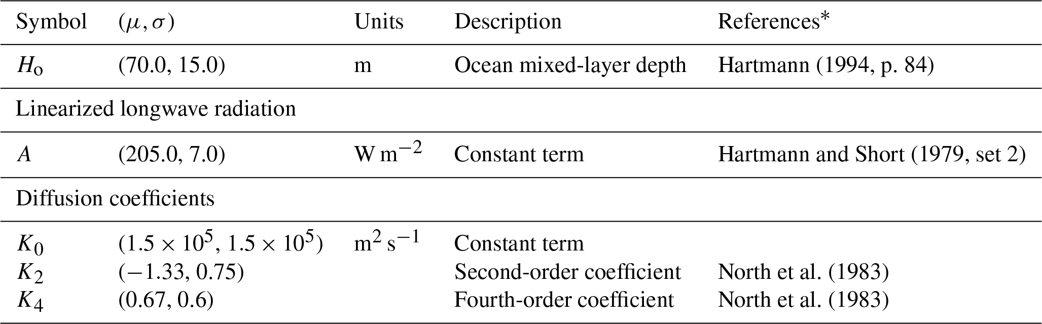
* References just for the mean values.
PL2012 evaluate several climate conditions and uncertain parameter scenarios, including present-day and Last Glacial Maximum (LGM) climate states. Then, with the model constrained by the present-day and LGM parameter estimates, they conduct climate projections under several CO2 forcing scenarios. We revisit their PD1 scenario: a present-day test with five (scalar) parameters, summarized in Table 1, as control variables. Here we summarize the model in relation to these parameters, and the reader is referred to PL2012 for a thorough description of all model parameters and related equations. The ocean mixed-layer depth, Ho, controls the effective heat capacity of the atmosphere–ocean system. A is a constant term in the calculation of the outgoing longwave radiation , which also depends linearly on the surface temperature and the logarithm of the ratio of the actual value of the atmospheric CO2 concentration to a reference value (Eq. 6 in PL2012). Meridional heat transport is treated as a diffusive process driven by latitudinal temperature gradients, whereby the horizontal heat transport depends linearly on a thermal diffusion coefficient Kao(x) given by , where K0, K2, and K4 are the remaining three parameters included in the control vector (Table 1), and x=sinΦ, where Φ is latitude.
3.2 Observations and cost function
As observations, we took surface air temperature (SAT) derived from the NCEP/NCAR reanalysis data (Kalnay et al., 1996). From the reanalysis data we first calculated global zonal means of SAT. Then, we obtained SAT means for present-day climate at each grid cell (i.e. latitude) for winter (January, February, and March; JFM) and summer (July, August, and September; JAS) in the Northern Hemisphere. These zonal averages of SAT, Ts, were the target for the analysis. The mean of the last 10 years, out of 100 years of model integration, was taken as the model equivalent of the observations. That is, each grid cell in the 1-D model has one observation and model equivalent for winter (JFM) and similarly for summer (JAS) in the cost function, defined by
where W is a diagonal matrix, whose diagonal is a vector of weights w∈ℝp given to the observations. This cost function can be written as . The observational target and control variables are identical to those in PL2012, but they did not include a background term 𝒥b in the cost function. Like PL2012, we assumed that observation errors are uncorrelated (R is diagonal), with all observations having a standard deviation C. The explicit division of the norm for 𝒥o in terms of R−1 and w facilitates the comparison of scenarios as a function of increasing observational weight.
3.3 Experimental set-up
Like PL2012, we set the grid resolution to 10∘. We assumed a diagonal , with standard deviations given in Table 1, which we considered as reasonable. Other than the parametric uncertainty we considered a perfect-model assumption, which is overly optimistic in this specific case as, in addition to the 1-D Earth climate representation, there are strongly simplified physics in the energy balance model. While PL2012 also assume this perfect-model framework, they point to a number of specific structural model errors. Thus, the control variables will attempt to compensate for the unaccounted error in either of the evaluated estimation approaches.
For the PD1 tests, we made the observation weights w proportional to the area of the zonal band (i.e. decreasing toward the poles) with , and we compared the FDS-MKS, the FDS-IKS, the ETKF (m=60 members), and 4D-Var. We evaluated a two-step and a three-step FDS-MKS (a one-step FDS-MKS equals an FDS-EKS or a first iteration of the FDS-IKS). To evaluate the resilience of the FDS schemes to high perturbations, we conducted three tests with different perturbation sizes for each FDS scheme. In each one, the perturbation applied to each of the control variables was proportional to its background standard deviation by a factor SDfac. This perturbation factor was . The evaluation of the cost function for the ETKF (as a smoother) was conducted with a single forward integration of the mean of the posterior control variables. In the 4D-Var minimization, like PL2012, we used a variable-memory quasi-Newton algorithm as implemented in M1QN3 by Gilbert and Lemaréchal (1989), and to compute the gradient we used a discrete adjoint approach with the tangent and adjoint codes generated automatically by the Transformation of Algorithms in Fortran (Giering and Kaminski, 1998; Giering et al., 2005). The number of simulations can be higher than the number of iterations as the minimizer M1QN3 takes a step size determined by a line search that sometimes reduces the initial unit step size (Gilbert and Lemaréchal, 1989). For 4D-Var, as a stopping criterion we required a relative precision on the norm of the gradient of the cost function of 10−4. For the assimilation in the ETKF and FDS tests we used rDAF (García-Pintado, 2018a) and rdafEbm1D (García-Pintado, 2018b), both working within the R environment (R Core Team, 2018).
We conducted a number of additional tests to compare the convergence of the FDS-IKS versus the FDS-MKS as higher weight is given to the observations. These were named PD2 and PD3, corresponding to and , respectively. As these weights increase, the effect of the regularization by 𝒥b decreases, and one can expect the convergence of the Gauss–Newton scheme (the FDS-IKS) to be more difficult. A few of these additional tests evaluate how and/or if the convergence of the FDS-IKS can be improved (mostly in a low-regularization situation) by increasing the number of perturbations per parameter (that is, the ensemble size). The results of these additional tests are briefly described here and expanded in Appendix A.
3.4 Results
Here we provide a succinct summary of the estimation process. Broader explanation of the model climatology in relation to the control variables is given in PL2012. The background sensitivity of the 10-year mean surface temperature Ts to the control variables is shown in Fig. 1 in which, to ease comparison, the sensitivity matrix G is scaled by multiplying each of its columns by the assumed background standard deviation of the corresponding parameter. Figure 1a shows mean ensemble sensitivities estimated from the background ensemble for the ETKF, and Fig. 1b shows local finite-difference sensitivities (FDSs) estimated with perturbations using SDfac=0.001. Note that these background FDSs are identical for both the FDS-IKS and the FDS-MKS in all scenarios (PD1, PD2, and PD3) for the same SDfac. Each plot has its own scale to avoid flattened lines in the ensemble sensitivity plot. For the three control variables composing the thermal diffusion coefficient Kao, FDSs are more than twice as high as the corresponding mean ensemble sensitivities. However, the sensitivities to the ocean mixed-layer depth, Ho, and to the constant term A in the longwave radiation are quantitatively similar in both cases. In both, A is negatively correlated (as expected) with Ts at all latitudes but with a relatively low sensitivity, while the rest of the control variables show a rather neutral, but negative, sensitivity in the tropical belt and a positive sensitivity increasing toward the poles (nearly symmetrical off the Equator), with weaker scaled sensitivities for the ocean mixed-layer depth Ho. In both cases, additional plots (not shown) depict summer sensitivities similar to the corresponding winter ones. Also, FDSs with SDfac=0.01 (winter and summer) are very similar to those shown in Fig. 1b. FDSs with SDfac=0.1 are also very close to those in Fig. 1b, but slightly lower for the Kao components, toward those in Fig. 1a.
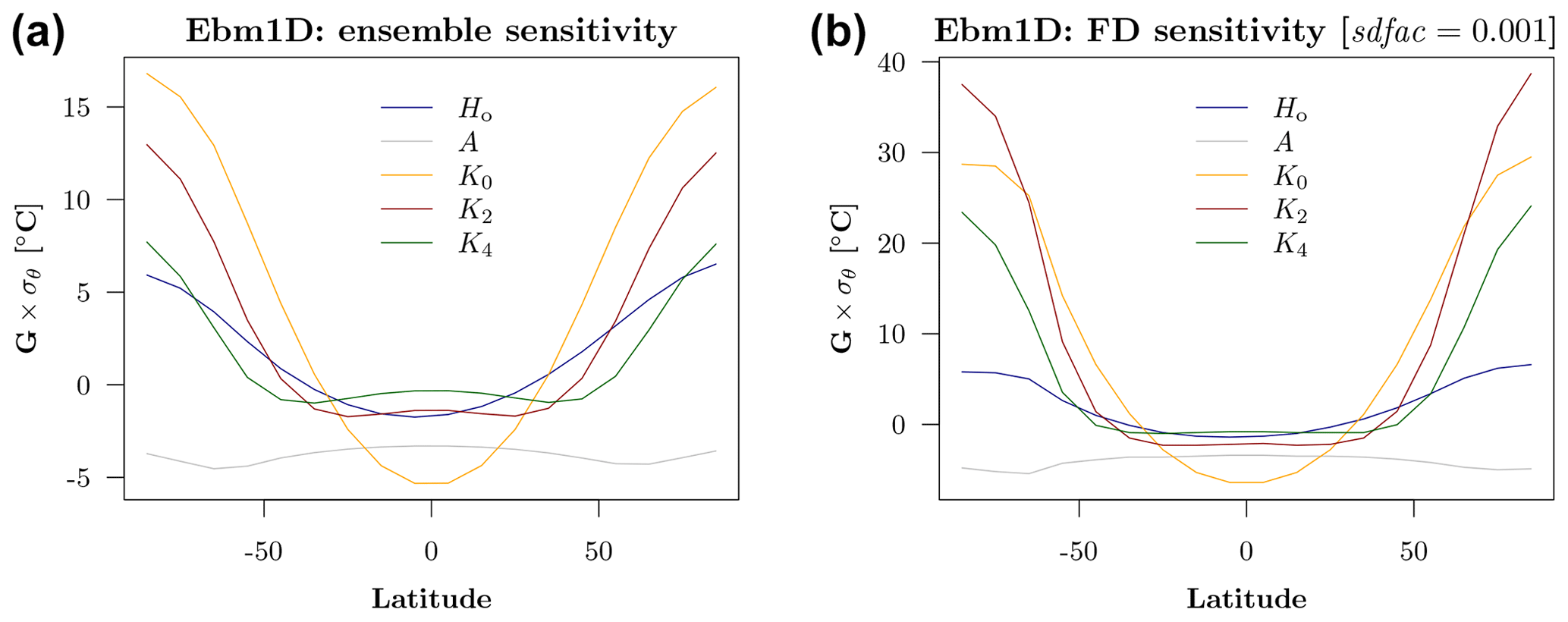
Figure 1Ebm1D experiment. Background sensitivity of winter surface air temperature to the control variables estimated as (a) ensemble sensitivity (for the ETKF) and (b) finite-difference sensitivity (for the FDS-IKS and the FDS-MKS) with SDfac=0.001. Sensitivities are scaled by the standard deviation of the control variables, and each line refers to a column in G. Each plot uses its own scale to ease visualization.
For the PD1 scenario, Fig. 2 summarizes the convergence, including the FDS-IKS, the two-step and three-step FDS-MKS, and 4D-Var; Table 2 compares the posterior control variables and the corresponding cost function values for all the evaluated schemes. For comparison, the convergence in Fig. 2 is scaled as a function of the number of simulations, which, for five control variables, is six simulations per iteration in the forward FDS schemes. Convergence details are given in Appendix A. For the PD1 scenario, 4D-Var took 141 simulations and 111 iterations to converge to the minimum with the convergence criterion indicated in Sect. 3.3. A relatively improved convergence by including the regularization term 𝒥b can be seen by comparison with PL2012, whose cost function only considered the 𝒥o term and took 236 simulations and 190 iterations to converge (Table 3 in PL2012). In any case, Fig. 2 shows that the 4D-Var convergence became apparently similar to that of the FDS-IKS tests from simulation 40 onwards. In Fig. 2, the three convergence series for the FDS-IKS with the three different perturbation parameters () are represented with the same symbol. Starting with the same background cost function value 𝒥, the two series with show identical results, while the series with SDfac=0.1 is the one that has a higher cost after the first iteration but still reunites with the other two series after the second iteration. However, the variations in SDfac had a very minor effect on the FDS-MKS schemes. For the FDS-MKS schemes, we focus now on the end of their corresponding iterations. The two-step FDS-MKS, for all SDfac values, gives final 𝒥 values that are close to but slightly higher than those of the FDS-IKS at the same number of iterations. The same happens with the three-step FDS-MKS with respect to the third iteration of the FDS-IKS. For 4D-Var, the convergence goes slightly faster than for the FDS-IKS at simulation number six (first iteration of FDS-IKS), but then it goes slower than for the FDS-IKS after that.
Table 2Ebm1D PD1 tests. Parameter estimation and cost function values*.
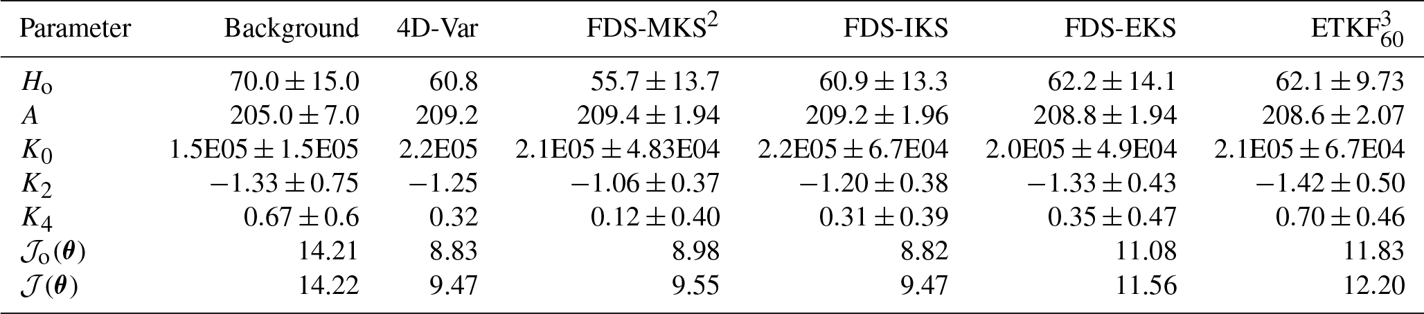
* FDS schemes with SDfac=0.001. Values are identical for SDfac=0.01 and slightly different with a minor increase in cost function values for SDfac=0.1 (see Appendix A). 2 Three-step FDS-MKS. Details of cost function convergence for the two-step FDS-MKS shown in Appendix A. 3 ETKF subindex indicates the ensemble size. Cost function obtained by reintegration of the model with the mean updated parameters.
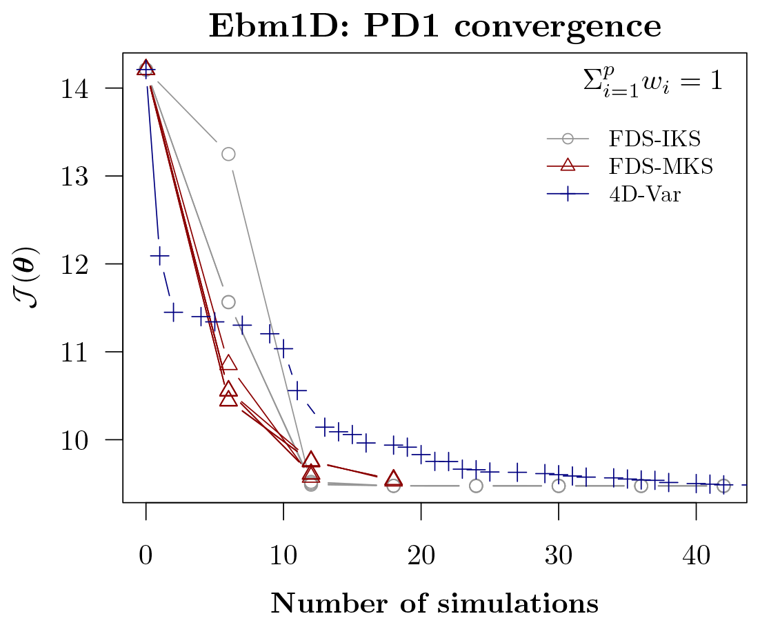
Figure 2Ebm1D experiment. Convergence as a function of the number of simulations for the scenario PD1 (). Each iteration of the evaluated finite-difference schemes requires six simulations (background plus number of perturbations, with one perturbation per parameter). Two-step and three-step FDS-MKS are included. Each FDS scheme includes the convergence for the three perturbation tests (details in text).
Table 2 for the PD1 scenario shows that the posterior values of the control variables, as well as the corresponding cost function values, are nearly identical for 4D-Var and the FDS-IKS (values shown for SDfac=0.001 perturbations, but also similar for the higher SDfac values). The three-step FDS-MKS also (shown for SDfac=0.001) converges to relatively similar control variables. In this case, the FDS-EKS (first iteration of FDS-IKS) also obtained lower cost function values than the ETKF. Although both obtained similar values for Ho, A, and K0, in the ETKF case, the values of K2 and K4 (with a clear non-linear relation with the surface air temperature) diverged from the minimum obtained by 4D-Var and the FDS-IKS. This is related to the background departure from the minimum and the mean sensitivities used by the ETKF. In general, one would not expect an FDS-EKS to perform better than an ETKF with denser sampling (bigger ensemble) as in this case. Table 2 also indicates the posterior standard deviations for the Kalman-based schemes. Non-diagonal values of are not shown. There are no high differences among the various posterior standard deviations for the Kalman-based schemes, with some values being higher in one scheme and others higher in a different scheme. In summary, the linear approaches (ETKF and FDS-EKS) obtained some reduction in the cost function values with respect to the background, but the rest of the schemes obtained substantially lower cost function values, with the FDS-IKS and 4D-Var converging to the same minimum and getting the lowest 𝒥 values. It is possible that an alternative minimization for the strong-constraint 4D-Var would have converged faster. In any case, the FDS-IKS has been shown to have a fast convergence in this experiment. Interestingly, Fig. 2 shows that the first fraction of all FDS-MKS schemes had a substantially lower cost value than either 4D-Var or any of the FDS-IKS tests. This, along with the resilience of the FDS-MKS to relatively high perturbations, supports the strategy of using a combination of the FDS-MKS in early iterations of a Newton-like scheme such as the FDS-IKS, akin to Wu et al. (1999) or Gao and Reynolds (2006). Alternatively, one can conduct a line search along the direction given by the FDS-IKS increments at each iteration. Further details for this experiment are in Appendix A, focusing on the convergence of FDS-IKS versus FDS-MKS as the observational weight increases.
4.1 Experimental set-up
Experiment 2 is a synthetic test with the Community Earth System Model (CESM1.2), a deterministic ESM. The CESM component set used here comprises the Community Atmosphere Model version 4 (CAM4), the Parallel Ocean Program version 2 (POP2), the Community Land Model (CLM4.0), the Community Ice CodE (CICE 4) as a sea ice component, the River Transport Model (RTM), and the CESM flux coupler CPL7. The coupler computes interfacial fluxes between the various component models (based on state variables) and distributes these fluxes to all component models while ensuring the conservation of fluxed quantities. Land ice is set as a boundary condition, and the wave component is not active. The configuration uses pre-industrial forcings and it is a standard component set named B1850CN in the CESM1.2 list of compsets. We use a horizontal resolution regular finite-volume (FV) grid for the atmospheric and land components, an FV grid with a displaced pole centred at Greenland (version 7) for the ocean and sea ice components, and a 0.5∘ FV grid for the river run-off component (this is also a standard set of component grids with short name f45_g37 in CESM1.2). For comparison, this is a coarser resolution than that of the recent CESM Last Millennium Ensemble (Otto-Bliesner et al., 2016).
Here we focus on the analysis for a single DAW and equilibrium forcing and, as adequate, introduce some comments regarding practical implementations for real cases, including the case of transient forcings. The identical twin assimilation experiment is designed to approach a case of past climate reconstruction with sparse observations, as usual in pre-instrumental climate analysis. Specifically, we use the features of available observations of near sea surface temperature for the Last Glacial Maximum (LGM) from the MARGO database (MARGO Project Members, 2009). The LGM has received great attention in the paleoclimate community for its relevance to understand climate feedbacks and future climate projections; specifically, the MARGO database has been profusely used for qualitative and quantitative model–data comparisons (e.g. Kageyama et al., 2006; Hargreaves et al., 2011; Waelbroeck et al., 2014) as well as in dynamical reconstruction, with the ocean model MITgcm and 4D-Var, of the upper-ocean conditions in the LGM Atlantic (Dail and Wunsch, 2014) and the global ocean (Kurahashi-Nakamura et al., 2017). For the purpose of this study, it is not so important that the actual climate of the model matches that of the LGM but that the case study is realistic from the estimation point of view. Thus, we make use of the MARGO database characteristics (location, seasonality, and uncertainty), but conduct a synthetic experiment for pre-industrial climate conditions. To do so, before starting the experiment we spun up CESM for 1200 years starting from Levitus climatology with standard pre-industrial conditions to reach an equilibrium state. Then, we used the restart files from the end of the spin-up time to create a 60-year control simulation (as synthetic truth), in which in addition to the pre-industrial forcings and boundary conditions, we added a flux term to the ocean, as detailed below.
To create the background ensemble we perturbed a number of parameters for the (deterministic) physics in both the ocean and the atmosphere components, as well as input greenhouse gases and an additional influx of water into the North Atlantic Ocean. As indicated in the Introduction, the selected control variables have the responsibility of creating all the background uncertainty in a perfect-model scenario, and through the assimilation they will try to compensate for any unaccounted model error elsewhere. In a step-by-step approach, here all perturbed model parameters and forcings were included as control variables in the assimilation. An obvious (still synthetic) and very useful extension would be to perturb a wider set of model parameters and/or forcings and boundary conditions (e.g. various ice sheet configurations or alternative freshwater influx) and explicitly evaluate the compensation effect and climate reconstruction results by using subsets of the perturbed inputs as control vectors. Here, the selected parameters for model physics and radiative constituents are relevant to the global energy budget of the Earth system, but not necessarily the most sensitive model inputs for multi-decadal and longer scales. In real cases, the selection of control variables (if the control vector is to be kept low-dimensional) should be done carefully and generally based on previous global sensitivity analyses.
We included an influx of water into the North Atlantic from melting in the Greenland ice sheet (GIS) to the true run and as a control variable. This flux was homogeneously distributed along the coast of Greenland and at the ocean surface, and it is appealing to explore as a control variable because the Atlantic meridional overturning circulation (AMOC) plays a critical role in maintaining the global ocean heat and freshwater balance. It is commonly acknowledged that North Atlantic deep water (NADW) formation is key in sustaining the AMOC (Delworth et al., 1997), while in turn freshwater flux in the North Atlantic, along with surface wind forcing, ocean tides, and convection, provides the energy for NADW formation (Gregory and Tailleux, 2011). Adding this freshwater flux (or freshwater hosing) makes the identification of the model parameters more complicated, but it is realistic to expect that current paleoclimate melting estimates can hold some bias and it is useful to know how the evaluated schemes deal with this possibility. In real cases, flux terms have been used in paleoclimate modelling to account for model errors. So, they relax the perfect-model assumption in a parametric way. Here, the estimated flux term attempts to correct the mean state towards the observations along with the model parameters. As far as the authors know, this is the first experiment with a comprehensive ESM which attempts (even in a synthetic way) a joint flux and model parameter estimation for climate field reconstruction, as these are more commonly seen as competing strategies.
We initiated the background with biased control variables with respect to the truth and a zero-mean Greenland ice sheet freshwater flux. We used reasonable uncertainties in the control variables derived from previous publications. Separate analyses (weakly coupled assimilation) for different model components (atmosphere, ocean, land) may be inconsistent. In our set-up, all observations are allowed to directly impact model parameters from any component in the Earth system model. This is known as strongly coupled data assimilation. Both truth and background simulations were branched from the same initial conditions, which allowed us to use relatively short integration times (60 years) in the experiment. In a real case with steady-state forcings (e.g. estimation of real LGM climate state by assimilating the MARGO database), the model should be integrated even longer towards quasi-equilibrium to ensure that errors in the initial conditions will not affect the analysis (or they should be accounted for). Also, each model equivalent of the observations has to be mapped into the corresponding spatio-temporal domain of each paleoclimate proxy observation. Similar to the previous experiment, for the FDS schemes, we set the perturbations for each control variable as equal to their standard deviation multiplied by a perturbation factor SDfac. For computational reasons we only tested .
The cost function was as in Eq. (17), in which the set of control variables used for the experiment is summarized in Table 3. Sect. 4.2 and 4.3 give brief information on the atmospheric and ocean components of CESM as used in this experiment. For the rest of the model components we used default configurations for the indicated CESM compset. Given that adjoint codes are not available for CESM, here we alternatively tested an ETKF (with m=60 ensemble members) including Gaussian anamorphosis (ETKF-GA) as a possible non-linear approach, which has a negligible extra cost over a standard ETKF. We also evaluated the three-step FDS-MKS, the FDS-IKS (with three as the maximum number of iterations), and the ETKF, also with m=60. For all the assimilation analyses we used rDAF (García-Pintado, 2018a), and rdafCESM (García-Pintado, 2018c).
4.2 CAM
We used the Community Atmosphere Model version 4 (CAM4) as an atmospheric global circulation model (AGCM) component. A comprehensive description of CAM4 can be found in Neale and Coauthors (2011). Precipitation and the associated latent heat release drive the Earth's hydrological cycle and atmospheric circulations, and many model processes in AGCMs, including deep and shallow convection and stratiform cloud microphysics and macrophysics, are responsible for the partitioning of precipitation through competition for moisture and cooperation for precipitation generation (Yang et al., 2013). Cumulus convection is a key process for producing precipitation; it is also key for redistributing atmospheric heat and moisture (Arakawa, 2004) and, consequently, the global radiative budget (Yang et al., 2013). Since AGCMs are unable to resolve the scales of convective processes, various convection parameterization schemes (CPSs) have been developed based on different types of assumptions. The CPS usually includes multiple tunable parameters, which are related to the sub-scale internal physics and are thought to have wide ranges of possible values (Yang et al., 2012). Also, the dependence of CPS parameters on model grid size and climate regime is an important issue for weather and climate simulations (Arakawa et al., 2011). In addition, AGCMs include parameterization of macrophysics, microphysics, and subgrid vertical velocity and cloud variability to simulate the subgrid stratiform precipitation.
Here we used CAM4 with the Zhang and McFarlane (1995) deep convection scheme and the Hack (1994) shallow convection scheme. For representation of stratiform microphysics we used the scheme by Rasch and Kristjánsson (1998), which is a single-moment scheme that predicts the mixing ratios of cloud droplets and ice. Regarding cloud emissivity, clouds in CAM4 are grey bodies with emissivities that depend on cloud phase, condensed water path, and the effective radius of ice particles. By default, the CAM4 physics package uses prescribed gases except for water vapour. In CAM4, the principal greenhouse gases whose longwave radiative effect is included are H2O, CO2, O3, CH4, N2O, CFC11, and CFC12. CO2 is assumed to be well mixed. As the use of prescribed species distributions is computationally less expensive than prognostic schemes, for long-term paleoclimate analysis we would generally favour the use of prescribed greenhouse gases, for example as given by the recently published 156 kyr history of atmospheric greenhouse gases by Köhler et al. (2017). Still, we would acknowledge that these emerging datasets have an associated uncertainty and that it is generally appropriate to include the most influential ones as control variables in the climate analysis so their errors can be estimated as part of the assimilation.
In this study, as perturbed parameters and control variables we selected parameters related to the ZM deep convection scheme and the relative humidity thresholds for low and high stable cloud formation. Also, within the radiative constituents, we included invariant surface values of CO2 and CH4 as control variables. Table 3 shows the control variables in both CAM and POP2, and Table 5 shows the true run values in column xt.
Table 3CESM definition of control variables.
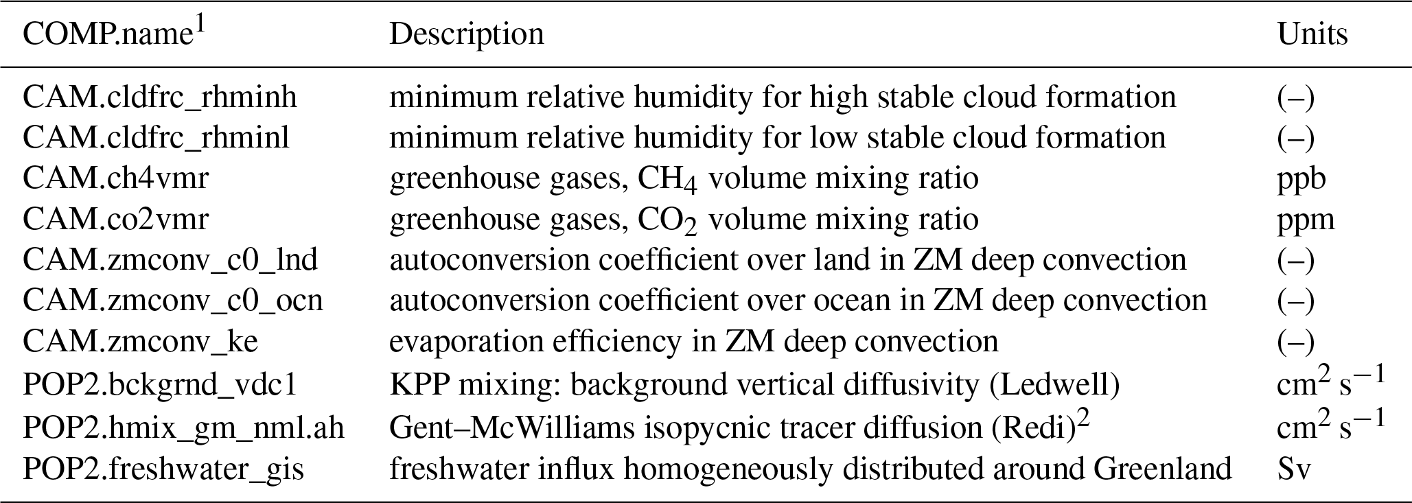
1 COMP.name: CESM component and parameter name. 2 We constrained POP2.hmix_gm_nml.ah_bolus to equal POP2.ah.hmix_gm_nml.ah in the background and updates.
This experiment is based on equilibrium simulations. Regarding real cases in transient conditions, θ could e.g. include a constant error term (i.e. a bias) for a transient greenhouse gas dataset as a prescribed radiative constituent in the atmospheric model (Köhler et al., 2017). The estimated bias would be updated for successive DAWs. One could think of more complicated autocorrelated error models for the greenhouse gas dataset (García-Pintado et al., 2013), but it seems highly unlikely to us that available proxy datasets for low-frequency climate variability can constrain errors further than simple biases in GHG forcing. We did not evaluate any parameter in relation to indirect effects of aerosol to cloud nucleation and autoconversion, despite the overall effect of aerosol to cloud albedo, cloud lifetime, and climate, so this remains largely uncertain (Chuang et al., 2012).
4.3 POP2
As an ocean component, we used POP2 (Smith et al., 2010). Subgrid-scale mixing parameterization includes horizontal diffusion and viscosity and vertical mixing. For horizontal diffusion we chose an anisotropic mixing of momentum and the Gent and McWilliams (1990) parameterization, which forces the mixing of tracers to take place along isopycnic surfaces with activated submesoscale mixing. The main drawback in the Gent and McWilliams (1990) scheme is that it nearly doubles the running time with respect to other simpler schemes. For vertical mixing, we chose the K-profile parameterization (KPP) of Large et al. (1994). In KPP mixing, the interior mixing coefficients (viscosity and diffusivity) are computed at all model interfaces on the grid as the sum of individual coefficients corresponding to a number of different physical processes. The first coefficients are denoted as background diffusivity κω and background viscosity υω (not to be confused with the “background” in assimilation terminology), which represents diapycnal mixing due to internal waves and other mechanisms in the mostly adiabatic ocean. Other coefficient are associated with shear instability mixing, convective instability, and diffusive convective instability. The background viscosity is allowed to vary with depth, but here we assumed a depth-constant vertical viscosity κω= bckgrnd_vdc1, where bckgrnd_vdc1 is a model input parameter. The model then computes υω=Prκω, where Pr is the dimensionless Prandtl number (set to Pr =10 in the model).
As control variables in POP2 we chose the Gent–McWilliams isopycnic tracer diffusion parameter and the (constant with depth) KPP background viscosity, both with default values for the truth. A third control variable in POP2 was the total freshwater influx from the Greenland ice sheet, which we distributed homogeneously along the coast of Greenland and only at the ocean surface.
4.4 Observations
The observational dataset is composed of point samples of climate averages for the last 20 years out of a total 60 years of integration time in a true simulation. The synthetic observations were located at the horizontal locations and 10 m of depth of the MARGO database, and the sampling characteristics reproduce those of MARGO. The MARGO database is a synthesis of six different proxies and is considered to represent the combined expertise of at least a sizeable fraction of the LGM paleocommunity. The observational uncertainty was taken from the MARGO database as input to the assimilation, but we did not add any error to the synthetic observations. MARGO provides observations (or reconstructions) of near sea surface temperature (SST) for the Last Glacial Maximum (LGM). The proxy types on which the SST estimates are based are (a) microfossil based (planktonic foraminifera, diatom, dinoflagellate cyst, and radiolarian abundances) and (b) geochemical paleothermometers (alkenone unsaturation ratios () and planktonic foraminifera Mg ∕ Ca). Details on the database are given in MARGO Project Members (2009).
In summary, MARGO provides seasonal means for Northern Hemisphere winter (January, February, and March; JFM) and summer (July, August, and September; JAS), as well as annual means. However, the data availability for each of the three temporal means (winter, summer, and annual) is different for each proxy type. Specifically, diatoms are just available for Southern Hemisphere summer; dinoflagellates, foraminifera, and Mg ∕ Ca are available for the three temporal means; and values are only available as annual means. The observation errors are assumed uncorrelated, but each individual record in MARGO contains a specific uncertainty. Mapped into the SST space, the range of standard deviations in MARGO is within 0.79 and 4.87 ∘C, with relatively homogeneous uncertainty ranges among proxy types. Figure 3 shows the type and location of the proxy data. In addition to the locations and uncertainty, we emulated the temporal mean availability of the observations, with all temporal means calculated over the last 20 years of the integration time in the true simulation. Thus, the synthetic observations in the experiment, as well as those in MARGO, impose a less restrictive constraint not only in areas in which observations are more sparse, but also in those locations for which just one season or just annual means are available.
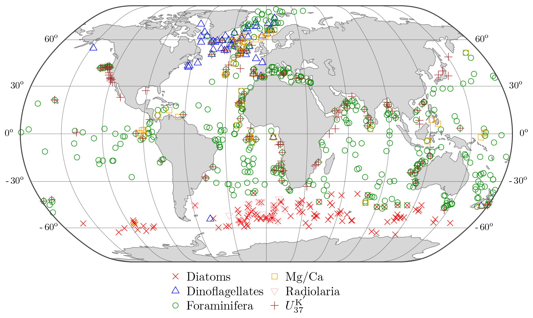
4.5 Results
4.5.1 Non-linearity and Gaussian anamorphosis transformations
The need for non-linear estimation is justified based on the assumed non-linear relationship between the control variables and the observation space. In this experiment, non-linearity is imposed by the Earth system model, which directly generates SST as the observed variable. In a more general case of past climate analysis, the forward operator (proxy system model) can impose further non-linearity when the observed variables are direct proxy records (e.g. foraminiferal counts, tree-ring widths, speleothems, etc.). In addition to model and forward operator non-linearity, non-Gaussianity in the control variables also renders (En)KF non-optimal. Here we conducted a test with ETKF including the Gaussian anamorphosis (GA) transformation (ETKF-GA). The test transforms the control variables, whose background deviations from Gaussianity here derive from imposed bounds, and the SST in both the model equivalent of the observations and the observations themselves with the strategy explained in Sect. 2.6. In this section, we show an example of non-Gaussianity and non-linearity in this experiment, which are the motivation for the iterative FDS schemes evaluated in this paper as well as for testing the Gaussian anamorphosis. Specific estimation results are given in Sect. 4.5. Note that no transformation has been applied to the FDS schemes.
In the ETKF-GA test, we conducted the marginal Gaussian anamorphosis for all the variables in the control vector. Table 4 shows the p values of the Shapiro–Wilk normality test (Shapiro and Wilk, 1965) conducted on the original (raw) control vector and the anamorphosed ones (ana). The second column shows that Gaussianity is improved in all cases, with most of them even reaching a p value =1. We note that despite the fact that the GA was applied to all the control vectors, the raw samples of the background control variables also had a p value > 0.05 in all cases. For the SST observations, we evaluated the marginal normality of the raw SST with the Shapiro–Wilk test. Then, we only applied the GA transformations at locations with the background SST deviating significantly from Gaussianity.
Table 4CESM experiment. P values of Shapiro–Wilk normality test for the ensemble of original control variables (Raw) and transformed by Gaussian anamorphosis (Ana).
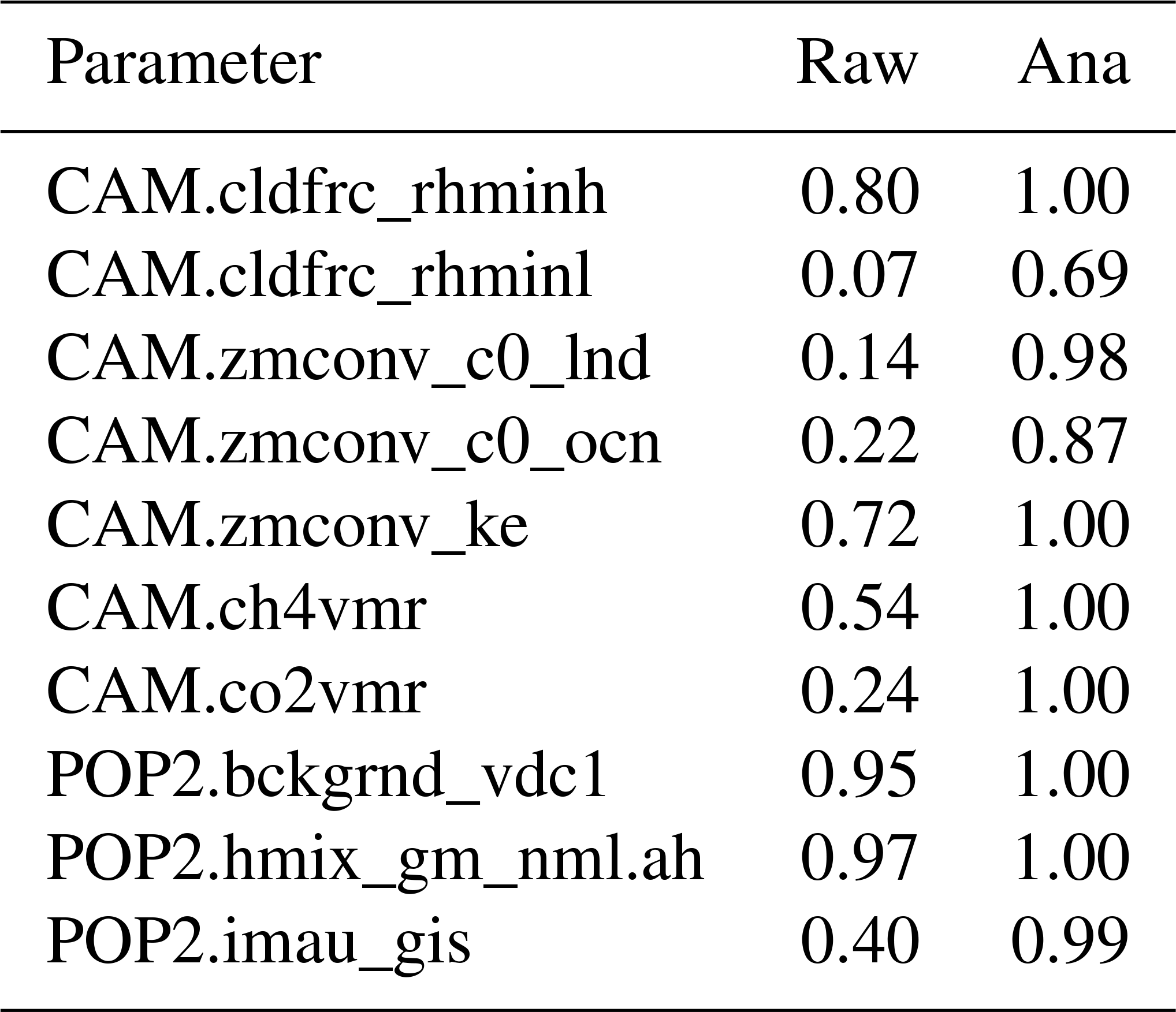
The minimum relative humidity for high stable cloud formation (CAM.cldfrc_rhminl parameter), given its background uncertainty, was shown to have a strong effect on SST in the experiment. In most locations of the global ocean the marginal background SST had a non-Gaussian but still unimodal probability density function. Especially complicated was the North Atlantic, with strongly bimodal background distributions in some locations. One of these cases is depicted in Fig. 4. As shown in Table 4, the CAM.cldfrc_rhminl parameter had a sharp increase in its background Gaussianity in the anamorphosed variable, and Fig. 4a describes the transformation of SST in a location in the North Atlantic Ocean. Specifically, this is the observation with the highest negative innovation in the experiment, and it seems to represents the most complicated case in the test. Apart from the high (negative) innovation, the raw observation falls well in the tail of the transformation, so its forward and backward transformations are rather sensitive to the dealing of the tails in the anamorphosis function, as mentioned in Sect. 2.6 and Simon and Bertino (2009, 2012). In addition, there is the effect of bimodality in SST in this case. As a result, despite both marginal transformations (control variable and SST) having a clear increase in their marginal Gaussianity, their joint distribution is not bivariate Gaussian, as seen in Fig. 4b. This generic possibility is also very well described by Amezcua and Leeuwen (2014). Appendix B shows an example of the more general case, in which the Gaussian anamorphosis does not show specific issues.
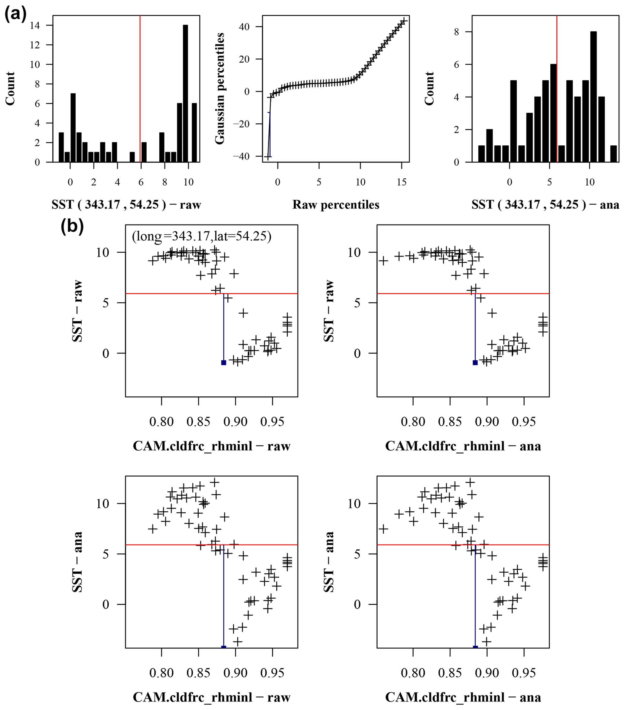
Figure 4CESM experiment. Example of Gaussian anamorphosis transformation in a control variable (minimum relative humidity for high stable cloud formation) and the sea surface temperature (SST) for both the model equivalent of the observations and the observation (transformation details in text) at a location (343.17∘ E, 54.25∘ N; see Fig. 5) in the North Atlantic, where an apparent switch in SST takes place. (a) The anamorphosis for the SST at the location; the left panel shows the histogram of the original (raw) variable, the middle panel shows the empirical piecewise linear transformation which maps the raw variable percentiles into those of a normal variable with the two first moments (mean and standard deviation) preserved as those in the raw variable, and the right panel shows the histogram of the anamorphosed variable. (b) Scatterplots between the two variables in (a) for the original variables: cases in which only one is transformed and the case with both variables transformed. Vertical red lines in (a) and horizontal lines in (b) indicate the mean of the model background SST. Blue squares indicate observations, vertically placed and connected with the mean of the control variable.
4.5.2 Sensitivities and minimization
Table 5 shows the values of the control variables for the true simulation, xt, the background (or prior), xb, and the analysis (or posterior) estimates, xa, for the evaluated schemes, as well as the value of the cost function 𝒥 for the background and each estimation. The observational term in the cost function, 𝒥o, is also shown to give an indication of the relative contribution from each cost function term. 𝒥o is calculated by reintegration of the updated (or posterior) control vector in the FDS schemes and reintegration of the mean of the updated control vector ensemble for the ETKF and the ETKF-GA. An initial experiment with the perturbation factor SDfac=0.001 showed extremely high sensitivities, and the corresponding FDS-EKS (or first step of the FDS-IKS) had a very small increment in the control vector variables. The scale of sensitivities for a perturbation factor SDfac=0.1 was more in agreement with the ensemble sensitivities of the ETKF background (and higher increments in a good direction), and we decided to apply this perturbation factor to both the FDS-MKS and FDS-IKS. Still, according to the previous experiment, these high perturbation factors should favour the (more regulated) FDS-MKS. All the following results refer to SDfac=0.1. Due to limits in the computational quota, we did not test alternative perturbation factors in this experiment. It is very likely that smaller perturbations (e.g. SDfac∼0.01) would have resulted in improved results for the FDS schemes, mostly for the FDS-IKS. Thus, in a way, the results here may be interpreted as relatively low performance bounds for the FDS schemes under the given experimental assumptions.
Table 5CESM control vector estimation1.
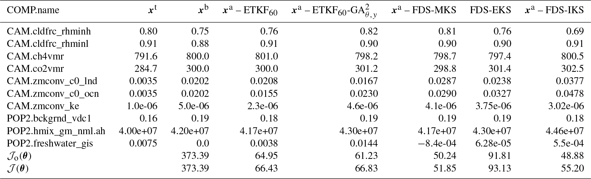
1 Units as described in Table 1. 2 ETKF subindex indicates the ensemble size. Cost function obtained by reintegration of the model with the mean updated parameters.
All schemes obtained a substantial reduction in the value of the cost function with respect to the background, which had a 𝒥(θb)=373.39. Within the evaluated schemes, the three-step FDS-MKS obtained the lowest cost function value with 𝒥(θa)=51.85. The cost for the FDS-IKS (stopped at the third iteration) was slightly higher (𝒥(θa)=55.20). However, the observational term 𝒥o(θa) was lower for the FDS-IKS. The m=60 member ETKF resulted in a higher cost value (𝒥(θa)=66.43) and the ETKF-GA in a very similar 𝒥(θa)=66.8. As expected, the FDS-EKS (or first iteration of the FDS-IKS) resulted in the highest cost value, with 𝒥(θa)=93.13, as it is linear (as the ETKF), and also the FDS-reduced exploration of the sensitivity is noisier than that of the ETKF with m=60 members. The cost function for the thee iterations of the FDS-IKS is shown in Table B1.
As seen, regarding the cost function, the Gaussian anamorphosis (as implemented here) did not improve the minimization with respect to the ETKF, although the transformation served to obtain a lower value for the observational term 𝒥o. Out of several transformation possibilities, Amezcua and Leeuwen (2014) concluded that using the CDF estimated from the ensemble model equivalent of the observations to also transform the observations (as done here given the considerations indicated in Sect. 2.6) was the worst option. In any case, we have also seen here a specific example that shows that even if marginal Gaussianity is improved in both transformed control variables and the model equivalent of the observations, the joint probability is not guaranteed to be bivariate Gaussian (Fig. 4). It is also interesting to note that the slope of the scatterplot examples shown in Fig. 4 is positive for the two separate branches of an apparent switch occurring in SST (with a sharp negative step in SST around CAM.clfrc_rhminl=0.88) at this location in the North Atlantic. Thus, the slope for a linear regression in this relation would have been clearly negative, as opposed to the slopes in the individual two branches. This switch in SST here seems to be associated with a displacement in the North Atlantic gyre and (possibly coupled) cloud development. This general negative slope in SST with respect to CAM.cldfrc_rhminl is clearly shown at the given location in the ensemble sensitivity plot in Fig. 6. The switch also indicates that the background values and perturbation sizes are key for FDS estimation and indicates why the corresponding SST plot for FDS in Fig. 6 differs substantially from the ensemble sensitivity at the given location (note that the sensitivity about the background is the same for both FDS schemes: the FDS-MKS and the FDS-IKS). Additional sensitivity plots (not shown) also indicate a positive mean ensemble sensitivity of both total cloud cover and large-scale precipitation with respect to the CAM.clfrc_rhminl at this location, while the sensitivity of the cloud cover to CAM.clfrc_rhminl becomes negative for latitudes lower than 50∘ N in the North Atlantic. A major point here is that the Gaussian anamorphosis cannot solve the strong non-linear relationship in this case. Also, the MARGO coverage is far denser in the North Atlantic than in the rest of the global ocean. Thus, the updates to global parameters in the control vector are strongly influenced by the sensitivities in the area. The MARGO coverage in the North Atlantic can be adequate regarding the analysis of the glacial climate at the LGM, and here it has been useful to show that the anamorphosis, as applied here, has not been able to solve the strong non-linearities found in the North Atlantic area. Still, in other conditions with available proxy time series, one could possibly apply alternative transformations for the observations based on their own statistics, and results could perhaps improve. Also, a further evaluation of the specific contribution from each observation to the increments could serve to design quality controls and improved ensemble approaches. By only looking at the posterior estimates in Table 5, it does not seem possible to derive any general conclusions about the benefit of the Gaussian anamorphosis in ensemble Kalman schemes for multi-decadal climate analysis from the view of this experiment, but further exploration is needed.
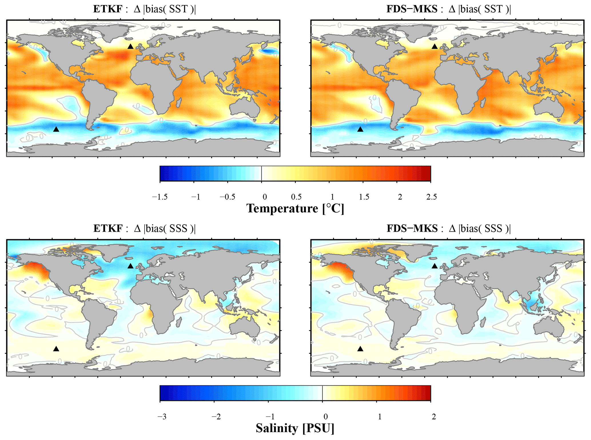
Figure 5CESM experiment. Absolute bias reduction for SST and SSS as a result of a new integration with the parameters estimated with the ETKF and the FDS-MKS. The statistics are the absolute bias between the background and the truth minus the absolute bias between the analysis and the truth. Thus, positive values are a net bias reduction. Isolines at value 0 shown in grey. The two triangles indicate the locations in the North Atlantic and South Pacific connected with Figs. 4 and B1.

Figure 6CESM experiment. Sensitivity of SST (∘C) and SSS (PSU) to the minimum relative humidity for low stable cloud formation (CAM.clrfrc_rhmin) estimated from the ETKF background ensemble and the first iteration of the FDS-MKS. Isolines at value 0 shown in grey.
The lower cost function values of the FDS schemes with respect to the ETKF (with and without GA) suggest a benefit in the more limited (and noisier) but iterated local sensitivity estimation. Also, the computational cost in the FDS tests was about half of the ETKF (and ETKG-GA). Regarding the estimation of specific control variables, all of the evaluated schemes had some variables for which the estimation, starting from the background, went in the wrong direction with respect to the true values. For example, the closest estimate to the true value of the relative humidity threshold for high stable cloud formation (cldfrc_rhminh) was given by the FDS-MKS, with a slight overshooting (0.81 versus 0.80 for the truth). It may have been that this slight overshooting has partially compensated for the effect of other control variables. Thus, the FDS-MKS estimates of the freshwater flux from the Greenland influx went in the wrong directions, as did the estimates for the autoconversion coefficients in the Zhang–McFarlane deep convection scheme. On the other hand, the FDS-IKS had a total increment in cldfrc_rhminh in the wrong direction, but had the Greenland influx total increment in the right direction. The ETKF did not show any overshooting, but had some control variable increments going in the wrong direction. For the ocean background vertical diffusivity, the only two schemes for which there was some, albeit minor, improvement in the estimate were the ETKF and the FDS-IKS. Still, the improvement is so slight in these cases that it could be a random effect.
The perturbations in the FDS may have been far from optimal for sensitivity estimation regarding their effect on the model SST at the locations (including depth) of the observations for the integration times. Table B2 shows the corresponding standard deviation for the background and posterior estimates in the ensemble and iterated FDS schemes. In general, the posterior variance of the control vector was higher for the ETKF and the ETKF-GA and a bit smaller in the FDS schemes, but also the relative reduction in variances with respect to the background was not systematically lower or higher for any specific scheme.
In sensitivity studies, the conditional sensitivity exploration of the FDS has also been termed one-at-a-time (OAT) sensitivity analysis. The difference between the local sensitivities of the FDS and the mean sensitivities of the ensemble for the ETKF may affect the estimation of the various parameters to different degrees. For comparison, with a prescribed SST, Covey et al. (2013) evaluated the sensitivity of the radiation balance at the top of the atmosphere in the model CAM to a large number of input parameters with both an OAT exploration and an alternative Morris one-at-a-time (MOAT) sampling (somehow closer to the mean ensemble sensitivities). They found with both methods that the highest sensitivity of the upward shortwave flux (solar energy reflected back to space by the atmosphere and surface) was with respect to cldfrc_rhminl, out of 21 evaluated CAM parameters. As cldfrc_rhminl is the threshold of the relative humidity value at which low-level water vapour starts to condense into cloud droplets, their result is consistent with the role of thick stratus clouds in reflecting sunlight.
This study does not attempt to give an in-depth analysis of the assimilation results for the corresponding climate field reconstructions. However, we summarize some results of the spatial patterns shown in the climate reconstructions and give examples of sensitivities as estimated by the FDS schemes and the ETKF. Figure 5 shows, in general, a similar absolute bias reduction for the FDS-MKS and the ETKF in magnitude and spatial patterns for both SST and SSS. For SST, the most problematic area is where most of the observations come from the diatom locations in the MARGO database. A reason for that seems to be that observations for diatom locations are just the 20-year means for winter in the Northern Hemisphere, which reduces the impact on the climate analysis with respect to other observation types. Still, in general the FDS-MKS has slightly fewer areas where the absolute bias in the SST could not be reduced. The negative effect of the assimilation regarding absolute bias reduction on SSS, which is shown for the ETKF for the North Atlantic, the Bering Strait, and in some areas of the Arctic Ocean, is also negligible in the FDS-MKS. While these unobserved areas (from the point of view of the MARGO database) remain largely unconstrained, the FDS-MKS seems generally more able to correct for the biases in areas with more observations and simultaneously does not have a negative effect in areas far from the observations.
As an example of estimated sensitivities in the ocean, Fig. 6 shows the sensitivity of the sea surface temperature (SST) and sea surface salinity (SSS) to cldfrc_rhminl in CAM as mean ensemble sensitivities and FDS about the background value. In the case of SST the general pattern of both sensitivities is quite similar, except for the much more negative sensitivity shown at the North Atlantic Ocean above 50∘ of latitude for the ETKF, as detailed above. The second loop of the FDS-MKS (not shown) shows a similar pattern to the first loop. However, the sensitivity in the third loop (not shown) approaches the sensitivity of the ETKF and also shows a similar negative sensitivity area, in extent and magnitude, in the North Atlantic. Something similar happens to the sensitivity estimates for the SSS, for which the FDS in the first and second loops of the FDS-MKS are reasonably similar to the mean from the ensemble background for the ETKF, with the major differences being in the Arctic Ocean, around the Bering Strait, and the North Atlantic. The third loop of the FDS-MKS (not shown) also shows the more homogeneous band of sensitivity between the coasts of Canada and Europe shown for the ETKF.
Vertical diffusion in the ocean determines ocean heat uptake and in turn the air–sea heat flux and atmospheric heat transport, but also sea surface temperature, evaporation, and atmospheric moisture transport. Regions more sensitive to ocean vertical diffusion would be coastal upwelling systems (e.g. Namibia), the equatorial oceans, and the Southern Ocean in the case of upwelling, but also the North Atlantic Ocean in the case of downwelling (deep water formation), which is key in sustaining the Atlantic meridional overturning circulation (AMOC) (Delworth et al., 1997). Thus, as a further example in the ocean, we also find it interesting to show a sensitivity example for deeper ocean layers considering the short integration time (60 years) of the experiment. For this integration time the deep ocean is far from reaching equilibrium, but the maximum value of the AMOC has reasonably converged in the perturbed members for the ETKF and in the FDS-MKS members for the three iterations. Figure 7 depicts the sensitivity of the AMOC to the background vertical diffusivity (κω; POP2 parameter bckgrnd_vdc1) for the ETKF and the three iterations of the FDS-MKS. It can be seen that the general pattern has some similarities in all cases, but also noticeable differences. The first iteration of the FDS-MKS (FDS-MKS.f01) is quite close to the mean estimate of the ETKF, except for the high-sensitivity area around 30∘ N and at 1.5 km deep, which is mostly missing in the FDS-MKS.f01. The pattern of sensitivity in the second iteration (FDS-MKS.f02) is similar to that in the first iteration but with much higher values. The third loop again has reduced sensitivities and keeps missing the deeper high-sensitivity area given by the mean sensitivity of the background ensemble for the ETKF. This warrants further study to analyse with more detail why, despite sampling different regions of the parameter space, the conditional parameter sampling of the FDS-MKS does not show in any case the deeper high-value area estimated by the mean sensitivity.
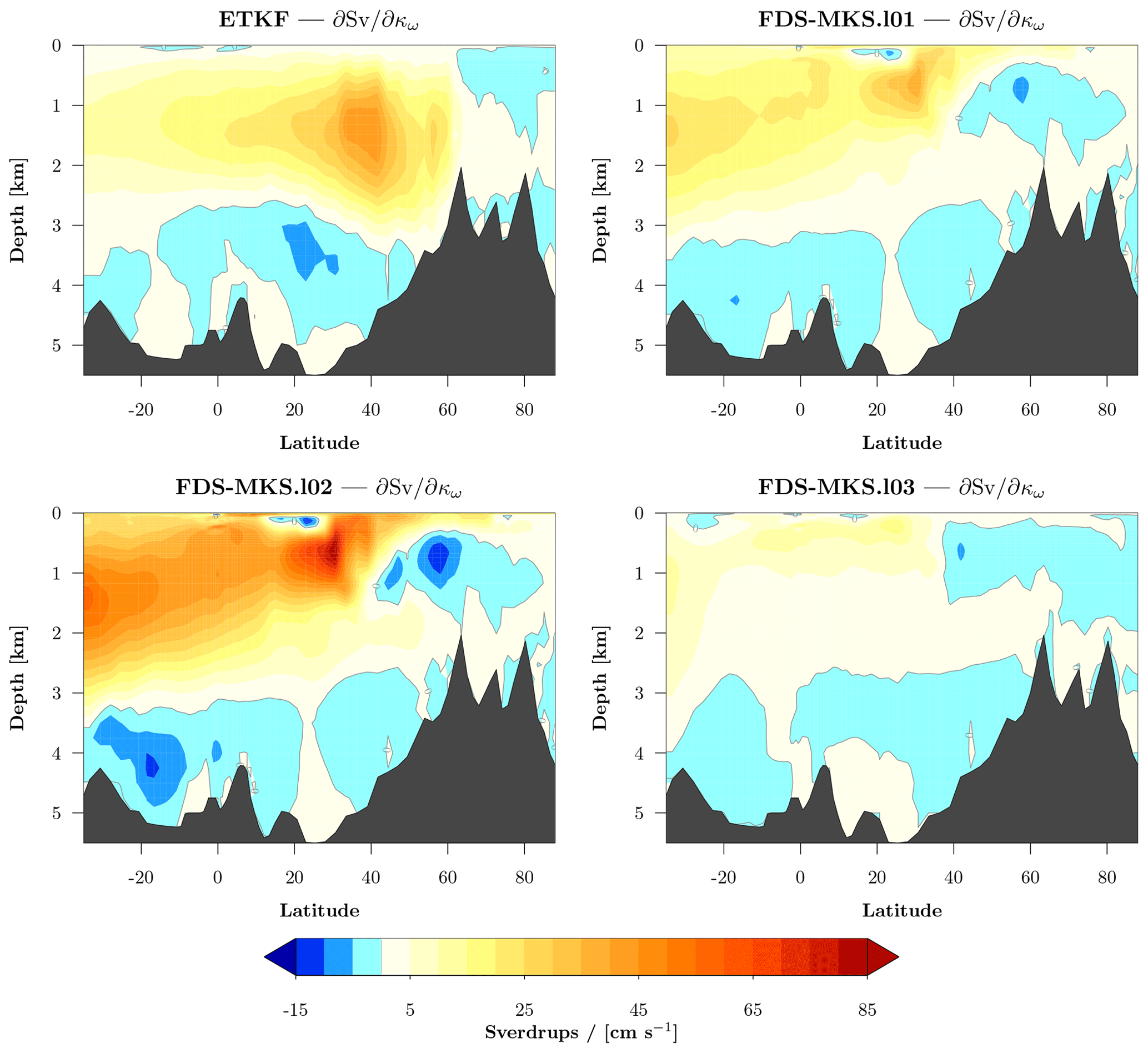
Figure 7CESM experiment. Sensitivity of the Atlantic meridional overturning circulation (AMOC) to the ocean background vertical diffusion parameter (κω; POP2.bckgrnd_vdc1) in the ocean model estimated as ensemble sensitivity (from the ETKF background ensemble) and local FDS along the iterations of the three-step FDS-MKS.
As a last related example, Fig. 8 shows the sensitivity of some atmospheric variables to the same ocean background vertical diffusion parameter obtained from the ensemble sensitivity (for ETKF) and the first iteration of the FDS schemes (for FDS-IKS or FDS-MKS). The atmospheric variables are the 2 m air temperature (T2M), convective precipitation (PRECC), large-scale precipitation (PRECL), and total cloud cover (CLDTOT). In general, the four variables show some similarities between the ensemble sensitivities and the FDS but also some important differences. The 2 m air temperature sensitivity patterns are in a rather good agreement, with the ensemble sensitivity mostly resembling a smoothed version of the FDS, although also diverging in some areas such as northern Europe around Scandinavia and northern Asia. The relatively amplified sensitivity seen in the FDS plot also leads to some areas reaching a negative sensitivity in the FDS estimates, while having a low but still positive sensitivity in the ensemble plot, as happens to the south of 30∘ S in the Atlantic and Pacific around South America. Part of the differences is certainly due to the more global sensitivity explored in the ensemble, but it is also pending to see how different perturbation sizes in the FDS would have affected its sensitivity pattern and amplitude. With different patterns, a similar comparison can be done between the ensemble sensitivity and the FDS for convective precipitation, which in both cases shows a higher (in absolute values) sensitivity in the tropics and a rather reasonable agreement, although it is very different in the tropical eastern Pacific to the south of the Equator. The tropical climate may indicate the indirect effects of changes in evaporation, atmospheric convection, and cloud formation. There are higher differences for large-scale precipitation, although some similarities are also present, such as the trough stretching from the tropical eastern Pacific, across South America, to the south of Africa or the high sensitivity in the tropical western Pacific. The total cloud cover finds a substantial difference between the sensitivity plots above ∼30∘ N. However, the delineation (0 isoline) between the negative and positive values is substantially similar in both sensitivities. In general, despite the differences between the two sensitivity estimates (due to the different exploration of the control vector space), the similarities, along with the reasonable sensitivity patterns shown for the AMOC for the same ocean parameter κω, point to the usefulness of the strongly coupled assimilation for the low-frequency climate analysis, in which observations from one component of the Earth system are allowed to influence the state and parameters for a different component.
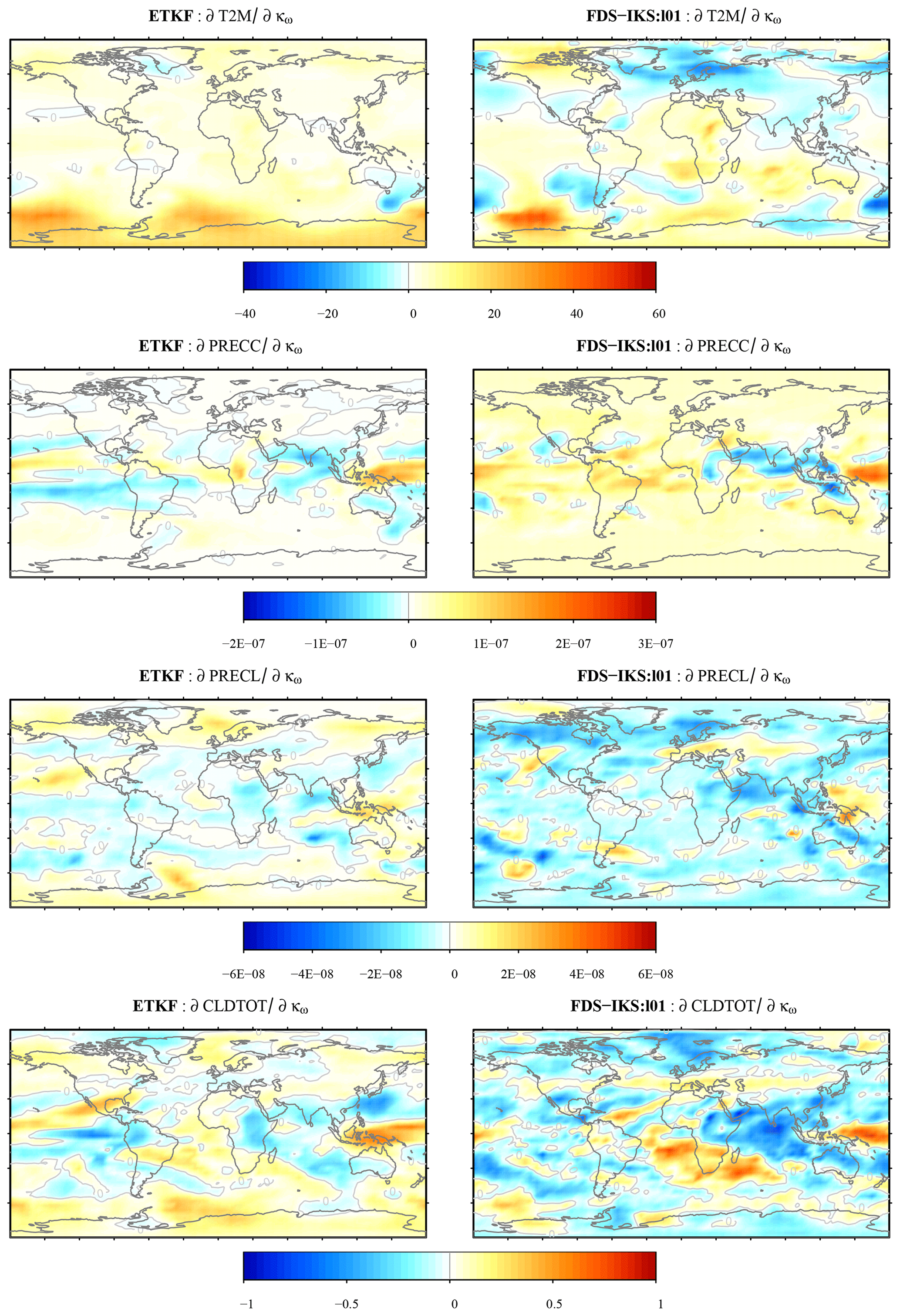
Figure 8CESM experiment. Sensitivity of several atmospheric variables to the ocean background vertical diffusion parameter (κω; POP2.bckgrnd_vdc1) in the ocean model estimated as ensemble sensitivity (from the ETKF background ensemble) and the local FDS for the first iteration of both the FDS-MKS and the FDS-IKS. The atmospheric variables are 2 m air temperature (T2M), total convective precipitation rate (PRECC), large-scale (stable) precipitation rate (PRECL), and vertically integrated total cloud cover (CLDTOT). Isolines at value 0 shown in grey.
An important last consideration is that the assimilation will just attempt to minimize (or get the first moments of) the cost function. So the assumed background statistics in the cost function are instrumental in controlling the control vector increments in the assimilation and the resulting climate field reconstruction (CFR). In this synthetic experiment the source of errors is known, and we assume a perfect-model framework except for the assumed uncertainties in the chosen control vector. However, in a real applied situation the real model errors are unknown. As described in the Introduction, the control vector increments will compensate for non-accounted errors. Although the minimization can highly reduce the value of a cost function and improve the corresponding CFR, it does not necessarily imply that updated parameters for the model physics (or their moments), as part of the control vector, actually correspond to improved (extrapolable) model physics. For example, the use of the posterior model parameters can potentially lead to improved climate simulations for other prospective climatic conditions, but not necessarily. Thus, it is important to distinguish between the use of the assimilation methods for CFR including model parameters as control variables and the trust one can have in the estimated model parameters for future climate projections under very different climatic conditions. A fair caveat was recently given by Dommenget and Rezny (2017) regarding the use of flux corrections as an alternative to parameter estimation in CGCMs. As they indicated, the compensating error risk when using parameter estimates for one specific observation dataset for future projections can be eliminated by using flux corrections instead to estimate the CFR. However, as flux corrections (with specific shapes) serve as a parametric way of expressing a model error, but also try to account for errors in boundary conditions (e.g. melting in a non-modelled ice sheet) which are specific for a climatic condition, the estimated flux corrections do not serve to improve the climate projections. All in all, our experiment with CESM is an example of a joint estimation of flux correction, model parameters, and forcing errors. The goal is to analyse the low-frequency past climate; at the very least, the divergence between the parameters for the model physics estimated for multi-decadal and longer past climate conditions and the values estimated for present conditions should serve to evaluate the reasons for the divergences, which points back to our introductory opening reference (Kageyama et al., 2018).
This study focuses on low-frequency climate field reconstruction (multi-decadal and longer timescales) with comprehensive deterministic Earth system models (ESMs). Given the enormous computational requirements for this class of models, we evaluate two iterative schemes based on reduced-order control vectors and the Kalman filter as assimilation approaches for climate field reconstruction. The schemes use an explicit representation of the background-error covariance matrix, and the Kalman gain is based on finite-difference sensitivity (FDS) experiments. As such, the schemes are computationally limited to the estimation of a low-dimensional control vector. The underlying assumption is so that a low-dimensional control vector and its background uncertainty, containing the most sensitive variables for a given climate, can encapsulate most of the modelled internal and external climate variability. The control vector can contain parameterized errors in initial conditions and parameters for the small-scale physics, as well as parameters for forcing and boundary condition errors (e.g. a bias in a time-varying radiative constituent). In general, it is expected that errors in initial conditions are a low sensitive input for the low-frequency model climate response. Thus, these would be generally excluded from the control vector, which makes it relatively easier to keep its low dimensionality.
The evaluated schemes are an FDS implementation of the iterative Kalman smoother (FDS-IKS, a Gauss–Newton scheme) and a so-called FDS-multistep Kalman smoother (FDS-MKS, based on repeated assimilation of the observations). We have conducted two assimilation experiments: (a) a simple 1-D energy balance model (Ebm1D; which has an adjoint code) with present-day surface air temperature from the NCEP/NCAR reanalysis data as a target and (b) a multi-decadal synthetic case with the Community Earth System Model (CESM v1.2, with no adjoint). The methodological description and the first experiment serve to show that, under a strong-constraint minimization and perfect-model framework, the FDS-IKS should converge to the same minimum as incremental 4D-Var. Actually, in this experiment, the FDS-IKS converges substantially faster than 4D-Var and to the same minimum. The FDS-MKS does not theoretically converge to the same minimum (except for linear cases), but it is more stable than the FDS-IKS for poorly regularized cost functions.
In a second experiment with CESM, given the lack of an adjoint code, we included an ETKF (with m=60 ensemble members) and an ETKF with Gaussian anamorphosis (ETKF-GA), as a non-linear estimation approach alternative to 4D-Var, as benchmarking schemes. As far as the authors know, this is also the first time that the ETKF-GA is evaluated with a comprehensive ESM for past climate multi-decadal analysis. Regarding the cost function as a performance criterion, the ETKF-GA was not clearly better or worse than a standard ETKF. We have shown that the GA does not solve the strong non-linearities which sensitivities may find at some observations. A clear example is the North Atlantic SST. The results cannot be extrapolated, for example, to shorter-term climate analyses. Also, alternative anamorphosis strategies for low-frequency analysis could show an improvement in the assimilation due to the transformations. With relatively high perturbations, both FDS schemes resulted (with about half the computing cost) in lower cost function values than the ETKF and the ETKF-GA. We would expect more optimal (likely smaller) perturbations adapted to individual control variables to result in further improvement in the FDS schemes, mostly the FDS-IKS (which, according to the first experiment, should be less resilient to the perturbation size). Given the computational requirements of comprehensive ESMs and current HPCs, the experiments here indicate that the FDS iterated schemes can be a relatively efficient strategy for dealing with the non-linear relation between model inputs and paleoclimate proxy observations. This non-linearity is introduced by both the ESM and the forward operators (proxy system models in general). From these experiments, the general impression is that one would choose the FDS-IKS over FDS-MKS as it should converge to the same minimum as incremental 4D-Var under the given assumptions. However, the experiments indicate that initially damped increments, such as those with FDS-MKS, should improve the convergence. So, FDS-MKS iterations (one or two) could be used initially to update the control vector estimate and then be followed by FDS-IKS iterations (with the background covariance). Note that, alternatively, a linear search along the same direction provided by the FDS-IKS could also be possible. An evaluation of further possibilities is needed.
This study is a first attempt to use the described iterated schemes for assimilation with comprehensive ESMs and multi-decadal or longer timescales. It has provided the context of the problem, described the schemes, and conducted preliminary experiments. The study is limited by the same computational constraint that motivates it. Further study is clearly needed before this type of scheme can be applied soundly for low-frequency past climate analyses in real cases. This would at least include sensitivity analyses for control vector design, error compensation analyses, and model error (Sakov and Bocquet, 2018; Sakov et al., 2018). In addition, other paleo-assimilation issues summarized in the paper regarding model–data comparison and observational error characteristics, whose discussion goes beyond the scope of this study, need to be considered.
In this paper we used Ebm1D-ad v1.0.0, a version of the Ebm1D model including the adjoint code available at https://github.com/andre-paul/ebm1d-ad/tree/v1.0.0 (Paul, 2018). We used the public release of CESM v1.2.2, available through http://www.cesm.ucar.edu/models/cesm1.2 (last access: 1 June 2016). For the ensemble assimilation (ETKF and FDS Kalman smoothers), we used rDAF v1.0.0 as a core data assimilation framework within the R environment (R Core Team, 2018), available at https://github.com/garciapintado/rDAF/tree/v1.0.0 (García-Pintado, 2018a). For the specific interface for the models we used rdafEbm1D v1.0.0, available at https://github.com/garciapintado/rdafEbm1D/tree/v1.0.0 (García-Pintado, 2018b), and rdafCESM v1.0.0, available at https://github.com/garciapintado/rdafCESM/tree/v1.0.0 (García-Pintado, 2018c).
Here we give tabulated details and a summary of the convergence tests for the finite-difference schemes in the experiment with the model Ebm1D. Table A1 shows the convergence results. The tests have the naming code SCN_FFFFxIT_mNN_sdfacSSSS, with the following terms.
-
SCN: weight scenario for the cost term Jo in Eq. (35), with the following alternatives:
-
PD1: present-day scenario,
-
PD2: present-day scenario,
-
PD3: present-day scenario,
-
-
FFFF: assimilation scheme, with the following options:
-
pIKS: FDS-IKS
-
pMKS: FDS-MKS
-
-
IT: Number of iterations. Fixed for FDS-MKS. Maximum for FDS-IKS.
-
NN: number of perturbations mθ for each control variable. Including the estimate at each loop, the total ensemble size is , where q is the dimension of the control vector.
-
SSSS: 1000×SDfac. For example, SSSS code “0010” indicates SDfac =0.010. For mθ=1 (forward finite differences), the perturbation of each control variable for sensitivity estimation is , where is the standard deviation of the control variable. For mθ>1, perturbations for each control variable are drawn from .
Table A11-D energy balance model experiment. Cost function values for the tests with the FDS schemes*.
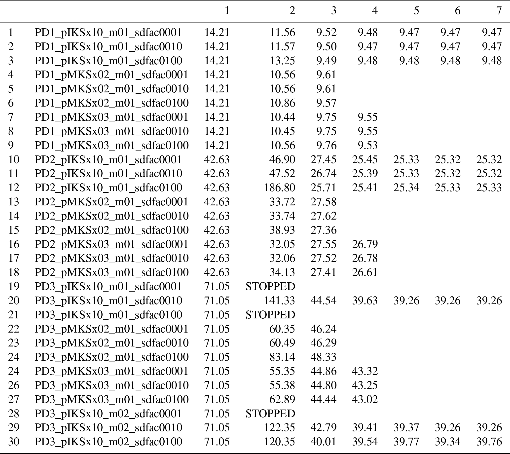
* Background cost function value in first column, followed by values along iterations. STOPPED indicates non-convergence (unstable model integration).
The tests are considered to evaluate the resilience of the Gauss–Newton scheme (FDS-IKS) to high perturbations and decreasing regularization and how this affects the relative performance of the Gauss–Newton scheme versus the multistep scheme (FDS-MKS). Specific cost function values are to be compared quantitatively only within a specific weight scenario (PD1, PD2, or PD3). For higher weights (being PD3 the highest), the effect of regularization by the background term decreases, which increases the chances of the FDS-IKS not converging (STOPPED tests due to unstable model integrations). Further tests (not shown) with even higher observational weight than PD3 are more and more difficult for the FDS-IKS to converge.
Scheduling of computing resources is more uncertain with the FDS-IKS than with the FDS-MKS. However, regarding this experiment and model, when the FDS-IKS converges, the values of the cost function are lower than those of the corresponding FDS-MKS test. This happens for FDS-MKS with either two or three iterations. Thus, with adequate regularization, the FDS-IKS is favoured. With decreasing observation uncertainty (decreasing regularization), the FDS-MKS stays more stable (see PD2 and PD3 tests). Still, for low regularization (PD3) the FDS-MKS cost function values (∼46 for the two-step FDS-MKS and ∼43 for the three-step FDS-MKS) are higher than those by the FDS-IKS when it converges ( ∼39). The three-step FDS-MKS always obtains lower values that the corresponding two-step FDS-MKS, but (generally) the differences are not very high. Interestingly, in some instances, the second step of the three-step FDS-MKS already has lower cost function values than the final estimation of the two-step FDS-MKS. This effect increases with decreased regularization. When the FDS-IKS starts to have convergence problems (see PD3 tests), increasing the ensemble size by conducting two perturbations per parameter (akin to central finite differences) makes the FDS-IKS more stable. A higher number of perturbations (not shown) makes the scheme more stable, but this would not be practical for long-term analyses with comprehensive ESMs.
B1 Example of well-behaved Gaussian anamorphosis
As an example, Fig. B1 shows scatterplots between the parameter CAM.cldfrc_rhminl and SST for a location in the South Pacific in the limits of the Antarctic circumpolar current. The location is shown in Fig. 5. Scatterplots are shown for the original variables and those with a Gaussian anamorphosis transformation. As opposed to Fig. 4, in this case Gaussianity is improved in the anamorphosed SST, and also the scatterplots show that an implicit pseudolinearization appears between the two anamorphosed variables, mostly as a result of the SST transformation.
B2 Convergence of the FDS-IKS and posterior standard deviations
Table B1 shows the convergence of the cost function for the FDS-IKS in the CESM experiment. Table B2 shows the posterior standard deviations of the control vector for the iterated FDS schemes, as well as for the ETKF and the ETKF-GA.
Table B1CESM parameter estimation: convergence of FDS-IKS cost function.
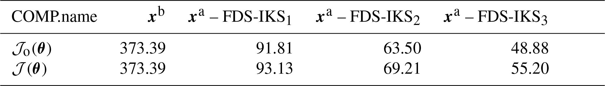
1 Units as described in Table 1. 2 Subindices in FDS-IKS refer to loop number. First iteration, FDS-IKS1, is also the FDS-EKS.
Table B2CESM posterior standard deviation in control variables1.
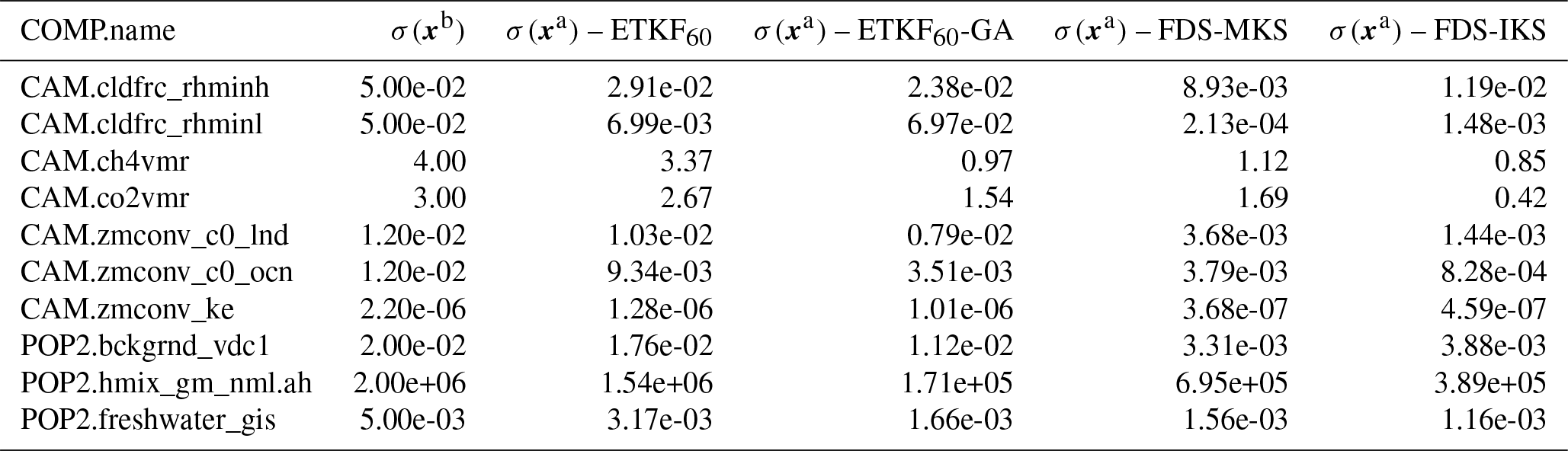
1 Units as described in Table 1. 2 ETKF subindex indicates the ensemble size.

Figure B1CESM experiment. Example of Gaussian anamorphosis transformation in a control variable (minimum relative humidity for high stable cloud formation) and the sea surface temperature (SST) for both the model equivalent of the observations and the observation (transformation details in text) at a location (245.3∘E, 54.91∘S) in the South Pacific (location shown in 5). Further description of symbols is as in Fig. 4.
AP wrote the code for Ebm1D-ad. JGP wrote the code for rDAF, rdafEbm1d, and rdafCESM. Both authors were involved in the experiments and contributed to the writing of the paper.
The authors declare that they have no conflict of interest.
This work has been supported by the German Federal Ministry of Education and
Research (BMBF) as a Research for Sustainability initiative (FONA) through
the Palmod project (01LP1511D). The authors acknowledge the North-German
Supercomputing Alliance (HLRN) for providing HPC resources that have
contributed to the research results reported in this paper. We thank two
anonymous reviewers for their positive comments, which have been very helpful
in improving the paper.
The article processing
charges for this open-access
publication were covered by the
University of Bremen.
Edited by: James
Annan
Reviewed by: two anonymous referees
Acevedo, W., Fallah, B., Reich, S., and Cubasch, U.: Assimilation of pseudo-tree-ring-width observations into an atmospheric general circulation model, Clim. Past, 13, 545–557, https://doi.org/10.5194/cp-13-545-2017, 2017. a, b
Amezcua, J. and Leeuwen, P. J. V.: Gaussian anamorphosis in the analysis step of the EnKF: A joint state-variable/observation approach, Tellus A, 66, 23493, https://doi.org/10.3402/tellusa.v66.23493, 2014. a, b, c, d, e, f
Annan, J. D., Hargreaves, J. C., Edwards, N. R., and R, M.: Parameter estimation in an intermediate complexity Earth System Model using an ensemble Kalman filter, Ocean Modell., 8, 135–154, https://doi.org/10.1016/j.ocemod.2003.12.004, 2005a. a, b
Annan, J. D., Lunt, D. J., Hargreaves, J. C., and Valdes, P. J.: Parameter estimation in an atmospheric GCM using the Ensemble Kalman Filter, Nonlin. Processes Geophys., 12, 363–371, https://doi.org/10.5194/npg-12-363-2005, 2005b. a, b, c, d, e
Arakawa, A.: The cumulus parameterization problem: Past, present, and future, J. Climate, 17, 2493–2525, https://doi.org/10.1175/1520-0442(2004)017<2493:RATCPP>2.0.CO;2, 2004. a
Arakawa, A., Jung, J.-H., and Wu, C.-M.: Toward unification of the multiscale modeling of the atmosphere, Atmos. Chem. Phys., 11, 3731–3742, https://doi.org/10.5194/acp-11-3731-2011, 2011. a
Bannister, R. N.: A review of operational methods of variational and ensemble-variational data assimilation, Q. J. Roy. Meteor. Soc., 143, 607–633, https://doi.org/10.1002/qj.2982, 2017. a, b
Béal, D., Brasseur, P., Brankart, J.-M., Ourmières, Y., and Verron, J.: Characterization of mixing errors in a coupled physical biogeochemical model of the North Atlantic: implications for nonlinear estimation using Gaussian anamorphosis, Ocean Sci., 6, 247–262, https://doi.org/10.5194/os-6-247-2010, 2010. a, b
Bell, B. M.: The Iterated Kalman Smoother as a Gauss–Newton Method, SIAM J. Optimiz., 4, 626–636, https://doi.org/10.1137/0804035, 1994. a, b, c
Bell, B. M. and Cathey, F. W.: The iterated Kalman filter update as a Gauss-Newton method, IEEE T. Automat. Contr., 38, 294–297, https://doi.org/10.1109/9.250476, 1993. a
Bertino, L., Evensen, G., and Wackernagel, H.: Sequential Data Assimilation Techniques in Oceanography, Int. Stat. Rev., 71, 223–241, https://doi.org/10.1111/j.1751-5823.2003.tb00194.x, 2003. a, b
Bishop, C. H., Etherton, B. J., and Majumdar, S. J.: Adaptive Sampling with the Ensemble Transform Kalman Filter. Part I: Theoretical aspects, Mon. Weather Rev., 129, 420–436, https://doi.org/10.1175/1520-0493(2001)129<0420:ASWTET>2.0.CO;2, 2001. a
Bocquet, M. and Sakov, P.: Joint state and parameter estimation with an iterative ensemble Kalman smoother, Nonlin. Processes Geophys., 20, 803–818, https://doi.org/10.5194/npg-20-803-2013, 2013. a, b
Bocquet, M. and Sakov, P.: An iterative ensemble Kalman smoother, Q. J. Roy. Meteor. Soc., 140, 1521–1535, https://doi.org/10.1002/qj.2236, 2014. a, b, c
Chen, Y. and Oliver, D. S.: Ensemble Randomized Maximum Likelihood Method as an Iterative Ensemble Smoother, Math. Geosci., 44, 1–26, https://doi.org/10.1007/s11004-011-9376-z, 2012. a
Chìles, J.-P. and Delfiner, P.: Geostatistics: Modeling spatial uncertainty, 2nd edition, John Wiley & Sons, Ltd., 2012. a
Christiansen, B. and Ljungqvist, F. C.: Challenges and perspectives for large-scale temperature reconstructions of the past two millennia, Rev. Geophys., 50, 40–96, https://doi.org/10.1002/2016RG000521, 2017. a
Chuang, C. C., Kelly, J. T., Boyle, J. S., and Xie, S.: Sensitivity of aerosol indirect effects to cloud nucleation and autoconversion parameterizations in short-range weather forecasts during the May 2003 aerosol IOP, J. Adv. Model. Earth Sy., 4, m09001, https://doi.org/10.1029/2012MS000161, 2012. a
Cohn, S. E.: An Introduction to Estimation Theory (Special Issue, Data Assimilation in Meteology and Oceanography: Theory and Practice), J. Meteorol. Soc. Jpn., 75, 257–288, https://doi.org/10.2151/jmsj1965.75.1B_257, 1997. a
Courtier, P., Thépaut, J.-N., and Hollingsworth, A.: A strategy for operational implementation of 4D-Var, using an incremental approach, Q. J. Roy. Meteor. Soc., 120, 1367–1387, https://doi.org/10.1002/qj.49712051912, 1994. a
Covey, C., Lucas, D. D., Tannahill, J., Garaizar, X., and Klein, R.: Efficient screening of climate model sensitivity to a large number of perturbed input parameters, J. Adv. Model. Earth Sy., 5, 598–610, https://doi.org/10.1002/jame.20040, 2013. a
Dail, H. and Wunsch, C.: Dynamical Reconstruction of Upper-Ocean Conditions in the Last Glacial Maximum Atlantic, J. Climate, 27, 807–823, https://doi.org/10.1175/JCLI-D-13-00211.1, 2014. a
Dee, S. G., Steiger, N. J., Emile-Geay, J., and Hakim, G. J.: On the utility of proxy system models for estimating climate states over the common era, J. Adv. Model. Earth Sy., 8, 1164–1179, https://doi.org/10.1002/2016MS000677, 2016. a
Delworth, T. L., Manabe, S., and Stouffer, R. J.: Multidecadal climate variability in the Greenland Sea and surrounding regions: A coupled model simulation, Geophys. Res. Lett., 24, 257–260, https://doi.org/10.1029/96GL03927, 1997. a, b
Dennis, Jr., J. E. and Schnabel, R. B.: Numerical Methods for Unconstrained Optimization and Nonlinear Equations (Classics in Applied Mathematics, 16), Soc for Industrial & Applied Math, 1996. a
Deutsch, C. V. and Journel, A. G.: GSLIB: Geostatistical Software Library and User's Guide, Oxford UP, NY, 1998. a
Dirren, S. and Hakim, G. J.: Toward the assimilation of time-averaged observations, Geophys. Res. Lett., 32, L04804, https://doi.org/10.1029/2004GL021444, 2005. a
Dommenget, D. and Rezny, M.: A Caveat Note on Tuning in the Development of Coupled Climate Models, J. Adv. Model. Earth Sy., 10, 78–97, https://doi.org/10.1002/2017MS000947, 2017. a
Doron, M., Brasseur, P., and Brankart, J.-M.: Stochastic estimation of biogeochemical parameters of a 3D ocean coupled physical-biogeochemical model: Twin experiments, J. Marine Syst., 87, 194–207, https://doi.org/10.1016/j.jmarsys.2011.04.001, 2011. a
Dubinkina, S., Goosse, H., Sallaz-Damaz, Y., Crespin, E., and Crucifix, M.: Testing a particle filter to reconstruct climate changes over the past centuries, Int. J. Bifurcat. Chaos, 21, 3611–3618, https://doi.org/10.1142/S0218127411030763, 2011. a
Emerick, A. A. and Reynolds, A. C.: Ensemble smoother with multiple data assimilation, Comput. Geosci., 55, 3–15, https://doi.org/10.1016/j.cageo.2012.03.011, 2013. a
Evans, M., Tolwinski-Ward, S., Thompson, D., and Anchukaitis, K.: Applications of proxy system modeling in high resolution paleoclimatology, Quaternary Sci. Rev., 76, 16–28, https://doi.org/10.1016/j.quascirev.2013.05.024, 2013. a
Evensen, G.: Inverse methods and data assimilation in nonlinear ocean models, Physica D, 77, 108–129, https://doi.org/10.1016/0167-2789(94)90130-9, 1994. a, b
Friedland, B.: Treatment of bias in recursive filtering, IEEE T. Automat. Contr., 14, 359–367, https://doi.org/10.1109/TAC.1969.1099223, 1969. a
Gao, G. and Reynolds, A. C.: An Improved Implementation of the LBFGS Algorithm for Automatic History Matching, SPE J., 11, 5–17, https://doi.org/10.2118/90058-PA, 2006. a, b
García-Pintado, J.: rDAF v1.0.0: R data assimilation framework, https://doi.org/10.5281/zenodo.1489131, 2018a. a, b, c
García-Pintado, J.: rdafEbm1D v1.00: rDAF interface for Ebm1D, https://doi.org/10.5281/zenodo.1489133, 2018b. a, b
García-Pintado, J.: rdafCESM v1.0.0: rDAF interface for CESM, https://doi.org/10.5281/zenodo.1489135, 2018c. a, b
García-Pintado, J., Neal, J. C., Mason, D. C., Dance, S. L., and Bates, P. D.: Scheduling satellite-based SAR acquisition for sequential assimilation of water level observations into flood modelling, J. Hydrol., 495, 252–266, https://doi.org/10.1016/j.jhydrol.2013.03.050, 2013. a
Gent, P. R. and McWilliams, J. C.: Isopycnal Mixing in Ocean Circulation Models, J. Phys. Oceanogr., 20, 150–155, https://doi.org/10.1175/1520-0485(1990)020<0150:IMIOCM>2.0.CO;2, 1990. a, b
Giering, R. and Kaminski, T.: Recipes for Adjoint Code Construction, ACM T. Math. Software, 24, 437–474, https://doi.org/10.1145/293686.293695, 1998. a
Giering, R., Kaminski, T., and Slawig, T.: Generating Efficient Derivative Code with TAF, Future Gener. Comp. Sy., 21, 1345–1355, https://doi.org/10.1016/j.future.2004.11.003, 2005. a
Gilbert, J. C. and Lemaréchal, C.: Some numerical experiments with variable-storage quasi-Newton algorithms, Math. Program., 45, 407–435, https://doi.org/10.1007/BF01589113, 1989. a, b
Goosse, H.: An additional step toward comprehensive paleoclimate reanalyses, J. Adv. Model. Earth Sy., 8, 1501–1503, https://doi.org/10.1002/2016MS000739, 2016. a
Gregory, J. M. and Tailleux, R.: Kinetic energy analysis of the response of the Atlantic meridional overturning circulation to CO2-forced climate change, Clim. Dynam., 37, 893–914, https://doi.org/10.1007/s00382-010-0847-6, 2011. a
Gu, Y. and Oliver, D. S.: An Iterative Ensemble Kalman Filter for Multiphase Fluid Flow Data Assimilation, Society of Petroleum Engineers, 12, 438–446, https://doi.org/10.2118/108438-PA, 2007. a
Hack, J. J.: Parameterization of moist convection in the National Center for Atmospheric Research community climate model (CCM2), J. Geophys. Res.-Atmos., 99, 5551–5568, https://doi.org/10.1029/93JD03478, 1994. a
Hakim, G. J., Emile-Geay, J., Steig, E. J., Noone, D., Anderson, D. M., Tardif, R., Steiger, N., and Perkins, W. A.: The last millennium climate reanalysis project: Framework and first results, J. Geophys. Res.-Atmos., 121, 6745–6764, https://doi.org/10.1002/2016JD024751, 2016JD024751, 2016. a
Hargreaves, J. and Annan, J.: Assimilation of paleo-data in a simple Earth system model, Clim. Dynam., 19, 371–381, https://doi.org/10.1007/s00382-002-0241-0, 2002. a
Hargreaves, J. C., Paul, A., Ohgaito, R., Abe-Ouchi, A., and Annan, J. D.: Are paleoclimate model ensembles consistent with the MARGO data synthesis?, Clim. Past, 7, 917–933, https://doi.org/10.5194/cp-7-917-2011, 2011. a
Hartmann, D. L.: Global physical climatology, Academic Press, San Diego, 1994. a
Hartmann, D. L. and Short, D. A.: On the Role of Zonal Asymmetries in Climate Change, J. Atmos. Sci., 36, 519–528, https://doi.org/10.1175/1520-0469(1979)036<0519:OTROZA>2.0.CO;2, 1979. a
Holland, M. M., Blanchard-Wrigglesworth, E., Kay, J., and Vavrus, S.: Initial-value predictability of Antarctic sea ice in the Community Climate System Model 3, Geophys. Res. Lett., 40, 2121–2124, https://doi.org/10.1002/grl.50410, 2013. a
Ide, K., Courtier, P., Ghill, M, and Lorenc, A. C.: Unified notation for Data Assimilation: operational, sequential and variational, J. Meteorol. Soc. Jpn., 75, 181–189, 1997. a
Janjić, T., Bormann, N., Bocquet, M., Carton, J. A., Cohn, S. E., Dance, S. L., Losa, S. N., Nichols, N. K., Potthast, R., Waller, J. A., and Weston, P.: On the representation error in data assimilation, Q. J. Roy. Meteor. Soc., 144, 1257–1278, https://doi.org/10.1002/qj.3130, 2017. a
Jazwinski, A. H.: 8 Applications of Linear Theory, in: Stochastic Processes and Filtering Theory, edited by: Jazwinski, A. H., vol. 64, Mathematics in Science and Engineering, Elsevier, 266–331, 1970. a, b
Jungclaus, J. H., Bard, E., Baroni, M., Braconnot, P., Cao, J., Chini, L. P., Egorova, T., Evans, M., González-Rouco, J. F., Goosse, H., Hurtt, G. C., Joos, F., Kaplan, J. O., Khodri, M., Klein Goldewijk, K., Krivova, N., LeGrande, A. N., Lorenz, S. J., Luterbacher, J., Man, W., Maycock, A. C., Meinshausen, M., Moberg, A., Muscheler, R., Nehrbass-Ahles, C., Otto-Bliesner, B. I., Phipps, S. J., Pongratz, J., Rozanov, E., Schmidt, G. A., Schmidt, H., Schmutz, W., Schurer, A., Shapiro, A. I., Sigl, M., Smerdon, J. E., Solanki, S. K., Timmreck, C., Toohey, M., Usoskin, I. G., Wagner, S., Wu, C.-J., Yeo, K. L., Zanchettin, D., Zhang, Q., and Zorita, E.: The PMIP4 contribution to CMIP6 – Part 3: The last millennium, scientific objective, and experimental design for the PMIP4 past1000 simulations, Geosci. Model Dev., 10, 4005–4033, https://doi.org/10.5194/gmd-10-4005-2017, 2017. a
Kageyama, M., Laîné, A., Abe-Ouchi, A., Braconnot, P., Cortijo, E., Crucifix, M., de Vernal, A., Guiot, J., Hewitt, C., Kitoh, A., Kucera, M., Marti, O., Ohgaito, R., Otto-Bliesner, B., Peltier, W., Rosell-Melé, A., Vettoretti, G., Weber, S., and Yu, Y.: Last Glacial Maximum temperatures over the North Atlantic, Europe and western Siberia: a comparison between PMIP models, MARGO sea-surface temperatures and pollen-based reconstructions, Quaternary Sci. Rev., 25, 2082–2102, https://doi.org/10.1016/j.quascirev.2006.02.010, 2006. a
Kageyama, M., Braconnot, P., Harrison, S. P., Haywood, A. M., Jungclaus, J. H., Otto-Bliesner, B. L., Peterschmitt, J.-Y., Abe-Ouchi, A., Albani, S., Bartlein, P. J., Brierley, C., Crucifix, M., Dolan, A., Fernandez-Donado, L., Fischer, H., Hopcroft, P. O., Ivanovic, R. F., Lambert, F., Lunt, D. J., Mahowald, N. M., Peltier, W. R., Phipps, S. J., Roche, D. M., Schmidt, G. A., Tarasov, L., Valdes, P. J., Zhang, Q., and Zhou, T.: The PMIP4 contribution to CMIP6 – Part 1: Overview and over-arching analysis plan, Geosci. Model Dev., 11, 1033–1057, https://doi.org/10.5194/gmd-11-1033-2018, 2018. a, b
Kalnay, E., Kanamitsu, M., Kistler, R., Collins, W., Deaven, D., Gandin, L., Iredell, M., Saha, S., White, G., Woollen, J., Zhu, Y., Leetmaa, A., Reynolds, R., Chelliah, M., Ebisuzaki, W., Higgins, W., Janowiak, J., Mo, K. C., Ropelewski, C., Wang, J., Jenne, R., and Joseph, D.: The NCEP/NCAR 40-Year Reanalysis Project, B. Am. Meteor. Soc., 77, 437–471, https://doi.org/10.1175/1520-0477(1996)077<0437:TNYRP>2.0.CO;2, 1996. a
Klein, F. and Goosse, H.: Reconstructing East African rainfall and Indian Ocean sea surface temperatures over the last centuries using data assimilation, Clim. Dynam., 50, 3909–3929, https://doi.org/10.1007/s00382-017-3853-0, 2017. a
Köhler, P., Nehrbass-Ahles, C., Schmitt, J., Stocker, T. F., and Fischer, H.: A 156 kyr smoothed history of the atmospheric greenhouse gases CO2, CH4, and N2O and their radiative forcing, Earth Syst. Sci. Data, 9, 363–387, https://doi.org/10.5194/essd-9-363-2017, 2017. a, b
Kurahashi-Nakamura, T., Paul, A., and Losch, M.: Dynamical reconstruction of the global ocean state during the Last Glacial Maximum, Paleoceanography, 32, 326–350, https://doi.org/10.1002/2016PA003001, 2017. a, b
Large, W. G., McWilliams, J. C., and Doney, S. C.: Oceanic vertical mixing: A review and a model with a nonlocal boundary layer parameterization, Rev. Geophys., 32, 363–403, https://doi.org/10.1029/94RG01872, 1994. a
Lawless, A. S.: Variational data assimilation for very large environmental problems, in: Large Scale Inverse Problems, in: Radon series on computational and applied mathematics, edited by: Cullen, M., Freitag, M. A., Kindermann, S., and Scheichl, R., De Gruyter, Berlin, 13, 55–90, 2013. a
Lawless, A. S., Gratton, S., and Nichols, N. K.: An investigation of incremental 4D-Var using non-tangent linear models, Q. J. Roy. Meteor. Soc., 131, 459–476, https://doi.org/10.1256/qj.04.20, 2005. a, b
Liu, C., Xiao, Q., and Wang, B.: An Ensemble-Based Four-Dimensional Variational Data Assimilation Scheme. Part I: Technical Formulation and Preliminary Test, Mon. Weather Rev., 136, 3363–3373, https://doi.org/10.1175/2008MWR2312.1, 2008. a
Livings, D. M., Dance, S. L., and Nichols, N. K.: Unbiased Ensemble Square Root Filters, Physica D, 237, 1021–1028, https://doi.org/10.1016/j.physd.2008.01.005, 2008. a
Lorenc, A. C.: Analysis methods for numerical weather prediction, Q. J. Roy. Meteor. Soc., 112, 1177–1194, https://doi.org/10.1002/qj.49711247414, 1986. a, b
Lorenc, A. C.: Recommended nomenclature for EnVar data assimilation methods, in: WGNE Blue Book Research Activities in Atmospheric and Oceanic Modelling, section 01: 7–8, WMO: Geneva, Switzerland, 2013. a
Marchal, O., Waelbroeck, C., and de Verdière, A. C.: On the Movements of the North Atlantic Subpolar Front in the Preinstrumental Past, J. Climate, 29, 1545–1571, https://doi.org/10.1175/JCLI-D-15-0509.1, 2016. a
Marchi, S., Fichefet, T., Goosse, H., Zunz, V., Tietsche, S., Day, J. J., and Hawkins, E.: Reemergence of Antarctic sea ice predictability and its link to deep ocean mixing in global climate models, Clim. Dynam., https://doi.org/10.1007/s00382-018-4292-2, online first, 2018. a
MARGO Project Members: Constraints on the magnitude and patterns of ocean cooling at the Last Glacial Maximum, Nat. Geosci., 2, 127–132, https://doi.org/10.1038/ngeo411, 2009. a, b, c, d
Matheron, G.: Le krigeage disjunctive, Intern. Note N-360, Centre de Géostatistique, Ecole des Mines de Paris, Paris, France, 40 pp., 1973. a
Meehl, G. A., Arblaster, J. M., Bitz, C. M., Chung, C. T. Y., and Teng, H.: Antarctic sea-ice expansion between 2000 and 2014 driven by tropical Pacific decadal climate variability, Nat. Geosci., 9, 590–596, https://doi.org/10.1038/ngeo2751, 2016. a
Neale, R. B., Richter, R., Conley, A., Park, S., Lauritzen, P., Gettelman, A., Williamson, D., Rash, P., Vavrus, S., Taylor, M., Collins, W., Zhang, M., and Lin, S.-J.: Description of the NCAR Community Atmosphere Model (CAM4), Tech. Rep. NCAR/TN-485+STR, NCAR, 2011. a
North, G. R., Mengel, J. G., and Short, D. A.: Simple energy balance model resolving the seasons and the continents: Application to the astronomical theory of the ice ages, J. Geophys. Res.-Oceans, 88, 6576–6586, https://doi.org/10.1029/JC088iC11p06576, 1983. a, b
Oliver, D. S. and Chen, Y.: Improved initial sampling for the ensemble Kalman filter, Comput. Geosci., 13, 13–27, https://doi.org/10.1007/s10596-008-9101-2, 2008. a
Ortega, P., Lehner, F., Swingedouw, D., Masson-Delmotte, V., Raible, C. C., Casado, M., and Yiou, P.: A model-tested North Atlantic Oscillation reconstruction for the past millennium, Nature, 523, 71–74, https://doi.org/10.1038/nature14518, 2015. a
Ott, E., Hunt, B., Szunyogh, I., Zimin, A., Kostelich, E., Corazza, M., Kalnay, E., Patil, D., and Yorke, J.: A local ensemble Kalman filter for atmospheric data assimilation, Tellus A, 56, 415–428, https://doi.org/10.1111/j.1600-0870.2004.00076.x, 2004. a
Otto-Bliesner, B. L., Brady, E. C., Fasullo, J., Jahn, A., Landrum, L., Stevenson, S., Rosenbloom, N., Mai, A., and Strand, G.: Climate Variability and Change since 850 CE: An Ensemble Approach with the Community Earth System Model, B. Am. Meteorol. Soc., 97, 735–754, https://doi.org/10.1175/BAMS-D-14-00233.1, 2016. a, b
PAGES 2k-PMIP3 group: Continental-scale temperature variability in PMIP3 simulations and PAGES 2k regional temperature reconstructions over the past millennium, Clim. Past, 11, 1673–1699, https://doi.org/10.5194/cp-11-1673-2015, 2015. a
PAGES2k Consortium: A global multiproxy database for temperature reconstructions of the Common Era, Scientific data, 4, 170088, https://doi.org/10.1038/sdata.2017.88, 2017. a
Palmer, T. N. and Weisheimer, A.: Diagnosing the causes of bias in climate models – why is it so hard?, Geophys. Astro. Fluid, 105, 351–365, https://doi.org/10.1080/03091929.2010.547194, 2011. a
Paul, A.: Ebm1d-ad v1.0.0: 1D energy balance model of climate with automatic differentiation, https://doi.org/10.5281/zenodo.1489952, 2018. a, b
Paul, A. and Losch, M.: Perspectives of Parameter and State Estimation in Paleoclimatology, in: Climate Change: Inferences from Paleoclimate and Regional Aspects, edited by: Berger, A., Mesinger, F., and Sijacki, D., Springer Vienna, Vienna, 93–105, https://doi.org/10.1007/978-3-7091-0973-1_7, 2012. a, b
Paul, A. and Schäfer-Neth, C.: How to combine sparse proxy data and coupled climate models, Quaternary Sci. Revi., 24, 1095–1107, https://doi.org/10.1016/j.quascirev.2004.05.010, 2005. a
R Core Team: R: A Language and Environment for Statistical Computing, R Foundation for Statistical Computing, Vienna, Austria, available at: http://www.R-project.org/, last access: 2 July 2018. a, b
Rasch, P. J. and Kristjánsson, J. E.: A Comparison of the CCM3 Model Climate Using Diagnosed and Predicted Condensate Parameterizations, J. Climate, 11, 1587–1614, https://doi.org/10.1175/1520-0442(1998)011<1587:ACOTCM>2.0.CO;2, 1998. a
Sakov, P. and Bocquet, M.: Asynchronous data assimilation with the EnKF in presence of additive model error, Tellus A, 70, 1414545, https://doi.org/10.1080/16000870.2017.1414545, 2018. a
Sakov, P. and Oke, P. R.: Implications of the Form of the Ensemble Transformation in the Ensemble Square Root Filters, Mon. Weather Rev., 136, 1042–1053, https://doi.org/10.1175/2007MWR2021.1, 2008. a
Sakov, P., Evensen, G., and Bertino, L.: Asynchronous data assimilation with the EnKF, Tellus A, 62, 24–29, 2010. a
Sakov, P., Oliver, D. S., and Bertino, L.: An Iterative EnKF for Strongly Nonlinear Systems, Mon. Weather Rev., 140, 1988–2004, https://doi.org/10.1175/MWR-D-11-00176.1, 2012. a
Sakov, P., Jean-Matthieu, H., and Bocquet, M.: An iterative ensemble Kalman filter in the presence of additive model error, Q. J. Roy. Meteor. Soc., 144, 1297-1309, , https://doi.org/10.1002/qj.3213, 2018. a
Shapiro, S. S. and Wilk, M. B.: An analysis of variance test for normality (complete samples), Biometrika, 52, 591–611, https://doi.org/10.1093/biomet/52.3-4.591, 1965. a
Simon, E. and Bertino, L.: Application of the Gaussian anamorphosis to assimilation in a 3-D coupled physical-ecosystem model of the North Atlantic with the EnKF: a twin experiment, Ocean Sci., 5, 495–510, https://doi.org/10.5194/os-5-495-2009, 2009. a, b, c
Simon, E. and Bertino, L.: Gaussian anamorphosis extension of the DEnKF for combined state parameter estimation: Application to a 1D ocean ecosystem model, J. Marine Syst., 89, 1–18, https://doi.org/10.1016/j.jmarsys.2011.07.007, 2012. a, b, c
Smith, P. J., Dance, S. L., and Nichols, N. K.: A hybrid data assimilation scheme for model parameter estimation: Application to morphodynamic modelling, Comput. Fluids, 46, 436–441, https://doi.org/10.1016/j.compfluid.2011.01.010, 2011. a
Smith, R., Jones, P., Briegleb, B., Bryan, F., Danabasoglu, G., Dennis, J., Dukowicz, J., Eden, C., Fox-Kemper, B., Gent, P., Hecht, M., Jayne, S., Jochum, M., Large, W., Lindsay, K., Maltrud, M., Norton, N., Peacock, S., Vertenstein, M., and Yeager, S.: The Parallel Ocean Program (POP) Reference Manual, Ocean Component of the Community Climate System Model (CCSM) and Community Earth System Model (CESM), Tech. Rep. LAUR-10-01854, Los Alamos National Laboratory, Boulder, Colorado, 2010. a
Steiger, N. J., Hakim, G. J., Steig, E. J., Battisti, D. S., and Roe, G. H.: Assimilation of Time-Averaged Pseudoproxies for Climate Reconstruction, J. Climate, 27, 426–441, https://doi.org/10.1175/JCLI-D-12-00693.1, 2014. a
Tippett, M. K., Anderson, J. L., Bishop, C. H., Hamill, T. M., and Whitaker, J. S.: Ensemble Square Root Filters, Mon. Weather Rev., 131, 1485–1490, https://doi.org/10.1175/1520-0493(2003)131<1485:ESRF>2.0.CO;2, 2003. a
Waelbroeck, C., Kiefer, T., Dokken, T., Chen, M.-T., Spero, H., Jung, S., Weinelt, M., Kucera, M., and Paul, A.: Constraints on surface seawater oxygen isotope change between the Last Glacial Maximum and the Late Holocene, Quaternary Sci. Rev., 105, 102–111, https://doi.org/10.1016/j.quascirev.2014.09.020, 2014. a
Wang, X., Bishop, C. H., and Julier, S. J.: Which Is Better, an Ensemble of Positive–Negative Pairs or a Centered Spherical Simplex Ensemble?, Mon. Weather Rev., 132, 1590–1605, https://doi.org/10.1175/1520-0493(2004)132<1590:WIBAEO>2.0.CO;2, 2004. a
Weitzel, N., Wagner, S., Sjolte, J., Klockmann, M., Bothe, O., Andres, H., Tarasov, L., Rehfeld, K., Zorita, E., Widmann, M., Sommer, P., Schädler, G., Ludwig, P., Kapp, F., Jonkers, L., García-Pintado, J., Fuhrmann, F., Dolman, A., Dallmeyer, A., and Brücher, T.: Diving into the past – A paleo data-model comparison workshop on the Late Glacial and Holocene, B. Am. Meteorol. Soc., https://doi.org/10.1175/BAMS-D-18-0169.1, online first, 2018. a
Whitaker, J. S. and Hamill, T. M.: Ensemble Data Assimilation without Perturbed Observations, Mon. Weather Rev., 130, 1913–1924, https://doi.org/10.1175/1520-0493(2002)130<1913:EDAWPO>2.0.CO;2, 2002. a
Wu, Z., Reynolds, A., and Oliver, D.: Conditioning Geostatistical Models to Two-Phase Production Data, SPE J., 3, 142–155, https://doi.org/10.2118/56855-PA, 1999. a, b
Yang, B., Qian, Y., Lin, G., Leung, R., and Zhang, Y.: Some issues in uncertainty quantification and parameter tuning: a case study of convective parameterization scheme in the WRF regional climate model, Atmos. Chem. Phys., 12, 2409–2427, https://doi.org/10.5194/acp-12-2409-2012, 2012. a
Yang, B., Qian, Y., Lin, G., Leung, L. R., Rasch, P. J., Zhang, G. J., McFarlane, S. A., Zhao, C., Zhang, Y., Wang, H., Wang, M., and Liu, X.: Uncertainty quantification and parameter tuning in the CAM5 Zhang-McFarlane convection scheme and impact of improved convection on the global circulation and climate, J. Geophys. Res.-Atmos., 118, 395–415, https://doi.org/10.1029/2012JD018213, 2013. a, b
Zanchettin, D., Bothe, O., Lehner, F., Ortega, P., Raible, C. C., and Swingedouw, D.: Reconciling reconstructed and simulated features of the winter Pacific/North American pattern in the early 19th century, Clim. Past, 11, 939–958, https://doi.org/10.5194/cp-11-939-2015, 2015. a
Zhang, G. and McFarlane, N. A.: Sensitivity of climate simulations to the parameterization of cumulus convection in the Canadian climate centre general circulation model, Atmos.-Ocean, 33, 407–446, https://doi.org/10.1080/07055900.1995.9649539, 1995. a
Zhou, H., Gómez-Hernández, J. J., Franssen, H.-J. H., and Li, L.: An approach to handling non-Gaussianity of parameters and state variables in ensemble Kalman filtering, Adv. Water Resour., 34, 844–864, https://doi.org/10.1016/j.advwatres.2011.04.014, 2011. a
Zunz, V., Goosse, H., and Dubinkina, S.: Impact of the initialisation on the predictability of the Southern Ocean sea ice at interannual to multi-decadal timescales, Clim. Dynam., 44, 2267–2286, https://doi.org/10.1007/s00382-014-2344-9, 2015. a
- Abstract
- Introduction
- Assimilation schemes
- Experiment 1: 1-D energy balance model
- Experiment 2: CESM
- Conclusions
- Code availability
- Appendix A: Experiment 1: convergence analysis for finite-difference schemes
- Appendix B: Experiment 2
- Author contributions
- Competing interests
- Acknowledgements
- References