The Indian summer monsoon in MetUM-GOML2.0: effects of air–sea coupling and resolution

The fidelity of the simulated Indian summer monsoon is analysed in the UK Met Office Unified Model Global Ocean Mixed Layer configuration (MetUM-GOML2.0) in terms of its boreal summer mean state and propagation of the boreal summer intraseasonal oscillation (BSISO). The model produces substantial biases in mean June–September precipitation, especially over India, in common with other MetUM configurations. Using a correction technique to constrain the mean seasonal cycle of ocean temperature and salinity, the effects of regional air–sea coupling and atmospheric horizontal resolution are investigated. Introducing coupling in the Indian Ocean degrades the atmospheric basic state compared with prescribing the observed seasonal cycle of sea surface temperature (SST). This degradation of the mean state is attributable to small errors (±0.5 ^∘C) in mean SST. Coupling slightly improves some aspects of the simulation of northward BSISO propagation over the Indian Ocean, Bay of Bengal, and India, but degrades others. Increasing resolution from 200 to 90 km grid spacing (approximate value at the Equator) improves the atmospheric mean state, but increasing resolution again to 40 km offers no substantial improvement. The improvement to intraseasonal propagation at finer resolution is similar to that due to coupling.

1 Introduction

The Indian summer monsoon (ISM) is one of the most significant features of the tropical climate, with boreal summer (June to September; JJAS) rains bringing around 80 % of the annual precipitation over much of India. Mainly through its effect on agriculture, the monsoon affects the livelihoods of over 1 billion people. The total summer rainfall over the monsoon region is remarkably consistent year to year, with interannual variability (IAV) of only around 10 % of the mean (Turner and Annamalai, 2012), but the most extreme years still have significant impacts on Indian foodgrain production and gross domestic product, especially in years of rainfall deficit (Gadgil and Gadgil, 2006). However, even years in which the all-India rainfall is around normal can see dramatic impacts on agriculture at a local level due to the IAV of rainfall distribution. Further variations include IAV in the onset and withdrawal dates of the monsoon and intraseasonal active-break cycles within a monsoon season. Accurate forecasting of such IAV and intraseasonal variability (ISV) is therefore of crucial socio-economic importance to the region.

ISV in the monsoon over the Bay of Bengal (BoB) was arguably first recorded by Halley (1686) following wind reports from British navigators. In describing the boreal summer monsoon he noted that “the Winds are not so constant, either in strength or point (direction), in the Gulph of Bengall (BoB), as they are in the Indian-Sea (Arabian Sea), where a certain steady Gale scarce ever fails”. In the satellite era the leading mode of ISV was shown to involve the northward propagation of convection over the monsoon region with a period of 40–50 days (Yasunari, 1979), associated with the monsoon active-break cycle and the eastward-propagating Madden–Julian oscillation (MJO). Eastward MJO propagation occurs in all seasons, although it is strongest in boreal winter (Wheeler and Hendon, 2004), while northward propagation is observed only in boreal summer (Lau and Chan, 1986). Lee et al. (2013) developed indices for two modes of the boreal summer intraseasonal oscillation (BSISO) based on multivariate empirical orthogonal function (MV-EOF) analysis of outgoing longwave radiation (OLR) and zonal wind at 850 hPa (u850). The first mode (BSISO1) propagates northward with a “quasi-oscillating” period of 30–60 days, while the second mode (BSISO2) propagates northward and north-westward with period of 10–30 days and is prominent from late April through June (the pre-monsoon and monsoon onset periods).

Numerous studies have considered the ability of general circulation models (GCMs) to simulate the monsoon and its associated ISV. A model intercomparison study by Waliser et al. (2003), using 10 atmosphere-only models (AGCMs), found that many AGCMs have ISV in boreal summer, with some overestimating and others underestimating its amplitude, and generally capture some northward propagation. Fang et al. (2017) showed that the atmosphere-only Met Office Unified Model (MetUM; using the Global Atmosphere 3.0 (GA3) configuration) simulated the northward propagation well, especially when increasing the resolution from a grid spacing of 200 km to 90 km (at the Equator). An increase in resolution in MetUM-GA3 – up to a 40 km grid spacing at the Equator – slightly improved JJAS mean state precipitation biases and the representation of monsoon depressions, although substantial systematic errors remained (Johnson et al., 2016).

Fu and Wang (2004) compared the performances of atmosphere-only and coupled configurations of the European Centre for Medium-Range Weather Forecasts–Hamburg GCM version 4 (ECHAM4) to investigate the effect of coupling in the BSISO. To ensure a similar basic state in each model, the daily mean sea surface temperature (SST) from the coupled model run was used to force the atmosphere-only model (with small noise perturbations applied). Coupling significantly improved the strength of the northward part of the BSISO and the phase relationship between SST and convective precipitation. Klingaman et al. (2008) showed that daily SST forcing in an AGCM gives stronger variability in the BSISO than monthly SST, although the high-frequency forcing strengthened an incorrect in-phase relationship between convection and SST. DeMott et al. (2015) subsequently concluded that AGCMs should not be forced with such high-frequency SSTs for studies of tropical ISV, as this can produce apparently better ISV due to erroneous positive feedbacks from incorrect relationships between SST, surface fluxes, and convection. DeMott et al. (2011, 2014) found that the coupled Community Climate System Model also produced a more realistic intraseasonal oscillation its counterpart AGCM, consistent with Fu and Wang (2004). Specifically, DeMott et al. (2011) found that the coupling improved the mean state in the BSISO domain, reduced excess tropical variability, and improved the phase relationship between SST and convection.

Overviews of the ability of state-of-the-art coupled GCMs to simulate the monsoon were presented by Lin et al. (2008) and Sperber et al. (2013). The former study evaluated the representation of ISV in the monsoon in Coupled Model Intercomparison Project phase 3 (CMIP3) models, while the latter compared models from CMIP3 and CMIP5. The mean precipitation in the ISM region is simulated well by CMIP3 models but there is a general lack of ISV, including in the BSISO. Only 4 or 5 of the 14 models studied had a spectral peak in the frequency band relating to BSISO variability. In terms of the multi-model mean (MMM), CMIP5 models produce a more realistic monsoon than those from CMIP3, but significant biases remain. The JJAS mean precipitation exhibits a dry bias over most of India in the MMM from each of the two CMIPs of up to 4 mm day⁻¹. While the CMIP3 MMM failed to capture the region of enhanced precipitation over the Western Ghats, in the CMIP5 MMM this feature was present but its the magnitude was still too low. Both the CMIP3 and CMIP5 MMMs had wet biases of around 2–3 mm day⁻¹ over the north-west Indian Ocean and the Maritime Continent (except Borneo, where the bias is around zero). CMIP5 showed a clear improvement over CMIP3 in terms of increased 20–100-day filtered OLR variance over India and the Indian Ocean, including the BoB, but the Indian Ocean variance – in the region of the canonical northward propagation – was still too low.

The present study uses the Global Ocean Mixed Layer coupled configuration of the Met Office Unified Model (Hirons et al., 2015) comprising the MetUM Global Atmosphere 6.0 (Walters et al., 2017) coupled to the Multi-Column K Profile Parameterisation ocean (MC-KPP version 1.1).

MC-KPP consists of independent one-dimensional columns – one under each atmospheric grid box – which simulate vertical mixing using the scheme of Large et al. (1994), but not horizontal or vertical advection. Each column is forced at the surface every 3 h with heat, freshwater, and momentum fluxes. This set-up is considerably computationally cheaper than a fully coupled model (i.e. an atmosphere model coupled to an ocean model with full dynamics) whilst still providing air–sea interactions. MetUM-GOML2.0 also has the advantage that, due to the ocean columns being independent, individual columns may be switched on and off in space and/or time, with SST prescribed where the columns are switched off. This makes the model a powerful tool for investigating the effect of coupling in, for example, particular ocean basins. Furthermore, the ocean mean state may be constrained through a correction technique to produce a model mean state with smaller biases than in a fully coupled GCM (see Sect. 2.1).

The use of this model is motivated by questions concerning the role of air–sea interactions in the monsoon ISV, specifically the BSISO. For example, the relative effects of local and remote air–sea interactions are not well understood, so the ability to couple the atmosphere and ocean regionally is of great importance. Furthermore, we wish to investigate these effects in a model with a near-observed ocean mean state to avoid the considerable ocean biases in a fully coupled model, which can degrade ISV (Klingaman and Woolnough, 2014b). We also wish to investigate the effect of resolution in a coupled model with a consistent mean state across resolutions.

Klingaman et al. (2011) coupled an earlier MetUM version – the Hadley Centre Atmospheric Model version 3 (HadAM3) – to the KPP ocean and tested a range of coupling frequencies and vertical resolutions for the ocean mixed layer. The highest vertical resolution and coupling frequency (1 m, every 3 h) produced a northward-propagating BSISO similar to observations, while the coarsest resolution and lowest frequency (10 m, every 24 h) had much weaker propagation and only around 60 % of the observed ISV in both SST and precipitation. Hirons et al. (2015) showed that coupling in MetUM-GOML1 improves known MetUM biases, including the equatorial Indian Ocean wet bias (Ringer et al., 2006; Sperber et al., 2013) and the amplitude of tropical ISV of convection, especially in the MJO. However, these improvements did not remove these biases completely, and there was almost no impact on the significant lack of precipitation in the MetUM over India during JJAS.

Section 2 of this paper describes the set-up of the MetUM-GOML2.0 experiments, as well as the data sets and methods used. Results are presented in Sect. 3 and discussed and summarized in Sect. 4.

2 Methodology

2.1 Model set-up

In this study we examine a series of MetUM-GOML2.0 integrations. Note that the version of the model described by Hirons et al. (2015) was MetUM-GOML1. The only changes in version 2.0 are updating the atmosphere from the MetUM GA3 to GA6 and the mixed layer ocean from MC-KPP version 1.0 to 1.1 (the only change here being a new coupling scheme required for GA6).

We employ an ocean correction technique, as described in detail in Sect. 2.1.1 of Hirons et al. (2015). This allows us to constrain the mean seasonal cycle of temperature and salinity throughout the ocean column. First, a 10-year relaxation run is performed, relaxing with a 15-day timescale towards an observed seasonal cycle of ocean temperature and salinity computed from 1980–2009 (Smith and Murphy, 2007; hereafter SM07) and interpolated to daily means using the Atmospheric Model Intercomparison Project (AMIP) II method (Taylor et al., 2000). The mean seasonal cycle of the temperature and salinity relaxation increments is then computed. Physically, these increments account for the effects of ocean advection and biases in the atmospheric surface fluxes. The seasonal cycle of these increments is applied in a subsequent integration to constrain the basic state temperature and salinity. This integration is analysed. These integrations were run for 28 years each, unless otherwise stated. This technique is used for all coupled simulations in this paper, with separate flux corrections computed for each.

Table 1 List of experiments performed. Subscripts indicate the approximate grid spacing in kilometres at the Equator. Ticks indicate the ocean basins (Atlantic Ocean, Indian Ocean, and Pacific Ocean) in which the MetUM was coupled to MC-KPP. (Maps of the coupling regions are shown in Fig. 1.) The final column indicates the SST prescribed in regions where the atmosphere is not coupled to the mixed layer ocean.

Coupling in MetUM-GOML2.0 always excludes regions in which a certain threshold of sea ice is exceeded in the AMIP data set used in the CMIP5 (Taylor et al., 2012), since the MC-KPP model does not simulate sea ice. (Details may be found in Sect. 2.2 of Hirons et al., 2015.) Where there is no coupling the mean seasonal cycle of SST from SM07 is prescribed. Between the regions of coupling and no coupling a blending region of around 10^∘ width smooths any discontinuities. In this blending region the SST returned to the atmosphere is a weighted average of the MC-KPP value and the prescribed SM07 value.

A climate integration (GL₉₀) was run at N216 resolution (approximately 90 km grid spacing at the Equator) with near-global coupling to MC-KPP as shown in Fig. 1a. Several sensitivity experiments were then performed (Table 1). In AO_PO₉₀, coupling is switched off in the Indian Ocean and left on in the Atlantic and Pacific Oceans (Fig. 1b), so the difference between GL₉₀ and AO_PO₉₀ quantifies the effect of adding Indian Ocean coupling to a mixed layer ocean (when Atlantic and Pacific Ocean coupling is present). In the uncoupled region, the mean seasonal cycle of SST from SM07 is prescribed. Similarly, IO₉₀ has coupling in the Indian Ocean only (Fig. 1c).

To investigate the effects of coupling, atmosphere-only (MetUM-GA6) experiments were performed using the SST from GL₉₀ so that these experiments have the same SST biases as GL₉₀. In ATM₉₀[$\stackrel{\mathrm{̃}}{\mathrm{GL}}$] the GL₉₀ SST was 31-day smoothed, removing much of the ISV, and in ATM₉₀[$\stackrel{\mathrm{‾}}{\mathrm{GL}}$] the mean seasonal cycle from GL₉₀ was used every year so that the simulation had no IAV of SST. Similarly, ATM₉₀[$\stackrel{\mathrm{̃}}{\mathrm{IO}}$] uses 31-day smoothed SST from IO₉₀. As mentioned in Sect. 1, DeMott et al. (2015) showed that forcing an atmosphere-only model with high-frequency (e.g. daily) SST from a coupled simulation is inadvisable because it may produce realistic-looking ISV for spurious reasons, hence the decision to apply a 31-day smoothing here.

Figure 1 Coupling weights for each coupling region used in the experiments: (a) GL₉₀; (b) AO_PO₉₀; (c) IO₉₀. The MC-KPP SST is multiplied by the weight shown and the prescribed SST by (1 − weight), and the sum of the two is the boundary condition to the atmospheric grid box. A 10^∘ width (12 grid points) blending is applied at any boundary that is not a coastline. The weights for 200 km and 40 km experiments are the same but with 5- and 30-point blending, respectively.

Finally, the effect of atmospheric horizontal resolution was investigated using experiments with coupling in the Indian Ocean only using resolutions N96 (IO₂₀₀, run for 29 years) and N512 (IO₄₀, run for 15 years), for which subscripts again denote approximate grid spacings at the Equator in kilometres. An advantage of using MetUM-GOML2.0 for this resolution comparison is that we can ensure the SST mean state is consistent at each resolution whilst retaining air–sea coupling.

2.2 Data sets

The following data sets are compared against model output and, in the case of OLR and u850, used to compute the BSISO MV-EOFs following Lee et al. (2013). Daily mean precipitation is from the Global Precipitation Climatology Project (Huffman et al., 2001) at 1^∘ resolution for 1997–2014. Daily mean winds and SST are taken from the European Centre for Medium-Range Weather Forecasts Interim Reanalysis (Dee et al., 2011) for 1982–2010. Daily mean OLR observations are taken from the Advanced Very High Resolution Radiometer (AVHRR) at 2.5^∘ resolution for 1981–2010.

2.3 Data analysis methods

To investigate ISV (Sect. 3.2) we use a Lanczos bandpass filter (Duchon, 1979) with frequency cut-offs of 1∕70 and 1∕24 cycles per day (cpd) and order 120 (i.e. 241 weights).

Statistical significance tests are used either when comparing an experiment to observations or comparing one experiment to another. When comparing two sample means ${\stackrel{\mathrm{‾}}{x}}_{\mathrm{1}}$ and ${\stackrel{\mathrm{‾}}{x}}_{\mathrm{2}}$, significance is tested using a two-tailed t test, with a null hypothesis $H_{\mathrm{0}}:{\mathit{\mu }}_{\mathrm{1}}={\mathit{\mu }}_{\mathrm{2}}$ and alternative hypothesis $H_{\mathrm{1}}:{\mathit{\mu }}_{\mathrm{1}}\ne {\mathit{\mu }}_{\mathrm{2}}$, where μ is the population mean; when comparing two sample variances $s_{\mathrm{1}}^{\mathrm{2}}$ and $s_{\mathrm{2}}^{\mathrm{2}}$, significance is tested using a two-tailed f test, with $H_{\mathrm{0}}:{\mathit{\sigma }}_{\mathrm{1}}^{\mathrm{2}}={\mathit{\sigma }}_{\mathrm{2}}^{\mathrm{2}}$ and $H_{\mathrm{1}}:{\mathit{\sigma }}_{\mathrm{1}}^{\mathrm{2}}\ne {\mathit{\sigma }}_{\mathrm{2}}^{\mathrm{2}}$, where σ is the population variance (Riley et al., 2007).

The northward BSISO propagation is diagnosed using lag correlations of data filtered as above. Data (e.g. OLR) from May to October are selected from the filtered time series. Lag correlations are then computed using the method of Trenberth (1984) between the 70–100^∘ E mean and the time series at 85^∘ E, 12.5^∘ N. This is performed at every latitude from 20^∘ S to 40^∘ N for lags up to ±20 days. This is also performed with SST averaged over 70–100^∘ E and OLR at 85^∘ E, 12.5^∘ N to show the phase relationship between SST and OLR. SST correlations are calculated up to 17.5^∘ N only, since northwards of this point the majority of the zonal extent of the domain is land.

We further investigate monsoon ISV using the BSISO analysis of Lee et al. (2013) (Sect. 3.3). MV-EOF analysis of OLR and u850 is used to define eight phases for each of the leading two modes of the BSISO. OLR and u850 – with the climatology, first three harmonics of the annual cycle, and a 120-day running mean removed – are used for the domain 10^∘ S–40^∘ N, 40–160^∘ E and for May to October only. The two fields are normalized by their respective area mean standard deviation and the leading four MV-EOFs are computed. The OLR and u850 data are projected onto these EOFs to find the four leading principal component (PC) time series, which are each normalized by their standard deviation. On any given day the location in normalized (PC2, −PC1) space defines the amplitude and phase of BSISO1, and similarly with (PC4, −PC3) space for BSISO2.¹

3 Results

3.1 Model mean state

We first examine the JJAS mean state. In GPCP (Fig. 2a) an average of 4–7 mm day⁻¹ falls over most of India, with the heaviest rainfall over the north-east BoB, where the average exceeds 11 mm day⁻¹ and is more than 15 mm day⁻¹ in a narrow band parallel to and adjacent to the coast of eastern Bangladesh and northern Myanmar. (A version of this figure was also produced using the monthly mean GPCP data for 1982–2010 (not shown) as this has a much longer data record, but there were no substantial differences.) GL₉₀ has significant biases almost throughout the domain (Fig. 2b). Over India the daily mean rainfall deficit exceeds 4 mm day⁻¹ in almost all places; over much of the region this equates to a deficit of over 70 % (Fig. 2c). Over the BoB there is a significant deficit in the west, but rainfall is close to the GPCP value or even slightly higher in the east. The Indian Ocean sees two distinct regions between 55 and 100^∘ E, with a strong wet bias north of the Equator and a dry bias to the south. Similarly, over the South China Sea and western tropical north Pacific there is a strong wet bias, whereas to the south, within the Maritime Continent, there is a dry bias (especially over the sea).

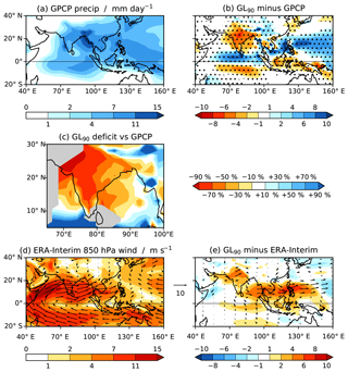
Figure 2 (a) JJAS mean precipitation from GPCP. (b) Bias in JJAS mean precipitation in GL₉₀. Stippling indicates 99 % statistical significance according to a two-tailed t test. (c) Percentage excess (blue) and deficit (red) JJAS mean precipitation in GL₉₀ relative to GPCP. Regions in which the GPCP climatology is below 3 mm day⁻¹ are greyed out. (d) JJAS mean 850 hPa wind (vectors) and wind speed (shading) from ERA-Interim. (e) Bias in JJAS mean 850 hPa wind (vectors; shown only if statistically significant at the 99 % level according to a two-tailed t test) and wind speed (shading; bias of the wind speed, not the magnitude of the bias vectors) in GL₉₀.

These are long-standing biases across many MetUM configurations. For example, in the coupled Hadley Centre Global Environmental Model HadGEM2-AO and in MetUM-GC2 (Williams et al., 2015) the signs of the boreal summer precipitation biases are the same as above. Atmosphere-only experiments with GA3 (Johnson et al., 2016) and GA6 (Walters et al., 2017) show similar biases, although there was no dry bias just south of the Equator in the Indian Ocean and there was a dry bias in the South China Sea.

Over the Indian Ocean GL₉₀ has only small yet statistically significant biases in the mean low-level monsoon flow (Fig. 2d, e), with slightly too-strong southerlies south of the Equator at 75–100^∘ E and a very slightly too-weak jet east of the Horn of Africa. However, it may be that the wind field is quite unrealistic for the given precipitation field. Larger wind biases exist over India, where the flow should be westerly; to the north there is a strong south-westerly bias, with anomalous flow from the Arabian Sea towards the Himalayas, and to the south there is a much weaker but still significant north-westerly bias. Thus, the monsoon flow is bifurcated as it reaches the land, albeit with a much stronger branch to the north than to the south, which is consistent with the dry bias over the country. When the monsoon jet reaches Indochina the strong westerlies erroneously extend into the Pacific Ocean between 5 and 20^∘ N to the extent that they weaken the easterly flow over the tropical Pacific Ocean.

To investigate the effect of regional coupling to the mixed layer ocean we compare GL₉₀ to AO_PO₉₀ (Fig. 3a, c), and to IO₉₀ (Fig. 3b, d; see Table 1). Adding Indian Ocean coupling has very little effect over land, but a substantial impact on biases over ocean (Fig. 3a, c). Indian Ocean coupling reverses the sign of the mean rainfall bias south of the Equator, but increases the wet bias north of the Equator and in the Pacific Ocean. The strong jet extending from the BoB to the west Pacific exists in AO_PO₉₀ and is worsened by Indian Ocean coupling. The effect of Atlantic and Pacific Ocean coupling is similar (Fig. 3b, d) in both precipitation and wind, but with more impact over the Pacific than Indian Ocean. Thus, coupling in any basin significantly degrades the mean state over both the Indian and Pacific Oceans, but most significantly over the basin in which coupling is introduced.

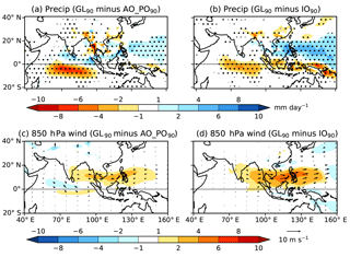
Figure 3 (a, b) JJAS mean precipitation (mm day⁻¹) in GL₉₀ minus that from (a) AO_PO₉₀, (b) IO₉₀. Stippling indicates 99 % statistical significance according to a two-tailed t test. (c, d) Similar but for 850 hPa wind (m s⁻¹), with vectors (shown only if statistically significant at the 99 % level according to a two-tailed t test) and coloured shading as defined in Fig. 2e.

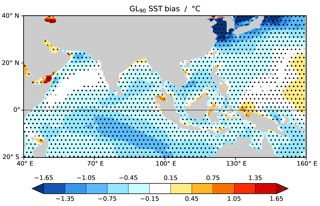
Coupling introduces IAV and ISV in SST, as well as errors in the mean SST. (Although the mean state was constrained through applying corrections to the ocean, there are SST biases of the order of ±0.5 ^∘C in the Indian Ocean; see Fig. 4.) Any or all of these effects could produce the differences seen in Fig. 3. To separate these effects we consider two further experiments: ATM₉₀[$\stackrel{\mathrm{̃}}{\mathrm{GL}}$] with prescribed SST from GL₉₀ with a 31-day smoothing applied to remove much of the SST ISV; and ATM₉₀[$\stackrel{\mathrm{‾}}{\mathrm{GL}}$] with prescribed SST from the mean seasonal cycle taken from GL₉₀ to remove SST IAV and ISV. There are no substantial differences in mean precipitation or 850 hPa wind between GL₉₀ and either of these runs (not shown). Therefore, the change in biases when coupling to the mixed layer ocean is introduced cannot be attributed directly to the introduction of feedbacks at the surface, nor to the ISV or IAV introduced into the ocean. Since SSTs in ATM₉₀[$\stackrel{\mathrm{̃}}{\mathrm{GL}}$] and ATM₉₀[$\stackrel{\mathrm{‾}}{\mathrm{GL}}$] are taken from GL₉₀, the mean state biases are approximately the same in the Indian Ocean in all three experiments. Having eliminated other possibilities, it follows that the change in atmospheric biases when coupling is introduced is attributable to these SST biases.

Figure 4 JJAS SST bias for GL₉₀ relative to SM07. Stippling indicates 99 % statistical significance according to a two-tailed t test. Land and coastally tiled points (i.e. non-zero land fraction) are in grey.

3.2 Intraseasonal variability

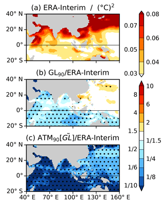
We now investigate ISV using filtered data as described in Sect. 2.3 for GPCP precipitation and ERA-Interim u850 (Fig. 5a, c). In both fields there is significant ISV over the Indian Ocean – both over the Equator and further north in the BoB – as well as over India and the tropical west Pacific. The relative lack of ISV over the Maritime Continent region is consistent with the weak MJO in boreal summer.

Over ocean the ISV of precipitation in GL₉₀ is slightly too high, especially in the west Indian and west Pacific Ocean (Fig. 5b). Notably, however, ISV over the BoB is very similar to observed. The most significant bias is a severe lack of variability (less than a tenth of the observed amount) over the Indian states of Gujarat and Rajasthan, Pakistan, Afghanistan, and the north-east Arabian Sea. The rainfall deficit is over 90 % in the same region (Fig. 2c), suggesting that in the model the monsoon onset does not reach this area or the monsoon is in near-permanent break conditions. u850 in GL₉₀ also exhibits excessive ISV (Fig. 5d; note the different colour scale) over much of the tropical west Pacific, except around the Equator. Although there is a lack of variability over most of the Indian Ocean, especially around the Equator where the northward-propagating events tend to originate, it is not statistically significant. Again there is a lack of variability over India, especially in the west, which in some parts is statistically significant.

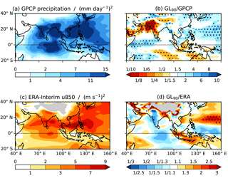
Figure 5 (a) Variance of 24–70-day bandpass-filtered GPCP precipitation for May to October only. (b) Ratio of filtered variance of precipitation from GL₉₀ to that from GPCP. (c, d) As for panels (a, b) but for ERA-Interim u850, with grey shading used to mask out regions where the 850 hPa surface intersects the ground in GL₉₀; stippling indicates 95 % statistical significance according to a two-tailed f test.

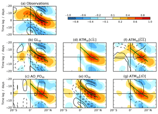
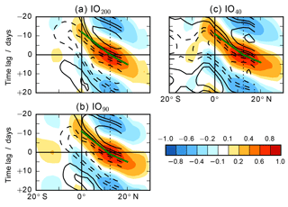
Figure 6 Intraseasonal propagation in the region 70–100^∘ E, 20^∘ S–30^∘ N using 24–70-day bandpass-filtered data, for May to October only, illustrated by lag correlations at each latitude between zonally averaged data and the OLR time series (also filtered) at a base point 85^∘ E, 12.5^∘ N. Coloured shading is for zonally averaged OLR. Green lines show propagation from 0 to 12.5^∘ N and 12.5 to 20^∘ N. Black contours are for zonally averaged SST, with solid (dashed) contours indicating negative (positive) correlation (remembering that negative OLR anomalies correspond to increased convection) and the contour interval being the same as for the coloured shading. SST is shown up to 17.5^∘ N only, where half of the longitude domain is occupied by land. The vertical dotted line shows the latitude of the base point. (a) Observations and reanalysis (AVHRR OLR and ERA-Interim SST), (b) GL₉₀, (c) AO_PO₉₀, (d) ATM₉₀[$\stackrel{\mathrm{̃}}{\mathrm{GL}}$] (note that SST correlations are too small to appear), (e) IO₉₀, (f) ATM₉₀[$\stackrel{\mathrm{‾}}{\mathrm{GL}}$], (g) ATM₉₀[$\stackrel{\mathrm{̃}}{\mathrm{IO}}$].

In Sect. 3.1 (Fig. 3a–c) the changes in the model mean state bias when adding or removing coupling to the mixed layer ocean were attributed to changes in mean SST. A similar conclusion can be drawn in the case of biases in ISV as over ocean there is almost no difference in ISV amplitude between GL₉₀ and ATM₉₀[$\stackrel{\mathrm{̃}}{\mathrm{GL}}$] or ATM₉₀[$\stackrel{\mathrm{‾}}{\mathrm{GL}}$] (not shown).

As mentioned in Sect. 1, the canonical view of summer ISV in the region in question is the northward propagation of convection originating around the equatorial Indian Ocean and propagating northwards over India and the BoB. This propagation is investigated in Fig. 6, which shows lag correlations calculated as described in Sect. 2.3. Lag correlation of OLR is shown in coloured shading. Propagation speed is estimated by joining the points of maximum lag correlation at 0, 12.5, and 20^∘ N with straight line segments. These speeds are listed in Table 2 along with the pattern correlation against observations for each experiment. Lag correlation of SST against OLR at the base point is shown in black contours, with solid contours indicating a negative correlation (i.e. warm SST associated with active convection).

The observations (Fig. 6a) show convection originating just south of the Equator and propagating northwards, reaching 12.5^∘ N about 11 days later before dying out between 20 and 30^∘ N. The propagation doubles in speed from 1.61 to 3.22 m s⁻¹ once it reaches the BoB. There is also a southward branch, also originating from near the Equator and propagating more quickly than its northward counterpart but dying out sooner after about 5 days between 10 and 20^∘ S. The propagation is preceded and followed by a region of opposite-signed OLR anomalies such that the oscillation has a period of around 36 days.

Table 2 Propagation speeds indicated by the green lines in Figs. 6 and 14; pattern correlation between OLR lag correlations in the same figures and for observations (Fig. 6a). Bold text indicates observations.

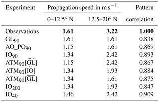
In GL₉₀ (Fig. 6b) propagation is weaker or less coherent than observed, and the origin of the propagating convection lies too far north (on the Equator). The pattern correlation between GL₉₀ and observations is 0.838 (see Table 2); this metric will also be used to compare experiments below. The propagation to 12.5^∘ N is at the correct speed but fails to increase thereafter. The southward branch is present but is considerably weaker and slower than observed. The time lag between opposite phases is approximately 16 days, giving a period of 32 days, which is slightly shorter than observed.

Figure 6a shows that SST and OLR are in quadrature, with positive SST anomalies leading active convection by about 9 days or a quarter-phase. This is consistent with previous observations of both the BSISO and the MJO (Fu and Wang, 2004; Hendon and Glick, 1997; Yang et al., 2008). This phase relationship is simulated well in GL₉₀.

The effect of regional coupling is again investigated in AO_PO₉₀ and IO₉₀ (Fig. 6c, e). In both experiments the northward propagation remains and the pattern correlation with observations is slightly higher than for GL₉₀ (0.869 for AO_PO₉₀ and 0.893 for IO₉₀), suggesting that some aspects of the propagation may be degraded by coupling. However, the difference is minimal and due almost entirely to the lack of southward propagation in the Southern Hemisphere, not to changes in the northward propagation. Indeed, the northward propagation just north of the Equator is considerably stronger with Indian Ocean coupling (GL₉₀ and IO₉₀) than without it. All three experiments considered so far have too slow a phase speed, but IO₉₀ is closest to observations and has an 80 % increase in speed north of 12.5^∘ N.

In both ATM₉₀[$\stackrel{\mathrm{̃}}{\mathrm{GL}}$] and ATM₉₀[$\stackrel{\mathrm{̃}}{\mathrm{IO}}$] the northward propagation remains but is slightly weaker than in their respective coupled experiments, especially between the Equator and about 5–10^∘ N. However, in each case the southward branch of the propagation is (even) weaker than in the coupled experiment. ATM₉₀[$\stackrel{\mathrm{̃}}{\mathrm{GL}}$] has less than 10 % of the SST ISV found in ERA-Interim in the Indian Ocean (Fig. 7c; similarly for ATM₉₀[$\stackrel{\mathrm{̃}}{\mathrm{IO}}$]; not shown). Hence, the ISV in SST provided by coupling is most beneficial to the simulation of ISV of convection in the region of the Equator and is less important northwards of around 10^∘ N. Removing IAV of SST in ATM₉₀[$\stackrel{\mathrm{‾}}{\mathrm{GL}}$] slightly strengthens propagation in the equatorial region, although it does substantially slow propagation north of 12.5^∘ N, which was already too slow in GL₉₀. The impact of SST IAV, which in this model is mostly noise, is a surprising result which we have not been able to explain.

In the experiments with no Indian Ocean coupling (AO_PO₉₀, ATM₉₀[$\stackrel{\mathrm{̃}}{\mathrm{GL}}$], ATM₉₀[$\stackrel{\mathrm{‾}}{\mathrm{GL}}$], and ATM₉₀[$\stackrel{\mathrm{̃}}{\mathrm{IO}}$]) the phase relationship between SST and convection breaks down absolutely. There is no ISV of SST here, yet the convection is able to propagate. This is contrary to Klingaman et al. (2008), who found that HadAM3 produced almost no propagation with monthly mean SST but strong propagation with daily mean SST forcing.

Figure 7 (a) Variance of 24–70-day bandpass-filtered ERA-Interim SST for May to October only. Ratio to ERA-Interim of (b) GL₉₀, (c) ATM₉₀[$\stackrel{\mathrm{̃}}{\mathrm{GL}}$]; stippling indicates 95 % statistical significance according to a two-tailed f test.

3.3 BSISO indices

The MV-EOFs of OLR and u850 used for the BSISO indices were computed using the method of Lee et al. (2013) (see Sect. 2.3) from GL₉₀ and are shown in Fig. 8e–h. These were also computed from observed OLR and reanalysis u850 (Fig. 8a–d). For consistency with earlier figures, we take the wind from ERA-Interim. The meridional component of the 850 hPa wind was computed by regression onto the respective PCs to show a full wind field. The leading two GL₉₀ EOFs have a broadly similar structure at the large scale to those in observations although they explain a smaller fraction of the variance (7.8 % and 4.7 %, respectively, for GL₉₀ compared with 8.4 % and 5.4 % for observations). However, while EOF3 from GL₉₀ has a broadly similar structure to observed EOF4, EOF4 from GL₉₀ does not resemble any of the leading four observed EOFs. Therefore, to use the model EOFs to define a simulated BSISO2 would be inconsistent with the observed intraseasonal oscillation.

The same analysis was performed with the other model experiments described here (not shown). As in GL₉₀, some EOFs broadly match the observations but not always in the correct order, while others do not resemble any of the leading four observed EOFs. Furthermore, the EOFs are not consistent between experiments. Therefore, in the following we project model output onto the EOFs calculated by Lee et al. (2013), which used the NCEP Department of Energy (DOE) Reanalysis II for the wind but are otherwise the same as Fig. 8a–d.

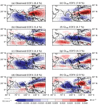
Figure 8 (a–d) MV-EOFs of OLR and u850 calculated from AVHRR OLR and ERA-Interim u850 using the method of Lee et al. (2013) (see their Fig.  2a, b and 3a, b). The meridional component of the wind plotted here was computed by regression onto the respective principal components. Figures in parentheses indicate the percentage of variance explained. (e–f) MV-EOFs calculated by the same method from GL₉₀.

Figure 9 shows the mean annual cycle of variance for each of the leading four pseudo-PCs from observations–ERA-Interim and GL₉₀. (These are pseudo-PCs because the data being projected are not the same used to generate the EOFs; they are hereafter referred to as PCs for brevity.) In observations the variance of PCs 1 and 2 has a broad peak throughout boreal summer (May onwards), tailing off gradually from October onwards. In GL₉₀ they decrease rapidly during August to a minimum in September before increasing again slightly to a secondary maximum in October. Otherwise, the annual cycle is very similar to observations. The annual cycle of PC3 also shows a broad peak in boreal summer in GL₉₀ and is roughly similar to the cycle of PC4 in observations, which is consistent with GL₉₀ EOF3 resembling observed EOF4. In observations PC3 has most of its variance in the pre-monsoon and monsoon onset period but this is not seen in the remaining GL₉₀ PCs. Similar behaviour is seen in other experiments (not shown), suggesting that BSISO1 is simulated reasonably well in MetUM-GOML2.0 (except during September when it is less active) but that the model does not associate BSISO2 with the correct part of the monsoon cycle.

Composites of daily mean precipitation and 850 hPa wind are shown in Fig. 10 as anomalies from climatology using May–October data only. Days are included in the composite only if the BSISO1 amplitude $\sqrt{\mathrm{PC}{\mathrm{1}}^{\mathrm{2}}+\mathrm{PC}{\mathrm{2}}^{\mathrm{2}}}$ is at least 1.5. Both show the same broad structure (as they must by construction, since the OLR and u850 must project reasonably strongly onto the MV-EOFs for a day to contribute to the composite). However, there is a substantial difference over India, where the precipitation anomaly is almost always near zero in the model, especially in the west. We have already seen (Fig. 2b, c) that there is very little rainfall over this area, so there could never be a substantial negative anomaly here (since precipitation is positive definite), but we now see that there is also no significant positive anomaly at any point in the intraseasonal cycle. Indeed, the only region in which the BSISO1 pattern breaks down in the model is over India and, in some phases, the Indian Ocean (e.g. phase 8). The relationship between convection and circulation is fairly realistic, even over India and the Arabian Sea, despite the convective anomalies being weak. Lag correlations (Fig. 11) show that the wind lags the precipitation by 6–10 days (observations) or 2–5 days (GL₉₀). Thus, on intraseasonal timescales, the circulation may respond to convection but not the other way round.

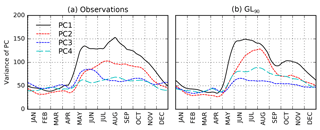
Figure 9 The 30-day smoothed annual cycle of the variance of the leading four pseudo principal components for (a) AVHRR OLR and ERA-Interim u850, (b) GL₉₀. Note that year-round data have been used for the projections, even though the EOFs were computed from boreal summer data only; compare to Lee et al. (2013), Fig. 4.

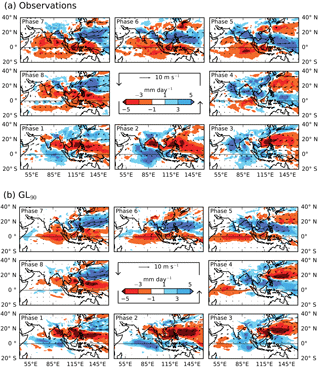
Figure 10 MJJASO anomalies in each BSISO1 phase of precipitation (shading) and 850 hPa wind (vectors; anomalies with amplitude greater than 0.5 m s⁻¹ only) for (a) observations, (b) GL₉₀. Phase 1 is in the bottom left corner and phases continue anticlockwise round the diagram.

To investigate propagation within BSISO1, instances of propagation from one phase to the next (e.g. 4 to 5 or 8 to 1) were found in the time series of phases, with the phase having been replaced with a 0 on days when the BSISO1 amplitude was below 1.5 (i.e. was inside the centre circle in Fig. 12a; PC1 and PC2 were normalized to unit variance). Such propagation events were then classified by their length. For example, a propagation event through phases 6, 7, 8, and 1 has length 4, and BSISO1 may have stayed in each of the given phases for multiple days, provided there were no days breaking the sequence. In 30 years of observations from 1981 to 2010 there were 36 events of length 3 or more (1.2 yr⁻¹), with the longest spanning 6 phases. (In comparison, for the MJO it is not uncommon to have events of length 10 or more; Peatman et al., 2015.) In all experiments the frequency of such events was 1.0–1.3 yr⁻¹, except ATM₉₀[$\stackrel{\mathrm{̃}}{\mathrm{GL}}$], which had only 0.8 yr⁻¹. Simulated events were most likely to be initiated in phase 5, which agrees with observations. Thus, BSISO1 propagation is broadly realistic, with little substantial difference between the experiments.

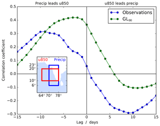
Figure 11 Lag correlation of precipitation and u850 averaged over the boxes shown (inset) for boreal summer (June to September) from observations (GPCP precipitation and ERA-Interim wind, 1997–2010) and GL₉₀.

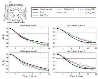
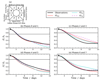
Figure 12 (a) BSISO1 phase diagram showing the eight numbered phases defined by Lee et al. (2013) and with labels indicating the regions of active convection in each. (b–e) Amplitudes A of 15-day composites of BSISO1 events starting in either of the stated phases divided by the amplitude on the first day A₁. An event is defined as beginning on a day when the amplitude $\sqrt{\mathrm{PC}{\mathrm{1}}^{\mathrm{2}}+\mathrm{PC}{\mathrm{2}}^{\mathrm{2}}}\ge \mathrm{1.5}$ (i.e. not inside the centre circle in panel a). The horizontal lines indicate A=1.5 for observations.

Composites of BSISO1 propagation events were computed by selecting all days on which the BSISO1 amplitude exceeded 1.5. These days were all defined as the start of an event and binned according to the BSISO1 phase on that date, with phases paired together: phases 8 and 1, phases 2 and 3, phases 4 and 5, and phases 6 and 7. Composites were calculated by averaging over 15-day time series of the PCs, beginning on each of the selected days, separately for each pair of start phases. The amplitude was then calculated for each day, and the resulting time series are plotted in Fig. 12b–e as a fraction A∕A₁ of the amplitude on the first day. This indicates how rapidly the BSISO1 events decay. The horizontal line on each panel is 1.5∕A₁ for observations, showing the point at which the observed composite decays into the centre circle.

Observed BSISO1 events decay quite rapidly, generally reaching A=1.5 in 3–4 days. Generally speaking, the model composites beginning in phases 4–5 (when active convection is over India and the Maritime Continent) decay too rapidly, and those beginning in phases 2–3 (active over the Indian Ocean and east Asia) and 6–7 (active over the BoB and South China Sea) decay too slowly. GL₉₀ is reasonably realistic in its propagation as the curves shown are closest to the observations, the major exception being for events beginning in phases 6 and 7. As found in Fig. 6, however, there is little consistency between the other experiments as to which performed more realistically. Hence, when BSISO1 becomes strong, the statistics of subsequent propagation are fairly realistic and not systematically dependent on SST biases and variability.

It is notable that there is a fairly realistic representation of the BSISO in MetUM-GOML2.0, even though the model's mean state precipitation is particularly poor. Therefore, a model's ability to simulate boreal summer ISV, and in particular the northward propagation of convection, clearly does not depend on the mean state precipitation.

3.4 Effect of resolution

We now consider the effect of horizontal resolution on the simulation of the ISM in MetUM-GOML2.0 in simulations with Indian Ocean coupling (IO₂₀₀, IO₉₀, and IO₄₀). We first consider the effect on the mean state and then the effect on ISV, including the BSISO1 indices.

GL₉₀ and IO₉₀ have almost exactly the same pattern in the sign of rainfall and 850 hPa wind biases but with some differences in magnitude (Fig. 3b, d). Increasing the resolution from IO₂₀₀ to IO₉₀ (Fig. 13b) slightly improves the mean state precipitation over India and the Indian Ocean (mainly in the Northern Hemisphere). Indian rainfall increases by up to 2 mm day⁻¹, although this is much smaller in magnitude than the dry bias of up to 6 mm day⁻¹ in IO₉₀. Similarly, just north of the Equator in the Indian Ocean there is a wet bias in IO₉₀ of over 10 mm day⁻¹ at its peak, which is at most 4 mm day⁻¹ drier than in IO₂₀₀. Over the BoB the increase in precipitation from IO₂₀₀ to IO₉₀ is roughly half the magnitude of the dry bias in IO₂₀₀ (not shown). The greatest change resulting from this increase in resolution, however, is in the Pacific Ocean, where there is no coupling. There is a substantial decrease in precipitation and weakening of the westerly jet extending over the same region, approximately halving the magnitude of the IO₂₀₀ biases. As the resolution increases from IO₉₀ to IO₄₀ (Fig. 13c) the changes in mean precipitation are generally insignificant, with some minimal decreases in the bias over ocean and almost no change over land.

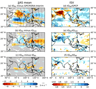
Figure 13 (a–c) JJAS mean precipitation (shading; mm day⁻¹) and 850 hPa wind (vectors; m s⁻¹; values below 1 m s⁻¹ not shown): (a) IO₉₀ minus GPCP–ERA-Interim, (b) IO₉₀ minus IO₂₀₀, (c) IO₄₀ minus IO₉₀. Grey shading indicates that precipitation is statistically insignificant at the 99 % level according to a two-tailed t test; vectors (black) are shown only if statistically significant at the 99 % level according to a two-tailed t test. (d–f) Ratio of MJJASO variance of 24–70-day bandpass-filtered precipitation in (mm day⁻¹)²: (d) IO₉₀ over GPCP observations, (e) IO₉₀ over IO₂₀₀, (f) IO₄₀ over IO₉₀. Stippling indicates 99 % statistical significance according to a two-tailed t test.

The changes in the precipitation bias with increasing resolution found here are consistent over ocean with those found by Johnson et al. (2016) in MetUM-GA3. However, the latter study did not find improvement in the bias over India when moving from 200 km grid spacing to 90 km which we see here for MetUM-GOML2.0, suggesting this may be linked to air–sea coupling or the change from GA3 to GA6.

At 90 km grid spacing there is very little difference in ISV of precipitation when all ocean basins are coupled (GL₉₀; Fig. 5b) and when only the Indian Ocean is coupled (IO₉₀; Fig. 13d). In the region where the most significant bias exists – over north-west India, Pakistan, and the north Arabian Sea where there is less than a tenth of the observed variance – IO₉₀ is still a significant improvement over IO₂₀₀ (Fig. 13e), especially over the Arabian Sea. In IO₄₀ (Fig. 13f) there is almost no significant change in variance, except for an increase over the Arabian Sea at the entrance to the Persian Gulf. Over the land areas affected by the significant lack of variance in IO₉₀, variance slightly increases with resolution. As with the change in mean state, variance over India improves as resolution increases, but with a much greater change from 200 to 90 km (2-fold or more over all of India) than from 90 to 40 km (the change being negligible over most of the country).

We now consider the effect on the northward intraseasonal propagation of OLR (Fig. 14). Increasing resolution from 200 km through 90 to 40 km slightly increases the pattern correlation against observations and gives increasingly realistic propagation speeds, albeit always slower than observed (Table 2). At 0–12.5^∘ N the speed is 1.34 m s⁻¹ (IO₂₀₀ and IO₉₀) and 1.46 m s⁻¹ (IO₄₀, while the observed speed is 1.61 m s⁻¹), and at 12.5–20^∘ N it is 1.93 m s⁻¹ (IO₂₀₀) and 2.42 m s⁻¹ (IO₉₀ and IO₄₀), while the observed speed is 3.22 m s⁻¹). The phase relationship between OLR and SST is correct at all three resolutions in Fig. 14. The southward branch of propagation is not distinct in IO₂₀₀ and IO₉₀; it is present in IO₄₀ but is substantially too slow.

Figure 14 As Fig. 6 but for (a) IO₂₀₀, (b) IO₉₀ (repeat of Fig. 6e, for reference), (c) IO₄₀.

Figure 15 As Fig. 12 but for IO₂₀₀, IO₉₀, and IO₄₀.

The amplitudes of BSISO1 phase composites are shown for the three Indian Ocean coupling experiments in Fig. 15. The rates of decay of propagation events are similar to those seen earlier in Fig. 12, with events starting in phases 2 and 3 tending to decay too slowly and those starting in phases 4 and 5 tending to decay too quickly (except IO₄₀). However, none of the resolutions consistently outperforms the others, so the longevity of propagation events is not systematically improved by using any particular grid box size.

4 Discussion and conclusions

This study has evaluated the simulation of the ISM in MetUM-GOML2.0, which uses a mixed layer ocean (with vertical mixing but no advection) coupled to the MetUM atmosphere, with atmosphere and ocean at the same resolution. We have investigated the effects of regional air–sea coupling (by switching off the mixed layer ocean in certain regions and imposing SST there) and horizontal resolution. Through a flux correction technique we are able to investigate each of these in a framework in which the ocean mean state is constrained to observations, so differences in SST biases are minimized between experiments, allowing us to investigate changes to model configuration without the complication of knock-on effects from a changing basic state.

Table 3 List of further experiments referred to in Sect. 4. See Table 1 for full explanation.

All experiments contain biases in JJAS precipitation and 850 hPa wind. For example, there is a severe dry bias over India (with a rainfall deficit of over 70 % in much of the country) and the Maritime Continent and a wet bias over the north Indian Ocean and the tropical Pacific. Similar biases have been seen in other MetUM experiments (Johnson et al., 2016) and in the National Centers for Environmental Prediction Climate Forecast System model version 2 (Bombardi et al., 2015; Goswami et al., 2014).

Coupling in the Indian Ocean (shown by the difference between GL₉₀ and AO_PO₉₀) or the Pacific and Atlantic Ocean (GL₉₀ and IO₉₀) degrades the atmospheric JJAS mean state over the sea, in particular over the west tropical Pacific and the Indian Ocean. By comparing with atmosphere-only experiments forced with the GL₉₀ SST but with either ISV or IAV removed, it was shown that basic state degradations are due to small SST biases introduced with coupling (Sect. 3.1).

Further experiments (see Table 3 for details) which were not presented in Sect. 3 for brevity confirm these conclusions. For example, AO_PO₉₀[$\stackrel{\mathrm{‾}}{\mathrm{GL}}$] has no coupling in the Indian Ocean, but has the same mean SST as GL₉₀ there. Therefore, the only difference between AO_PO₉₀[$\stackrel{\mathrm{‾}}{\mathrm{GL}}$] and AO_PO₉₀ is the mean Indian Ocean SST. The JJAS mean precipitation difference between AO_PO₉₀[$\stackrel{\mathrm{‾}}{\mathrm{GL}}$] and AO_PO₉₀ (not shown) is almost identical to the difference between GL₉₀ and AO_PO₉₀ (Fig. 3a). Thus, the effect of introducing coupling in the Indian Ocean (the latter comparison) is very similar to the effect of just introducing SST biases in the same region (the former comparison), further supporting the conclusion that the change in mean state due to coupling is attributable to the introduction of SST biases.

Similar conclusions can be drawn for the Pacific. The effect of Pacific Ocean coupling is indicated by comparing IO₉₀ with IO_PO₉₀. The wet bias over the Pacific Ocean exists in IO₉₀ but is considerably worse in IO_PO₉₀; the Maritime Continent dry bias, which is mostly absent in IO₉₀, is substantial in IO_PO₉₀, and the strong westerly jet which erroneously extends over the north tropical Pacific is much stronger in IO_PO₉₀. These all suggest that coupling degrades the local basic state in the Pacific just as in the Indian Ocean. Furthermore, the mean states in ATM₉₀[$\stackrel{\mathrm{‾}}{\mathrm{GL}}$] and AO_PO₉₀[$\stackrel{\mathrm{‾}}{\mathrm{GL}}$], which have the same SST in the Indian Ocean and very similar SST biases in the Pacific and Atlantic, are almost the same, consistent with differences in atmospheric mean state depending on differences in SST mean state only. Similarly, in ATM₉₀[$\stackrel{\mathrm{̃}}{\mathrm{IO}}$] and ATM₉₀[$\stackrel{\mathrm{̃}}{\mathrm{GL}}$], in which the SSTs are similar in the Indian Ocean but differ in the Pacific and Atlantic, the only substantial mean state differences in the atmospheric mean state are outside the Indian Ocean.

The coupled SST biases responsible for the degradation of the atmospheric mean state are a limitation of this model, as they have been minimized by the ocean flux correction technique yet are non-zero (Sect. 2.1). The reason why these biases remain is not fully understood. One possibility is due to errors in the mean wind stress. For example, in Fig. 2e the wind speed is too strong in GL₉₀ in the southern tropical Indian Ocean, which could explain the cold bias there (Fig. 4) due to excessive wind-driven mixing or evaporative cooling. This cold bias is not easily removed. The 15-day relaxation timescale used in the correction technique was chosen by Hirons et al. (2015) after experimentation with a range of values; even a 1-day timescale was not enough to remove SST biases as heat added to the ocean to correct the cold bias is quickly mixed down by the strong surface winds.

Consistent with the severe dry bias over India in MetUM-GOML2.0, there is also a significant lack of ISV over the same region. The 24–70-day bandpass-filtered variance is very low (e.g. for precipitation GL₉₀ has less than 10 % of the observed variance over west India; Fig. 5a), and the BSISO, while exhibiting reasonably realistic propagation in terms of progression from one BSISO1 phase to the next (Sect. 3.3), has almost no associated precipitation anomalies over most of India (Fig. 10b). Thus, although the active-break cycle is simulated over most of south-east Asia, the Indian monsoon is in near-permanent break conditions in the model. However, the modelled ISV in the BoB is very close to that in GPCP precipitation and ERA-Interim u850. Thus, MetUM-GOML2.0 is more realistic in this sense than NCEP CFSv2 (which is coupled with a full dynamical ocean), in which there is excessive ISV in the BoB as well as in the east Arabian Sea and east equatorial Indian Ocean (Goswami et al., 2014).

The oscillation consists of the northward propagation of convection over the Indian Ocean, BoB, and India, as well as shorter-lived southward propagation over the Indian Ocean in the Southern Hemisphere. The propagation was investigated using lag correlation propagation diagrams (Fig. 6). The lag correlations of OLR change slightly between experiments but there is no significant overall impact of local coupling, as shown by the fact that the pattern correlations with observations vary little by experiment (Table 2). The largest differences tend to be found in the southward branch of the propagation and in the northward branch up to around 5^∘ N. In these regions, having coupling – in particular in the Indian Ocean – is beneficial, with stronger and more coherent simulated propagation. This improvement with coupling is consistent with DeMott et al. (2011, 2014) (in the Community Climate System Model, CCSM, and Community Atmosphere Model, CAM) and Fu and Wang (2004) (in ECHAM4).

We note that in MetUM-GOML2.0 coupling acts to degrade the basic state but generally to improve ISV and propagation. Other studies have shown changes in ISV, especially the MJO, in conjunction with changes in mean state, but a poorer mean state is not always associated with improved ISV as here. In atmosphere-only configurations of the MetUM, increasing the rate of mixing entrainment and detrainment for deep- and mid-level convection affects the tropical mean state precipitation (Bush et al., 2015; using GA3), in particular producing more rainfall over the north-west tropical Pacific Ocean and less over the equatorial Indian Ocean and Maritime Continent. These increases in entrainment and detrainment rates also improve MJO forecast skill (Klingaman and Woolnough, 2014a; using GA2). Furthermore, Inness et al. (2003) improved the strength of MJO propagation through the Maritime Continent by reducing biases in SST and wind in the coupled Hadley Centre MetUM (HadCM3) through flux adjustments.

Studies with other models have also shown relationships between changes in mean state and ISV. Kim et al. (2011) performed 10 experiments with five atmosphere-only GCMs and discovered a systematic difference in boreal summer mean state precipitation between those experiments with strong ISV and weak ISV, with stronger ISV being associated with excess rainfall over the south Asian and north-west Pacific monsoon regions. Studies with ECHAM4 have shown that the simulated MJO is sensitive to the choice of prescribed SST (Liess and Bengtsson, 2004), with an experiment by Liess et al. (2004) showing an improved MJO when the AGCM is forced with SSTs from a coupled version of the model rather than observed SST. Sperber (2004) found biases in SST and wind to degrade MJO propagation in CCSM2.

In the present study, SST IAV (when coupling is switched on; compare to GL₉₀ and ATM₉₀[$\stackrel{\mathrm{‾}}{\mathrm{GL}}$]) affects the intraseasonal propagation (Fig. 6b, f), although it does not impact the mean state (not shown). The interannual standard deviation of JJAS SST in GL₉₀ is of the order of 0.25^∘C in the tropical Indian Ocean. A question which remains unanswered is why the SST IAV should have an effect on the ISV of convection.

The effect of resolution was investigated by comparing experiments with only the Indian Ocean coupled at three resolutions (Sect. 3.4). The mean state precipitation improves somewhat when changing from 200 to 90 km grid spacing, but there is little change when increasing resolution again to 40 km (Fig. 13a–c). A similar result was found by Ogata et al. (2017) when increasing resolution in both the MetUM GA3 and the Meteorological Research Institute of Japan atmosphere-only model (MRI-AGCM3.2), with precipitation increasing over India, the Maritime Continent and the Indian Ocean just south of the Equator and decreasing over the tropical Pacific and the Indian Ocean just north of the Equator. GL₉₀ also shows an improved mean state over GL₂₀₀ (not shown) but the difference over the Pacific Ocean is smaller than for IO₂₀₀ and IO₉₀. Thus, resolution has less of an impact when there is local coupling than when the SST is prescribed. Increasing resolution also improves intraseasonal propagation and the BSISO, but only to a minor extent. Ogata et al. (2017) showed that in MRI-AGCM3.2 the intraseasonal propagation also strengthens with increasing resolution, although they found that the ISV in MetUM GA3 weakened. However, they used an atmosphere-only model with a different MetUM configuration from the present study (GA3 rather than GA6).

This study has shown that although there is an impact from including local air–sea interactions on simulating the processes responsible in the ISM using a mixed layer ocean, these impacts are not always beneficial, with an overall worsening of the mean state biases due to SST biases. However, there are slight improvements to the simulation of the active-break cycle and BSISO.