the Creative Commons Attribution 4.0 License.
the Creative Commons Attribution 4.0 License.
 | 26 Sep 2018
An ensemble of AMIP simulations with prescribed land surface temperatures
Duncan Ackerley
Robin Chadwick
Dietmar Dommenget
Paola Petrelli
General circulation models (GCMs) are routinely run under Atmospheric Modelling Intercomparison Project (AMIP) conditions with prescribed sea surface temperatures (SSTs) and sea ice concentrations (SICs) from observations. These AMIP simulations are often used to evaluate the role of the land and/or atmosphere in causing the development of systematic errors in such GCMs. Extensions to the original AMIP experiment have also been developed to evaluate the response of the global climate to increased SSTs (prescribed) and carbon dioxide (CO2) as part of the Cloud Feedback Model Intercomparison Project (CFMIP). None of these international modelling initiatives has undertaken a set of experiments where the land conditions are also prescribed, which is the focus of the work presented in this paper. Experiments are performed initially with freely varying land conditions (surface temperature, and soil temperature and moisture) under five different configurations (AMIP, AMIP with uniform 4 K added to SSTs, AMIP SST with quadrupled CO2, AMIP SST and quadrupled CO2 without the plant stomata response, and increasing the solar constant by 3.3 %). Then, the land surface temperatures from the free land experiments are used to perform a set of “AMIP prescribed land” (PL) simulations, which are evaluated against their free land counterparts. The PL simulations agree well with the free land experiments, which indicates that the land surface is prescribed in a way that is consistent with the original free land configuration. Further experiments are also performed with different combinations of SSTs, CO2 concentrations, solar constant and land conditions. For example, SST and land conditions are used from the AMIP simulation with quadrupled CO2 in order to simulate the atmospheric response to increased CO2 concentrations without the surface temperature changing. The results of all these experiments have been made publicly available for further analysis. The main aims of this paper are to provide a description of the method used and an initial validation of these AMIP prescribed land experiments.
- Article
(12181 KB) - Full-text XML
-
Supplement
(4680 KB) - BibTeX
- EndNote


The works published in this journal are distributed under
the Creative Commons Attribution 4.0 License. This license does not affect
the Crown copyright work, which is reusable under the Open Government
Licence (OGL). The Creative Commons Attribution 4.0 License and the OGL are
interoperable and do not conflict with, reduce or limit each
other.
© Crown copyright 2018
In order to evaluate the atmosphere and land modules of general circulation models (GCMs), simulations can be run under Atmospheric Model Intercomparison Project (AMIP) specifications (Gates, 1992; Gates et al., 1999). Typically, both sea surface temperatures (SSTs) and sea ice concentrations (SICs) are prescribed from observations over some reference period (e.g. 1979–2014 in the Coupled Model Intercomparison Project phase 6 – CMIP6 – experiment; see Eyring et al., 2016) with the atmosphere and land allowed to respond freely to the SST and SIC field. Such AMIP simulations help to understand the role of the atmosphere and/or land in the development of model errors. In addition to the standard AMIP experiments, quadrupled CO2 (amip4xCO2) and spatially uniform 4 K SST increase (amip4K) experiments were incorporated as part of CMIP5 (see Taylor et al., 2012) by the Cloud Feedback Model Intercomparison Project (CFMIP; Bony et al., 2011). The amip4xCO2 experiment was designed to identify the rapid cloud response to increased CO2 and the amip4K experiment was intended to investigate the impact of the dynamical response of the atmosphere (to the higher SST) on cloud feedbacks (Bony et al., 2011). The CFMIP experiments have also been used to examine the regional precipitation response to both CO2 forcing and higher SSTs (e.g. Bony et al., 2013; Chadwick et al., 2014; He and Soden, 2015). The amip4xCO2 and amip4K experiments are also included in CMIP6 (see Webb et al., 2017). While the AMIP experiments described above are designed to investigate the response of the land and the atmosphere to the imposed SST and CO2 conditions, there is scope to further isolate the response of the atmosphere by prescribing the land conditions too. Such a method of prescribing the land has not been attempted (to our knowledge) as part of the CFMIP/CMIP initiative; however, there are several key issues from the CFMIP and CMIP6 experiments that could at least be partially addressed by running a set of AMIP simulations with prescribed land conditions, for example:
-
How does the Earth system respond to forcing and what is the role of the land in that response? (adapted from Eyring et al., 2016)
-
How can the understanding of circulation and regional-scale precipitation (particularly over the land) be improved? (adapted from Webb et al., 2017)
Prescribing global surface temperatures (including the land) in order to, for example, suppress the surface response to a radiative forcing is not a new idea. Such an approach has previously been used to understand the strength of coupling between the land and atmosphere in GCMs (Koster et al., 2002). In another example, Shine et al. (2003) prescribed land temperatures in order to estimate the climate sensitivity parameter of an intermediate complexity GCM in a variety of greenhouse gas and aerosol forcing experiments. Furthermore, a better estimate of the radiative forcing from, e.g. quadrupling CO2 may be attained from GCMs by fixing land surface temperatures as the changes in land temperature can change the atmosphere (e.g. circulation, clouds and precipitation) in a manner that can affect the simulated global radiation balance (Andrews et al., 2012a, 2015). Unfortunately, the method of prescribing land temperatures (as well as SSTs) has not been developed widely for use in multinational modelling efforts (such as CMIP) and has only been used in one-off idealised modelling experiments such as those described by Dommenget (2009) and Ackerley and Dommenget (2016).
Work by Bayr and Dommenget (2013) used the prescribed land temperature experiments from Dommenget (2009) and data from the CMIP3 experiment to show that higher land temperatures (and specifically increasing the land–sea thermal contrast) are an important driver of circulation change under global warming. However, there are many different mechanisms/forcing agents that can cause the land surface temperatures to increase (or decrease), which may also have an impact on the global circulation. For example, land surface temperatures increase by more than 4 K in amip4k-type experiments (e.g. Joshi et al., 2008), which indicates that land temperatures can change substantially in response to changes in SSTs. Land temperatures also increase directly in response to increased CO2 concentrations, which cause increased downwelling long-wave radiation and cloud adjustments (Dong et al., 2009; Cao et al., 2012; Becker and Stevens, 2014). This increase in land temperatures forms part of the direct CO2 effect, which drives both global (Allen and Ingram, 2002) and regional (Bony et al., 2013; Chadwick et al., 2014; Merlis, 2015; He and Soden, 2015) precipitation responses; however, it is currently unclear how much of this effect is due to increases in atmosphere or land temperatures. To complicate matters further over the land, the degree of land surface warming and precipitation change are also sensitive to the physiological response of plant stomata, which close as CO2 concentrations increase and thereby reduce evapotranspiration and precipitation locally (Doutriaux-Boucher et al., 2009; Boucher et al., 2009; Andrews et al., 2011). Finally, land surface temperatures (and therefore circulation and precipitation) also respond to changes in insolation (e.g. the “abrupt solar-fixed SST” experiments in Chadwick et al., 2014; Andrews et al., 2012b). Given that all of the different forcing agents outlined above have very different impacts on land temperatures and the global circulation (and precipitation), it would be useful to quantify the separate contributions of the land (temperature and soil moisture), the atmosphere (e.g. increased long-wave absorption), plant physiology and SSTs to the circulation change separately (and any other aspects of regional and global climate change). Prescribed land experiments could achieve this, and the modelling framework developed by Ackerley and Dommenget (2016) for the Australian Community Climate and Earth System Simulator (ACCESS) provides an opportunity to do so. There is also scope to provide a platform to share the results with the wider scientific community through the Australian National Computing Infrastructure (NCI) and the ARC Centre of Excellence for Climate System Science (ARCCSS).
The main aim of this study is to describe and validate a set of AMIP simulations run with freely varying land conditions against those with prescribed land conditions and observational datasets. This study also presents an evaluation of further experiments that employ different combinations of land conditions with the different SST, CO2 and insolation specifications. Finally (and most importantly), the study provides information on where these data can be accessed for others to use.
The model used, experimental outline and reference datasets are given in Sect. 2, including a description of how the land datasets were generated. In Sect. 3, the AMIP simulations with prescribed land are then validated against the original AMIP (freely varying land) simulations from which the land conditions were taken. The results of the AMIP simulations with different combinations of land conditions, SSTs, CO2 concentrations and the solar constant are described in Sect. 4.1. The results of uniformly increasing the land surface temperatures alone by 4 K and of raising both the land surface and sea surface temperatures by 4 K are discussed in Sect. 4.2. The summary, concluding remarks and future work (e.g. further development opportunities) are given in Sect. 5.
2.1 Model
2.1.1 General background
The GCM used in this study is the Australian Community Climate and Earth System Simulator (primarily ACCESS1.0) in an atmosphere-only configuration, which is identical to that used in Ackerley and Dommenget (2016). The version of ACCESS1.0 used here has a horizontal grid spacing of 3.75∘ (longitude) × 2.5∘ (latitude) and 38 vertical levels. Parameterised processes include precipitation, cloud, convection, radiative transfer, boundary layer processes and aerosols. The representation of the land surface and soil processes is of primary relevance to this study, which is simulated by the Met Office Surface Exchange Scheme (MOSES; Cox et al., 1999; Essery et al., 2001). Subgrid-scale surface heterogeneity is represented by splitting the grid box into smaller “tiles” of which there are nine different types specified. Tiles may be vegetated (e.g. grasses) or non-vegetated (e.g. bare soil) and the tiles within a grid box can comprise any fractional combination of the surface types. Surface variables (such as temperature, long-wave and short-wave radiation, and latent and sensible heat fluxes) are calculated for each tile individually and then summed to give a representative grid box mean value, which is passed back into the main model. Also of relevance is the representation of soil properties (i.e. soil moisture and temperature), which is simulated over four vertical layers (0.1, 0.25, 0.65 and 2 m deep). The model code is available by following the instructions in the code and data availability section.
2.1.2 Prescribing land temperatures
The land surface temperatures are prescribed using the same method described in Ackerley and Dommenget (2016) – the reader is directed there for more in-depth discussion. Nevertheless, the calculation of the surface temperature in the free land simulations (i.e. land surface temperature and soil moisture and temperature are allowed to vary freely) and the code changes made to prescribe it are discussed here. An initial estimate of the land surface temperature is calculated from the existing surface conditions using
where the temperature of the first soil layer from the previous time step is denoted as Ts (K), A* is the coefficient for converting fluxes into temperature in this instance (W m−2 K−1), Rs is the net radiation into the surface (both long-wave and short-wave, W m−2), H is the surface sensible heat flux (W m−2), λE is the latent heat flux (W m−2), Cc is the areal heat capacity of the surface (J m−2 K−1), Δt is the length of the time step (s), and is the surface temperature from the time step before the current time (K). The value of T* from Eq. (1) is then adjusted implicitly within the model depending upon the moisture availability and changes of state such that
A land surface temperature increment due to evaporation (Eq. 2 – , K) is calculated from the adjustments to the sensible heat flux (ΔH, W m−2) and the latent heat flux (Δ(λE), W m−2) that are made after diagnosing the moisture availability. The temperature increment is then simply added to the value of T* calculated in Eq. (1) (i.e. , K) via Eq. (3). If there is no snow present, then T* is unchanged for the rest of the time step at that land point. If, however, snow is present on the land surface, then the temperature is adjusted further to account for any snowmelt (, K) and is again simply added to the value calculated in Eq. (3) by the following:
More details on these equations (i.e. Eqs. 1–4) can be found in the relevant papers that describe the MOSES module (i.e. Essery et al., 2001; Cox et al., 1999).
When the surface temperatures are prescribed, Eq. (1) is simply changed to be
where TPRES is the input, prescribed temperature (K) field (discussed in Sect. 2.2.2, below). Furthermore, the increments calculated in Eqs. (2)–(4) are set to zero so that the surface temperature cannot change implicitly within the time step. The surface radiation budget therefore only depends upon TPRES.
It is also worth noting here that the existing ACCESS model code has the option for prescribing deep soil temperatures and soil moisture content. When the soil temperatures and moisture are prescribed (as stated in the experiments below), that option is switched on in the code and soil moisture and deep soil temperatures are set from an input field as outlined in the experiments below.
2.2 AMIP simulations
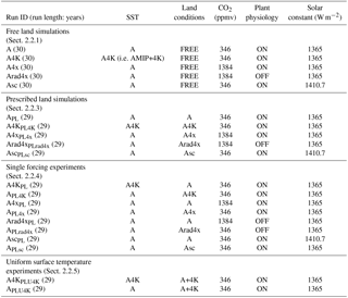
All experiments undertaken in this study are summarised in Table 1 for ease of reference. More details on these simulations are given in Sect. 2.2.1, 2.2.3, 2.2.4 and 2.2.5 below.
Table 1A summary of the experimental specifications. In the sea surface temperature (SST) column, A refers to SSTs from the AMIP run and A4K to those of the AMIP+4K (A4K) run. FREE refers to freely varying land temperatures and soil moisture. Plant physiology is set to ON when vegetation responds to CO2 changes and OFF when it uses the default value (346 ppmv); i.e. only atmospheric radiation responds to higher CO2. Experiments are ordered following the descriptions in Sect. 2.2.1, 2.2.3, 2.2.4 and 2.2.5.
2.2.1 Free land simulations
The following simulations are undertaken with freely varying land conditions (“land conditions” refers to surface temperature, soil temperature and soil moisture from here on); i.e. Eqs. (1)–(4) are used by the model.
- (1)
The AMIP run uses prescribed, observational SSTs and sea ice concentrations from 1979 to 2008 (30 years long). CO2 concentrations are set to 346 ppmv, and sulfur dioxide, soot and biomass burning aerosol emissions are representative of those for the year 2000 C.E. Land conditions are allowed to vary freely. The experiment is denoted as A from here on.
- (2)
The AMIP4K run is the same as A but a uniform 4 K is added to the SST field (denoted as A4K from here on).
- (3)
The AMIP4xCO2 run is the same as A but CO2 is quadrupled to 1384 ppmv (denoted as A4x from here on).
- (4)
The AMIP4xCO2 no plant physiological response run, i.e. radiative (rad) only, is the same as A4x but the plant physiological response to CO2 is switched off (as described in Andrews et al., 2011; Boucher et al., 2009; Doutriaux-Boucher et al., 2009, and is denoted as Arad4x from here on). This is done by setting the CO2 concentration used in the photosynthesis calculation in the vegetation scheme to 346 ppmv but allowing the radiation scheme to “see” the quadrupled value (i.e. 1384 ppmv).
- (5)
The AMIP +3.3 % solar constant run is the same as A except the solar constant is increased by ∼3.3 % to 1410.7 W m−2, as done by Andrews et al. (2012b), which gives a similar-sized radiative forcing to the 4xCO2 experiments (denoted as Asc from here on).
All AMIP simulations were initialised with conditions from 1 October 1978 and run until the end of December 2008.
2.2.2 Specifications for generating the prescribed land conditions
In order to generate the necessary fields to prescribe the land conditions, instantaneous values of the surface temperature on each tile, and soil temperature and moisture (on each soil level) are output every 3 h from experiments (1)–(5) above. In the prescribed land simulations, the land conditions are read in by the model every 3 h and updated (by interpolation) every hour (two time steps). Furthermore, land conditions from the first 15 months of the AMIP free land simulations are not used (i.e. the prescribed land simulations are run from January 1980 to December 2008, inclusive) to ensure that no impacts from the land scheme “spinning up” are included in the prescribed runs. The surface temperature, soil moisture and soil temperatures are all prescribed every 3 h for the whole period (1980–2008) to minimise the differences between free and prescribed land simulations. The interpolated, 3-hourly data are used instead of time step (30 min) data due to limitations of reading in such large datasets in the current ACCESS1.0 framework. The prescribed land condition experiments will therefore not be identical to the free land simulations. Nevertheless, Ackerley and Dommenget (2016) note that a simulation with temperatures updated each time step is “almost climatologically indistinguishable” from another using 3-hourly data. Therefore, corresponding free and prescribed land simulations should be climatologically alike, which is evaluated in Sect. 3. Finally, land surface temperatures are not prescribed over both the permanent ice sheets (Antarctica and Greenland, to avoid the development of negative temperature biases that are discussed in Ackerley and Dommenget, 2016) and within/on sea ice. The impact of not specifying the temperatures over the ice sheets or sea ice temperature is likely to be negligible and is discussed in Sect. 3. The input data fields are available by following the instructions in the code and data availability section.
2.2.3 AMIP prescribed land simulations
All simulations that have prescribed land conditions are denoted with a PL. The AMIP prescribed land simulations use Eq. (5) instead of Eq. (1), both and set to zero, and the following boundary conditions are used:
- (6)
The AMIP prescribed land run is the same as A except land conditions are also prescribed from A. Experiment is denoted as APL from now on.
- (7)
The AMIP4K prescribed land run is the same as A4K except land conditions are prescribed using the output from A4K. Experiment denoted as A4KPL4K from now on.
- (8)
The AMIP4xCO2 prescribed land run is the same as A4x except land conditions are prescribed using the output from A4x. The experiment is denoted as A4xPL4x from now on.
- (9)
The AMIP4xCO2 no plant physiological response prescribed land run is the same as Arad4x except land conditions are prescribed using the output from Arad4x. The experiment is denoted as Arad4xPLrad4x from now on.
- (10)
The AMIP +3.3 % solar constant prescribed land run is the same as Asc except land conditions are prescribed using the output from Asc. The experiment is denoted as AscPLsc from now on.
2.2.4 Combinations of AMIP land and ocean conditions (“combined” experiments)
In these experiments, different combinations of land, SST, atmospheric CO2 and solar irradiance boundary conditions are used. These experiments were designed to single out the impact of the land response to a forcing on the atmosphere or the impact of that forcing agent without the land responding. Again (as in Sect. 2.2.3), Eq. (5) instead of Eq. (1), and both and are set to zero for these simulations. The boundary conditions used in these experiments are as follows:
- (11)
SST field from A4K and land conditions from A; from now, denoted as A4KPL;
- (12)
SST field from A and land conditions from A4K; from now, denoted as APL4K;
- (13)
SST and land conditions from A with CO2 concentrations the same as in A4x; from now, denoted as A4xPL;
- (14)
SST and CO2 concentrations the same as A and land conditions from A4x; from now, denoted as APL4x;
- (15)
CO2 concentrations (no plant response) from Arad4x and SST and land conditions from A; from now, denoted as Arad4xPL;
- (16)
SST and CO2 concentrations the same as A and land conditions from Arad4x; from now, denoted as APLrad4x;
- (17)
SST and land conditions from A and solar constant as in Asc; from now, denoted as AscPL; and
- (18)
Land conditions from Asc and SST and solar constant as in A; from now, denoted as APLsc.
2.2.5 Uniform surface temperature perturbation (“uniform” experiments)
An extra two experiments are undertaken to identify the impact of applying a uniform increase in temperature over the land only (analogous to the AMIP4K SST experiment but for the land) and a uniform global increase in surface temperature (i.e. global warming with minimal land–sea contrast). As in Sect. 2.2.3 and 2.2.4, Eq. (5) is used instead of Eq. (1), and both and set to zero for these simulations. The boundary conditions used in these experiments are as follows:
- (19)
uniform increase in land surface temperatures from A by 4 K and SST field from A4K; from now, denoted as A4KPLU4K; and
- (20)
uniform increase in land surface temperatures from A by 4 K and SST field from A; from now, denoted as APLU4K.
In both experiments (19) and (20), soil temperatures and moisture are prescribed from the A experiment.
2.3 Reference datasets
ERA-Interim (ERAI) data are taken from 1980 to 2008 (Dee et al., 2011) for both the surface air temperature (TAS) and pressure at mean sea level (PSL) for comparison with the A and APL simulations. ERAI reanalysis data have been used to evaluate TAS globally for the fifth Coupled Model Intercomparison Project (Flato et al., 2013). ERAI data provide a globally complete (unlike surface observations which are heterogeneously spread), observationally constrained (as is PSL) dataset for comparison with the simulations in this study. Furthermore, there is good agreement between reanalysis-derived TAS and gridded data from station-based estimates (Simmons et al., 2010), which suggests the ERAI-derived TAS is a reliable dataset.
For precipitation, the Climate Prediction Centre Merged Analysis of Precipitation (CPC CMAP; Xie and Arkin, 1997; Arkin et al., 2018) data, for the years 1980–2008 inclusive, are used. The CMAP data are derived from a combination of satellite-based instruments. It is important to note that, while there are biases in any reference dataset and others could be used (e.g. GPCP or CMORPH for rainfall, see Adler et al., 2003; Joyce et al., 2004, respectively), the focus of the paper is not to explore the model biases themselves. The reference datasets are simply used to show that there is no negative impact on the simulated climate (relative to the free land simulations) when the land conditions are prescribed.
3.1 Surface air temperature: TAS
The difference (A minus ERAI) in grid-point mean (averaged over all simulated years) TAS is plotted in Fig. 1. Positive anomalies (∼0.5 K) are visible over many ocean basins but the largest differences are over the land (>1 K magnitude over north Africa, Antarctica and the Himalaya). Nevertheless, the temperature biases in Fig. 1a are consistent with those presented in Flato et al. (2013) from the CMIP5 multi-model mean (their Fig. 9.2b), and the global mean root mean square difference (RMSD) of 1.68 K (Table 2) is also comparable to the mean absolute grid-point errors of 1–3 K also given in Flato et al. (2013) (their Fig. 9.2c). The largest model errors primarily occur in the regions that have the largest uncertainties in the ERAI TAS dataset (e.g. north Africa, Antarctica and the Himalaya; Flato et al., 2013, their Fig. 9.2d). Finally, the pattern correlation between A and ERAI fields is approximately 1 (Table 2), which indicates that relatively low and high surface temperatures are simulated in the correct geographical locations. Overall, therefore, the TAS field in the ACCESS1.0 AMIP simulation (and the biases) is consistent with those of other models.
The difference in TAS for APL relative to A is plotted in Fig. 1b. It is immediately obvious that the differences in TAS1 between APL and A are much smaller than those between A and ERAI (Fig. 1a). There are also very few places where the differences are statistically significant in Fig. 1b, and the largest changes are at high latitudes where sea ice is located (sea ice temperatures are not prescribed). Furthermore, the RMSD is much larger between A and ERAI than between APL and A (1.69 and 0.13 K, respectively, in Table 2). Overall, in terms of TAS, the A and APL simulations are climatologically very similar such that the intermodel differences are much smaller than the model–reanalysis differences.
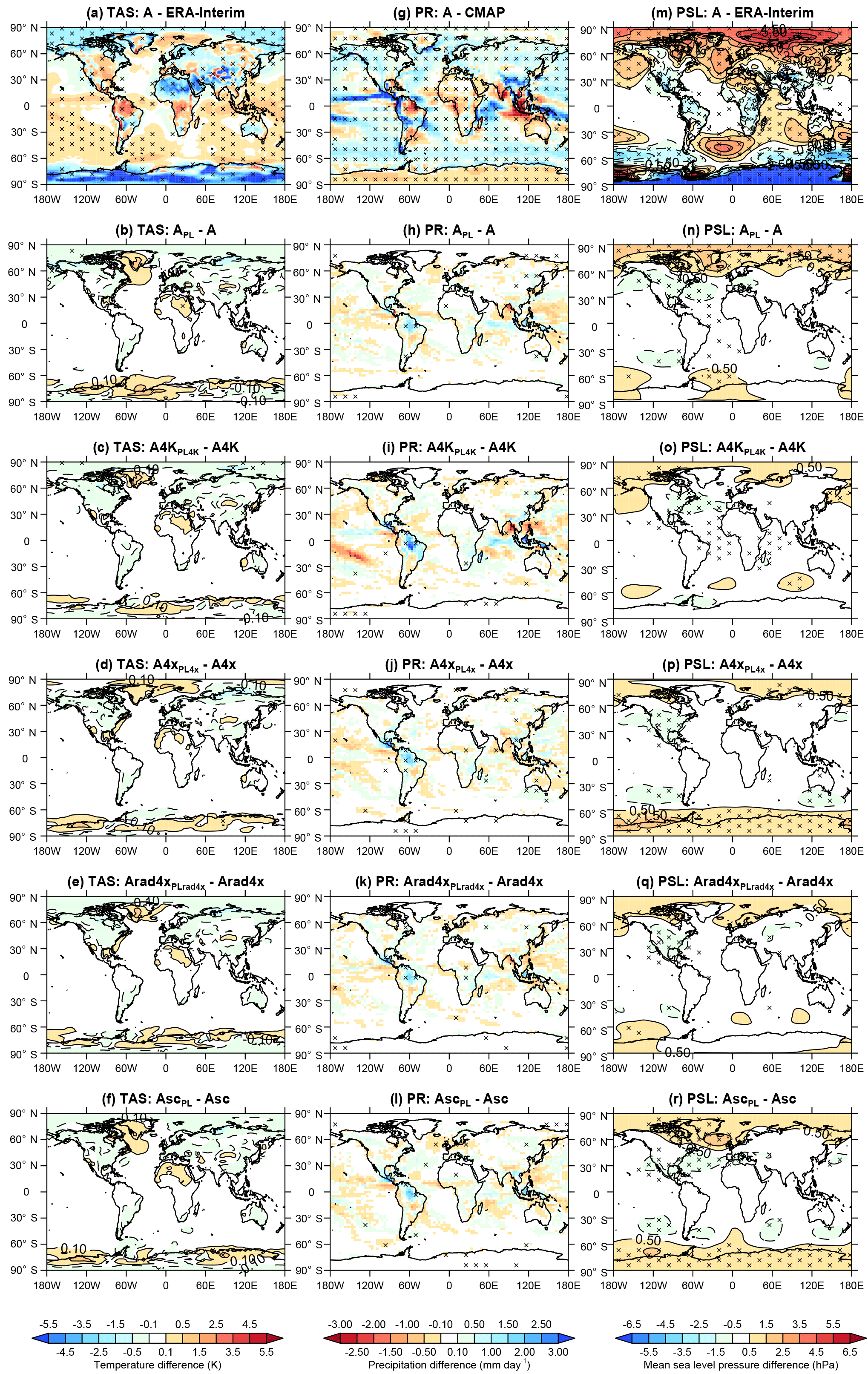
Figure 1Differences in surface air temperature (TAS, K) for (a) A minus ERAI, (b) APL minus A, (c) A4KPL4K minus A4K, (d) A4xPL4x minus A4x, (e) Arad4xPLrad4x minus Arad4x, and (f) AscPLsc minus Asc. Equivalent differences between observations/simulations are given in panels (g–l) and (m–r) for precipitation (PR, mm day−1, CMAP data used in panel g) and mean sea level pressure (PSL, hPa, ERAI data used in panel m), respectively. The points labelled with an “x” indicate the differences are statistically significant using Student's t test (p≤0.05).
Each of the prescribed land (PL) simulations (A4KPL4K, A4xPL4x, Arad4xPLrad4x and AscPLsc, described in Sect. 2.2.3) is compared with their corresponding free land simulations (A4K, A4x, Arad4x and Asc, respectively; Sect. 2.2.1) in order to validate them. The differences in TAS are non-significant over the vast majority of the globe for the prescribed vs. free land simulations (Fig. 1c–f). Moreover, the RMSD between each experiment pair is 0.11 K with pattern correlations of unity or close to unity (see Table 2). Therefore, the values of TAS in the A4KPL4K, A4xPL4x, Arad4xPLrad4x and AscPLsc runs are almost climatologically indistinguishable from those of A4K, A4x, Arad4x and Asc, respectively (as intended).
In order to further validate whether the PL simulations adequately reproduce the climate of their free land counterparts under different boundary conditions (i.e. SST+4K, 4xCO2 and +3.3 % insolation), the differences in TAS between corresponding free and prescribed land pairs, e.g. (A4KPL4K minus APL) minus (A4K minus A), are plotted in Fig. 2a–d. Furthermore, the RMSD and pattern correlations for the differences in TAS between those corresponding prescribed and free land pairs are given in Table 3. Pattern correlations are proximately 1 for all experiment pairs (Table 3). Furthermore, the RMSD values are <0.1 K, which is a similar magnitude to the differences plotted in Fig. 1c–f and smaller than the differences in TAS associated with each change in boundary condition (see Figs. S1a–d and S2a–d in the Supplement). Therefore, the changes in TAS for A4KPL4K, A4xPL4x, Arad4xPLrad4x and AscPLsc relative to APL are almost identical to those of A4K, A4x, Arad4x and Asc relative to A (compare Figs. S1a–d and S2a–d). Overall, the responses of TAS to the perturbed SST, CO2 and insolation in the prescribed land simulations are very similar to those in the free land simulations.
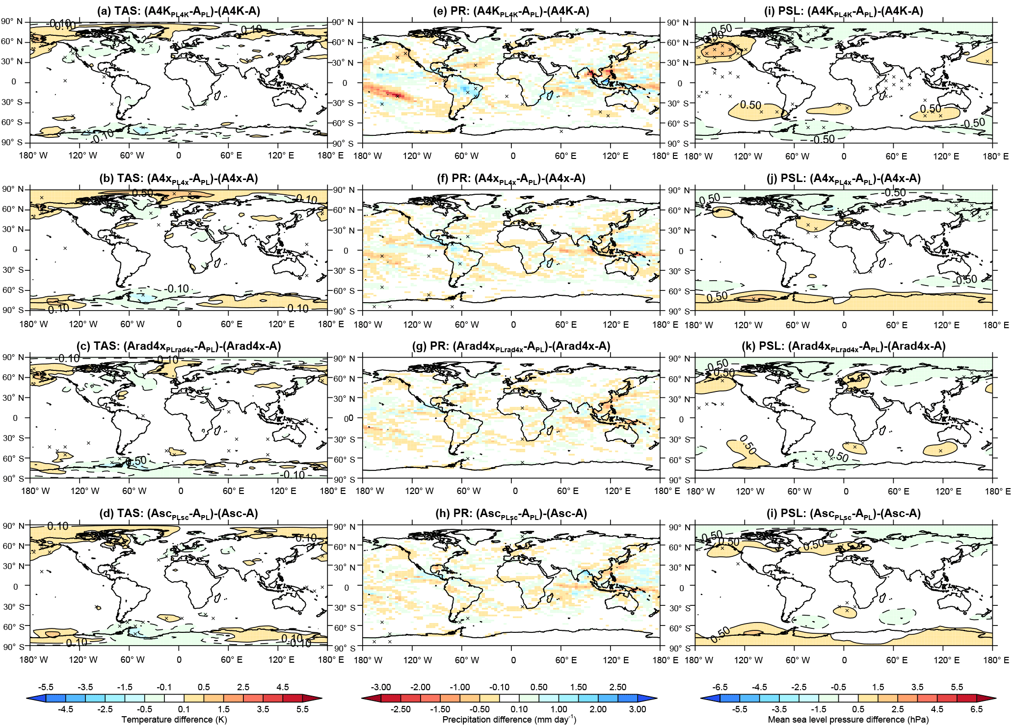
Figure 2Differences in surface air temperature (TAS, K) for (a) (A4KPL4K minus APL) minus (A4K minus A), (b) (A4xPL4x minus APL) minus (A4x minus A), (c) (Arad4xPLrad4x minus APL) minus (Arad4x minus A), and (d) (AscPLsc minus APL) minus (Asc minus A). Equivalent differences between simulations are given in panels (e–h) and (i–l) for precipitation (PR, mm day−1) and mean sea level pressure (PSL, hPa), respectively. The points labelled with an “x” indicate the differences are statistically significant using Student's t test (p≤0.05).
3.2 Precipitation: PR
Differences between the A simulation and CMAP precipitation fields are plotted in Fig. 1g. Precipitation is too high over the western Indian Ocean, the northern tropical Pacific and within the midlatitudes of both hemispheres. Conversely, precipitation is too low over the south-western Maritime Continent, central Africa, Amazonia and over the Antarctic. The precipitation biases over the western Indian Ocean and Amazonia are also visible in the CMIP5 multi-model mean (see Fig. 9.4b in Flato et al., 2013). The rainfall biases in the remaining regions (listed above) are consistent with those presented in Walters et al. (2011) for HadGEM2-A (the model from which ACCESS1.0 is derived; see Bi et al., 2013). The RMSD is 1.25 mm day−1 (Table 2) for A relative to CMAP, which is consistent with the values presented for HadGEM2-A by Walters et al. (2011) (2.02 mm day−1 for JJA and 1.54 mm day−1 for DJF, relative to GPCP data). Overall, the precipitation biases in the A simulation are consistent with those in other GCMs.
The differences in precipitation between APL and A are plotted in Fig. 1h, and (as with TAS) it is clear that almost none of the differences in precipitation are significant. Furthermore, the RMSD between APL and CMAP is almost identical to that of A relative to CMAP, and the RMSD for APL relative to A is smaller by almost a factor of 5 (see Table 2) than relative to CMAP. The pattern correlations between APL and A are also approximately equal to 1, which shows that regions with relatively high and low precipitation (climatologically) are almost identical in the two respective simulations. Therefore, the differences in PR between APL and A are small in terms of the climatological mean.
As with TAS, the differences in PR between other prescribed land simulations (A4K, A4x, Arad4x and Asc) and their respective free land runs (4KPL4K, A4xPL4x, Arad4xPLrad4x and AscPLsc) are plotted in Fig. 1i–l. Very few of the differences in PR are statistically significant; however, there is an increase in precipitation over Amazonia in all of the prescribed land runs relative to their free land counterparts. A similar region of higher precipitation over Amazonia between prescribed and free land simulations is also seen in Ackerley and Dommenget (2016). Given that there is no change in surface temperature or soil moisture (both prescribed) it may be that rainwater is accumulating in the vegetation canopy and being re-evaporated (see Cox et al., 1999). Indeed, there is an increase in the latent heat flux over the region with higher precipitation in all of the prescribed land simulations relative to the free land simulations (see Figs. S3 and S4, which show the change in canopy water loading for APL relative to A; see the Supplement). This is a systematic bias in the prescribed land simulations relative to their free land counterparts; however, the precipitation is approximately 1–2 mm day−1 higher in the prescribed land runs, which almost exactly offsets the ∼2 mm day−1 dry bias for the A simulation relative to CMAP (Fig. 1g). Therefore, the prescribed land simulation is closer to the observed estimate than the free land simulation. A more detailed investigation into Amazonian rainfall is beyond the scope of this current general overview and evaluation paper, but such a study may be useful to understand the dry bias over the Amazon in the free land simulations.
As with TAS, the RMSD and pattern correlations for the differences in PR between corresponding prescribed and free land pairs, e.g. (A4KPL4K minus APL) minus (A4K minus A), are given in Table 3. The pattern correlations lie between 0.8 and 0.95 (Table 3) for the change in PR between the perturbed PL simulations (A4KPL4K, A4xPL4x, Arad4xPLrad4x and AscPLsc) and their free land counterparts (A4K, A4x, Arad4x and Asc), relative to their respective control simulations (APL and A). Furthermore, the RMSD values lie in the range 0.22–0.38 mm day−1, which is a similar magnitude to the differences plotted in Figs. 1c–f and 2e–h. Therefore, the differences between corresponding prescribed and free land simulations (e.g. A4KPL4K and A4K) are much smaller than the PR differences caused by the boundary condition changes (see Figs. S1e–h and S2e–h). The lower pattern correlation values and higher RMSDs for PR relative to TAS are likely to be due to TAS being more highly constrained by the prescribed surface temperatures than PR (i.e. TAS is diagnostically calculated from the surface temperature and the temperature of the lowest model level).
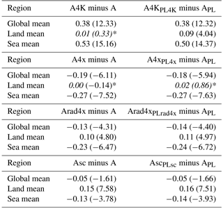
For further verification, the changes in global, ocean and land mean precipitation are presented in Table 4. The differences in precipitation between the free land and PL experiment pairs are all the same sign (i.e. corresponding positive or negative) and lie within ±0.08 mm day−1 (i.e. small). The largest difference occurs over land in A4KPL4K experiment where the increase in precipitation (relative to APL) is statistically significant, whereas for A4K relative to A, it is not. The higher precipitation over the Amazon (Fig. 2e) is likely to be contributing to the higher land mean precipitation in A4KPL4K relative to A4K. Conversely, the dry bias over the Amazon in the free land simulations may equally be a factor for the muted response of the mean precipitation over land in the A4K experiment relative to A4KPL4K. Again, a more detailed investigation into Amazonian rainfall biases is beyond the scope of this study; however, given the sensitivity of this region to model configuration and climate change (see Good et al., 2013), the prescribed land simulation may be a useful tool to investigate Amazon precipitation further. Another point of note is that precipitation increases significantly on land in the runs without plant physiological responses to CO2 but does not change in those with plant physiological responses (Table 4). In the A4x and A4xPL4x experiments, plant stomata respond to increasing CO2 by narrowing and thereby reducing moisture availability for precipitation from transpiration. In Arad4x and Arad4xPLrad4x, however, the stomatal response is switched off and so evapotranspiration can increase in response to land surface warming, as can precipitation. These results are consistent with those of Doutriaux-Boucher et al. (2009), Boucher et al. (2009) and Andrews et al. (2011).
Table 2The area-weighted RMSDs and pattern correlations (PCs) for surface air temperature (TAS), precipitation (PR) and mean sea level pressure (PSL) for the A and APL simulations relative to the observational (OBS) reference datasets (rows 2 and 3). Rows 4–8: the RMSDs and PCs for each prescribed land simulation relative to its counterpart free land simulation (experiment names defined in Sect. 2).
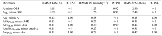
“≈1” implies that the correlation coefficient is not unity but rounds to unity when only two decimal places are considered.
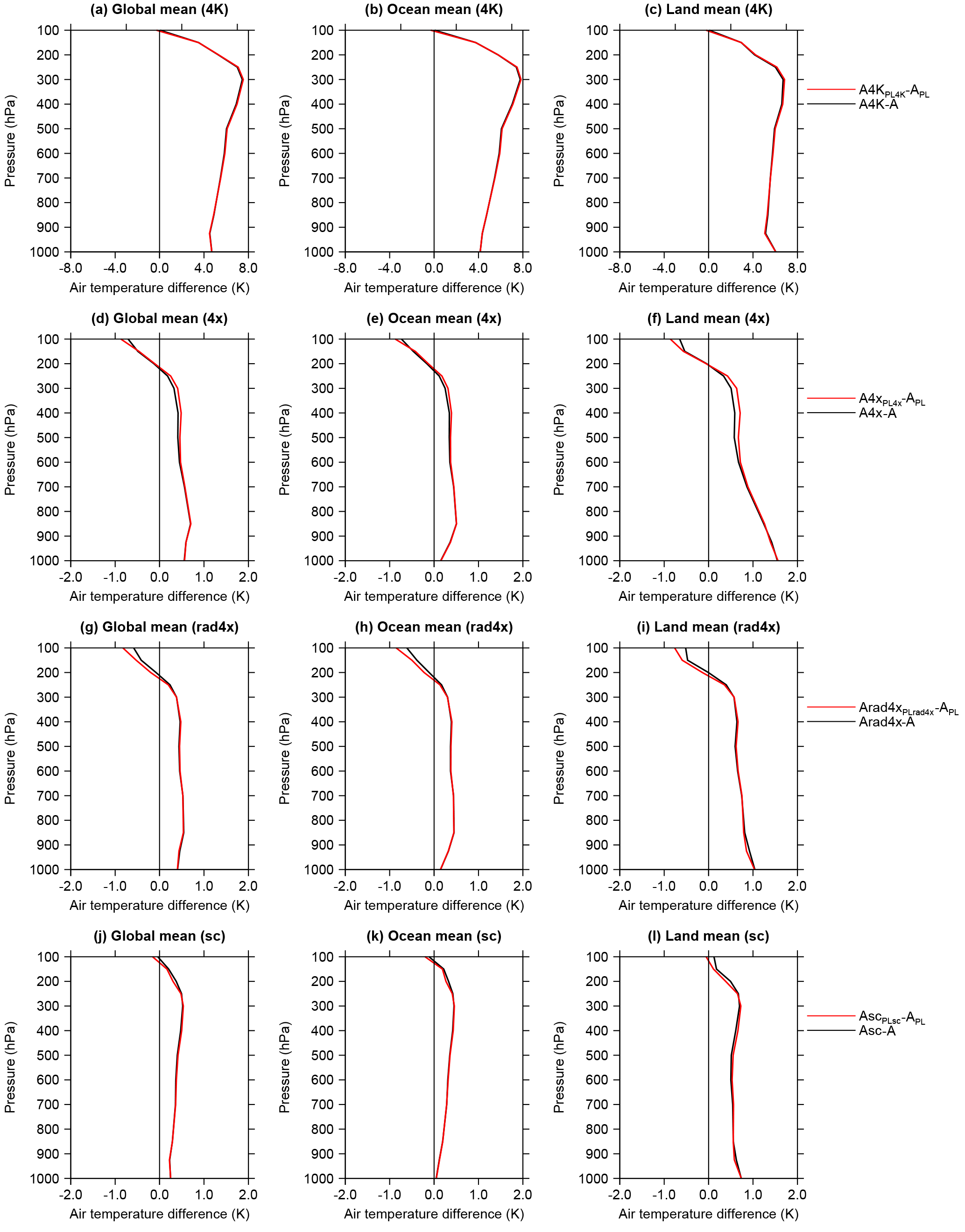
Figure 3Differences (relative to A or APL; see key for each row) in global mean (a, d, g, j), ocean-only mean (b, e, h, k) and land-only mean (c, f, i, l) air temperature (K) for (a–c) the A4K experiments, (d–f) the A4x experiments, (g–i) Arad4x experiments and (j–l) the Asc experiments, respectively.
3.3 Pressure at mean sea level: PSL
The difference in PSL for A relative to ERAI is plotted in Fig. 1m in order to provide a surface-based indication of changes in the atmospheric circulation (as also done in Collins et al., 2013). The RMSD for A relative to ERAI is 2.4 hPa; however, the pattern correlation is almost unity (see Table 2) and indicates that regions with relatively high and low PSL correspond well. There are several biases in the PSL field, nonetheless. Positive PSL anomalies are visible in A relative to ERAI over the Arctic (largest anomaly around 90∘ E), the north Pacific, northern Africa and the Mediterranean, and between 30 and 60∘ S in each ocean basin (see Fig. 1m). There are negative anomalies over central and southern Africa, South America, North America and Antarctica. The PSL anomalies, though, are consistent with those presented in Martin et al. (2006) (their Fig. 6), who used a higher-resolution (half the grid spacing of ACCESS1.0) version of HadGEM2 (from which ACCESS1.0 is developed; see Bi et al., 2013).
Table 3The area-weighted RMSDs and PCs for the response in the climate to the perturbed boundary conditions (SST+4K, 4xCO2 and +3.3 % solar constant; Sect. 2) for each prescribed land pair relative to the corresponding free land pair.
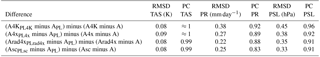
“≈1” implies that the correlation coefficient is not unity but rounds to unity when only two decimal places are considered.
Table 4The difference in global, land point and sea point mean precipitation, mm day−1 (%) for each of the specified simulations in rows 1, 5, 9 and 13 (details of each simulation are given in Sect. 2). Numbers in italics and marked with an asterisk are not statistically significant using Student's t test (p>0.05).
The RMSD (2.48 hPa) and pattern correlations (≈1) for the APL simulation are almost identical to those of A relative to ERAI. Furthermore, the RMSD between APL and A is 0.45 hPa and the pattern correlation is unity (Table 2), which indicates that the PSL field is reproduced well in the APL simulation relative to A. The main difference in the PSL fields between APL and A occurs over the Arctic (Fig. 1n), which is consistent with the lower temperatures there (see Fig. 1b). Nevertheless, over the vast majority of the globe, the differences in the simulated PSL field between APL and A are not statistically significant.
The RMSDs for each of the other corresponding PL and free land simulations (e.g. A4KPL4K vs. A4K) lie between 0.3 and 0.5 hPa with pattern correlations of close to unity (see Table 2). The magnitudes and distribution of PSL in the PL simulations therefore compare well with their free land counterparts (as with APL vs. A). In terms of grid-point PSL values, the largest differences occur in the northern and southern polar regions (see Fig. 1o–r); however, the differences in PSL are not statistically significant over the vast majority of grid points. Overall, the small differences in the PSL fields between the PL and free land simulations suggest that the simulated, climatological global circulations are very similar.
Again (as with TAS and PR), the RMSD and pattern correlations for the differences in PSL between corresponding prescribed and free land pairs, e.g. (A4KPL4K minus APL) minus (A4K minus A), are given in Table 3. The RMSDs between the change in PSL associated with each boundary condition perturbation for the PL simulations relative to their free land counterparts lie between 0.33 and 0.45 hPa (Table 3). The largest RMSD for PSL changes (0.45 hPa) occurs in the SST+4K experiments, i.e. (A4KPL4K minus APL) relative to (A4K minus A); however, the changes in PSL associated with increasing global SSTs are much larger (approximately ±3.5 hPa; see Fig. S2i) than the RMSD. The changes in PSL associated with quadrupling CO2 are ±2.5 hPa (Fig. S2j and k) and are larger than the RMSD between the corresponding prescribed and free land simulations (0.38 and 0.35 hPa; see Table 3). The smallest changes in PSL occur in the increased solar constant simulations (around ±1.5 hPa; Fig. S2l) and likewise, the lowest RMSD between the PL and free land simulations (0.33 hPa; see Table 3). Finally, the pattern correlations between the PL and free land simulations are all >0.9 (column 7, Table 3), which shows that the spatial changes in PSL associated with each boundary condition change are also very similar. The largest grid-point differences in PSL primarily occur in polar regions, where surface temperatures are not prescribed (Fig. 2i–l); however, the differences in PSL are not statistically significant over the majority of the globe.
3.4 Vertical profiles: global, ocean-only and land-only means
As a final validation, the vertical changes in mean air temperature (ta) associated with the SST+4K, 4xCO2, 4xCO2rad and +3.3 % insolation are plotted for the PL (red lines) and free land (black lines) in Fig. 3. Furthermore, the ta profile differences are compared with results from other studies (where available) for further validation of these simulations.
The global, ocean and land mean changes in ta for A4K minus A are almost identical to those of A4KPL4K minus APL (values lie within approximately ±0.1 K; see Fig. 3a–c). Furthermore, ta values are higher at all levels from 1000 to 100 hPa, with the largest increase around 300 hPa. Overall, atmospheric dry stability increases as a result of increasing global SST by 4 K both globally and over the ocean with a slight decrease in dry stability over land between approximately 1000 to 500 hPa. The changes to the ta profiles in both the PL (A4KPL4K minus APL) and free simulations (A4K minus A) agree with those described in Dong et al. (2009) and He and Soden (2015).
The differences in ta between the prescribed (red lines) and free (black lines) land 4xCO2 experiments (both with and without plant physiology) are plotted in Fig. 3d–i. As with the SST+4K experiments, the differences between the prescribed and free land simulations are small ( K) and primarily restricted to the land in the A4xPL4x and A4x experiments. The largest changes in ta from quadrupling atmospheric CO2 occur around 850 hPa for the global and ocean mean regardless of whether the plant physiological response to CO2 is included or not (Fig. 3d, e, g and h) in agreement with Dong et al. (2009), Kamae and Wanatabe (2013), Richardson et al. (2016) and Tian et al. (2017).
Finally, the ta profiles for the 3.3 % increase in insolation simulations (Asc and AscPLsc relative to A and APL, respectively) are plotted in Fig. 3j–l. Again, the differences between the free and prescribed land simulations are small ( K) and the vertical distributions of ta changes are almost identical. Atmospheric dry stability increases globally and over the ocean, with the largest increases in ta around 300 hPa (Fig. 3j and k), which compares well with the model results of Cao et al. (2012). Conversely, air temperatures increase uniformly by approximately 0.8 K from 950 to 500 hPa in both the Asc and AscPLsc simulations (Fig. 3l) over the land; however, dry static stability increases around 300 hPa (again in agreement with Cao et al., 2012).
Overall, the differences in ta between the prescribed and free land simulations are small relative to the changes associated with each boundary condition change. Furthermore, the changes in ta in both the prescribed and free land simulations are consistent with those in other studies.
Only the changes in surface air temperature are discussed below for each of the combined and uniform temperature perturbation experiments (outlined in Sect. 2.2.4 and 2.2.5, respectively) to verify that the temperature response is consistent with the imposed boundary conditions. The changes in precipitation and circulation associated with these experiments are to be discussed in a future piece of work (Chadwick et al., 2018).
4.1 Combined experiments
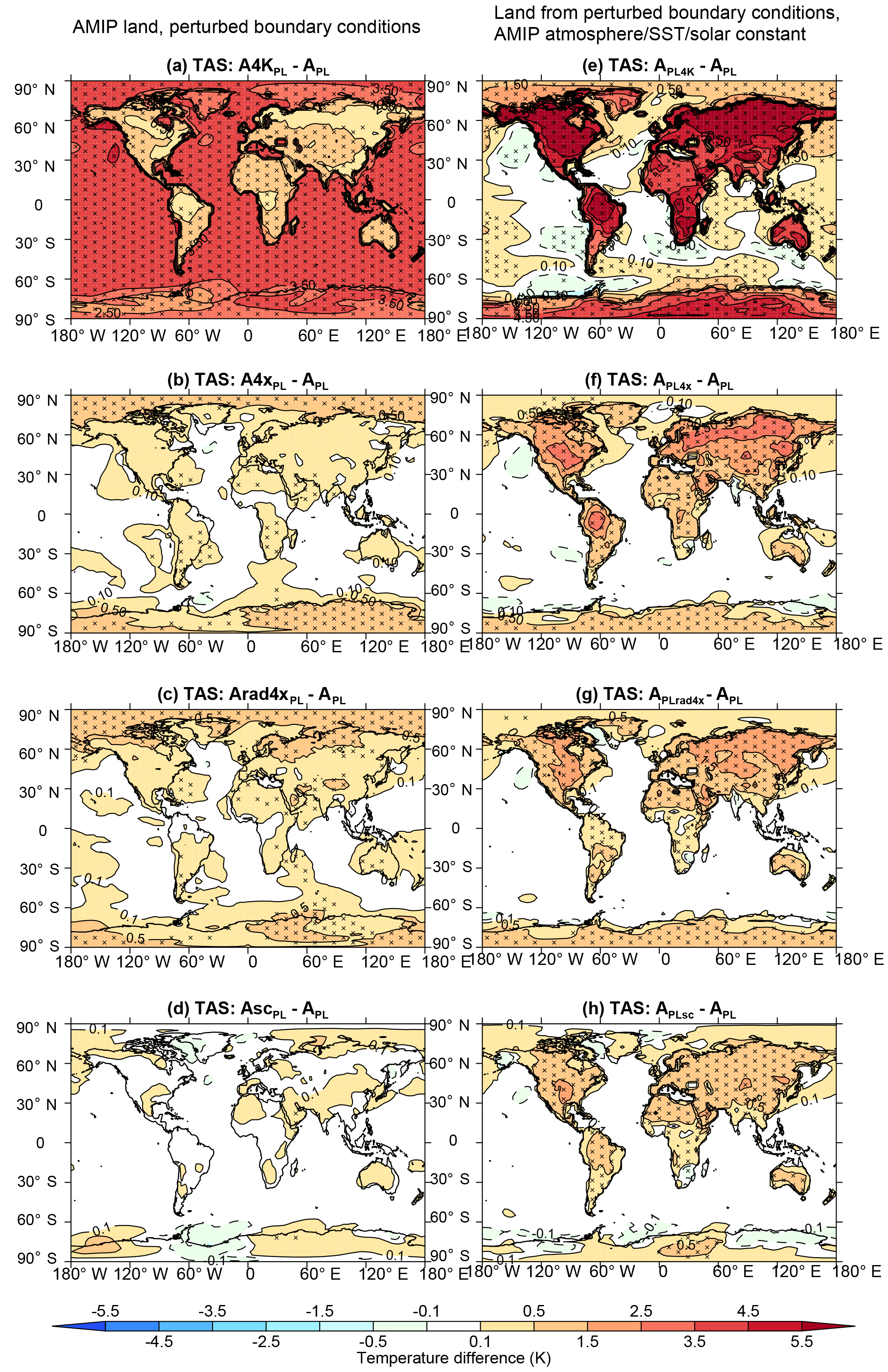
Figure 4Differences in surface air temperature (TAS, K) for (a) A4KPL minus APL, (b) A4xPL minus APL, (c) Arad4xPL minus APL, (d) AscPL minus APL, (e) APL4K minus APL, (f) APL4x minus APL, (g) APLrad4x minus APL, and (h) APLsc minus APL. The points labelled with an “x” indicate the differences are statistically significant using Student's t test (p≤0.05)
Changes in TAS over the land can be seen in the experiments that use land conditions from the AMIP runs with changed boundary conditions, i.e. A4KPL, A4xPL, Arad4xPL and AscPL (Fig. 4a–d). As the calculation of TAS is performed by interpolating between the surface temperature and that of the lowest model level in ACCESS1.0, changes in the temperature at level 1 will change TAS even if surface temperatures are unchanged. This explains why TAS increases over the land in A4KPL, as the global atmosphere will warm from increased SST (Fig. 4a). There are also positive TAS anomalies over high latitudes in all the experiments plotted in Fig. 4 relative to APL, which is unsurprising as the snow cover and surface temperatures are not prescribed there. The changes in TAS are also higher over the ocean than the land (land–sea contrast is 0.252).
The changes in TAS for A4xPL, Arad4xPL and AscPL are not statistically significant over the majority of the land surface and may be related to adjustments in the surface sensible and latent heat fluxes as the atmosphere responds to the increase in CO2 concentrations or insolation (Fig. 4b–d). Conversely, the changes in TAS over the land are statistically significant and positive in all runs with perturbed land surface conditions (Fig. 4e–h). Overall, relative to APL, the changes in TAS for the simulations described in Sect. 2.2.4 (plotted in Fig. 4) are consistent with the land surface and boundary condition perturbations imparted upon them.
4.2 Uniform experiments
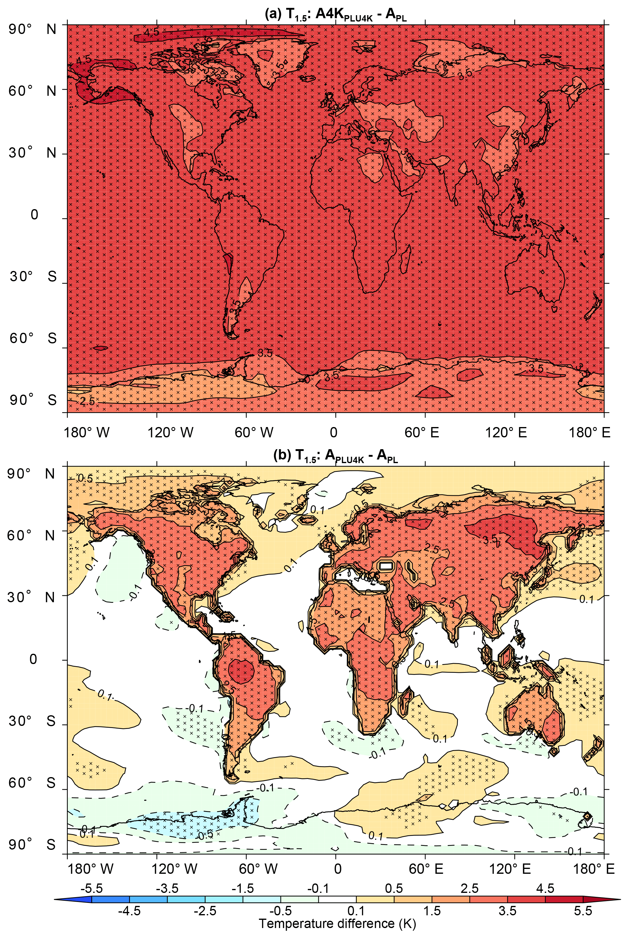
Figure 5Differences in surface air temperature (TAS, K) for (a) A4KPLU4K minus APL and (b) APLU4K minus APL. The points labelled with an “x” indicate the differences are statistically significant using Student's t test (p≤0.05).
The spatial differences in TAS are plotted in Fig. 5a for the A4KPLU4K simulation relative to APL. The changes in TAS over the land and the sea are very similar with a land–sea thermal contrast of 0.9. The main difference in TAS between the land and the ocean is over Antarctica and Greenland where the surface temperatures are not prescribed and the temperature change is muted.
In the APLU4K experiment (relative to APL), TAS increases over all land points by 1.5–4.5 K (statistically significant) except over Antarctica and Greenland where temperatures are not prescribed (Fig. 5b). Another interesting feature of this simulation is that the land–sea thermal contrast is very large (with a value of 40); however, the large contrast is unsurprising given the large temperature increase is only applied to the land.
This paper has outlined the results of a novel set of AMIP-type model simulations that use prescribed SSTs and land surface fields (surface temperature, soil temperature and soil moisture). The main results of this study are as follows:
-
The differences in climate between the simulations with freely varying land conditions and their prescribed land counterparts (e.g. A vs. APL) are much smaller than the underlying systematic errors relative to the observational datasets (i.e. A vs. OBS). Therefore, prescribing the land conditions does not degrade the model-simulated climate.
-
The changes in global mean precipitation and vertical temperature profiles in the A4K, A4x, Arad4x and Asc experiments are almost identical to those of their corresponding prescribed land simulations – A4KPL4K, A4xPL4x, Arad4xPLrad4x and AscPLsc.
-
The changes in TAS associated with holding the land fixed while changing a forcing agent (e.g. A4xPL) or fixing the forcing agent and using the land response to that agent (e.g. APL4x) are consistent with imposed state and are therefore applied correctly.
-
The U4K experiments (results described in Sect. 4.2) provide a novel extension to the A4K experiment where the land–sea thermal contrast is suppressed; however, the TAS response is very similar to that of the A4KPL4K experiment.
-
Likewise, the APLU4K simulation resembles the TAS response in the AscPLsc experiment, except the magnitudes of the climatic changes are larger in APLU4K.
Overall, this study has presented a set of experiments that could be used to answer questions about the separate roles of the land, ocean and atmosphere under climate change. While this study evaluates those simulations, it does not provide an in-depth scientific analysis of all the model simulations undertaken. By providing those data for others to download, it is the intention of this paper to provide a background analysis for validation purposes and to provide information on how to acquire these data. These simulations may also help to answer some of the key questions arising from the CFMIP and CMIP initiatives (see Eyring et al., 2016; Webb et al., 2017, respectively) given in Sect. 1 and to provide a better understanding of the regional drivers of precipitation over the land.
The model source code for ACCESS is not publicly available; however, more information can be found through the ACCESS wiki at https://accessdev.nci.org.au/trac/wiki/access (last access: 20 September 2018). Any registered ACCESS users who wish to gain access to the source code described in this paper can do so from the following. For A, A4K and A4x: https://access-svn.nci.org.au/svn/um/branches/dev/cxf565/r3909_my_vn7.3@4793 (last access: 21 September 2018). For Arad4x: https://access-svn.nci.org.au/svn/um/branches/dev/dxa565/src_plant_co2/src@10276 (last access: 21 September 2018). For Asc: https://access-svn.nci.org.au/svn/um/branches/dev/dxa565/src_solcnst/src@10274 (last access: 21 September 2018). For APL, A4KPL4K, A4xPL4x, A4KPL, APL4K, A4xPL, APL4x, APLrad4x, APLsc, A4KPLU4K and APLU4K: https://access-svn.nci.org.au/svn/um/branches/dev/dxa565/src_presT_reg/src@9826 (last access: 21 September 2018). For Arad4xPLrad4x and Arad4xPL: https://access-svn.nci.org.au/svn/um/branches/dev/dxa565/src_presT_reg_np/src@10269 (last access: 21 September 2018). For AscPLsc and AscPL: https://access-svn.nci.org.au/svn/um/branches (last access: 21 September 2018). Data are publicly available from the National Computational Infrastructure (NCI) (see Ackerley, 2017). Input surface temperature, soil moisture and deep soil temperatures are also available from the NCI upon request (also refer to Ackerley, 2017). The relevant DOI (and other metadata) for each of the individual experiments can be found in the Supplement file attached to this paper (plamip_expts_doi_list.xlsx). Use of these data in any publications requires both a citation to this article and an appropriate acknowledgement to the data resource page (see Ackerley, 2017, for more details on acknowledging the dataset).
The supplement related to this article is available online at: https://doi.org/10.5194/gmd-11-3865-2018-supplement.
DA and RC designed the experimental setup. DA undertook the model development and ran the simulations. DA wrote the manuscript with RC and DD contributing significant scientific and editorial input. PP was responsible for creating the entire database (including DOIs and making it open-access) and also providing technical and editorial input into the manuscript.
The authors declare that they have no conflict of interest.
This project was primarily funded by the ARC Centre of Excellence for Climate
System Science (CE110001028). Duncan Ackerley also acknowledges the Met
Office for funding time to complete this work through the Joint BEIS/Defra
Met Office Hadley Centre Climate Programme (GA01101). The ACCESS simulations
were undertaken with the assistance of the resources from the National
Computational Infrastructure (NCI), which is supported by the Australian
Government. Robin Chadwick was supported by the Newton Fund through the Met
Office Climate Science for Service Partnership Brazil (CSSP Brazil). We would
also like to thank the European Centre For Medium-Range Weather Forecasts for
providing the ERA-Interim data.
Edited by: Richard Neale
Reviewed by: two anonymous referees
Ackerley, D.: AMIP ACCESS 1.0 prescribed land experiment collection v1.0: PLAMIP, NCI National Research Data Collection, available at: https://researchdata.ands.org.au/prescribed-land-amip-v10-amip/1330579 (last access: 21 August 2018), 2017. a, b, c
Ackerley, D. and Dommenget, D.: Atmosphere-only GCM (ACCESS1.0) simulations with prescribed land surface temperatures, Geosci. Model Dev., 9, 2077–2098, https://doi.org/10.5194/gmd-9-2077-2016, 2016. a, b, c, d, e, f, g
Adler, R. F., Huffman, G. J., Chang, A., Ferraro, R., Xie, P.-P., Janowiak, J., Rudolf, B., Schneider, U., Curtis, S., Bolvin, D., Gruber, A., Susskind, J., Arkin, P., and Nelkin, E.: The Version-2 Global Precipitation Climatology Project (GPCP) Monthly Precipitation Analysis (1979–Present), J. Hydrometeor., 4, 1147–1167, 2003. a
Allen, M. R. and Ingram, W. J.: Constraints on future changes in climate and the hydrological cycle, Nature, 419, 224–232, https://doi.org/10.1038/nature01092, 2002. a
Andrews, T., Doutriaux-Boucher, M., Boucher, O., and Forster, P. M.: A regional and global analysis of carbon dioxide physiological forcing and its impact on climate, Clim. Dynam., 36, 783–792, https://doi.org/10.1007/s00382-010-0742-1, 2011. a, b, c
Andrews, T., Gregory, J. M., Webb, M. J., and Taylor, K. E.: Forcing, feedbacks and climate sensitivity in CMIP5 coupled atmosphere-ocean climate models, Geophys. Res. Lett., 39, https://doi.org/10.1029/2012GL051607, l09712, 2012a. a
Andrews, T., Ringer, M. A., Doutriaux-Boucher, M., Webb, M. J., and Collins, W. J.: Sensitivity of an Earth system climate model to idealized radiative forcing, Geophys. Res. Lett., 39, l10702, https://doi.org/10.1029/2012GL051942, 2012b. a, b
Andrews, T., Gregory, J. M., and Webb, M. J.: The Dependence of Radiative Forcing and Feedback on Evolving Patterns of Surface Temperature Change in Climate Models, J. Climate, 28, 1630–1648, https://doi.org/10.1175/JCLI-D-14-00545.1, 2015. a
Arkin, P., Xie, P., and National Center for Atmospheric Research Staff (Eds): The Climate Data Guide: CMAP: CPC Merged Analysis of Precipitation, available at: https://climatedataguide.ucar.edu/climate-data/cmap-cpc-merged-analysis-precipitation, last access: 10 February 2018. a
Bayr, T. and Dommenget, D.: The tropospheric land-sea warming contrast as the driver of tropical sea level pressure changes, J. Climate, 26, 1387–1402, 2013. a
Becker, T. and Stevens, B.: Climate and climate sensitivity to changing CO2 on an idealized land planet, J. Adv. Model. Earth Syst., 6, 1205–1223, https://doi.org/10.1002/2014MS000369, 2014. a
Bi, D., Dix, M., Marsland, S. J., O'Farrell, S., Rashid, H. A., Uotila, P., Hirst, A. C., Golebiewski, E. K. M., Sullivan, A., Yan, H., Hannah, N., Franklin, C., Sun, Z., Vohralik, P., Watterson, I., Zhou, Z., Fiedler, R., Collier, M., Ma, Y., Noonan, J., Stevens, L., Uhe, P., Zhu, H., Griffies, S. M., Hill, R., Harris, C., and Puri, K.: The ACCESS coupled model: description, control climate and evaluation, Aust. Meteorol. Ocean. J., 63, 41–64, 2013. a, b
Bony, S., Webb, M., Bretherton, C., Klein, S., Siebesma, P., Tselioudis, G., and Zhang, M.: CFMIP: Towards a better evaluation and understanding of clouds and cloud feedbacks in CMIP5 models, CLIVAR Exchanges, 56, 20–24, available at: http://www.clivar.org/sites/default/files/documents/Exchanges56.pdf last access: 30 August 2018, 2011. a, b
Bony, S., Bellon, G., Klocke, D., Sherwood, S., Solange, F., and Sébastien, D.: Robust direct effect of carbon dioxide on tropical circulation and regional precipitation, Nat. Geosci., 6, 447–451, 2013. a, b
Boucher, O., Jones, A., and Betts, R. A.: Climate response to the physiological impact of carbon dioxide on plants in the Met Office Unified Model HadCM3, Clim. Dynam., 32, 237–249, https://doi.org/10.1007/s00382-008-0459-6, 2009. a, b, c
Cao, L., Bala, G., and Caldeira, K.: Climate response to changes in atmospheric carbon dioxide and solar irradiance on the time scale of days to weeks, Environ. Res. Lett., 7, 034015, https://doi.org/10.1088/1748-9326/7/3/034015, 2012. a, b, c
Chadwick, R., Good, P., Andrews, T., and Martin, G. M.: Surface warming patterns drive tropical rainfall pattern responses to CO2 forcing on all timescales, Geophys. Res. Lett., 41, 610–615, https://doi.org/10.1002/2013GL058504, 2014. a, b, c
Chadwick, R., Ackerley, D., Ogura, T., and Dommenget, D.: Separating the influences of land warming, the direct CO2 effect, the plant physiological effect and SST warming on regional precipitation and atmospheric circulation changes, J. Geophys. Res. in review, 2018. a
Collins, M., Knutti, R., Arblaster, J., Dufresne, J.-L., Fichefet, T., Friedlingstein, P., Gao, X., Gutowski, W., Johns, T., Krinner, G., Shongwe, M., Tebaldi, C., Weaver, A., and Wehner, M.: in: Climate Change 2013: The Physical Science Basis. Contribution of Working Group I to the Fifth Assessment Report of the Intergovernmental Panel on Climate Change, chap. Long-term Climate Change: Projections, Commitments and Irreversibility, Cambridge University Press, Cambridge, United Kingdom and New York, NY, USA, edited by: Stocker, T. F., Qin, D., Plattner, G.-K., Tignor, M., Allen, S. K., Boschung, J., Nauels, A., Xia, Y., Bex, V., and Midgley, P. M., 2013. a
Cox, P. M., Betts, R. A., Bunton, C. B., Essery, R. L. H., Rowntree, P. R., and Smith, J.: The impact of new land surface physics on the GCM simulation of climate and climate sensitivity, Clim. Dynam., 15, 183–203, 1999. a, b, c
Dee, D. P., Uppala, S. M., Simmons, A. J., Berrisford, P., Poli, P., Kobayashi, S., Andrae, U., Balmaseda, M. A., Balsamo, G., Bauer, P., Bechtold, P., Beljaars, A. C. M., van de Berg, L., Bidlot, J., Bormann, N., Delsol, C., Dragani, R., Fuentes, M., Geer, A. J., Haimberger, L., Healy, S. B., Hersbach, H., Holm, E. V., Isaksen, L., Kallberg, P., Kohler, M., Matricardi, M., McNally, A. P., Monge-Sanz, B. M., Morcrette, J.-J., Park, B.-K., de Rosnay, C. P. P., Tavolato, C., Thepaut, J.-N., and Vitart, F.: The ERA-Interim reanalysis: configuration and performance of the data assimilation system, Q. J. Roy. Meteor. Soc., 137, 553–597, 2011. a
Dommenget, D.: The ocean's role in continental climate variability and change, J. Climate, 22, 4939–4952, 2009. a, b
Dong, B., Gregory, J. M., and Sutton, R. T.: Understanding land-sea warming contrast in response to increasing greenhouse gases. Part I: Transient adjustment, J. Climate, 22, 3079–3097, https://doi.org/10.1175/2009JCLI2652.1, 2009. a, b, c
Doutriaux-Boucher, M., Webb, M. J., Gregory, J. M., and Boucher, O.: Carbon dioxide induced stomatal closure increases radiative forcing via rapid reduction in low cloud, Geophys. Res. Lett., 36, L02 703, https://doi.org/10.1029/2008GL036273, 2009. a, b, c
Essery, R., Best, M. J., and Cox, P. M.: Hadley Centre Technical Note 30: MOSES2.2 technical documentation, Tech. rep., United Kingdom Met Office, available at: https://digital.nmla.metoffice.gov.uk/file/sdb\%3AdigitalFile\%7Cd5dbe569-5ef7-41c8-b55b-3b63dff5afbe/ last access: 30 August 2018, 2001. a, b
Eyring, V., Bony, S., Meehl, G. A., Senior, C. A., Stevens, B., Stouffer, R. J., and Taylor, K. E.: Overview of the Coupled Model Intercomparison Project Phase 6 (CMIP6) experimental design and organization, Geosci. Model Dev., 9, 1937–1958, https://doi.org/10.5194/gmd-9-1937-2016, 2016. a, b, c
Flato, G., Marotzke, J., Abiodun, B., Braconnot, P., Chou, S., Collins, W., Cox, P., Driouech, F., Emori, S., Eyring, V., Forest, C., Gleckler, P., Guilyardi, E., Jakob, C., Kattsov, V., Reason, C., eds. T. F. Stocker, M. R., Qin, D., Plattner, G. K., Tignor, M., Allen, S. K., Boschung, J., Nauels, A., Xia, Y., Bex, V., and Midgley, P. M.: in: Climate Change 2013: The Physical Science Basis. Contribution of Working Group I to the Fifth Assessment Report of the Intergovernmental Panel on Climate Change, chap. Evaluation of Climate Models, Cambridge University Press, Cambridge, United Kingdom and New York, NY, USA, edited by: Stocker, T. F., Qin, D., Plattner, G.-K., Tignor, M., Allen, S. K., Boschung, J., Nauels, A., Xia, Y., Bex, V., and Midgley, P. M., 2013. a, b, c, d, e
Gates, W. L.: AMIP: The atmospheric model intercomparison project, B. Am. Meteorol. Soc., 73, 1962–1970, 1992. a
Gates, W. L., Boyle, J. S., Covey, C., Dease, C. G., Doutriaux, C. M., Drach, R. S., Florino, M., Gleckler, P. J., Hnilo, J. J., Marlais, S. M., Phillips, T. J., Potter, G. L., Santer, B. D., Sperber, K. R., Taylor, K. E., and Williams, D. N.: An Overview of the Results of the Atmospheric Model Intercomparison Project (AMIP I), B. Am. Meteorol. Soc., 80, 29–55, 1999. a
Good, P., Jones, C., Lowe, J., Betts, R., and Gedney, N.: Comparing Tropical Forest Projections from Two Generations of Hadley Centre Earth System Models, HadGEM2-ES and HadCM3LC, J. Climate, 26, 495–511, https://doi.org/10.1175/JCLI-D-11-00366.1, 2013. a
He, J. and Soden, B. J.: Anthropogenic Weakening of the Tropical Circulation: The Relative Roles of Direct CO2 Forcing and Sea Surface Temperature Change, J. Climate, 28, 8728–8742, https://doi.org/10.1175/JCLI-D-15-0205.1, 2015. a, b, c
Joshi, M. M., Gregory, J. M., Webb, M. J., Sexton, D. M. H., and Johns, T. C.: Mechanisms for the land/sea warming contrast exhibited by simulations of climate change, Clim. Dynam., 30, 455–465, 2008. a
Joyce, R. J., Janowiak, J. E., Arkin, P. A., and Xie, P.: CMORPH: A method that produces global precipitation estimates from microwave and infrared data at high spatial and temporal resolution, J. Hydrometeor., 5, 487–503, 2004. a
Kamae, Y. and Wanatabe, M.: Tropospheric adjustment to increasing CO2: its timescale and the role of land–sea contrast, Clim. Dynam., 41, 3007–3024, https://doi.org/10.1007/s00382-012-1555-1, 2013. a
Koster, R. D., Dirmeyer, P. A., Hahmann, A. N., Ijpelaar, R., Tyahla, L., Cox, P., and Suarez, M. J.: Comparing the Degree of Land-Atmosphere Interaction in Four Atmospheric General Circulation Models, J. Hydrometeorol., 3, 363–375, https://doi.org/10.1175/1525-7541(2002)003<0363:CTDOLA>2.0.CO;2, 2002. a
Martin, G. M., Ringer, M. A., Pope, V. D., Jones, A., Dearden, C., and Hinton, T. J.: The Physical Properties of the Atmosphere in the New Hadley Centre Global Environmental Model (HadGEM1). Part I: Model Description and Global Climatology, J. Climate, 19, 1274–1301, 2006. a
Merlis, T. M.: Direct weakening of tropical circulations from masked CO2 radiative forcing, Proceedings of the National Academy of Sciences, 112, 13 167–13 171, https://doi.org/10.1073/pnas.1508268112, 2015. a
Richardson, T. B., Forster, P. M., Andrews, T., and Parker, D. J.: Understanding the rapid response to CO2 and aerosol forcing on a regional scale, J. Climate, 29, 583–594, https://doi.org/10.1175/JCLI-D-15-0174.1, 2016. a
Shine, K. P., Cook, J., Highwood, E. J., and Joshi, M. M.: An alternative to radiative forcing for estimating the relative importance of climate change mechanisms, Geophys. Res. Lett., 30, 2047, https://doi.org/10.1029/2003GL018141, 2003. a
Simmons, A. J., Willett, K. M., Jones, P. D., Thorne, P. W., and Dee, D. P.: Low-frequency variations in surface atmospheric humidity, temperature, and precipitation: Inferences from reanalyses and monthly gridded observational data sets, J. Geophys. Res., 115, D01110, https://doi.org/10.1029/2009JD012442, 2010.
Sutton, R. T., Dong, B., and Gregory, J. M.: Land/sea warming ratio in response to climate change: IPCC AR4 model results and comparison with observations, Geophys. Res. Lett., 38, L02701, https://doi.org/10.1029/2006GL028164, 2007. a
Taylor, K., Stouffer, R. J., and Meehl, G. A.: An overview of CMIP5 and the experiment design, B. Am. Meteorol. Soc., 93, 485–498, 2012. a
Tian, D., Dong, W., Gong, D., Guo, Y., and Yang, S.: Fast responses of ckimate system to carbon dioxide, aerosols and sulfate aerosols without the mediation of SST in the CMIP5, Int. J. Climatol., 37, 1156–1166, https://doi.org/10.1002/joc.4763, 2017. a
Walters, D. N., Best, M. J., Bushell, A. C., Copsey, D., Edwards, J. M., Falloon, P. D., Harris, C. M., Lock, A. P., Manners, J. C., Morcrette, C. J., Roberts, M. J., Stratton, R. A., Webster, S., Wilkinson, J. M., Willett, M. R., Boutle, I. A., Earnshaw, P. D., Hill, P. G., MacLachlan, C., Martin, G. M., Moufouma-Okia, W., Palmer, M. D., Petch, J. C., Rooney, G. G., Scaife, A. A., and Williams, K. D.: The Met Office Unified Model Global Atmosphere 3.0/3.1 and JULES Global Land 3.0/3.1 configurations, Geosci. Model Dev., 4, 919–941, 2011. a, b
Webb, M. J., Andrews, T., Bodas-Salcedo, A., Bony, S., Bretherton, C. S., Chadwick, R., Chepfer, H., Douville, H., Good, P., Kay, J. E., Klein, S. A., Marchand, R., Medeiros, B., Siebesma, A. P., Skinner, C. B., Stevens, B., Tselioudis, G., Tsushima, Y., and Watanabe, M.: The Cloud Feedback Model Intercomparison Project (CFMIP) contribution to CMIP6, Geosci. Model Dev., 10, 359–384, https://doi.org/10.5194/gmd-10-359-2017, 2017. a, b, c
Xie, P. and Arkin, P. A.: Global precipitation: A 17-year monthly analysis based on gauge observations, satellite measurements and numerical model outputs, B. Am. Meteorol. Soc., 78, 2539–2558, 1997. a
Note: the calculation of TAS is performed by interpolating between the surface temperature and that of the lowest model level in ACCESS1.0; therefore, changes in the temperature at level 1 may also change TAS even if surface temperatures are unchanged.
The global mean change in TAS over land divided by the global mean change in TAS over the ocean as done by Sutton et al. (2007).
- Abstract
- Copyright statement
- Introduction
- Model, experiments and reference datasets
- Verification of the AMIP prescribed land runs
- Surface air temperature changes in the combined and uniform experiments
- Summary, conclusions and future work
- Code and data availability
- Author contributions
- Competing interests
- Acknowledgements
- References
- Supplement