the Creative Commons Attribution 4.0 License.
the Creative Commons Attribution 4.0 License.
 | 31 Jul 2018
EcH2O-iso 1.0: water isotopes and age tracking in a process-based, distributed ecohydrological model
Sylvain Kuppel
Doerthe Tetzlaff
Marco P. Maneta
Chris Soulsby
We introduce EcH2O-iso, a new development of the physically based, fully distributed ecohydrological model EcH2O where the tracking of water isotopic tracers (2H and 18O) and age has been incorporated. EcH2O-iso is evaluated at a montane, low-energy experimental catchment in northern Scotland using 16 independent isotope time series from various landscape positions and compartments, encompassing soil water, groundwater, stream water, and plant xylem. The simulation results show consistent isotopic ranges and temporal variability (seasonal and higher frequency) across the soil profile at most sites (especially on hillslopes), broad model–data agreement in heather xylem, and consistent deuterium dynamics in stream water and in groundwater. Since EcH2O-iso was calibrated only using hydrometric and energy flux datasets, tracking water composition provides a truly independent validation of the physical basis of the model for successfully capturing catchment hydrological functioning, both in terms of the celerity in energy propagation shaping the hydrological response (e.g. runoff generation under prevailing hydraulic gradients) and flow velocities of water molecules (e.g. in consistent tracer concentrations at given locations and times). Additionally, we show that the spatially distributed formulation of EcH2O-iso has the potential to quantitatively link water stores and fluxes with spatiotemporal patterns of isotope ratios and water ages. However, our case study also highlights model–data discrepancies in some compartments, such as an over-dampened variability in groundwater and stream water lc-excess, and over-fractionated riparian topsoils. The adopted minimalistic framework, without site-specific parameterisation of isotopes and age tracking, allows us to learn from these mismatches in further model development and benchmarking needs, while taking into account the idiosyncracies of our study catchment. Notably, we suggest that more advanced conceptualisation of soil water mixing and of plant water use would be needed to reproduce some of the observed patterns. Balancing the need for basic hypothesis testing with that of improved simulations of catchment dynamics for a range of applications (e.g. plant water use under changing environmental conditions, water quality issues, and calibration-derived estimates of landscape characteristics), further work could also benefit from including isotope-based calibration.
- Article
(8802 KB) - Full-text XML
-
Supplement
(827 KB) - BibTeX
- EndNote


Before being evaporated to the atmosphere or routed to the oceans, continental precipitation transits in soils, plants, aquifers, and rivers. All these pathways in the “critical zone” (National Research Council, 2012) shape the coupling between hydrology and biogeochemistry, and impose controls on many ecological and geomorphological processes. In turn, these interactions determine the partitioning of water trajectories between storage, bypass, mixing, recharge, and evapotranspiration (Brooks et al., 2015). In this respect, conservative tracers such as stable water isotopes (1H, 2H, 16O, and 18O) represent a useful “water fingerprinting” tool to research these mechanisms due to the process-dependent asymmetrical dynamics of heavier and lighter isotopes. Combined with a quantification of water flux rates and storage dynamics – either measured or modelled – characterising isotopic composition provides powerful insights into water pathways at scales ranging from the pedon (Sprenger et al., 2018) to the catchment landscape (Birkel and Soulsby, 2015; McGuire and McDonnell, 2006). At larger scales, such approaches can yield global estimates of terrestrial water flux partitioning (Good et al., 2015), where recent scrutiny has been brought upon separating plant transpiration from other sources of evaporative losses (Coenders-Gerrits et al., 2014; Jasechko et al., 2013; Schlesinger and Jasechko, 2014; Wei et al., 2017). At catchment and watershed scales, an understanding of landscape functioning in turn helps designing robust models to predict the impact of climate extremes and environmental changes in society-relevant issues such as water resources management, flood forecasting, and impact assessment of land cover–land use change (Troy et al., 2015; Zhang et al., 2017).
Tracers have been of particular importance in understanding catchment functioning, as they highlight pore velocities of water molecules (i.e. how fast does a given parcel of water move) in a way that distinguishes this from the celerity (i.e. how fast energy propagates via the hydraulic gradient) of the rainfall–runoff response (McDonnell and Beven, 2014). Historically, isotopic transport models were initially developed at the plot scale (∼1–100 m2) to represent 1-D isotope transfers in the soil profile and at the surface–atmosphere interface (Braud et al., 2005, 2009; Haverd and Cuntz, 2010; Mathieu and Bariac, 1996; Melayah et al., 1996; Soderberg et al., 2012; Sprenger et al., 2018). Process-based simulation of isotopic trajectories has also been considered in larger-scale studies using land surface models (Haverd et al., 2011; Henderson-Sellers, 2006) where couplings with atmospheric isotopic circulation can be captured (Haese et al., 2013; Risi et al., 2016; Wong et al., 2017). While the simulation of energy budgets and biogeochemical cycles is increasingly detailed in these land surface models – sometimes including vegetation dynamics – the hydrology has, however, remained somewhat simplistic (or even absent) regarding the simulation of lateral transfers as overland flow, shallow and deeper subsurface flows, and channel routing (Fan, 2015). This makes it difficult to take advantage of isotope tracking to characterise the role of cascading downstream water redistribution in the spatial patterns of catchment functioning.
In parallel, isotopes have been used to explore water velocities, travel times, and ages in catchments using analytical and conceptual models (Barnes and Bonell, 1996; Birkel et al., 2015; McGuire and McDonnell, 2015; Neal et al., 1988; Sayama and McDonnell, 2009; Weiler et al., 2003). These numerical tools allow testing hypotheses regarding how catchment storage relates to hydrological fluxes via mixing (or the relative absence thereof), and extending insights to spatiotemporal scales and variables inaccessible to current observation methods. An example of the latter is the estimation of water age, for which such models hold great promise (Dunn et al., 2007; McGuire and McDonnell, 2006; Sayama and McDonnell, 2009), with a more recent focus on the statistical properties of water transit time with time-varying and/or spatially distributed conceptualisations (Benettin et al., 2017; Birkel et al., 2012; Botter et al., 2010; Harman, 2015; Heidbüchel et al., 2012; Heße et al., 2017; Rinaldo et al., 2015). Additionally, the distinct information content of tracer observations, compared to more traditional hydrometric data, dictates that the integration of the two offers a strong hypothesis-testing framework for catchment model development (Fenicia et al., 2008; McDonnell and Beven, 2014; Uhlenbrook and Sieber, 2005). This opportunity is reinforced by decreasing costs of stable isotope analysis, now allowing for collection of daily (or more frequent) time series over several years (Kirchner and Neal, 2013) to inform simulations.
Yet, applications of a velocity–celerity framework in model–data fusion for catchment-scale hydrology remain relatively rare (Birkel and Soulsby, 2015). Such studies are urgently needed at this scale where the emphasis is mainly on the characterisation of water pathways from precipitation to streamflow generation and/or evaporative losses. Recent efforts have nonetheless provided insights, either into whole-catchment dynamics with conceptual rainfall–runoff models (Ala-aho et al., 2017; Birkel et al., 2011; Hrachowitz et al., 2013; Knighton et al., 2017; Smith et al., 2016; Stadnyk et al., 2013; van Huijgevoort et al., 2016), or at finer detail (Soulsby et al., 2015) and using process-based 2-D hillslope models (Windhorst et al., 2014). We argue that extending tracer-aided approaches to physically based models could resolve both intra- and whole-catchment dynamics of stable water isotopes and bridge perspectives at multiple and process-specific scales, as recently shown in hydrometric-based studies (Endrizzi et al., 2014; Manoli et al., 2017; Niu and Phanikumar, 2015; Pierini et al., 2014). This process-oriented characterisation could also include non-conservative isotope behaviour such as evaporative fractionation, whereby lighter isotopes (1H and 16O) preferentially evaporate (Gat, 1996), and whose impact on downstream water signatures has been highlighted even in energy-limited landscapes (Sprenger et al., 2017a). Birkel et al. (2014) and Knighton et al. (2017) are amongst the rare attempts to include fractionation in catchment-scale studies, albeit with conceptual rainfall–runoff models. Investigation of internal catchment heterogeneity, marked in some geographical settings (Tetzlaff et al., 2013), is facilitated by spatially distributed resolutions of the catchment domain. In previous tracer-aided catchment modelling, however, this aspect is either indirectly considered – e.g. a semi-distributed separation of non-saturated/saturated domains (Birkel et al., 2015) – or simply absent. Where spatial distribution has been taken into account in the model structure (Ala-aho et al., 2017; van Huijgevoort et al., 2016), fractionation processes were not included.
Finally, plants dynamically modulate terrestrial evaporation (E) – green water, sensu Falkenmark and Rockström (2006) – in the landscape water balance. This crucially drives the partitioning between soil evaporation (Es), evaporation of canopy-intercepted water (Ec), and plant transpiration (Et). The two former pathways can result in evaporative fractionation, and root uptake for transpiration is usually considered non-fractionating (Dawson and Ehleringer, 1991; Harwood et al., 1999; Wershaw et al., 1966), although whether this is the case has recently been subject of debate (Lin and da SL Sternberg, 1993; Vargas et al., 2017; Zhao et al., 2016). While these different isotopic dynamics are of key importance in disentangling ecohydrological couplings in tracer-aided modelling, previous approaches generally lack a process-based conceptualisation of vegetation. Knighton et al. (2017) separately distinguished Et from other E components in catchment-wide isotopic model–data fusion. However, their spatially lumped approach was parsimonious, using empirical partitioning of potential evapotranspiration which has high uncertainty in natural ecosystems (Kool et al., 2014).
Here, we implement isotope and age tracking in the physically based, fully distributed model EcH2O (Maneta and Silverman, 2013). This model was chosen because it provides a physically based, yet computationally efficient representation of energy–water–ecosystem couplings where intra-catchment connectivity (both vertical and lateral) is explicitly resolved. In addition, EcH2O separately solves the energy balance at the top of the canopy and at the soil surface, allowing a process-based separation of Es, Et, and Ec. The novel isotopic and age-tracking module is designed in a manner directly consistent with the original model structure, assuming full mixing in each model compartment, and crucially without catchment-specific parameterisation. The conceptualisation of evaporation fractionation uses the well-known Craig–Gordon approach (Craig and Gordon, 1965).
We ask the following questions:
-
To what extent can a hydrometrically calibrated, physically based hydrologic model correctly reproduce internal catchment dynamics of isotopes?
-
What are the limitations of these isotopic simulations? Do they relate to the underlying model physics and/or to the tracking approach adopted?
-
How useful and transferrable is this model framework for simulating spatiotemporal patterns of isotopes and water ages?
These questions are here addressed by testing the new tracer-enhanced model (EcH2O-iso, Sect. 2) in a small, low-energy montane catchment (Sect. 3). This site has previously been modelled applying EcH2O for calibration, using multiple datasets of long-term ecohydrological fluxes and storage variables (Kuppel et al., 2018a). We take advantage of this earlier work as a reference ensemble of calibrated model parameterisations, and no additional isotopic calibration is conducted. In addition to using long-term, high-resolution isotopic datasets for rainfall and runoff (2H and 18O), we assess the spatiotemporal variations of model–data agreement in soil water, groundwater, and plant xylem at different locations (Sect. 4.1). Following this generic evaluation, the model is used to infer seasonally varying patterns of water fluxes and isotopic signatures (Sect. 4.2), and water ages (Sect. 4.3). Model strengths and weaknesses, insights in processes, and potential ways forward are discussed in Sect. 5, before drawing conclusions in Sect. 6.
2.1 The EcH2O model
The ecohydrological model EcH2O combines a land surface module for calculating vertical energy balances (canopy and understory), with a kinematic-wave-based scheme for lateral and vertical water transfers, while vegetation productivity, allocation, and growth are derived from plant transpiration (Maneta and Silverman, 2013). Energy fluxes, water fluxes and storage, and vegetation state are explicitly coupled to capture the feedbacks between ecosystem productivity, hydrology, and local climate, at time steps larger than or equal to that of the meteorological inputs (precipitation P, incoming longwave and solar radiation, air temperature Ta (maximum, average, and minimum), relative humidity, and wind speed). In addition, the flexible definition of the spatial domain in EcH2O allows for applications at a range of scales: from the plot (Maneta and Silverman, 2013), to small catchments (Kuppel et al., 2018a; Lozano-Parra et al., 2014), to larger watersheds (Maneta and Silverman, 2013; Simeone, 2018). Despite some potential limitations due to the absence of diffusion-driven water redistribution or an explicit biogeochemical cycle providing ecosystem respiration, the model yielded satisfactory results and insights across the diversity of climatic settings (semi-arid to humid) and scientific foci (e.g. water balance, energy balance, or plant hydraulics) covered by the aforementioned studies. A comprehensive description of EcH2O can be found in Maneta and Silverman (2013), and subsequent developments in Lozano-Parra et al. (2014) and Kuppel et al. (2018a).
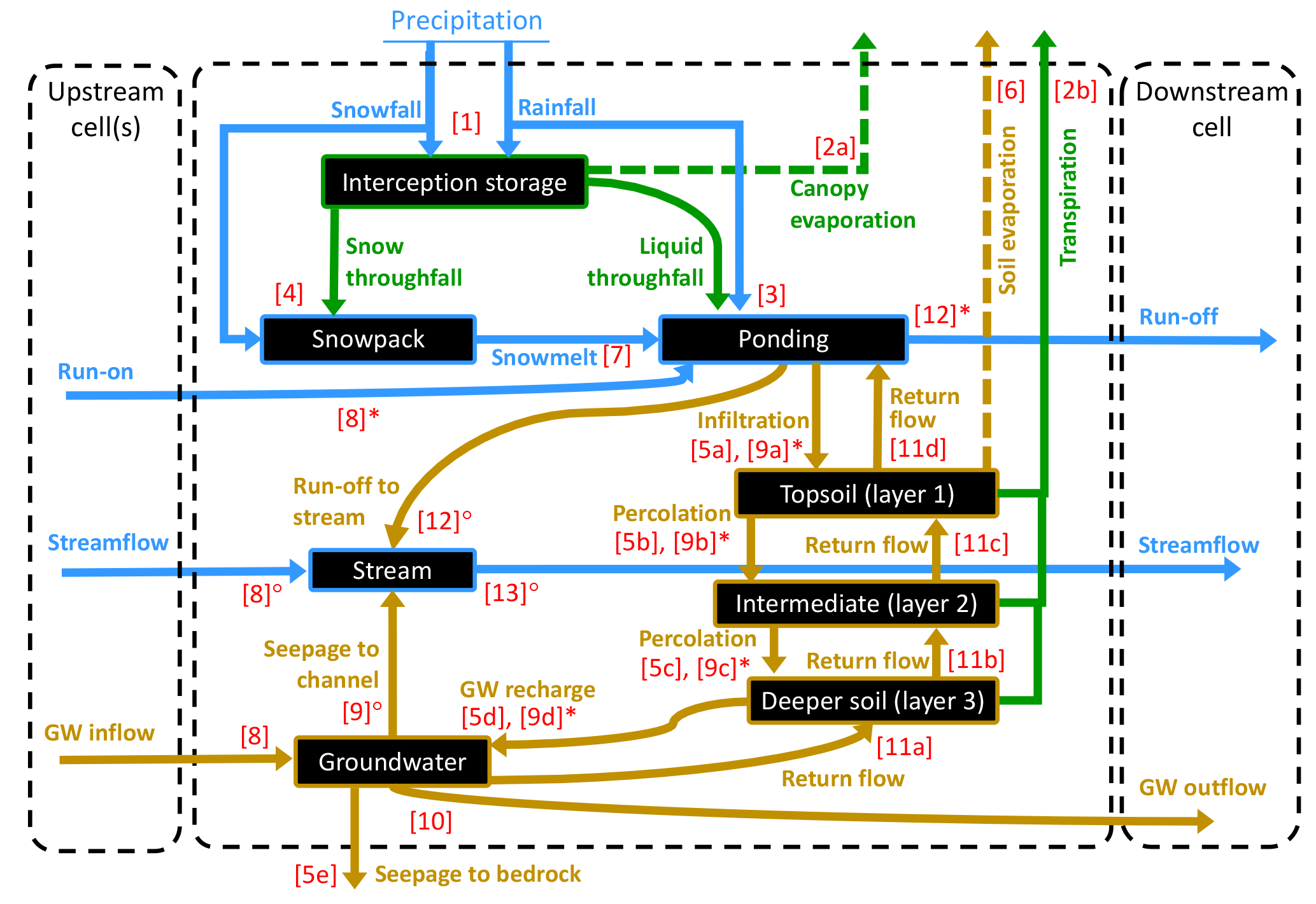
Figure 1Water compartments (black rectangles) and fluxes (coloured arrows) as represented in EcH2O-iso, with the dashed arrows indicating processes where isotopic fractionation is simulated. The numbers between brackets reflect the sequence of calculation within a time step. Note that water routing (steps 8 to 13) differs between cells where a stream is present (◦) or not (∗).
We provide here a brief step-wise overview, focused on the different hydrological compartments and transfers simulated in EcH2O at the grid cell level (Fig. 1). For each vegetation cover present in a grid cell, a linear bucket approach is used for canopy interception. The capacity-excess P (i.e. below-canopy throughfall) and P over bare soil are partitioned between liquid and snow components using a snow–rain temperature threshold (fixed to 2 ∘C) together with the minimum and maximum air temperatures at each time step. The canopy energy balance then separately yields plant transpiration (Et) and evaporation of intercepted water (Ec). The calculation of Et uses, for each vegetation type, the canopy conductance at each time step based on a Jarvis-type multiplicative model accounting for environmental limitations from incoming solar radiation, Ta, vapour pressure deficit at the leaf surface, and soil water potential (see Maneta and Silverman, 2013 and appendices in Kuppel et al., 2018a for a more detailed description). Infiltration of surface water in the topsoil layer is computed using a Green–Ampt approximation of the Richards equation. Subsequent soil water content above field capacity (gravitational water) percolates to the underlying soil layers, with fixed bedrock seepage – out of the system – as a lower boundary condition (Fig. 1). Soil evaporation (limited to the topsoil layer) and snowmelt (resulting in surface ponding; Fig. 1) under each vegetation type are calculated by solving the energy balance at the surface. Following a local drainage direction derived from the input elevation map, lateral water routing is simulated at three levels: in the deepest soil layer, groundwater seeps in the channel (if present) while the remainder is transferred laterally using a 1-D kinematic wave, and can result in saturation return flow in downstream cells. All remaining ponded water becomes overland flow, re-infiltrating further downstream or running off until it reaches an outlet or a cell within the stream network; stream water routing is also computed within a 1-D kinematic wave approximation.
2.2 Implementation of isotopic and age mixing
The conceptualisation of water mixing equally applies for all the tracked quantities implemented in the model (isotopes and age), so that a generic notation C is in this section used to designate both isotopic tracer composition (2H and 18O) and water age. The only specific conceptualisation of isotope dynamics in EcH2O-iso relates to fractionation (see Sect. 2.3), while precipitation inputs have a fixed age of zero and the water age in all compartments is increased at the end of each simulation time step by the length of the latter. The delta notation (δ) for isotopic composition quantifies, for a given water sample, the difference in the mass ratio of heavy to light isotopes (R) as compared to the Vienna Standard Mean Ocean Water (VSMOW): . First, the instantaneous mass balance for water signature is
where Vres and Cres are, respectively, the volume and signature (δ2H, δ18O, or age) of the water in the reservoir, t is time, qout is the flux of water exiting the reservoir, and qin,k and Cin,k are, respectively, the flux and signature of water entering the reservoir from each the Nin adjacent upstream locations. An implicit first-order finite-difference scheme is used to compute mixing during a given time interval Δt:
where and are, respectively, the volume and water signature in the reservoir after mixing, and are the volume and water signature in the reservoir before mixing, and is the signature of the kth input source after mixing in the latter. Replacing by in Eq. (2) finally yields
In practice, Eq. (3) is applied in EcH2O-iso at every sub-time step where water transfers are computed, in the sequence shown in Fig. 1. Note that in Eq. (3) only depends on the magnitude of the summed incoming flux . Flow to the downstream cell is fully mixed – right-hand terms of Eq. (2). Full mixing was used as a simplifying approximation because this model is to be first evaluated in a wet environment (Sprenger et al., 2017a; Tetzlaff et al., 2014) with relatively long time steps (i.e. daily; see Sect. 3.3). Note that because of its representation of a single, fully mixed pool in each soil layer, EcH2O-iso essentially provides bulk water values for isotopic content and water age. This needs to be kept in mind when comparing the simulations with soil isotopic datasets (see Sects. 3.2 and 4) and for the discussion (Sect. 5).
One exception to immediate mixing is the snowpack, where the snowmelt flux () is assumed to tap first into the snow throughfall of the same time step () if present, before mobilising older snow, fully mixed in the snowpack. Consequently, the signatures of the snowpack () and snowmelt water () which goes into the surface reservoir in EcH2O-iso at step 7 (Fig. 1) are calculated as follows:
Only the same-time-step precipitation can contribute to throughfall in the EcH2O model, whenever the resulting canopy storage exceeds the maximum canopy storage capacity (Maneta and Silverman, 2013), the latter being constant in our simulations. As a result, all intercepted water eventually evaporates from the canopy and does not interact with the surface/subsurface. Therefore, throughfall water (liquid and snow) is assumed to have the isotopic composition of same-time-step precipitation and age zero. This simplification is reasonable for our study site where vegetation interception has only a trivial effect on the isotopic partitioning of rainwater (Soulsby et al., 2017), yet further developments could be implemented for model application in different ecoclimatic settings.
Finally, transpiration is considered as a non-fractionating process. This is based on previous work (Dawson and Ehleringer, 1991; Harwood et al., 1999; Wershaw et al., 1966), and the fact that non-steady-state effects cancel out at the daily time step (Farquhar et al., 2007). However, this simple conceptualisation is increasingly questioned (Lin and da SL Sternberg, 1993; Vargas et al., 2017; Zhao et al., 2016), and the implications for our study will be discussed later. Here, during the canopy energy balance (step 2 in Fig. 1), the signature of transpired water is taken as the weighted sum of the signature in the three soil layers:
where fL1, fL2, and fL3 are the respective fractions of roots in each layer, as described in Eq. (A8) in Kuppel et al. (2018a).
2.3 Isotopic fractionation from soil evaporation
The change in isotopic composition of the first soil layer during soil evaporation (step 6 in Fig. 1) is simulated using the Craig–Gordon model Craig and Gordon (1965); Gat (1995), without any empirical parameterisation specific to our study. In this section, generically refers to the standardised isotopic ratio in for either 2H or 18O. For each time step t,
where f is the remaining fraction of water after evaporation (), while δ* is the limiting isotopic composition given the local atmospheric conditions in ‰(Gat and Levy, 1978) and m is the dimensionless enrichment slope (Allison and Leaney, 1982; Welhan and Fritz, 1977). Their formulation is generalised following Good et al. (2014):
The different terms in Eqs. (8) and (9) are sequentially defined as follows:
-
δa is the stable isotope composition of the ambient air moisture in ‰, derived from that of the precipitation by assuming isotopic equilibrium (Gat, 1995; Gibson and Reid, 2014):
-
ε+ is a factor (in ‰) derived from the equilibrium fractionation α+ of water between the liquid and vapour phases (Skrzypek et al., 2015):
with α+ taken as temperature dependent following Horita and Wesolowski (1994), here using the air temperature Ta:
-
εk accounts for the diffusion-controlled fractionation in air (Craig and Gordon, 1965):
where Di∕D is the diffusivity ratio of the gaseous water molecules bearing an isotope i to that of lighter isotopic water. We use literature values given by Vogt (1976), as suggested in Horita et al. (2008): 0.9877 for and 0.9859 for .
-
n translates the dominant mode of transport of water molecule at the surface. We adopted a time-varying formulation taking into account soil water content θ (Braud et al., 2005; Mathieu and Bariac, 1996):
where ϕ and θr are, respectively, the soil porosity and residual water content. n increases from 0.5 in a saturated soil to 1 for a dry soil where diffusion is the dominant mode of transport.
-
ha is the relative humidity of the atmosphere (measured at the weather stations; see Sect. 3.2) after being normalised to the saturated vapour pressure e* at the soil surface (Gat, 1995):
where the surface temperature Ts is given at each time step from solving the surface energy balance equation (Maneta and Silverman, 2013).
-
Finally, hs is the relative humidity of the air of the soil pores, following the formulation of soil evaporation flux Es in EcH2O (Maneta and Silverman, 2013):
where β is adjusted as a growing function of the volumetric water content θ, equal to 1 whenever θ is superior or equal to field capacity θfc (Lee and Pielke, 1992):
3.1 Study site
Simulations were conducted for the Bruntland Burn (BB) catchment in the Scottish Highlands (57∘8′ N, 3∘20′ W) (Fig. 2a and b). It is a small (3.2 km2) headwater catchment of the Dee, a major Scottish river providing freshwater resources for ∼250 000 people in the Aberdeen urban area, having EU conservation designations, and hosting ecosystem services (e.g. Atlantic salmon fishery). Annual precipitation averages around 1000 mm, with a mild seasonal cycle (Fig. 2c). The water balance is energy-limited, given the northern latitude, with 400 mm of annual evapotranspiration with pronounced seasonality in daily losses: from 0.5 mm in winter to 4 mm in summer (Birkel et al., 2011). Mean annual temperature is 7 ∘C and no monthly averaged temperatures fall below 0 ∘C; the climate qualifies as temperate to boreal oceanic; less than 5 % of precipitation usually occurs as snowfall.
Table 1Local datasets used in this study, grouped by location and purpose: model evaluation (▪), model calibration (▴), and model inputs (⧫). For soil isotopes, a and b, respectively, indicate suction-lysimetric sampling (2013) and direct equilibration from soil sampling (2015–2016). Other notations: Srf – surface water, GW – groundwater, P – precipitation, SWC – soil water content, Et – transpiration, NR – net radiation, * – relative air humidity, precipitation, air temperature, and wind speed, • – collection campaign at 92 to 94 locations (see text).
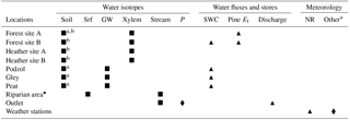
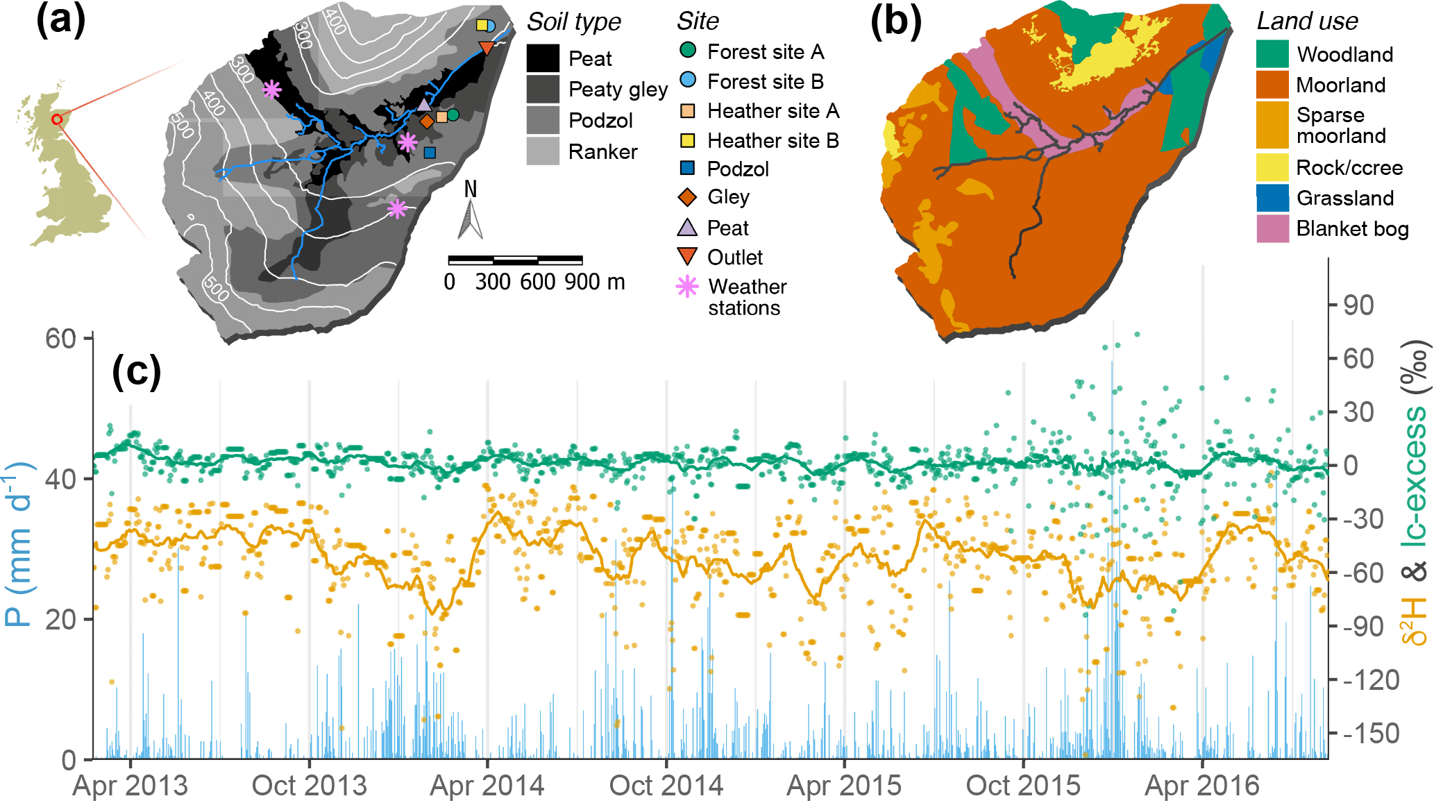
Figure 2Bruntland Burn catchment characteristics, showing (a) topography, soil cover as derived from the Hydrology of Soil Types (HOST) classification types, stream network, and measurement site locations, and (b) land use type. (c) Time series of measured precipitation amount (blue bars, daily) and isotopic signatures, δ2H (orange) and lc-excess (green), showing daily values (dots) and the 30-day running mean (solid lines).
The topography of the BB reflects glacier retreat, with elevation ranging from 220 m a.s.l. in the wide valley bottom to 560 m a.s.l. above the steeper slopes (Fig. 2a). Glacial drift deposits cover 60–70 % of the catchment bedrock (granite, schist, and other metasediments) and form the dominant soil parent material (Soulsby et al., 2007). Mostly saturated, these deposits are important reservoirs of groundwater, sustaining base flows in the stream and maintaining persistent wet conditions across the valley bottom (Soulsby et al., 2016). Thin Regosols (rankers) dominate the pedology of the catchment above 400 m a.s.l., where drift deposits are marginal (Fig. 2a). Freely draining shallow podzols (<0.7 m deep) dominate steeper hillslopes, overlying moraines and marginal ice deposits. Finally, deep (>1 m) soils with high organic matter content (Histosols: peat and gley) characterise the riparian area (Fig. 2a). The Histosols are saturated most of the time, so that rainfall events generate runoff mostly via rapid saturation overland flow, with a surface connectivity in the podzols limited to the wettest periods (Tetzlaff et al., 2014). Spatial patterns of land cover reflect these hydropedological units (Fig. 2b). Heather shrublands (Calluna vulgaris and Erica spp.) are the dominant cover over podzols and rankers. Such a land use results from red deer (Cervus elaphus) and sheep overgrazing, at the expense of naturally occurring Scots pine trees (Pinus sylvestris L.), which are now mostly found in the steep sections of the northern hillslopes and in the plantation areas neighbouring the stream outlet. Finally, grasses (Molinia caerulea) cover the riparian gley soils, while the peat is dominated by bog mosses (Sphagnum spp.).
3.2 Datasets
We used the wealth of diverse and often multi-year time series available at different locations in the BB catchment (Fig. 2a). These measurements capture numerous ecohydrological processes and observables, used either for model inputs or calibration/evaluation of simulations (Table 1). A brief description follows.
3.2.1 Isotopic measurements
At the catchment outlet, rainfall and stream water have been sampled daily for isotope analysis from June 2011 to the present, providing an isotope time series of unusual high frequency and longevity. Samples have been collected using an ISCO 3700 automatic sampler (Teledyne ISCO, Lincoln, USA). The auto-sampler bottles were emptied at fortnightly frequency or higher, while paraffin was added to each bottle to prevent evaporation.
Stable isotope measurements in the soil fall into two categories, differing in the sampling method and time period. Between 2011 and 2013, soil water was extracted at 0.1, 0.3, and 0.5 m depths at four locations: peat, gley, and podzol sites (weekly), and Forest site A (fortnightly) (Fig. 2a). Since MacroRhizon suction lysimeters were used (Rhizosphere Research Products, Wageningen, the Netherlands) (Tetzlaff et al., 2014), isotopic characterisation represents the mobile water held under lower tensions (Sprenger et al., 2015). From September 2015 to August 2016, near-monthly soil water sampling was carried out at four locations (Forest sites A and B, and Heather sites A and B) using soil samples collected with a spade from four layers (0–0.05, 0.05–0.1, 0.1–0.15, and 0.15–0.2 m) with five replicates for each. Isotopic analysis followed on water extracted by the direct equilibration method (Wassenaar et al., 2008), thus fully accounting for bulk pore water, as described by Sprenger et al. (2017a). Conceptually, the lysimeters can be viewed as sampling the “fast domain” of soil water held under low tension, whilst direct equilibration characterises the “bulk” soil water which also includes the “slow domain” of water held under higher tensions.
Groundwater samples were collected monthly between August 2015 and September 2016, at four wells (>1.6 m) covering a representative transect from the hillslope to valley bottom (Scheliga et al., 2017) encompassing the main hydropedological units: peat (two wells), gley, and podzol sites (Fig. 2a). Vegetation xylem water was collected between autumn 2015 and spring–summer 2016, using cryogenic extraction from Scots pine xylem cores at 1.5 m height (Forest sites A and B) and from heather twigs (Heather sites A and B) (Fig. 2a). Sampling was made at near-monthly resolution (n=7) with five replicas for each extraction (Geris et al., 2017). We also used isotopic measurements from a synoptic sampling campaign conducted in the drainage network of pools and channels across the valley bottom of the Bruntland Burn on 20 February (92 locations) and 24 May (94 locations) of the year 2013, covering contrasting catchment wetness states. On those days, water was also sampled along the perennial stream network at 10 locations (Lessels et al., 2016).
Air-tight vials were used to store all water samples, which were kept refrigerated until they were analysed. The soil samples were equilibrated and extracted water analysed within a week of collection (Sprenger et al., 2017a). In both cases, stable isotopic composition was determined using Los Gatos laser isotope spectrometers (DLT-100 and OA-ICOS models; Los Gatos Research, Inc., San Jose, USA), with reported measurement uncertainties of 0.4 and <0.55 ‰ (δ2H), and 0.1 and <0.25 ‰ (δ18O), respectively.
3.2.2 Hydrometric and meteorological data
Daily soil moisture data were derived from 15 min retrievals at four locations: three along the peat–gley–podzol transect presented in Sect. 3.2.1 (Tetzlaff et al., 2014), and in a Scots pine stand (Forest site B; Fig. 2a). Time domain reflectometry (TDR) soil moisture probes (Campbell Scientific, Inc. USA) were located at different depths (0.1, 0.3, and 0.5 m – only 0.1 and 0.3 m in the peat), and replicated ∼2 m apart. During two growing seasons, Scots pine transpiration was measured at Forest site A (July–September 2015) and at Forest site B (April–September 2016) (Fig. 2a), by installing Granier-type thermal dissipation sap flow sensors (Dynamax Inc., Houston, TX, USA) on 10 and 14 trees, respectively. Depending on its stem diameter (10 to 32 cm), each tree had two to four sensors. At the end of each study period, incremental wood core sampling in surrounding trees provided sapwood-area – tree-diameter relationships, used to derive stand-scale transpiration estimates (Wang et al., 2017a), which were then daily averaged. At the catchment outlet (Fig. 2a), 15 min stage height records (Odyssey capacitance probe, Christchurch, New Zealand) were used to generate daily discharge observations, with a rating curve previously calibrated for a stable stream section.
Finally, meteorological observations used as model inputs (P, Ta, relative humidity, and wind speed) and for calibration (net radiation) were primarily daily averaged from 15 min measurements at the three meteorological stations installed at different landscape positions (valley bottom, bog, and hilltop; Fig. 2a) and operated from July 2014. Prior to that period, a square elevation inverse distance-weighted algorithm was applied to interpolate local precipitation values from five Scottish Environment Protection Agency (SEPA) rain gauges located within 10 km of the Bruntland Burn catchment (Birkel et al., 2011). Daily mean Ta, relative humidity, and wind speed values were then available from the Centre for Environmental Data Analysis (CEDA) at the Balmoral station (∼5 km NW) (Met Office, 2017). The ERA-Interim climate reanalysis dataset (Dee et al., 2011) was used to retrieve daily minimum and maximum Ta (prior to July 2014), and incoming solar and longwave radiation (whole study period). Finally, we applied altitudinal effects on P and Ta were accounted for; we applied a 5.5 % increase of P every 100 m a.s.l. (Ala-aho et al., 2017), and a 0.6 ∘C decrease per 100 m a.s.l., from the moist adiabatic temperature lapse rate (Goody and Yung, 1995).
3.3 Model set-up and calibration
The methodology closely follows the approach detailed in Kuppel et al. (2018a). Here, we only provide a brief summary and highlight the modifications adopted for this study.
All simulations were performed on daily time steps, at a 100×100 m2 resolution. This choice of coarser grid cells – from 30×30 m2 in Kuppel et al. (2018a) – was made to decrease computation time while preserving reasonable spatial variability across the catchment. The simulation period extends from February 2013 to August 2016, for which a continuous record of daily δ2H and δ18O in precipitation input was available (see Sect. 3.2.1). For all simulations, a 3-year spin-up period was added using the first 3 years of isotopic and climatic model inputs, as preliminary sensitivity tests combined with visual inspection of simulated hydrometric and isotopic time series at the location used in this study (see Sect. 3.2) indicated it was sufficient to remove transient dynamics.
Based on the soil classes defined by the Hydrology of Soil Types (HOST), four hydropedological units were defined (Fig. 2a) (Tetzlaff et al., 2007) to map soil hydrological properties in the modelled domain. Physical soil characteristics relating to the energy balance were considered uniform across the catchment, similar to Kuppel et al. (2018a) (see Table S1 therein). Land cover was divided into five classes, four of them vegetated: Scots pine, heather shrubs, peat moss, and grasslands. From extensive land use mapping (Fig. 2b), the cover fraction of each vegetation type was estimated by combining 1×1 m2 resolution lidar canopy cover measurements (Lessels et al., 2016), aerial imagery, and typical vegetation patterns in the different soil units (Kuppel et al., 2018a; Tetzlaff et al., 2007). As in Kuppel et al. (2018a), the dynamic vegetation allocation module is switched off, so that leaf area index remains equal to initial values of 2.9, 1.6, 3.5, and 2 m2 m−2 for Scots pines, heather shrubs, peat moss, and grasslands, respectively (Albrektson, 1984; Bond-Lamberty and Gower, 2007; Calder et al., 1984; Moors et al., 1998). To avoid an overestimation of local soil evaporation and resulting isotopic fractionation in grid cells of exposed rock/scree, for simplicity, we fixed the depth of the first soil layer to 0.001 m wherever the fraction of bare soil was larger than 0.5 – after performing a sensitivity analysis showing little effect on catchment water balance and downstream isotopic budgets.
Finally, the calibrated model parameters (Table S1 in the Supplement), and associated sampling ranges, are those presented in Kuppel et al. (2018a). The parameter space was sampled using a uniform Monte Carlo approach. The corresponding 150 000 simulations were jointly constrained combining measurements of stream discharge, soil moisture (four sites), pine Et (two sites), and net radiation (three sites) (Table 1) whenever the observation periods overlapped with the current simulations (February 2013–August 2016; Fig. S1 in the Supplement). For soil moisture observations, a b-spline curve was fitted to the measured profile (to account for non-monotonic variations) on each sampling date, followed by a vertical integration. It enabled a consistent comparison against simulations in each of the upper two hydrological layers of EcH2O (see Fig. 1), while profile-averaged values were used for calibration in Kuppel et al. (2018a). Constraints were combined in a multi-criteria objective function based on the cumulative distribution functions (CDFs) of dataset-specific goodness of fit (GOF) (Ala-aho et al., 2017): mean absolute error for stream discharge and root mean square error for all others observations. This method allows retention of model parameter sets that give most behavioural simulations simultaneously across different variables (Kuppel et al., 2018a). We retained the 30 “best” of these parameterisations as a test bed for ensemble simulations of stable water isotopes and water age dynamics presented in this study.
3.4 Analysis
Daily, seasonal, and interannual climate variability result in changing isotopic composition of precipitation inputs. Equilibrium isotopic fractionation processes result in a strong correlation between rainfall δ2H and δ18O across the globe, defining a global meteoric water line (Dansgaard, 1964). At the BB catchment, there is a seasonal trend of more enriched values in summer and depleted in winter (e.g. Fig. 2c). A local meteoric water line (LMWL) was defined, using daily values from February 2013 to August 2016 and weighting by precipitation inputs (r2=0.96, p<0.001):

Figure 3Time series isotopic composition (δ2H – top, and lc-excess – middle) and soil volumetric water (bottom) at two sites located in the hillslopes: (a) one dominated by a heather shrub cover and (b) the other in a pine-dominated area. Black symbols and lines show measurements at a given depth while colours display the ensemble medians and 90 % intervals of simulations in the two uppermost soil layers, and the median mean absolute error (MAE) values between model and data are shown.
The line-conditioned excess (hereafter, lc-excess) was defined as the residual from the LMWL (Landwehr and Coplen, 2006):
with aLMWL=7.8, bLMWL=4.9 ‰ (Eq. 20). As oxygen has a higher atomic weight, non-equilibrium fractionation during the liquid- to vapour-phase change will preferentially evaporate (in terms of statistical expectation) 1H2H16O molecules rather than the heavy isotopologue 1H218O (Craig et al., 1963). The isotopic signature of a water sample affected by evaporation thus shows negative lc-excess values, as δ18O in non-evaporated water enriches faster than δ2H, and plots under the LMWL in the dual-isotope space (Landwehr et al., 2014). For these reasons, we preferred combining δ2H and lc-excess in our analysis (over separately looking at both δ2H and δ18O), to simultaneously highlight absolute isotopic dynamics and evaporative fractionation. Note that lc-excess was also preferred over the oft-used deuterium-excess, which translates the deviation of δ2H from the GMWL (Dansgaard, 1964). While the two quantities are mathematically similar, lc-excess displays much smaller seasonal dynamics from the near-0 ‰ value of precipitation inputs; thus, it advantageously allows separation of fractionation impacts from overall isotope dynamics (Sprenger et al., 2017a).
Similar to soil moisture observations, measured and simulated isotopic values in the soil are conceptually different: datasets are collected at specific depths (see Sect. 3.2.1), whilst model outputs provide average values for the different hydrological layers (Fig. 1). While original quantities were preserved for temporal analysis of the results, we additionally provided a formal quantification of model–data agreement. To do so, we reconstructed layer-integrated isotopic datasets at each soil sampling site, following the same interpolation–integration methodology used for soil moisture for computing model–data goodness of fit during calibration (Sect. 3.3).
As outlined in Sect. 1, our model evaluation is meant to test the ability of EcH2O-iso to generically simulate isotope dynamics across compartments. We used mean absolute error (MAE) to quantify model–data fit for all isotopic outputs, some of which present low temporal variability, have skewed distributions, or have a relatively lower sampling record, resulting in typical hydrograph-oriented efficiency metrics (Kling et al., 2012; Nash and Sutcliffe, 1970) being less applicable. The median values are shown on corresponding time series (Figs. 3–7), and normalised by each dataset range and used in conjunction with Pearson's correlation factor in Fig. 8 as a summary of model performance. The correlation coefficient axis in this dual model performance space represents the quality of the model in representing the variation of the data, while the normalised MAE axis provides information on the accuracy (bias) of the model.
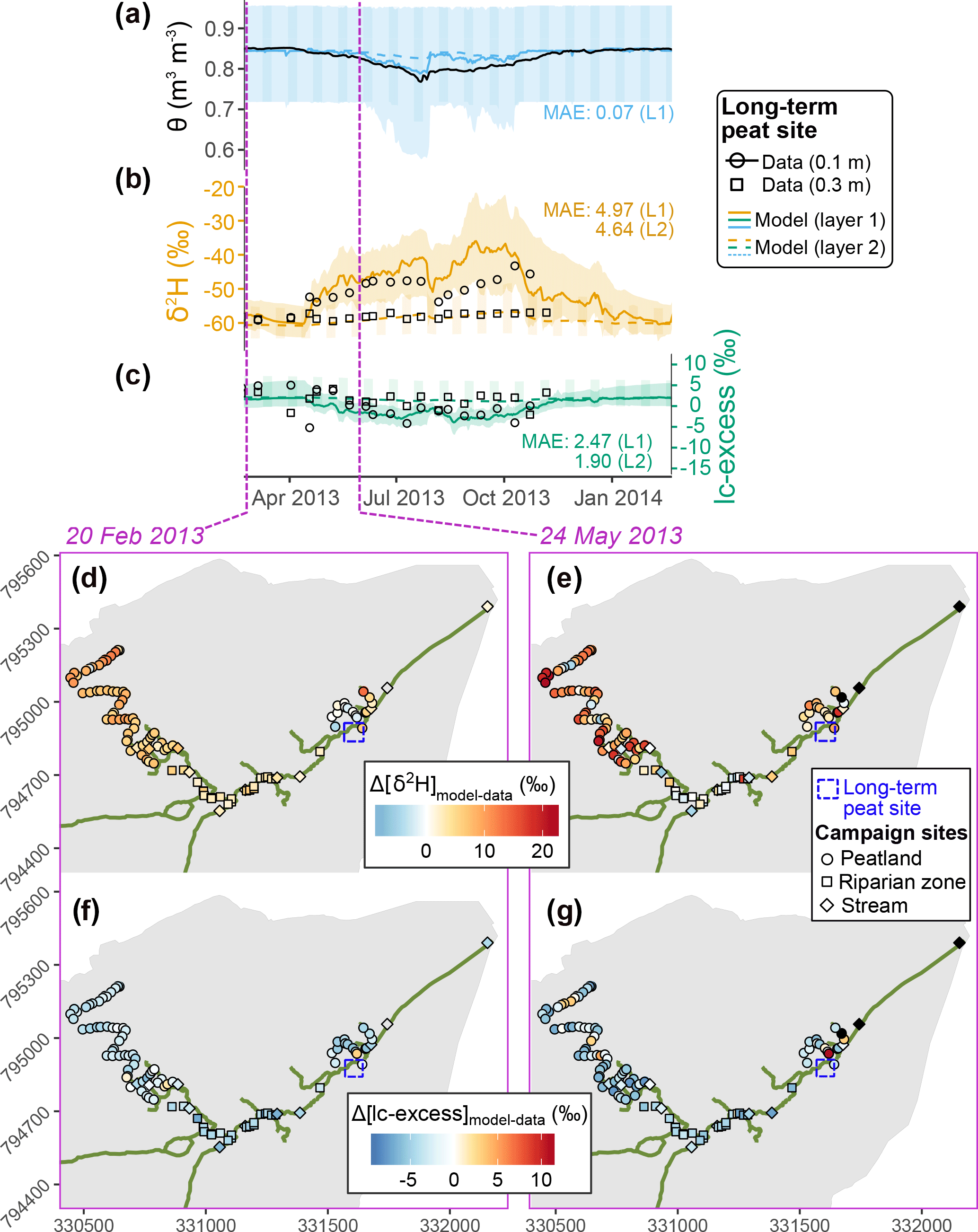
Figure 4(a–c) Time series of soil volumetric water content (θ) and isotopic composition (δ2H and lc-excess) at the peat site indicated by purple cross in the bottom maps. Measurements at a given depth are shown in black while colours display the ensemble medians and 90 % intervals of simulations in the two uppermost soil layers. (d–g) Model–data difference at two given days when samples were collected in the valley bottom, for deuterium (d–e) and lc-excess (f–g); black symbols indicate an absence of sample on one of the two dates, and the median model–data MAE values are shown.
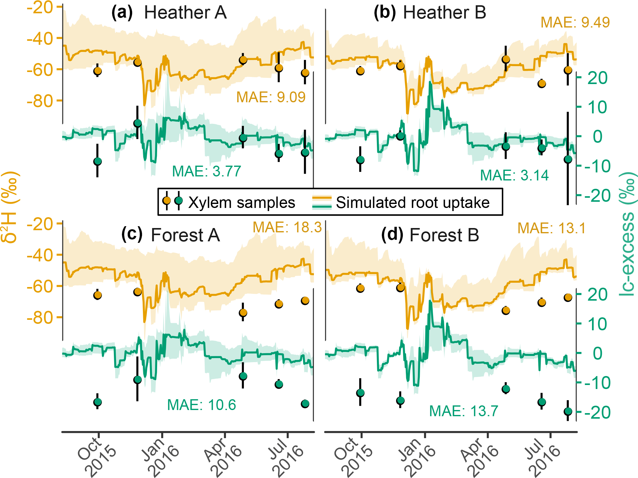
Figure 5Time series of deuterium composition (orange) and lc-excess (green) in the xylem of two heather shrublands (Heather sites A and B) and two Scots pine stands (Forest sites A and B). Measurements are shown with symbols with one standard deviation across replicas, while solid lines display ensemble medians and 90 % intervals of simulations, and the corresponding median model–data MAE values are shown.
4.1 Time series
Seasonal dynamics of soil water isotopes were well captured on the hillslopes, as exemplified at two sites in Fig. 3: one located in the shrub-dominated moorland (podzol site), the other in a Scots pine plantation (Forest site B), noting that the graphs cover different hydrological years dictated by data availability. Model–data agreement was consistent for δ2H, keeping in mind that while measurements were depth-specific, simulated values were averaged over the first and second hydrological layers (Fig. 1). As a result of model calibration (see Sect. 3.3), the thickness of the first (topsoil) and second layers spans 0.10–0.19 and 0.02–0.39 m in the simulated podzol soil unit, respectively (not shown). Still, at the podzol site the model captured well the vertical variability δ2H across the summer of 2013 but overestimated topsoil enrichment during the following winter (Fig. 3a). Lc-excess was generally underestimated in the topsoil layer there, with negative simulated values indicating evaporative influence generally not found in the data. At Forest site B, both δ2H and lc-excess dynamics showed modelled ranges consistent with measurements. Note, however, that EcH2O-iso simulated a vertical profile during the winter of 2016 with richer δ2H in the deeper layer, a condition that was only occasionally found in δ2H measurements (November 2015 and January 2016). At both sites, the temporal dynamics of soil moisture were well captured by the model (bottom rows). We note however that the observed decrease of moisture content with depth – especially marked at Forest site B – was generally not reproduced, as the vertically constant parameterisation of soil hydrology in EcH2O (Maneta and Silverman, 2013) does not allow sufficient water retention in highly organic upper soil layers.
Isotopic consistency was also found further in the valley bottom, as shown at the peat site in the riparian area (Fig. 4). The bimodal summer δ2H enrichment measured was well captured in the topsoil layer of the model (thickness: 0.02–0.25 m), as were the mildly negative lc-excess values. In addition, the weak variability and range of measured δ2H and lc-excess at greater depths were consistently reproduced. As for the podzol site, we noted in the peat higher peak enrichment values from the model than for the available data. As for other elements of the analysis, we remind here that soil isotopic data were sampled differently at the three sites: lysimeter extraction was used for the podzol and peat sites, therefore characterising mobile water in the fast domain, while the direct equilibration analysis conducted at Forest site B effectively applies to bulk water including water held under higher tension. The model essentially gives a bulk isotopic composition of stored water (Sect. 2), which might also explain why results were comparatively better at Forest site B.
We also explored the accuracy of simulated spatial patterns of isotopic signatures in the riparian zone, using two synoptic sampling surveys of surface water and stream water (Sect. 3.2.1) on separate days in late winter and late spring of 2013 (Fig. 4d–g). A good agreement was found for δ2H in the main branch of the stream network on both dates, while there was a tendency to overestimate δ2H values in the northwest part of the riparian area. Model–data fit of lc-excess mostly oscillated between good and a few per mille underestimation, depending on the location. For both δ2H and lc-excess there was fine-scale spatial variability in the model–data fit, especially marked in late May and in the main channel. This reflects both the spatial variability of measurements (Lessels et al., 2016; Sprenger et al., 2017b) and the different resolution of sampling (∼10 m intervals) and the much coarser grid of the simulations (100×100 m2).
Figure 5 shows EcH2O-iso's simulation of the isotopic imprint of plant water uptake in the transpiration flux. The isotopic composition of xylem water samples was directly compared to that of root water uptake simulated from the canopy energy balance (sub-step 2b in Fig. 1). At the heather sites, the simulated ranges were consistent from model to data, with an excellent model–data fit for lc-excess despite the low 90 % spread of simulations outputs (Fig. 5a and b). The seasonal cycle of simulated δ2H conversely seemed opposite to that of xylem samples, which showed gradual enrichment in winter followed by depletion at beginning of the growing season, but the lack of data from January to April limits general seasonal interpretation. At the forest sites, simulation results were very similar, noting that Forest site A corresponds to the same model grid cell as Heather site A (Fig. 5c and d). However, the measured isotopic composition in xylem was quite different for Scots pine compared to the heather, in two ways. First, the seasonal trends of δ2H were reversed, resulting in a good agreement with the modelled seasonality. Second, measured δ2H and lc-excess showed consistently lower values as compared to the heather sites, by 5 ‰–24 ‰ for δ2H and 4 ‰–13 ‰ for lc-excess (δ18O was only slightly positively biased, not shown). As a consequence, simulations showed a permanent positive offset for Scots pine water use despite consistent seasonality.

Figure 6Time series of deuterium composition (orange) and lc-excess (green) in groundwater at different locations in the catchment. Measurements are shown with symbols – with two wells on the same simulated peat grid cell, on opposite sides of the stream – while solid lines and ribbons show the median and 90 % confidence interval of ensemble simulations, and the median model–data MAE values are shown.
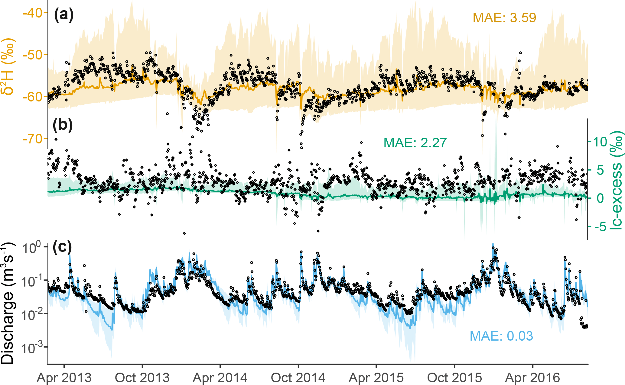
Figure 7Time series of stream isotopic composition – (a) δ2H and (b) lc-excess – and (c) discharge at the catchment outlet. Measurements are shown with black open symbols while colours display the medians and 90 % confidence intervals of ensemble simulations, and the model–data MAE values are displayed.
Isotopic variability was comparatively much lower for the groundwater both in time and across monitored wells, and a general agreement was found in the simulations (Fig. 6). The deuterium signal was robustly reproduced, with all measured values falling in the 90 % spread of simulation ensemble. However, the model tended to slightly underestimate lc-excess, with simulated values near zero while measurements were mostly centred on 3 ‰. In addition, the short-term lc-excess variability was somewhat underestimated in the riparian area.
Figure 7 shows the model–data comparison at the catchment outlet. The overall signal of stream water δ2H (Fig. 7a) and discharge values (Fig. 7c) were well reproduced by the model, with consistent “transition” periods of progressive enrichment when atmospheric demand increased and the catchment got drier. Most behavioural models in the ensemble did not completely capture the full extent of winter δ2H depletion, and the seasonal minimum of δ2H generally fell below the 90 % spread of the ensemble. However, seasonal variations of modelled lc-excess in the stream were in phase with the datasets throughout the study period: minimum in summer and maximum in winter, although simulated variability was more damped than for δ2H, with a slight negative bias (Fig. 7b).
A summary of model performance is shown in Fig. 8 for all sites/compartments, using the dual space of normalised MAE (using each dataset range, x axis) and Pearson's linear correlation factor (y axis). The vast majority of median normalised MAE values were below 1, and more than half of evaluated datasets showed values below 0.5. Values above 0.7 were mostly found for groundwater and xylem compartments, a clustering especially marked for δ2H. In addition, most median model–data correlations were significantly positive between 0.4 and 0.85, noting a tighter clustering around high values for δ2H than lc-excess. Insignificant or negative correlations were mostly found where only a few data points were available (xylem) or where seasonal variability was low (e.g. groundwater). Interestingly, median model–data agreement in topsoil at Forest site A significantly differed between 2013 (mobile water sampling via lysimeters) and the 2015–2016 period (bulk water sampling via direct equilibration). This was notable in the dramatic increase of model–data correlation (0.17 to 0.8) and decrease of normalised MAE (0.5 to 0.25) for topsoil δ2H in the latter case, which is consistent with our interpretation that the simulated soil water composition represents that of bulk water.

Figure 8Summary of model performance in the dual space of mean absolute error (normalised by the observed range of values) and Pearson's correlation factor between modelled and observed time series, for (a) δ2H and (b) lc-excess, showing the median and 90 % spread over the ensemble. The size of each symbol is proportional to the logarithm of the number of observation points available. Performance in soil compartments at Forest site A is further separated between the periods 2013 and 2015–2016 (the latter indicated with an asterisk), corresponding to two separate field data collection campaigns. Two groundwater wells are presents at the peat site.
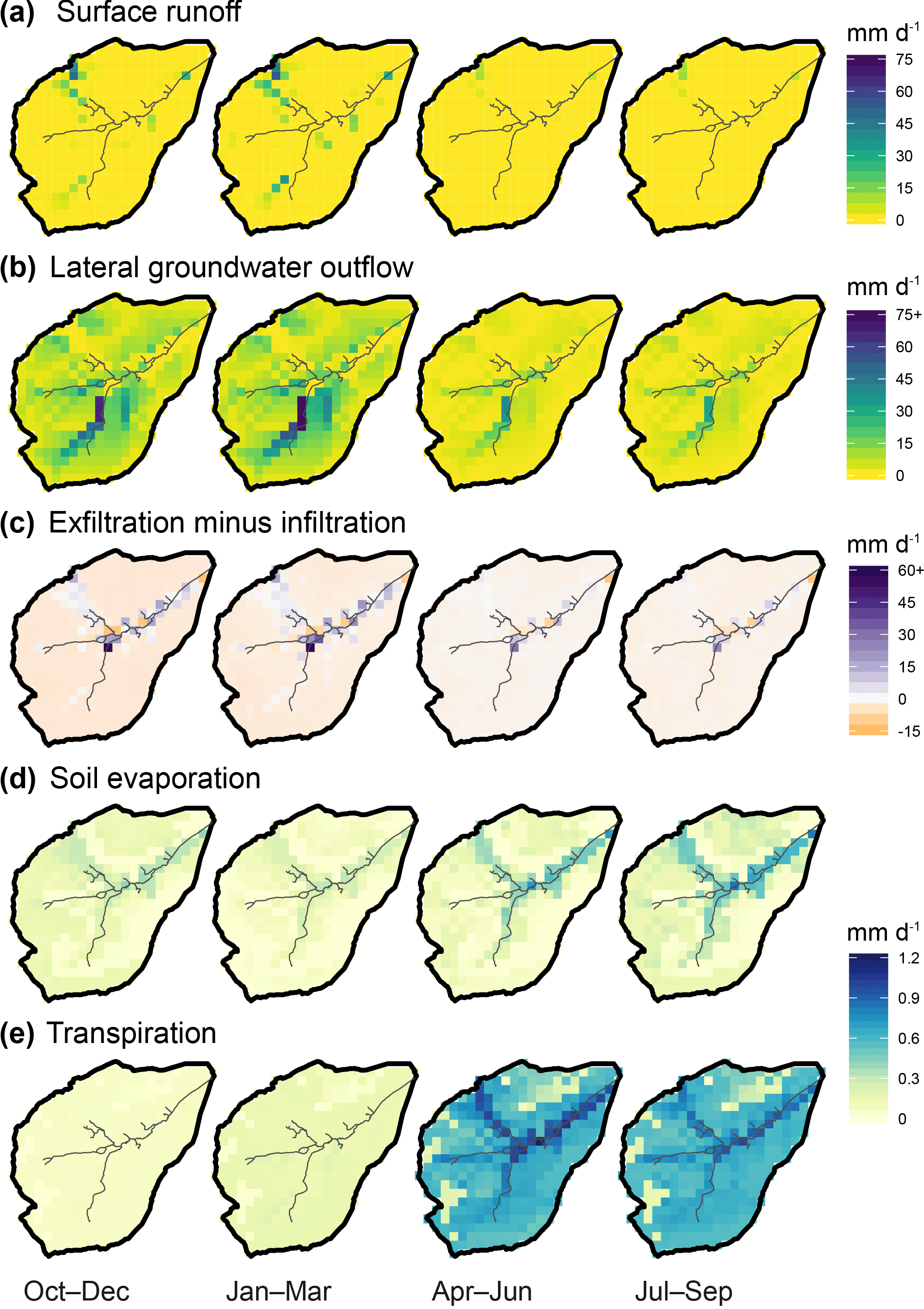
Figure 9Seasonally averaged daily outgoing water fluxes in the Bruntland Burn over the period 2013–2016, showing the ensemble median of simulated (a, b) cell-to-cell lateral flow, (c) net vertical liquid flow, and (d, e) evaporative losses via soil evaporation and transpiration, respectively.
4.2 Simulated hydrometric and isotopic spatial patterns
Figure 9 provides a spatially distributed, seasonal view of the ensemble median of outgoing water fluxes across the catchment over the simulation period. Lateral connectivity was markedly higher during the wetter first half of the hydrological year (October–March; Fig. 9a and b). During this colder, most energy-limited period, surface runoff – cumulative along the flow path, as runoff can cross several grid cells within one time step – was significant in many cells where the slopes transition to the valley bottom (up to 53 mm day−1, i.e. 0.006 m3 s−1), as well as on some surrounding hillslopes in the southern/southwestern part of the catchment (Fig. 9a). Throughout the spring–summer, very few of these overland flow corridors were usually hydrologically active, only in response to larger storm events. In parallel, lateral subsurface connectivity in autumn–wintertime was quite widespread across the catchment, particularly concerning the two southernmost stream tributaries where subsurface flux largely exceeded surface runoff (up to 90 mm day−1; Fig. 9b). Some of these subsurface connections were still active during the growing season, albeit weaker (<40 mm day−1). Given the predominance of subsurface flow near the channel, return flow dominated the vertical water budget (exfiltration minus infiltration >0) throughout the year at junctions with the main stream and further downstream, especially in the winter (Fig. 9c). The rest of the catchment was dominated by infiltration, with average net rates of a few mm day−1. Evaporative losses of soil water were much smaller and had a different seasonality than infiltration and throughflow (Fig. 9d and e). In autumn–winter, soil evaporation (Es) was similar in magnitude to ecosystem transpiration Et (integrated over all vegetation cover for each grid cell), although at local scales both fluxes remained below a few tenths of mm day−1 (catchment average: 0.11 mm day−1 for both Es and Et). Conversely, ecosystem transpiration clearly dominated during the rest of hydrological year, with a catchment-averaged rate almost 4 times higher than that of soil evaporation (0.61 mm day−1 vs. 0.16 mm day−1, respectively). In both cases, the highest values were found in the riparian area, although the spatial contrast was more marked for soil evaporation.
This spatiotemporal variability in water fluxes was somewhat reflected in that of isotopic patterns (δ2H in Fig. 10a, and lc-excess in Fig. S2). δ2H in the topsoil went from markedly depleted winter values (average: −61 ‰) to maximum enrichment in spring–summer with larger spatial variability (average: −44 ‰) (Fig. 10a). These temporal variations were well within that of δ2H in precipitation inputs (Fig. 2c). Yet, the increasing spatial variability of topsoil δ2H in spring–summer, and the much more pronounced relative seasonality of topsoil lc-excess (Fig. S2a) (compared to that in precipitation; Fig. 2c), indicated a significant influence of evaporation fractionation on isotopic patterns. During the spring–summer period the highest δ2H values, and most negative lc-excess values, were found in the organic soils of the valley bottom and on the higher hillslopes. These locations are where soil evaporation was highest (Fig. 9d) or where the soils are thinnest (rankers Regosols; Fig. 2a). The effect of isotopic fractionation crucially depends on relative storage change (Eq. 7); thus, it had large values either because absolute evaporation was high (valley bottom) or because the available storage was limited (thin soils). Conversely, spring–summer lc-excess values were near zero (or even slightly positive), and δ2H enrichment less pronounced, in most of the topsoil grid cells where the stream is also present, corresponding to the locations where upslope-routed groundwater exfiltrated (Fig. 9c). Finally, positive winter values for lc-excess across the catchment's topsoil hint at a widespread dominance of winter precipitation and mixing processes (via surface connectivity and infiltration; Fig. 9), over fractionating ones.
The isotopic signature (δ2H and lc-excess) in water used by plants for transpiration largely displayed a damped reflection of the topsoil patterns (Figs. 10a and S2a). This reflects distributed root uptake across the soil profile, reaching deeper soil compartments where seasonal isotope dynamics were less marked. One consequence is that the model simulated more isotopically depleted plant water use in the thin Regosols of the upper hillslopes compared to the very shallow topsoil layer (northern and western parts of the catchment).
Finally, groundwater δ2H patterns were comparatively more uniform across the catchment (σspatial=1.9 ‰) and across seasons (Fig. 10c). Most depleted values were found in the podzolic hillslopes and across the valley bottom, a feature more marked in winter and spring. Lc-excess mostly displayed positive values throughout the year, except for some weakly negative autumn values on the higher hillslopes (Fig. S2c). Markedly positive values were generally found in the organic soil of the valley bottom where fluxes converge. Note that positive values were more spatially homogeneous during winter and springtime, highlighting subsurface recharge lagging behind the more superficial compartments by a few months.
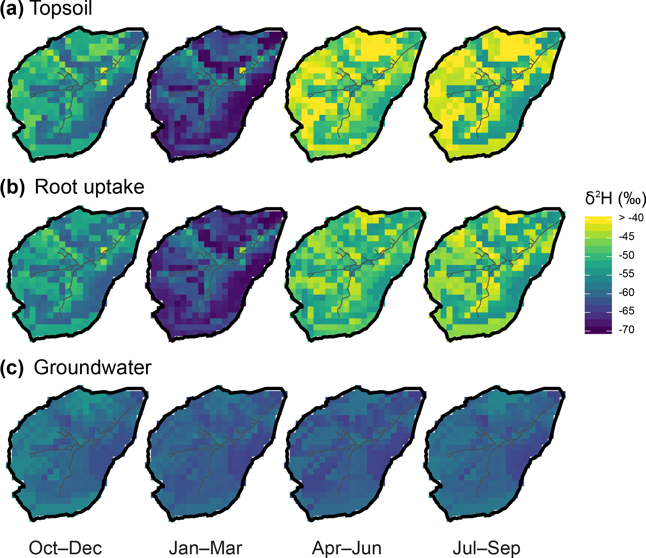
Figure 10Seasonal average of δ2H in the Bruntland Burn over the period 2013–2016, showing the ensemble median of simulations in (a) the topsoil layer, (b) root water uptake (summed of vegetation covers), and (c) groundwater.

Figure 11Ensemble median of simulated water age at the different sites used for model evaluation (except for Heather site A) in each corresponding compartment (a–d), and in the stream at several locations along the channel network (shown on the inset map, e). To improve visibility, all curves have been smoothed using a 7-day moving average window.
4.3 Water ages
Simulated water ages showed significant variability across locations in the catchment, as well as a marked seasonality at most sites selected for the analysis (Fig. 11). For convenience, the sites chosen for analysis in Fig. 11a–d were the same as those where isotopic model–data evaluation was conducted. In general, modelled water age increased with distance downhill, consistent with freely draining hillslopes sustaining groundwater fluxes into the riparian area. In the soils, water age ranged from a few weeks on the hillslopes to several years in the valley bottom peat where the topsoil is affected by exfiltration of older groundwater from upslope areas. Groundwater age was more homogeneous across the watershed but still showed significant differences, averaging 1 year in the podzol-covered locations, compared to 2 to 3 years in the riparian area. Seasonal variations were most significant on the hillslopes, from week-old waters in winter to water ages of 2 to 6 months during the growing season in the vadose zone. Weaker intrinsic seasonal variability was generally found in groundwater, which is consistent with the very flat simulated isotope dynamics (Fig. 6). The age of water taken up by plants followed the topsoil age patterns in most cases, reflecting the relatively young water ages from shallow rooting depths. One exception is Forest site A, where the contribution of older water from the second soil layer during the growing season had a clear effect on the age of the water used by vegetation. This latter site interestingly displayed older water ages compared to other hillslopes locations, suggesting slower drainage conditions, likely linked to less marked local topography and receipt of older water from upslope. In addition, the gley site displayed rather dynamic behaviour in the upper soil layers, similar to podzols, while the turnover of groundwater there was the lowest among all locations, suggesting it is confined and disconnected from the soil profile. Finally, at the peat site, younger water ages were found in groundwater compared to upper soil layers. This surprising result was likely linked to permanently saturated soils with limited infiltration (disconnection from the surface and overland flow) and recharge (disconnection from confined groundwater) where lateral soil water movement was not simulated, but lateral transfers and mixing occurred in the underlying groundwater.
Spatial variability was also found in stream water age, as shown in previously referred-to sites and arbitrarily defined locations along the channel network (Fig. 11e). In two of the main tributaries of the BB (HW2 and HW3), simulated water ages were significantly younger (∼0.5–1.5 years) than along the rest of the channel network (1.4–2.8 years). The older water ages found in HW1 might be linked to the presence of high water storage in drift deposits and an extensive raised peat bog in this portion of the valley bottom (Sprenger et al., 2017b), while the streams in HW2 and HW3 emerge further upslope at the drift-free ranker–podzol transition (Fig. 2a). There is a localised increase in water age when moving downstream towards the peat site, consistent with increased groundwater exfiltration (Fig. 9c) where stream water is a few weeks older than at the catchment outlet. In this lower part of the catchment lower temporal variability was also evident (1.8–2.4 years). Again, this might be derived from groundwater influxes and the extensive presence of saturated peat soils in this part of the catchment, compared to other sections of the stream.
5.1 Performance of the tracer-enhanced model
The model–data comparison demonstrated that EcH2O-iso captured a significant part of the isotopic behaviour across multiple ecohydrological compartments and landscape positions monitored in the study catchment. Because no calibration was performed on the isotopic components, these results reveal that the water mixing and storage and the water pathways simulated by the hydrologic core of EcH2O-iso correctly reflect the dominant hydrologic dynamics of the basin (Kuppel et al., 2018a). Hydrological states and fluxes in the model evolve driven by the celerity of propagation of local energy gradients (e.g. gravity-driven hydraulic gradient) throughout the landscape, with no direct knowledge about which “water parcels” (e.g. old or young, upslope or downslope) have been mobilised during a given hydrological response (Kirchner, 2003). Conversely, correctly capturing isotope dynamics is conditioned to accurately simulating patterns of water particle velocities, i.e. to routing the correct water parcels all the way from precipitation to their fate in the stream or as evaporative outputs (McDonnell and Beven, 2014). Therefore, the general performance achieved in the present celerity–velocity framework gives reasonable confidence in the mechanistic description of energy–water–plant couplings adopted by the EcH2O-iso model.
Despite some of the discrepancies presented and discussed below, the overall isotopic model–observation fit is very encouraging because the evaluated ensemble of model configurations was not derived from any tracer-aided calibration but solely used the information content brought by hydrometric and energy balance datasets in an independent calibration exercise similar to Kuppel et al. (2018a). Further, the implementation of water isotope and age tracking, consistent with the original structure of EcH2O and including evaporation fractionation of isotopes, was straightforward and followed well-established methodologies (Eqs. 4–18) without any parameterisation specific to the study site. By keeping both the isotopic module and calibration as minimalistic as possible, our approach avoids adding new, unnecessary degrees of freedom and reduces the risk of overfitting. Specific model performance might thus be lower than what could be achieved using a dual hydrometric-isotope calibration approach (Birkel et al., 2014; Knighton et al., 2017; van Huijgevoort et al., 2016), but because the isotopic signal remains truly independent of the hydrologic calibration our approach allows unique critical analysis and insight into the physical hypotheses underlying simulated flow generation and water mixing.
5.2 Insights into critical processes for model future development
The timing of seasonal isotopic dynamics as well as higher-frequency responses was well simulated in the vast majority of cases (summary in Fig. 8), together with value ranges also broadly consistent with observations. Yet, the amplitudes of modelled temporal isotopic responses displayed variable degrees of agreement with that of measured signals. In general, dynamics of deuterium were better reproduced than those of lc-excess, with a trend to underestimate lc-excess in several compartments.
One of these model–data mismatches is the overly enriched signal in the topsoil of the riparian sites during the growing season (Figs. 4 and 8). The concomitant underestimated lc-excess hints at an excessive evaporation fractionation signal. As pointed out in Sect. 4.1, these discrepancies can partially derive from the different information represented by model and observations. For instance, the model simulates the composition of the bulk topsoil water, whereas the observations may reflect only the composition of the free draining portion of the soil water. At the long-term riparian locations (peat and gley sites; Fig. 2a), collection by suction lysimeters (Tetzlaff et al., 2014) was used, sampling water under low tension and less affected by fractionation (Brooks et al., 2010; Sprenger et al., 2017b). In addition, the samples from a synoptic field campaign across the extended riparian area in flowing surface waters and ponds on two dates (Lessels et al., 2016) were directly compared to simulated topsoil water (Fig. 4d–g). This was because the current formulation of EcH2O-iso routes all surface water to the next downstream cell and thus does not account for free-standing water such as the ponds and zero-order streams typically forming outside summer in the BB, particularly in the northwest of the catchment (Lessels et al., 2016). Yet, the sampled surface water in the riparian area has been shown to have spatially varying sources, presenting distinctively enriched or depleted δ2H signals depending if the source is soil water or groundwater, respectively (Lessels et al., 2016). Systematically comparing soil water to sampled surface water might thus explain the overestimation of δ2H, especially in the northwest part of the catchment where limited groundwater seepage is modelled (Fig. 9c). Secondly, the riparian topsoil in EcH2O-iso might function as an “evaporation hotspot” to a greater extent than has been found in corresponding sampled surface water locations (Sprenger et al., 2017b). Indeed, topsoil water is not laterally connected in the model, so that evaporation fractionation remains local (horizontally) but immediately mixes across the whole layer – as compared to a vertically stratified isotopic profile in poorly mixed ponded areas. In addition, while fractionation is modest compared to other climatic settings, measurements have shown that ponds and zero-order channels that are not fully evaporated connect to the channel network in spring–summer and drive the seasonal isotopic enrichment observed in the stream (Sprenger et al., 2017b). Further support for this hypothesis was found by disabling evaporative fractionation in our simulations: seasonal variability of isotopes in the stream almost completely disappeared, while short-term, event-driven dynamics remained (not shown). Beyond the idiosyncrasies of our study catchment, and the gap between fine-scale wetland heterogeneity and our model resolution (100×100 m2), a large body of literature has reported the importance of riparian wetlands as time-varying “chemostats” controlling stream water quality (Billett and Cresser, 1992; Smart et al., 2001; Spence and Woo, 2003) or “isostats” mixing isotope signals (Tetzlaff et al., 2014). Since modelled soil water is not laterally routed to the channel during the onset of the growing season, this might explain some underestimation of summer δ2H in the stream outlet, as well as the reported lack of seasonal variability for instream lc-excess (Fig. 7). Further developments of the model to include ponding effects and/or a more dynamic channel network (rather than fixed, as currently conceptualised) would help capture these seasonally varying flow paths in the variably saturated valley bottom of low-energy landscapes.
The isotope and age tracking adopts a complete and instantaneous mixing scheme at each sub-time step where water transfers are computed between the spatially distributed compartments of the simulated domain. This working hypothesis was chosen for simplicity, given the wet and cool climate conditions and the relatively long (daily) simulation time steps. The spatiotemporal variability of simulated fluxes and stores somewhat results in a time-variant partial mixing at the catchment scale at the stream outlet (van Huijgevoort et al., 2016). However, we note, for example, that our simulations of groundwater lc-excess showed an underestimated variability and a consistent negative bias towards near-zero values (Fig. 6). It indicates that the simulated recharge signal is very damped throughout the year and slightly biased towards the signature of over-enriched, evaporation-affected recharge. This contrasts with the evidenced dominance of winter recharge given the markedly positive lc-excess values observed at the monitored wells (Scheliga et al., 2017) as well as in other catchments with comparable ecoclimatic settings (Bertrand et al., 2014; O'Driscoll et al., 2005; Yeh et al., 2011). It might point to an exaggerated mixing across the soil profile in our simulations, overly flattening the precipitation signature and overestimating fractionation signal in the water percolating to the water table. Given that groundwater directly sustains 19 (±16) % of annual stream flow in our ensemble simulations (not shown), one can link this lack of variability in groundwater lc-excess to that simulated in stream water (Fig. 7). While such a link between the degree of unsaturated zone mixing and stream isotopes was not evidenced by Knighton et al. (2017), there was a much lower contribution of baseflow to discharge in the intermittent catchment they modelled. More generally, further developments would benefit from incorporating insights from the growing body of literature on the importance of preferential flow in driving catchment dynamics and tracer mixing (Beven and Germann, 2013). This would first involve implementing conceptualisation of microtopographic controls on overland flow (Frei et al., 2010). Secondly, the significance of subsurface dual pore space (matrix–macropore) representations of tracer flow paths and mixing has long been put forward (Beven and Germann, 1982) but modelling efforts relevant to catchment hydrology remain somewhat scarce (Smith et al., 2018; Sprenger et al., 2018; Stumpp and Maloszewski, 2010; Stumpp et al., 2007; Vogel et al., 2010). Bridging these detailed plot- to hillslope-scale descriptions with a physically based ecohydrological model such as EcH2O-iso will likely require a simplified, parsimoniously parameterised implementation and calibration with tracer data.
Our modelling experiment also helps to evaluate the conceptualisation of isotopic fractionation in the soil water of wet, energy-limited catchments. The evaporative fractionation is described by the well-established Craig–Gordon model (Craig and Gordon, 1965), supplemented here with a soil-adapted formulation following Mathieu and Bariac (1996) and Good et al. (2014). As reviewed by Horita et al. (2008), the Craig–Gordon model is very sensitive to the isotopic composition of atmospheric moisture (δa), the relative humidity of the atmosphere at the surface (ha), and the kinetic fractionation factor (ϵk). We assumed isotopic equilibrium between rainfall and atmospheric moisture (Eq. 10), as is commonly done when no direct measurement of δa is available (Horita et al., 2008). While this empirical, and here spatially uniform, approach is valid on monthly timescales in temperate climates (Jacob and Sonntag, 1991; Schoch-Fischer et al., 1983), discrepancies can arise on shorter timescales and/or when local evaporation significantly feeds atmospheric moisture (Krabbenhoft et al., 1990). Second, ha estimates can be a large source of error in wet environments where ha>0.75 (Kumar and Nachiappan, 1999), which is often the case in our catchment (Wang et al., 2017b). Furthermore, we found a marked sensitivity of isotope dynamics to the strategy used to calculate ϵk (Eq. 14), consistent with Haese et al. (2013), who found a large impact on simulated soil δ18O in northern latitudes. We chose to use a formulation based on isotopic diffusivity ratios; the latter were taken from Vogt (1976) because their experimental protocol covered a comparatively large range of humidity conditions. Yet it seems that very few (if any) experimental studies estimating these ratios spanned the very humid conditions found at the BB, and further empirical data could help reduce the associated uncertainties (Horita et al., 2008).
Finally, we showed that our root uptake simulations for heather shrubs broadly matched the measured isotopic signature in plant xylem. Conversely, a systematic, positive model offset was found for both δ2H and lc-excess in Scots pines despite the fact that the model correctly captured the temporal dynamics (Fig. 5). Our simulations assumed identical, exponential root profiles for all vegetation types within soil types, e.g. the podzol, where these experimental heather and forest sites are found (Kuppel et al., 2018a); thus, species-dependent use of soil water from depth-specific isotopic signature cannot be captured. Heather shrubs have, however, a shallow root system (Geris et al., 2017), and thus its source water might be more affected by evaporation than Scots pine (which can be deeper rooted). However, the observed lc-excess values in the soil of Scots pine (−13 to 5.5 ‰; Fig. 3b, Forest site A not shown) were significantly higher than those measured in the pine xylem (−19.6 to −7.6 ‰; Fig. 5c and d). It mostly seems to stem from significant recorded deuterium depletion while 18O ratios were consistent or slightly depleted as compared to soil samples, and we found larger simulation biases (relative to the mean value) in xylem for deuterium than for 18O ratios (not shown). Such isotopic departures between soil and xylem water have been reported in a number of experimental studies, although primarily conducted in seasonally drier environments (Lin and da SL Sternberg, 1993; Vargas et al., 2017; Zhao et al., 2016). Several mechanisms have been proposed, including a discrimination of heavier isotopes during water uptake controlled by root aquaporins (Mamonov et al., 2007) or mycorrhizal associations (Berry et al., 2017), phloem–xylem water cycling on several timescales (De Schepper and Steppe, 2010; Hölttä et al., 2006; Pfautsch et al., 2015; Stanfield et al., 2017), and stem water evaporation through the bark (Dawson and Ehleringer, 1993). While exploring the relevance of these mechanisms to the ecosystems here simulated goes far beyond the scope of this study, it is clear that the complexity of isotopic dynamics in plant xylem cannot be fully captured simply based on a root-profile-weighted mixing of soil pools.
5.3 Opportunities for characterising water pathways
The development of EcH2O-iso is a methodological “middle path” for modelling conservative tracer transport, between detailed plot-scale models across the soil–vegetation–atmosphere continuum (Braud et al., 2005; Haverd and Cuntz, 2010; Mathieu and Bariac, 1996; Melayah et al., 1996), catchment rainfall–runoff models (Birkel and Soulsby, 2015; Knighton et al., 2017; McGuire and McDonnell, 2015; van Huijgevoort et al., 2016), and land surface models for Earth system studies (Haese et al., 2013; Risi et al., 2016; Wong et al., 2017). This reflects the reasons why the original EcH2O model was developed, namely to provide a physically based, yet computationally efficient representation of energy–water–ecosystem couplings where intra-catchment connectivity (both vertical and lateral) could be explicitly resolved (Maneta and Silverman, 2013). The combination of these features is critical, since explicit lateral connectivity (surface, subsurface, and channel) is typically the missing piece in land surface models (Fan, 2015) and in plot-scale approaches, and the coupling with vegetation processes is typically missing in rainfall–runoff models (van Huijgevoort et al., 2016). The newly developed model provides, for the first time, a transferable, process-based linkage of spatial–temporal patterns of water fluxes (Fig. 9) with those of isotopic tracers (Figs. 10 and S2) across a headwater catchment.
Here, a major focus has been put on the isotopic analysis to evaluate the consistency of EcH2O-iso using the wealth of data available at the study site, and the limitations stemming from the unavoidable technical trade-off we adopted. Yet, principles used for isotope tracking were applied to track water age across the ecohydrological compartments (Fig. 11). This provides a more complete picture of catchment functioning than stream water age, although the latter metric provides an important first-order benchmark for comparison with other modelling approaches. The mean stream water age of ∼2.1 years is consistent with isotope-calibrated rainfall–runoff approaches reporting ∼1.55 years (Ala-aho et al., 2017; van Huijgevoort et al., 2016) and ∼1.8 years (Soulsby et al., 2015). The low temporal variability found here yields higher discrepancies when considering flow-weighted median ages: ∼2 years against 1.2 years found by Soulsby et al. (2015) and ∼1 year reported using transport model driven by StorAge Selection functions (Benettin et al., 2017). We notably find a slower water turnover in the valley bottom soils (∼2.8 years) as compared to compared to the spatially distributed approach of van Huijgevoort et al. (2016) (∼2 years), and EcH2O-iso conversely simulates much younger water ages in the groundwater both on the hillslope and in the valley bottom (∼0.9 and ∼2.2 years vs. ∼2.9 and ∼3.4 years, respectively) and on the hillslope soils (∼0.2 years vs. ∼0.8 years) than van Huijgevoort et al. (2016). Keeping in mind that these discrepancies might arise from differences in modelling and calibration approaches, these mismatches may also confirm a tendency of EcH2O-iso to overemphasise the role of the riparian area as a hydrologic buffer and mixing zone, as well as the contribution of groundwater, in damping the stream isotope response which could be addressed by strategies suggested in preceding sections.
The EcH2O-iso model presented in this study is, to our knowledge, the first to simulate catchment dynamics of water isotopes (2H and 18O) and age by combining a physically based description of hydrological stores and fluxes, a spatially distributed simulation domain, a predictive vegetation component, and non-conservative isotopic processes (evaporative fractionation). Evaluated against a multi-site, extensive isotopic dataset encompassing a wide range of ecohydrological compartments (soil moisture, groundwater, plant xylem, and stream water) across hydropedological units, the model has generally shown good performance in reproducing the seasonal and higher-frequency variations of absolute and relative isotopic content (δ2H and lc-excess, respectively). Despite some limitations, this isotope-based evaluation suggests a reasonable capture of the velocity fields (i.e. how fast water parcels move) across the catchment, and complements a previous calibration and evaluation mostly using hydrometric observations (water fluxes and storage dynamics) which indicated a good simulation of catchment functioning from a celerity viewpoint (i.e. how fast energy propagates via the hydraulic gradient) (Kuppel et al., 2018a). Satisfying this dual velocity–celerity perspective is key to characterising water pathways and quantifying the associated travel times in different ecohydrological compartments of headwater landscapes. Complementing more conceptual approaches, the physical basis of the EcH2O-iso model further provides the potential to extrapolate these insights beyond recorded conditions and scales, and to notably project the reciprocal feedbacks between plant water use, hydrological pathways, and potential environmental changes. The relatively simple conceptualisation of compartment-scale velocities, e.g. assuming complete mixing and without site-specific parameterisation, and the absence of isotopic calibration, already make the current results particularly encouraging. It also provides a useful framework for hierarchising model development and benchmarking needs. For example, some of the model–data discrepancies in our results stress the necessary incorporation of partial mixing hypotheses, likely to be critical in drier and/or flatter landscapes where diffusive water movement prevails. Second, our model–data analysis of isotope dynamics strongly reflects fractionation effects, be it via soil evaporation or species-specific plant water use. Finally, the versatility of climatic settings in which the original EcH2O model has already been evaluated facilitates applying the presented methodology beyond the specifies of a high-latitude, low-energy, wet and steep headwater catchment such as the one simulated here. Further, the flexible spatial domain used by the model will help to provide a process-based modelling framework for plot- to catchment-scale hypothesis testing. This is timely for current challenges in critical zone science, such as exploring the occurrence and mechanisms behind the postulated ecohydrological separation of water fluxes (Berry et al., 2017).
The source code of the EcH2O-iso model used in this study corresponds to the branch master_1.0 in Kuppel (2017). The presented datasets are available from the PURE data repository of the University of Aberdeen (Kuppel et al., 2018b).
The supplement related to this article is available online at: https://doi.org/10.5194/gmd-11-3045-2018-supplement.
SK developed the EcH2O-iso code as a fork of the EcH2O code, with help from MPM. SK performed model simulations and prepared the paper. All authors discussed the results and contributed to the text.
The authors declare that they have no conflict of interest.
This work was funded by the European Research Council (project
GA 335910 VeWa). Marco P. Maneta acknowledges support from the US National
Science Foundation (project GSS 1461576) and US National Science Foundation
EPSCoR cooperative agreement no. EPS-1101342. We thank the topical editor
(Min-Hui Lo), Jr-Chuan Huang, two anonymous reviewers for their
suggestions which significantly improved the paper, and Aaron A. Smith
for fruitful discussions regarding the model development. We also acknowledge
the support of the Maxwell computer cluster funded by the University of
Aberdeen. Finally, we are grateful to the many people who have been involved
in establishing and continuing data collection at the Bruntland Burn,
particularly Christian Birkel, Maria Blumstock, Jon Dick, Josie Geris,
Konrad Piegat, Bernhard Scheliga, Matthias Sprenger, Claire Tunaley, and
Hailong Wang.
Edited by: Min-Hui Lo
Reviewed by: Jr-Chuan Huang and two anonymous referees
Ala-aho, P., Tetzlaff, D., McNamara, J. P., Laudon, H., and Soulsby, C.: Using isotopes to constrain water flux and age estimates in snow-influenced catchments using the STARR (Spatially distributed Tracer-Aided Rainfall–Runoff) model, Hydrol. Earth Syst. Sci., 21, 5089–5110, https://doi.org/10.5194/hess-21-5089-2017, 2017. a, b, c, d, e
Albrektson, A.: Sapwood basal area and needle mass of Scots pine (Pinus sylvestris L.) trees in central Sweden, Forestry, 57, 35–43, 1984. a
Allison, G. B. and Leaney, F. W.: Estimation of isotopic exchange parameters, using constant-feed pans, J. Hydrol., 55, 151–161, https://doi.org/10.1016/0022-1694(82)90126-3, 1982. a
Barnes, C. J. and Bonell, M.: Application of unit hydrograph techniques to solute transport in catchments, Hydrol. Process., 10, 793–802, 1996. a
Benettin, P., Soulsby, C., Birkel, C., Tetzlaff, D., Botter, G., and Rinaldo, A.: Using SAS functions and high-resolution isotope data to unravel travel time distributions in headwater catchments, Water Resour. Res., 53, 1864–1878, 2017. a, b
Berry, Z. C., Evaristo, J., Moore, G., Poca, M., Steppe, K., Verrot, L., Asbjornsen, H., Borma, L. S., Bretfeld, M., Hervé-Fernández, P., Seyfried, M., Schwendenmann, L., Sinacore, K., De Wispelaere, L., and McDonnell, J.: The two water worlds hypothesis: Addressing multiple working hypotheses and proposing a way forward, Ecohydrology, 11, e1843, https://doi.org/10.1002/eco.1843, 2017. a, b
Bertrand, G., Masini, J., Goldscheider, N., Meeks, J., Lavastre, V., Celle-Jeanton, H., Gobat, J.-M., and Hunkeler, D.: Determination of spatiotemporal variability of tree water uptake using stable isotopes (δ18O, δ2H) in an alluvial system supplied by a high-altitude watershed, Pfyn forest, Switzerland, Ecohydrology, 7, 319–333, 2014. a
Beven, K. and Germann, P.: Macropores and water flow in soils, Water Resour. Res., 18, 1311–1325, 1982. a
Beven, K. and Germann, P.: Macropores and water flow in soils revisited, Water Resour. Res., 49, 3071–3092, https://doi.org/10.1002/wrcr.20156, 2013. a
Billett, M. F. and Cresser, M. S.: Predicting stream-water quality using catchment and soil chemical characteristics, Environ. Pollut., 77, 263–268, 1992. a
Birkel, C. and Soulsby, C.: Advancing tracer-aided rainfall–runoff modelling: a review of progress, problems and unrealised potential, Hydrol. Process., 29, 5227–5240, https://doi.org/10.1002/hyp.10594, 2015. a, b, c
Birkel, C., Tetzlaff, D., Dunn, S. M., and Soulsby, C.: Using time domain and geographic source tracers to conceptualize streamflow generation processes in lumped rainfall-runoff models, Water Resour. Res., 47, W02515, https://doi.org/10.1029/2010WR009547, 2011. a, b, c
Birkel, C., Soulsby, C., Tetzlaff, D., Dunn, S., and Spezia, L.: High-frequency storm event isotope sampling reveals time-variant transit time distributions and influence of diurnal cycles, Hydrol. Process., 26, 308–316, 2012. a
Birkel, C., Soulsby, C., and Tetzlaff, D.: Developing a consistent process-based conceptualization of catchment functioning using measurements of internal state variables, Water Resour. Res., 50, 3481–3501, https://doi.org/10.1002/2013WR014925, 2014. a, b
Birkel, C., Soulsby, C., and Tetzlaff, D.: Conceptual modelling to assess how the interplay of hydrological connectivity, catchment storage and tracer dynamics controls nonstationary water age estimates, Hydrol. Process., 29, 2956–2969, 2015. a, b
Bond-Lamberty, B. and Gower, S. T.: Estimation of stand-level leaf area for boreal bryophytes, Oecologia, 151, 584–592, https://doi.org/10.1007/s00442-006-0619-5, 2007. a
Botter, G., Bertuzzo, E., and Rinaldo, A.: Transport in the hydrologic response: Travel time distributions, soil moisture dynamics, and the old water paradox, Water Resour. Res., 46, W03514, https://doi.org/10.1029/2009WR008371, 2010. a
Braud, I., Bariac, T., Gaudet, J. P., and Vauclin, M.: SiSPAT-Isotope, a coupled heat, water and stable isotope (HDO and H2 18O) transport model for bare soil. Part I. Model description and first verifications, J. Hydrol., 309, 277–300, 2005. a, b, c
Braud, I., Bariac, T., Biron, P., and Vauclin, M.: Isotopic composition of bare soil evaporated water vapor. Part II: Modeling of RUBIC IV experimental results, J. Hydrol., 369, 17–29, 2009. a
Brooks, J. R., Barnard, H. R., Coulombe, R., and McDonnell, J. J.: Ecohydrologic separation of water between trees and streams in a Mediterranean climate, Nat. Geosci., 3, 100–104, 2010. a
Brooks, P. D., Chorover, J., Fan, Y., Godsey, S. E., Maxwell, R. M., McNamara, J. P., and Tague, C.: Hydrological partitioning in the critical zone: Recent advances and opportunities for developing transferable understanding of water cycle dynamics, Water Resour. Res., 51, 6973–6987, 2015. a
Calder, I. R., Hall, R. L., Harding, R. J., and Wright, I. R.: The use of a wet-surface weighing lysimeter system in rainfall interception studies of heather (Calluna vulgaris), J. Clim. Appl. Meteorol., 23, 461–473, https://doi.org/10.1175/1520-0450(1984)023<0461:TUOAWS>2.0.CO;2, 1984. a
Coenders-Gerrits, A. M. J., Van der Ent, R. J., Bogaard, T. A., Wang-Erlandsson, L., Hrachowitz, M., and Savenije, H. H. G.: Uncertainties in transpiration estimates, Nature, 506, E1–E2, https://doi.org/10.1038/nature12925, 2014. a
Craig, H. and Gordon, L. I.: Deuterium and oxygen 18 variations in the ocean and the marine atmosphere, in: Stable Isotopes in Oceanographic Studies and Paleotemperatures, Consiglio nazionale delle richerche, Laboratorio di geologia nucleare, Pisa, 1965. a, b, c, d
Craig, H., Gordon, L. I., and Horibe, Y.: Isotopic exchange effects in the evaporation of water: 1. Low-temperature experimental results, J. Geophys. Res., 68, 5079–5087, 1963. a
Dansgaard, W.: Stable isotopes in precipitation, Tellus, 16, 436–468, 1964. a, b
Dawson, T. E. and Ehleringer, J. R.: Streamside trees that do not use stream water, Nature, 350, 335–337, 1991. a, b
Dawson, T. E. and Ehleringer, J. R.: Isotopic enrichment of water in the “woody” tissues of plants: implications for plant water source, water uptake, and other studies which use the stable isotopic composition of cellulose, Geochim. Cosmochim. Ac., 57, 3487–3492, 1993. a
Dee, D. P., Uppala, S. M., Simmons, A. J., Berrisford, P., Poli, P., Kobayashi, S., Andrae, U., Balmaseda, M. A., Balsamo, G., Bauer, P., Bechtold, P., Beljaars, A. C. M., van de Berg, L., Bidlot, J., Bormann, N., Delsol, C., Dragani, R., Fuentes, M., Geer, A. J., Haimberger, L., Healy, S. B., Hersbach, H., Hólm, E. V., Isaksen, L., Kållberg, P., Köhler, M., Matricardi, M., McNally, A. P., Monge-Sanz, B. M., Morcrette, J.-J., Park, B.-K., Peubey, C., de Rosnay, P., Tavolato, C., Thépaut, J.-N., and Vitart, F.: The ERA-Interim reanalysis: configuration and performance of the data assimilation system, Q. J. Roy. Meteorol. Soc., 137, 553–597, https://doi.org/10.1002/qj.828, 2011. a
De Schepper, V. and Steppe, K.: Development and verification of a water and sugar transport model using measured stem diameter variations, J. Exp. Bot., 61, 2083–2099, https://doi.org/10.1093/jxb/erq018, 2010. a
Dunn, S. M., McDonnell, J. J., and Vaché, K. B.: Factors influencing the residence time of catchment waters: A virtual experiment approach, Water Resour. Res., 43, W06408, https://doi.org/10.1029/2006WR005393, 2007. a
Endrizzi, S., Gruber, S., Dall'Amico, M., and Rigon, R.: GEOtop 2.0: simulating the combined energy and water balance at and below the land surface accounting for soil freezing, snow cover and terrain effects, Geosci. Model Dev., 7, 2831–2857, https://doi.org/10.5194/gmd-7-2831-2014, 2014. a
Falkenmark, M. and Rockström, J.: The New Blue and Green Water Paradigm: Breaking New Ground for Water Resources Planning and Management, J. Water Resour. Pl. Manage., 132, 129–132, https://doi.org/10.1061/(ASCE)0733-9496(2006)132:3(129), 2006. a
Fan, Y.: Groundwater in the Earth's critical zone: Relevance to large-scale patterns and processes, Water Resour. Res., 51, 3052–3069, https://doi.org/10.1002/2015WR017037, 2015. a, b
Farquhar, G. D., Cernusak, L. A., and Barnes, B.: Heavy water fractionation during transpiration, Plant Physiol., 143, 11–18, 2007. a
Fenicia, F., McDonnell, J. J., and Savenije, H. H.: Learning from model improvement: On the contribution of complementary data to process understanding, Water Resour. Res., 44, W06419, https://doi.org/10.1029/2007WR006386, 2008. a
Frei, S., Lischeid, G., and Fleckenstein, J. H.: Effects of micro-topography on surface–subsurface exchange and runoff generation in a virtual riparian wetland – A modeling study, Adv. Water Resour., 33, 1388–1401, https://doi.org/10.1016/j.advwatres.2010.07.006, 2010. a
Gat, J. R.: Stable isotopes of fresh and saline lakes, in: Physics and chemistry of lakes, Springer, Berlin, Heidelberg, 139–165, 1995. a, b, c
Gat, J. R.: Oxygen and hydrogen isotopes in the hydrologic cycle, Annu. Rev. Earth Planet. Sc., 24, 225–262, 1996. a
Gat, J. R. and Levy, Y.: Isotope hydrology of inland sabkhas in the Bardawil area, Sinai, Limnol. Oceanogr., 23, 841–850, 1978. a
Geris, J., Tetzlaff, D., McDonnell, J. J., and Soulsby, C.: Spatial and temporal patterns of soil water storage and vegetation water use in humid northern catchments, Sci. Total Environ., 595, 486–493, https://doi.org/10.1016/j.scitotenv.2017.03.275, 2017. a, b
Gibson, J. J. and Reid, R.: Water balance along a chain of tundra lakes: A 20-year isotopic perspective, J. Hydrol., 519, 2148–2164, https://doi.org/10.1016/j.jhydrol.2014.10.011, 2014. a
Good, S. P., Soderberg, K., Guan, K., King, E. G., Scanlon, T. M., and Caylor, K. K.: δ2H isotopic flux partitioning of evapotranspiration over a grass field following a water pulse and subsequent dry down, Water Resour. Res., 50, 1410–1432, 2014. a, b
Good, S. P., Noone, D., and Bowen, G.: Hydrologic connectivity constrains partitioning of global terrestrial water fluxes, Science, 349, 175–177, https://doi.org/10.1126/science.aaa5931, 2015. a
Goody, R. M. and Yung, Y. L.: Atmospheric radiation: theoretical basis, Oxford university Press, Oxford, 1995. a
Haese, B., Werner, M., and Lohmann, G.: Stable water isotopes in the coupled atmosphere–land surface model ECHAM5-JSBACH, Geosci. Model Dev., 6, 1463–1480, https://doi.org/10.5194/gmd-6-1463-2013, 2013. a, b, c
Harman, C. J.: Time-variable transit time distributions and transport: Theory and application to storage-dependent transport of chloride in a watershed, Water Resour. Res., 51, 1–30, 2015. a
Harwood, K. G., Gillon, J. S., Roberts, A., and Griffiths, H.: Determinants of isotopic coupling of CO2 and water vapour within a Quercus petraea forest canopy, Oecologia, 119, 109–119, https://doi.org/10.1007/s004420050766, 1999. a, b
Haverd, V. and Cuntz, M.: Soil-Litter-Iso: A one-dimensional model for coupled transport of heat, water and stable isotopes in soil with a litter layer and root extraction, J. Hydrol., 388, 438–455, 2010. a, b
Haverd, V., Cuntz, M., Griffith, D., Keitel, C., Tadros, C., and Twining, J.: Measured deuterium in water vapour concentration does not improve the constraint on the partitioning of evapotranspiration in a tall forest canopy, as estimated using a soil vegetation atmosphere transfer model, Agr. Forest Meteorol., 151, 645–654, 2011. a
Heidbüchel, I., Troch, P. A., Lyon, S. W., and Weiler, M.: The master transit time distribution of variable flow systems, Water Resour. Res., 48, W06520, https://doi.org/10.1029/2011WR011293, 2012. a
Henderson-Sellers, A.: Improving land-surface parameterization schemes using stable water isotopes: Introducing the `iPILPS' initiative, Global Planet. Change, 51, 3–24, https://doi.org/10.1016/j.gloplacha.2005.12.009, 2006. a
Heße, F., Zink, M., Kumar, R., Samaniego, L., and Attinger, S.: Spatially distributed characterization of soil-moisture dynamics using travel-time distributions, Hydrol. Earth Syst. Sci., 21, 549–570, https://doi.org/10.5194/hess-21-549-2017, 2017. a
Hölttä, T., Vesala, T., Sevanto, S., Perämäki, M., and Nikinmaa, E.: Modeling xylem and phloem water flows in trees according to cohesion theory and Münch hypothesis, Trees, 20, 67–78, https://doi.org/10.1007/s00468-005-0014-6, 2006. a
Horita, J. and Wesolowski, D. J.: Liquid-vapor fractionation of oxygen and hydrogen isotopes of water from the freezing to the critical temperature, Geochim. Cosmochim. Ac., 58, 3425–3437, https://doi.org/10.1016/0016-7037(94)90096-5, 1994. a
Horita, J., Rozanski, K., and Cohen, S.: Isotope effects in the evaporation of water: a status report of the Craig–Gordon model, Isotop. Environ. Health Stud., 44, 23–49, 2008. a, b, c, d
Hrachowitz, M., Savenije, H., Bogaard, T. A., Tetzlaff, D., and Soulsby, C.: What can flux tracking teach us about water age distribution patterns and their temporal dynamics?, Hydrol. Earth Syst. Sci., 17, 533–564, https://doi.org/10.5194/hess-17-533-2013, 2013. a
Jacob, H. and Sonntag, C.: An 8-year record of the seasonal variation of 2H and 18O in atmospheric water vapour and precipitation at Heidelberg, Germany, Tellus B, 43, 291–300, 1991. a
Jasechko, S., Sharp, Z. D., Gibson, J. J., Birks, S. J., Yi, Y., and Fawcett, P. J.: Terrestrial water fluxes dominated by transpiration, Nature, 496, 347–350, https://doi.org/10.1038/nature11983, 2013. a
Kirchner, J. W.: A double paradox in catchment hydrology and geochemistry, Hydrol. Process., 17, 871–874, 2003. a
Kirchner, J. W. and Neal, C.: Universal fractal scaling in stream chemistry and its implications for solute transport and water quality trend detection, P. Natl. Acad. Sci. USA, 110, 12213–12218, 2013. a
Kling, H., Fuchs, M., and Paulin, M.: Runoff conditions in the upper Danube basin under an ensemble of climate change scenarios, J. Hydrol., 424, 264–277, 2012. a
Knighton, J., Saia, S. M., Morris, C. K., Archiblad, J. A., and Walter, M. T.: Ecohydrologic considerations for modeling of stable water isotopes in a small intermittent watershed, Hydrol. Process., 31, 2438–2452, https://doi.org/10.1002/hyp.11194, 2017. a, b, c, d, e, f
Kool, D., Agam, N., Lazarovitch, N., Heitman, J. L., Sauer, T. J., and Ben-Gal, A.: A review of approaches for evapotranspiration partitioning, Agr. Forest Meteorol., 184, 56–70, https://doi.org/10.1016/j.agrformet.2013.09.003, 2014. a
Krabbenhoft, D. P., Bowser, C. J., Anderson, M. P., and Valley, J. W.: Estimating groundwater exchange with lakes: 1. The stable isotope mass balance method, Water Resour. Res., 26, 2445–2453, 1990. a
Kumar, B. and Nachiappan, R. P.: On the sensitivity of Craig and Gordon Model for the estimation of the isotopic composition of lake evaporates, Water Resour. Res., 35, 1689–1691, https://doi.org/10.1029/1999WR900011, 1999. a
Kuppel, S.: EcH2O-iso 1.0, Bitbucket, https://bitbucket.org/sylka/ech2o_iso, 2017. a
Kuppel, S., Tetzlaff, D., Maneta, M. P., and Soulsby, C.: What can we learn from multi-data calibration of a process-based ecohydrological model?, Environ. Model. Softw., 101, 301–316, https://doi.org/10.1016/j.envsoft.2018.01.001, 2018a. a, b, c, d, e, f, g, h, i, j, k, l, m, n, o, p, q
Kuppel, S., Tetzlaff, D., and Soulsby, C.: Water isotopes at Bruntland Burn catchment, University of Aberdeen, Isotopes_usedfor_EcH2Oiso(.xlsx), http://dx.doi.org/10.20392/0a7f3ba2-e6f3-40fd-b504-2eb44b76e515, 2018b. a
Landwehr, J. M. and Coplen, T. B.: Line-conditioned excess: a new method for characterizing stable hydrogen and oxygen isotope ratios in hydrologic systems, in: International Conference on Isotopes in Environmental Studies, IAEA Vienna, 132–135, 2006. a
Landwehr, J. M., Coplen, T. B., and Stewart, D. W.: Spatial, seasonal, and source variability in the stable oxygen and hydrogen isotopic composition of tap waters throughout the USA, Hydrol. Process., 28, 5382–5422, https://doi.org/10.1002/hyp.10004, 2014. a
Lee, T. J. and Pielke, R. A.: Estimating the soil surface specific humidity, J. Appl. Meteorol., 31, 480–484, 1992. a
Lessels, J. S., Tetzlaff, D., Birkel, C., Dick, J., and Soulsby, C.: Water sources and mixing in riparian wetlands revealed by tracers and geospatial analysis, Water Resour. Res., 52, 456–470, https://doi.org/10.1002/2015WR017519, 2016. a, b, c, d, e, f
Lin, G. and da SL Sternberg, L.: Hydrogen isotopic fractionation by plant roots during water uptake in coastal wetland plants, in: Stable isotopes and plant carbon-water relations, Academic Press, San Diego, 497–510, 1993. a, b, c
Lozano-Parra, J., Maneta, M. P., and Schnabel, S.: Climate and topographic controls on simulated pasture production in a semiarid Mediterranean watershed with scattered tree cover, Hydrol. Earth Syst. Sci., 18, 1439–1456, https://doi.org/10.5194/hess-18-1439-2014, 2014. a, b
Mamonov, A. B., Coalson, R. D., Zeidel, M. L., and Mathai, J. C.: Water and Deuterium Oxide Permeability through Aquaporin 1: MD Predictions and Experimental Verification, J. General Physiol., 130, 111–116, https://doi.org/10.1085/jgp.200709810, 2007. a
Maneta, M. P. and Silverman, N. L.: A spatially distributed model to simulate water, energy, and vegetation dynamics using information from regional climate models, Earth Interact., 17, 1–44, 2013. a, b, c, d, e, f, g, h, i, j, k
Manoli, G., Huang, C.-W., Bonetti, S., Domec, J.-C., Marani, M., and Katul, G.: Competition for light and water in a coupled soil-plant system, Adv. Water Resour., 108, 216–230, https://doi.org/10.1016/j.advwatres.2017.08.004, 2017. a
Mathieu, R. and Bariac, T.: An Isotopic Study (2H and 18O) of Water Movements in Clayey Soils Under a Semiarid Climate, Water Resour. Res., 32, 779–789, https://doi.org/10.1029/96WR00074, 1996. a, b, c, d
McDonnell, J. J. and Beven, K.: Debates – The future of hydrological sciences: A (common) path forward? A call to action aimed at understanding velocities, celerities and residence time distributions of the headwater hydrograph, Water Resour. Res., 50, 5342–5350, 2014. a, b, c
McGuire, K. J. and McDonnell, J. J.: A review and evaluation of catchment transit time modeling, J. Hydrol., 330, 543–563, 2006. a, b
McGuire, K. J. and McDonnell, J. J.: Tracer advances in catchment hydrology, Hydrol. Process., 29, 5135–5138, https://doi.org/10.1002/hyp.10740, 2015. a, b
Melayah, A., Bruckler, L., and Bariac, T.: Modeling the Transport of Water Stable Isotopes in Unsaturated Soils Under Natural Conditions: 1. Theory, Water Resour. Res., 32, 2047–2054, https://doi.org/10.1029/96WR00674, 1996. a, b
Met Office: Met Office Integrated Data Archive System (MIDAS) Land and Marine Surface Stations Data (1853–current), NCAS British Atmospheric Data Centre, http://catalogue.ceda.ac.uk/uuid/220a65615218d5c9cc9e4785a3234bd0 (last access: 24 July 2018), 2017. a
Moors, E., Stricker, J., and van der Abeele, G.: Evapotranspiration of cut over bog covered by Molinia Caerulea, Tech. Rep. 73, Wageningen Agricultural University, Wagenigen, 1998. a
Nash, J. and Sutcliffe, J.: River flow forecasting through conceptual models part I – A discussion of principles, J. Hydrol., 10, 282–290, https://doi.org/10.1016/0022-1694(70)90255-6, 1970. a
National Research Council: New Research Opportunities in the Earth Sciences, The National Academies Press, Washington, D.C., https://doi.org/10.17226/13236, 2012. a
Neal, C., Christophersen, N., Neale, R., Smith, C. J., Whitehead, P. G., and Reynolds, B.: Chloride in precipitation and streamwater for the upland catchment of river severn, mid-wales; some consequences for hydrochemical models, Hydrol. Process., 2, 155–165, https://doi.org/10.1002/hyp.3360020206, 1988. a
Niu, J. and Phanikumar, M. S.: Modeling watershed-scale solute transport using an integrated, process-based hydrologic model with applications to bacterial fate and transport, J. Hydrol., 529, 35–48, https://doi.org/10.1016/j.jhydrol.2015.07.013, 2015. a
O'Driscoll, M. A., DeWalle, D. R., McGuire, K. J., and Gburek, W. J.: Seasonal 18O variations and groundwater recharge for three landscape types in central Pennsylvania, USA, J. Hydrol., 303, 108–124, https://doi.org/10.1016/j.jhydrol.2004.08.020, 2005. a
Pfautsch, S., Renard, J., Tjoelker, M. G., and Salih, A.: Phloem as capacitor: radial transfer of water into xylem of tree stems occurs via symplastic transport in ray parenchyma, Plant Physiol., 167, 963–971, 2015. a
Pierini, N. A., Vivoni, E. R., Robles-Morua, A., Scott, R. L., and Nearing, M. A.: Using observations and a distributed hydrologic model to explore runoff thresholds linked with mesquite encroachment in the Sonoran Desert, Water Resour. Res., 50, 8191–8215, https://doi.org/10.1002/2014WR015781, 2014. a
Rinaldo, A., Benettin, P., Harman, C. J., Hrachowitz, M., McGuire, K. J., Van Der Velde, Y., Bertuzzo, E., and Botter, G.: Storage selection functions: A coherent framework for quantifying how catchments store and release water and solutes, Water Resour. Res., 51, 4840–4847, 2015. a
Risi, C., Ogée, J., Bony, S., Bariac, T., Raz-Yaseef, N., Wingate, L., Welker, J., Knohl, A., Kurz-Besson, C., Leclerc, M., Zhang, G., Buchmann, N., Santrucek, J., Hronkova, M., David, T., Peylin, P., and Guglielmo, F.: The water isotopic version of the land-surface model ORCHIDEE: Implementation, evaluation, sensitivity to hydrological parameters, Hydrol. Current Res., 7, 258, https://doi.org/10.4172/2157-7587.1000258, 2016. a, b
Sayama, T. and McDonnell, J. J.: A new time-space accounting scheme to predict stream water residence time and hydrograph source components at the watershed scale, Water Resour. Res., 45, W07401, https://doi.org/10.1029/2008WR007549, 2009. a, b
Scheliga, B., Tetzlaff, D., Nuetzmann, G., and Soulsby, C.: Groundwater isoscapes in a montane headwater catchment show dominance of well-mixed storage, Hydrol. Process., 31, 3504–3519, https://doi.org/10.1002/hyp.11271, 2017. a, b
Schlesinger, W. H. and Jasechko, S.: Transpiration in the global water cycle, Agr. Forest Meteorol., 189, 115–117, 2014. a
Schoch-Fischer, H., Rozanski, K., Jacob, H., Sonntag, C., Jouzel, I., Östlund, G., and Geyh, M. A.: Hydrometeorological factors controlling the time variation of D, 18O and 3H in atmospheric water vapour and precipitation in the northern westwind belt, in: Isotope Hydrology, IAEA, Vienna, 3–30, 1983. a
Simeone, C.: Coupled ecohydrology and plant hydraulics model predicts Ponderosa seedling mortality and lower treeline in the US Northern Rocky Mountains, MS thesis, University of Montana, Montana, https://scholarworks.umt.edu/etd/11128, last access: 24 July 2018. a
Skrzypek, G., Mydłlowski, A., Dogramaci, S., Hedley, P., Gibson, J. J., and Grierson, P. F.: Estimation of evaporative loss based on the stable isotope composition of water using Hydrocalculator, J. Hydrol., 523, 781–789, 2015. a
Smart, R. P., Soulsby, C., Cresser, M. S., Wade, A. J., Townend, J., Billett, M. F., and Langan, S.: Riparian zone influence on stream water chemistry at different spatial scales: a GIS-based modelling approach, an example for the Dee, NE Scotland, Sci. Total Environ., 280, 173–193, https://doi.org/10.1016/S0048-9697(01)00824-5, 2001. a
Smith, A. A., Welch, C., and Stadnyk, T.: Assessment of a lumped coupled flow-isotope model in data scarce Boreal catchments, Hydrol. Process., 30, 3871–3884, https://doi.org/10.1002/hyp.10835, 2016. a
Smith, A. A., Tetzlaff, D., and Soulsby, C.: Using StorAge Selection functions to quantify ecohydrological controls on the time-variant age of evapotranspiration, soil water, and recharge, Hydrol. Earth Syst. Sci. Discuss., https://doi.org/10.5194/hess-2018-57, in review, 2018. a
Soderberg, K., Good, S. P., Wang, L., and Caylor, K.: Stable isotopes of water vapor in the vadose zone: A review of measurement and modeling techniques, Vadose Zone J., 11, https://doi.org/10.2136/vzj2011.0165, 2012. a
Soulsby, C., Tetzlaff, D., Van den Bedem, N., Malcolm, I. A., Bacon, P. J., and Youngson, A. F.: Inferring groundwater influences on surface water in montane catchments from hydrochemical surveys of springs and streamwaters, J. Hydrol., 333, 199–213, 2007. a
Soulsby, C., Birkel, C., Geris, J., Dick, J., Tunaley, C., and Tetzlaff, D.: Stream water age distributions controlled by storage dynamics and nonlinear hydrologic connectivity: Modeling with high-resolution isotope data, Water Resour. Res., 51, 7759–7776, 2015. a, b, c
Soulsby, C., Bradford, J., Dick, J., McNamara, J. P., Geris, J., Lessels, J., Blumstock, M., and Tetzlaff, D.: Using geophysical surveys to test tracer-based storage estimates in headwater catchments, Hydrol. Process., 30, 4434–4445, 2016. a
Soulsby, C., Braun, H., Sprenger, M., Weiler, M., and Tetzlaff, D.: Influence of forest and shrub canopies on precipitation partitioning and isotopic signatures, Hydrol. Process., 31, 4282–4296, https://doi.org/10.1002/hyp.11351, 2017. a
Spence, C. and Woo, M.-K.: Hydrology of subarctic Canadian shield: soil-filled valleys, J. Hydrol., 279, 151–166, https://doi.org/10.1016/S0022-1694(03)00175-6, 2003. a
Sprenger, M., Herbstritt, B., and Weiler, M.: Established methods and new opportunities for pore water stable isotope analysis, Hydrol. Process., 29, 5174–5192, 2015. a
Sprenger, M., Tetzlaff, D., and Soulsby, C.: Soil water stable isotopes reveal evaporation dynamics at the soil–plant–atmosphere interface of the critical zone, Hydrol. Earth Syst. Sci., 21, 3839–3858, https://doi.org/10.5194/hess-21-3839-2017, 2017a. a, b, c, d, e
Sprenger, M., Tetzlaff, D., Tunaley, C., Dick, J., and Soulsby, C.: Evaporation fractionation in a peatland drainage network affects stream water isotope composition, Water Resour. Res., 53, 851–866, 2017b. a, b, c, d, e
Sprenger, M., Tetzlaff, D., Buttle, J., Snelgrove, J., Laudon, H., Mitchell, C., Weiler, M., and Soulsby, C.: Measuring and modelling stable isotopes of mobile and bulk soil water, Vadose Zone J., 17, https://doi.org/10.2136/vzj2017.08.0149, 2018. a, b, c
Stadnyk, T. A., Delavau, C., Kouwen, N., and Edwards, T. W. D.: Towards hydrological model calibration and validation: Simulation of stable water isotopes using the isoWATFLOOD model, Hydrol. Process., 27, 3791–3810, 2013. a
Stanfield, R. C., Hacke, U. G., and Laur, J.: Are phloem sieve tubes leaky conduits supported by numerous aquaporins?, Am. J. Bot., 104, 719–732, https://doi.org/10.3732/ajb.1600422, 2017. a
Stumpp, C. and Maloszewski, P.: Quantification of preferential flow and flow heterogeneities in an unsaturated soil planted with different crops using the environmental isotope δ18O, J. Hydrol., 394, 407–415, https://doi.org/10.1016/j.jhydrol.2010.09.014, 2010. a
Stumpp, C., Maloszewski, P., Stichler, W., and Maciejewski, S.: Quantification of the heterogeneity of the unsaturated zone based on environmental deuterium observed in lysimeter experiments, Hydrolog. Sci. J., 52, 748–762, https://doi.org/10.1623/hysj.52.4.748, 2007. a
Tetzlaff, D., Soulsby, C., Waldron, S., Malcolm, I. A., Bacon, P. J., Dunn, S. M., Lilly, A., and Youngson, A. F.: Conceptualization of runoff processes using a geographical information system and tracers in a nested mesoscale catchment, Hydrol. Process., 21, 1289–1307, 2007. a, b
Tetzlaff, D., Soulsby, C., Buttle, J., Capell, R., Carey, S. K., Laudon, H., McDonnell, J., McGuire, K., Seibert, J., and Shanley, J.: Catchments on the cusp? Structural and functional change in northern ecohydrology, Hydrol. Process., 27, 766–774, 2013. a
Tetzlaff, D., Birkel, C., Dick, J., Geris, J., and Soulsby, C.: Storage dynamics in hydropedological units control hillslope connectivity, runoff generation, and the evolution of catchment transit time distributions, Water Resour. Res., 50, 969–985, 2014. a, b, c, d, e, f
Troy, T. J., Pavao-Zuckerman, M., and Evans, T. P.: Debates – Perspectives on socio-hydrology: Socio-hydrologic modeling: Tradeoffs, hypothesis testing, and validation, Water Resour. Res., 51, 4806–4814, https://doi.org/10.1002/2015WR017046, 2015. a
Uhlenbrook, S. and Sieber, A.: On the value of experimental data to reduce the prediction uncertainty of a process-oriented catchment model, Environ. Model. Softw., 20, 19–32, 2005. a
van Huijgevoort, M. H. J., Tetzlaff, D., Sutanudjaja, E. H., and Soulsby, C.: Using high resolution tracer data to constrain water storage, flux and age estimates in a spatially distributed rainfall-runoff model, Hydrol. Process., 30, 4761–4778, 2016. a, b, c, d, e, f, g, h, i
Vargas, A. I., Schaffer, B., Yuhong, L., and Sternberg, L. D. S. L.: Testing plant use of mobile vs immobile soil water sources using stable isotope experiments, New Phytol., 215, 582–594, https://doi.org/10.1111/nph.14616, 2017. a, b, c
Vogel, T., Sanda, M., Dusek, J., Dohnal, M., and Votrubova, J.: Using Oxygen-18 to Study the Role of Preferential Flow in the Formation of Hillslope Runoff, Vadose Zone J., 9, 252–259, https://doi.org/10.2136/vzj2009.0066, 2010. a
Vogt, H. J.: Isotopentrennung bei der Verdunstung von Wasser, Staatsexamensarbeit, Institut für Umweltphysik, Heidelberg, Germany, 1976. a, b
Wang, H., Tetzlaff, D., Dick, J. J., and Soulsby, C.: Assessing the environmental controls on Scots pine transpiration and the implications for water partitioning in a boreal headwater catchment, Agr. Forest Meteorol., 240, 58–66, 2017a. a
Wang, H., Tetzlaff, D., and Soulsby, C.: Testing the maximum entropy production approach for estimating evapotranspiration from closed canopy shrubland in a low-energy humid environment, Hydrol. Process., 31, 4613–4621, 2017b. a
Wassenaar, L. I., Hendry, M. J., Chostner, V. L., and Lis, G. P.: High resolution pore water δ2H and δ18O measurements by H2O (liquid) – H2O (vapor) equilibration laser spectroscopy, Environ. Sci. Technol., 42, 9262–9267, 2008. a
Wei, Z., Yoshimura, K., Wang, L., Miralles, D. G., Jasechko, S., and Lee, X.: Revisiting the contribution of transpiration to global terrestrial evapotranspiration, Geophys. Res. Lett., 44, 2792–2801, https://doi.org/10.1002/2016GL072235, 2017. a
Weiler, M., McGlynn, B. L., McGuire, K. J., and McDonnell, J. J.: How does rainfall become runoff? A combined tracer and runoff transfer function approach, Water Resour. Res., 39, 1315, https://doi.org/10.1029/2003WR002331, 2003. a
Welhan, J. A. and Fritz, P.: Evaporation pan isotopic behavior as an index of isotopic evaporation conditions, Geochim. Cosmochim. Ac., 41, 682–686, https://doi.org/10.1016/0016-7037(77)90306-4, 1977. a
Wershaw, R. L., Friedman, I., Heller, S. J., and Frank, P. A.: Hydrogen isotopic fractionation of water passing through trees, in: Advances in organic geochemistry, Pergamon, London, p. 55, 1966. a, b
Windhorst, D., Kraft, P., Timbe, E., Frede, H.-G., and Breuer, L.: Stable water isotope tracing through hydrological models for disentangling runoff generation processes at the hillslope scale, Hydrol. Earth Syst. Sci., 18, 4113–4127, https://doi.org/10.5194/hess-18-4113-2014, 2014. a
Wong, T. E., Nusbaumer, J., and Noone, D. C.: Evaluation of modeled land–atmosphere exchanges with a comprehensive water isotope fractionation scheme in version 4 of the Community Land Model, J. Adv. Model. Earth Syst., 9, 978–1001, https://doi.org/10.1002/2016MS000842, 2017. a, b
Yeh, H.-F., Lee, C.-H., and Hsu, K.-C.: Oxygen and hydrogen isotopes for the characteristics of groundwater recharge: a case study from the Chih-Pen Creek basin, Taiwan, Environ. Earth Sci., 62, 393–402, 2011. a
Zhang, M., Liu, N., Harper, R., Li, Q., Liu, K., Wei, X., Ning, D., Hou, Y., and Liu, S.: A global review on hydrological responses to forest change across multiple spatial scales: Importance of scale, climate, forest type and hydrological regime, J. Hydrol., 546, 44–59, https://doi.org/10.1016/j.jhydrol.2016.12.040, 2017. a
Zhao, L., Wang, L., Cernusak, L. A., Liu, X., Xiao, H., Zhou, M., and Zhang, S.: Significant Difference in Hydrogen Isotope Composition Between Xylem and Tissue Water in Populus Euphratica, Plant Cell Environ., 39, 1848–1857, https://doi.org/10.1111/pce.12753, 2016. a, b, c