An improved logistic regression model based on a spatially weighted technique (ILRBSWT v1.0) and its application to mineral prospectivity mapping

The combination of complex, multiple minerogenic stages and mineral superposition during geological processes has resulted in dynamic spatial distributions and nonstationarity of geological variables. For example, geochemical elements exhibit clear spatial variability and trends with coverage type changes. Thus, bias is likely to occur under these conditions when general regression models are applied to mineral prospectivity mapping (MPM). In this study, we used a spatially weighted technique to improve general logistic regression and developed an improved model, i.e., the improved logistic regression model, based on a spatially weighted technique (ILRBSWT, version 1.0). The capabilities and advantages of ILRBSWT are as follows: (1) it is a geographically weighted regression (GWR) model, and thus it has all advantages of GWR when managing spatial trends and nonstationarity; (2) while the current software employed for GWR mainly applies linear regression, ILRBSWT is based on logistic regression, which is more suitable for MPM because mineralization is a binary event; (3) a missing data processing method borrowed from weights of evidence is included in ILRBSWT to extend its adaptability when managing multisource data; and (4) in addition to geographical distance, the differences in data quality or exploration level can be weighted in the new model.

1 Introduction

The main distinguishing characteristic of spatial statistics compared to classical statistics is that the former has a location attribute. Before geographical information systems were developed, spatial statistical problems were often transformed into general statistical problems in which the spatial coordinates were similar to a sample ID because they only had an indexing feature. However, even in nonspatial statistics, the reversal or amalgamation paradox (Pearson et al., 1899; Yule, 1903; Simpson, 1951), which is commonly called Simpson's paradox (Blyth, 1972), has attracted significant attention from statisticians and other researchers. In spatial statistics, some spatial variables exhibit certain trends and spatial nonstationarity. Thus, it is possible for Simpson's paradox to occur when a classical regression model is applied, and the existence of unknown important variables may worsen this condition. The influence of Simpson's paradox can be fatal. For example, in geology, due to the presence of cover and other factors that occur post-mineralization, ore-forming elements in Area I are much lower than those in Area II, while the actual probability of a mineral in Area I is higher than that in Area II simply because more deposits were discovered in Area I (Agterberg, 1971). In this case, negative correlations would be obtained between ore-forming elements and mineralization according to the classical regression model, whereas high positive correlations can be obtained in both areas if they are separated. Simpson's paradox is an extreme case of bias generated from classical models, and it is usually not so severe in practice. However, this type of bias needs to be considered and care needs to be taken when applying a classical regression model to a spatial problem. Several solutions to this issue have been proposed, which can be divided into three types.

1. Locations are introduced as direct or indirect independent variables. This type of model is still a global model, but space coordinates or distance weights are employed to adjust the regression estimation between the dependent variable and independent variables (Agterberg, 1964, 1970, 1971; Agterberg and Cabilio, 1969; Agterberg and Kelly, 1971; Casetti, 1972; Lesage and Pace, 2009, 2011). For example, Reddy et al. (1991) performed logistic regression by including trend variables to map the base-metal potential in the Snow Lake area, Manitoba, Canada; Helbich and Griffith (2016) compared the spatial expansion method (SEM) to other methods in modeling the house price variation locally in which the regression parameters are themselves functions of the x and y coordinates and their combinations; Hao and Liu (2016) used the spatial lag model (SLM) and spatial error model to control spatial effects in modeling the relationship between PM_2.5 concentrations and per capita GDP in China.

2. Local models are used to replace global models, i.e., geographically weighted models (Fotheringham et al., 2002). Geographically weighted regression (GWR) is the most popular model among the geographically weighted models. GWR models were first developed at the end of the 20th century by Brunsdon et al. (1996) and Fotheringham et al. (1996, 1997, 2002) for modeling spatially heterogeneous processes and have been used widely in geosciences (e.g., Buyantuyev and Wu, 2010; Barbet-Massin et al., 2012; Ma et al., 2014; Brauer et al., 2015).

3. Trends in spatial variables are reduced. For example, Cheng developed a local singularity analysis technique and a spectrum–area (S-A) model based on fractal–multi-fractal theory (Cheng, 1997, 1999). These methods can remove spatial trends and mitigate the strong effects on predictions of the variables starting at high and low values, and thus they are used widely to weaken the effect of spatial nonstationarity (e.g., Zhang et al., 2016; Zuo et al., 2016; Xiao et al., 2018).

GWR models can be readily visualized and are intuitive, which have made them applied in geography and other disciplines that require spatial data analysis. In general, GWR is a moving-window-based model in which instead of establishing a unique and global model for prediction, it predicts each current location using the surrounding samples, and a higher weight is given when the sample is located closer. The theoretical foundation of GWR is Tobler's observation that “everything is related to everything else, but near things are more related than distant things” (Tobler, 1970).

In mineral prospectivity mapping (MPM), the dependent variables are binary, and logistic regression is used instead of linear regression; therefore, it is necessary to apply geographically weighted logistic regression (GWLR) instead. GWLR is a type of geographically weighed generalized linear regression model (Fotheringham et al., 2002) that is included in the software module GWR 4.09 (Nakaya, 2016). However, the function module for GWLR in current software can only manage data in the form of a tabular dataset containing the fields with dependent and independent variables and x-y coordinates. Therefore, the spatial layers have to be reprocessed into two-dimensional tables and the resulting data need to be transformed back into a spatial form.

Another problem with applying GWR 4.09 for MPM is that it cannot handle missing data (Nakaya, 2016). Weights of evidence (WofE) is a widely used model for MPM (Bonham-Carter et al., 1988, 1989; Agterberg, 1989; Agterberg et al., 1990) that mitigates the effects of missing data. However, WofE was developed assuming that conditional independence is satisfied among evidential layers with respect to the target layer; otherwise, the posterior probabilities will be biased, and the number of estimated deposits will be unequal to the known deposits. Agterberg (2011) combined WofE with logistic regression and proposed a new model that can obtain an unbiased estimate of the number of deposits while also avoiding the effect of missing data. In this study, we employed the Agterberg (2011) solution to account for missing data.

One more improvement of the ILRBSWT is that a mask layer is included in the new model to address data quality and exploration-level differences between samples.

Conceptually, this research originated from the thesis of Zhang (2015; in Chinese), which showed better efficiency for mapping intermediate and felsic igneous rocks (Zhang et al., 2017). This work elaborates on the principles of ILRBSWT and provides a detailed algorithm for its design and implementation process with the code and software module attached. In addition, processing missing data is not a technique covered in GWR modeling presented in prior research, and a solution borrowed from WofE is provided in this study. Finally, ILRBSWT performance in MPM is tested by predicting Au ore deposits in the western Meguma terrane, Nova Scotia, Canada.

2 Models

Linear regression is commonly used for exploring the relationship between a response variable and one or more explanatory variables. However, in MPM and other fields, the response variable is binary or dichotomous, so linear regression is not applicable and thus a logistic model is advantageous.

2.1 Logistic regression

In MPM, the dependent variable (Y) is binary because Y can only take the value of 1 and 0, indicating that mineralization occurs and not respectively. Suppose that π represents the estimation of Y, 0 $\le \mathit{\pi }\le$ 1, then a logit transformation of π can be made, i.e., logit (π)= ln ($\mathit{\pi }/(\mathrm{1}-\mathit{\pi }))$. The logistic regression function can be obtained as follows:

$$\begin{array}{}\text{(1)}& {\displaystyle }\mathrm{Logit}\mathit{\pi }\left(X_{\mathrm{1}},X_{\mathrm{2}},\mathrm{\cdots },X_p\right)={\mathit{\beta }}_{\mathrm{0}}+{\mathit{\beta }}_{\mathrm{1}}{X}_{\mathrm{1}}+\mathrm{\cdots }+{\mathit{\beta }}_p{X}_p\end{array}$$

where $X_{\mathrm{1}},X_{\mathrm{2}},\mathrm{\cdots },X_p$ comprises a sample of p explanatory variables $x_{\mathrm{1}},x_{\mathrm{2}},\mathrm{\cdots },x_p$, β₀ is the intercept, and ${\mathit{\beta }}_{\mathrm{1}},{\mathit{\beta }}_{\mathrm{2}},\mathrm{\cdots },{\mathit{\beta }}_p$ represents regression coefficients.

If there are n samples, we can obtain n linear equations with p+1 unknowns based on Eq. (1). Furthermore, if we suppose that the observed values for Y are $Y_{\mathrm{1}},Y_{\mathrm{2}},\mathrm{\cdots },Y_n$ and these observations are independent of each other, then a likelihood function can be established:

$$\begin{array}{}\text{(2)}& \mathrm{L}\left(\mathit{\beta }\right)=\prod _{i=\mathrm{1}}^n\left({\mathit{\pi }}_i^{Y_i}{\left(\mathrm{1}-{\mathit{\pi }}_i\right)}^{\mathrm{1}-Y_i}\right),\end{array}$$

where ${\mathit{\pi }}_i=\mathit{\pi }\left(X_{i\mathrm{1}},X_{i\mathrm{2}},\mathrm{\cdots },X_{ip}\right)=\frac{e^{{\mathit{\beta }}_{\mathrm{0}}+{\mathit{\beta }}_{\mathrm{1}}{X}_{i\mathrm{1}}+\mathrm{\cdots }+{\mathit{\beta }}_p{X}_{ip}}}{\mathrm{1}+e^{{\mathit{\beta }}_{\mathrm{0}}+{\mathit{\beta }}_{\mathrm{1}}{X}_{i\mathrm{1}}+\mathrm{\cdots }+{\mathit{\beta }}_p{X}_{ip}}}$. The best estimate can be obtained only if Eq. (2) takes the maximum. Then the problem is converted into solving ${\mathit{\beta }}_{\mathrm{1}},{\mathit{\beta }}_{\mathrm{2}},\mathrm{\cdots },{\mathit{\beta }}_p$. Equation (2) can be further transformed into the following log-likelihood function:

$$\begin{array}{}\text{(3)}& \mathrm{lnL}\left(\mathit{\beta }\right)={\sum }_{i=\mathrm{1}}^n(Y_i{\mathit{\pi }}_i+(\mathrm{1}-Y_i\left)\right(\mathrm{1}-{\mathit{\pi }}_i\left)\right).\end{array}$$

The solution can be obtained by taking the first partial derivative of β_i (i= 0 to p), which should be equal to 0:

$$\begin{array}{}\text{(4)}& \left\{\begin{array}{l}f\left({\mathit{\beta }}_{\mathrm{0}}\right)={\sum }_{i=\mathrm{0}}^n(Y_i-{\mathit{\pi }}_i)X_{i\mathrm{0}}=\mathrm{0}\\ f\left({\mathit{\beta }}_{\mathrm{1}}\right)={\sum }_{i=\mathrm{0}}^n(Y_i-{\mathit{\pi }}_i)X_{i\mathrm{1}}=\mathrm{0}\\ \mathrm{⋮}\\ f\left({\mathit{\beta }}_p\right)={\sum }_{i=\mathrm{0}}^n(Y_i-{\mathit{\pi }}_i)X_{ip}=\mathrm{0},\end{array}\right.\end{array}$$

where X_i0=1, i takes the value from 1 to n, and Eq. (4) is obtained in the form of matrix operations.

$$\begin{array}{}\text{(5)}& {\mathbf{X}}^{\mathrm{T}}\left(\mathit{Y}-\mathit{\pi }\right)=\mathbf{0}\end{array}$$

The Newton iterative method can be used to solve the nonlinear equations:

$$\begin{array}{}\text{(6)}& \widehat{\mathit{\beta }}\left(t+\mathrm{1}\right)=\widehat{\mathit{\beta }}\left(t\right)+{\mathbf{H}}^{-\mathrm{1}}\mathit{U},\end{array}$$

where H=X^TV(t)X, $\mathit{U}={\mathbf{X}}^{\mathrm{T}}\left(\mathit{Y}-\mathit{\pi }\left(t\right)\right)$, t represents the number of iterations, and V(t), X, Y, π(t), and $\widehat{\mathit{\beta }}\left(t\right)$ are obtained as follows:

$$\begin{array}{ll}{\displaystyle }& {\displaystyle }\mathbf{V}\left(t\right)=\\ {\displaystyle }& {\displaystyle }\left(\begin{array}{cccc}{\mathit{\pi }}_{\mathrm{1}}\left(t\right)(\mathrm{1}-{\mathit{\pi }}_{\mathrm{1}}\left(t\right))& & & \\ & {\mathit{\pi }}_{\mathrm{2}}\left(t\right)(\mathrm{1}-{\mathit{\pi }}_{\mathrm{2}}\left(t\right))& & \\ & & \mathrm{\ddots }& \\ & & & {\mathit{\pi }}_n\left(t\right)(\mathrm{1}-{\mathit{\pi }}_n\left(t\right))\end{array}\right),\\ {\displaystyle }& {\displaystyle }\mathbf{X}=\left(\begin{array}{cccc}{X}_{\mathrm{10}}& X_{\mathrm{11}}& \mathrm{\cdots }& X_{\mathrm{1}p}\\ X_{\mathrm{20}}& X_{\mathrm{21}}& \mathrm{\cdots }& X_{\mathrm{2}p}\\ \mathrm{⋮}& \mathrm{⋮}& \mathrm{\ddots }& \mathrm{⋮}\\ X_{n\mathrm{0}}& X_{n\mathrm{1}}& \mathrm{\cdots }& X_{np}\end{array}\right),\mathit{Y}=\left(\begin{array}{c}{Y}_{\mathrm{1}}\\ Y_{\mathrm{1}}\\ \mathrm{⋮}\\ Y_n\end{array}\right),\\ {\displaystyle }& {\displaystyle }\mathit{\pi }\left(t\right)=\left(\begin{array}{c}{\mathit{\pi }}_{\mathrm{1}}\left(t\right)\\ {\mathit{\pi }}_{\mathrm{2}}\left(t\right)\\ \mathrm{⋮}\\ {\mathit{\pi }}_n\left(t\right)\end{array}\right),\mathrm{and}\widehat{\mathit{\beta }}\left(t\right)=\left(\begin{array}{c}{\widehat{\mathit{\beta }}}_{\mathrm{1}}\left(t\right)\\ {\widehat{\mathit{\beta }}}_{\mathrm{2}}\left(t\right)\\ \mathrm{⋮}\\ {\widehat{\mathit{\beta }}}_n\left(t\right)\end{array}\right).\end{array}$$

For a more detailed description of the derivations of Eqs. (1) to (6), see Hosmer et al. (2013).

2.2 Weighted logistic regression

In practice, vector data are often used, and sample size (area) has to be considered. In this condition, weighted logistic regression modeling should be used instead of a general logistic regression. It is also preferable to use a weighted logistic regression model when a logical regression should be performed for large sample data because weighted logical regression can significantly reduce matrix size and improve computational efficiency (Agterberg, 1992). Assuming that there are four binary explanatory variable layers and the study area consists of 1000 × 1000 grid points, the matrix size for normal logic regression modeling would be 10⁶ × 10⁶; however, if weighted logistic regression is used, the matrix size would be 32 × 32 at most. This condition arises because the sample classification process is contained in the weighted logistic regression, and all samples are classified into classes with the same values as the dependent and independent variables. The samples with the same dependent and independent variables form certain continuous and discontinuous patterns in space, which are called “unique condition” units. Each unique condition unit is then treated as a sample, and the area (grid number) for it is taken as weight in the weighed logistic regression. Thus, for the weighted logical regression, Eqs. (2) to (5) in Sect. 2.1 need to be changed to Eqs. (7) to (10) as follows.

$$\begin{array}{}\text{(7)}& {\mathrm{L}}_{\mathrm{new}}\left(\mathit{\beta }\right)=\prod _{i=\mathrm{1}}^n\left({\mathit{\pi }}_i^{N_i{Y}_i}{\left(\mathrm{1}-{\mathit{\pi }}_i\right)}^{N_i(\mathrm{1}-Y_i)}\right)\end{array}$$

$$\begin{array}{}\text{(8)}& {\mathrm{lnL}}_{\mathrm{new}}\left(\mathit{\beta }\right)={\sum }_{i=\mathrm{1}}^n\left(N_i{Y}_i{\mathit{\pi }}_i+N_i\left(\mathrm{1}-Y_i\right)\left(\mathrm{1}-{\mathit{\pi }}_i\right)\right)\end{array}$$

$$\begin{array}{}\text{(9)}& \left\{\begin{array}{l}{f}_{\mathrm{new}}\left({\mathit{\beta }}_{\mathrm{0}}\right)={\sum }_{i=\mathrm{0}}^n(Y_i-{\mathit{\pi }}_i)X_{i\mathrm{0}}=\mathrm{0}\\ f_{\mathrm{new}}\left({\mathit{\beta }}_{\mathrm{1}}\right)={\sum }_{i=\mathrm{0}}^n(Y_i-{\mathit{\pi }}_i)X_{i\mathrm{1}}=\mathrm{0}\\ \mathrm{⋮}\\ f_{\mathrm{new}}\left({\mathit{\beta }}_p\right)={\sum }_{i=\mathrm{0}}^n(Y_i-{\mathit{\pi }}_i)X_{ip}=\mathrm{0}\end{array}\right.\end{array}$$

$$\begin{array}{}\text{(10)}& {\mathbf{X}}^{\mathrm{T}}\mathbf{W}\left(\mathit{Y}-\mathit{\pi }\right)=\mathbf{0}\end{array}$$

N_i is the weight for the ith unique condition unit, i takes the value from 1 to n, and n is the number of unique condition units. W is a diagonal matrix that is expressed as follows:

$$\mathbf{W}=\left(\begin{array}{cccc}{N}_{\mathrm{1}}& & & \\ & N_{\mathrm{2}}& & \\ & & \mathrm{\ddots }& \\ & & & N_n.\end{array}\right)$$

In addition, new values of H and U should be used in Eq. (6) to perform Newton iteration as part of the weighted logistic regression, i.e., H_new=X^TWV(t)X, ${\mathit{U}}_{\mathrm{new}}={\mathbf{X}}^{\mathrm{T}}\mathbf{W}(\mathit{Y}-\mathit{\pi }\left(t\right))$.

2.3 Geographically weighted logistic regression

GWLR is a local-window-based model in which logistic regression is established at each current location in the GWLR. The current location is changed using the moving window technique with a loop program. Suppose that u represents the current location, which can be uniquely determined by a pair of column and row numbers, x denotes p explanatory variables $x_{\mathrm{1}},x_{\mathrm{2}},\mathrm{\cdots },x_p$ that take values of $X_{\mathrm{1}},X_{\mathrm{2}},\mathrm{\cdots },X_p$, respectively, and π(x,u) is the Y estimate, i.e., the probability that Y takes a value of 1, and then the following function can be obtained.

$$\begin{array}{ll}{\displaystyle }\mathrm{Logit}\mathit{\pi }\left(\mathbf{x},\mathbf{u}\right)=& {\displaystyle }{\mathit{\beta }}_{\mathrm{0}}\left(\mathbf{u}\right)+{\mathit{\beta }}_{\mathrm{1}}\left(\mathbf{u}\right)x_{\mathrm{1}}+{\mathit{\beta }}_{\mathrm{2}}\left(\mathbf{u}\right)x_{\mathrm{2}}\\ \text{(11)}& {\displaystyle }& {\displaystyle }+\mathrm{\cdots }+{\mathit{\beta }}_p\left(\mathbf{u}\right)x_p,\end{array}$$

where, β₀(u), ${\mathit{\beta }}_{\mathrm{1}}\left(\mathbf{u}\right),\mathrm{\cdots },{\mathit{\beta }}_p\left(\mathbf{u}\right)$ indicate that these parameters are obtained at the location of u. Logit π(x,u), the predicted probability for the current location u, can be obtained under the condition that the values of all independent variables are known at the current location and all parameters are also calculated based on the samples within the current local window. According to Eq. (6) in Sect. 2.1, the parameters for GWLR can be estimated with Eq. (12):

$$\begin{array}{ll}{\displaystyle }\widehat{\mathit{\beta }}{\left(\mathbf{u}\right)}_{t+\mathrm{1}}=& {\displaystyle }\widehat{\mathit{\beta }}{\left(\mathbf{u}\right)}_t+{\left({\mathbf{X}}^{\mathrm{T}}\mathbf{W}\left(\mathbf{u}\right)\mathbf{V}\left(t\right)\mathbf{X}\right)}^{-\mathrm{1}}{\mathbf{X}}^{\mathrm{T}}\mathbf{W}\left(\mathbf{u}\right)\\ \text{(12)}& {\displaystyle }& {\displaystyle }(\mathit{Y}-\mathit{\pi }(t\left)\right),\end{array}$$

where t represents the number of iterations; X is a matrix that includes the values of all independent variables, and all elements in the first column are 1; W(u) is a diagonal matrix in which the diagonal elements are geographical weights, which can be calculated according to distance, whereas the other elements are all 0; V(t) is also a diagonal matrix and the diagonal element can be expressed as π_i(t)(1−π_i(t)); and Y is a column vector representing the values taken by the dependent variable.

2.4 Improved logistic regression model based on the spatially weighted technique

As mentioned in the Introduction, there are primarily two improvements for ILRBSWT compared to GWLR: the capacity to manage different types of weights and the special handling of missing data.

2.4.1 Integration of different weights

If a diagonal element in W(u) is only for one sample, i.e., the grid point in raster data, Sect. 2.3 is an improvement on Sect. 2.1; i.e., samples are weighted according to their location. If samples are first reclassified according to the unique condition mentioned in Sect. 2.2, and corresponding weights are then summarized according to each sample's geographical weight, we can obtain an improved logistic regression model considering both sample size and geographical distance. The new model reflects both the spatial distribution of samples and reduces the matrix size, which is discussed in the following section.

In addition to geographic factors, representativeness of a sample, e.g., differences in the level of exploration, is also considered in this study.

Suppose that there are n grid points in the current local window, S_i is the ith grid, W_i(g) is the geographical weight of S_i, and W_i(d) represents the individual difference weight or non-geographical weight. In some cases, there may be differences in quality or the exploration level among samples, but W_i(d) takes a value of 1 if there is no difference, where i takes a value from 1 to n. Furthermore, if we suppose that there are N unique conditions after overlaying all layers (N ≤n) and C_j denotes the jth unique condition unit, then we can obtain the final weight for each unique condition unit in the current local window:

$$\begin{array}{}\text{(13)}& {\displaystyle }{W}_j\left(t\right)=\sum _{i=\mathrm{1}}^n\left[W_i\left(\mathrm{g}\right)\cdot W_i\left(d\right)\cdot \mathrm{d}{f}_i\right],\end{array}$$

where $\left\{\begin{array}{l}\mathrm{d}{f}_i=\mathrm{1}\mathrm{if}{S}_i\in C_j\\ \mathrm{d}{f}_i=\mathrm{0}\mathrm{if}{S}_i\notin C_j\end{array}\right.$, i takes a value from 1 to n, j takes a value from 1 to N, and W_j(t) represents the total weight (by combining both W_i(g) and W_i(d)) for each unique condition unit. We can use the final weight calculated in Eq. (13) to replace the original weight in Eq. (12), which is an advantage of ILRBSWT.

2.4.2 Missing data processing

Missing data are a problem in all statistics-related research fields. In MPM, missing data are also prevalent due to ground coverage and limitations of the exploration technique and measurement accuracy. Agterberg and Bonham-Carter (1999) compared the following commonly used missing data processing solutions: (1) removing variables containing missing data, (2) deleting samples with missing data, (3) using 0 to replace missing data, and (4) replacing missing data with the mean of the corresponding variable. To efficiently use existing data, both (1) and (2) are clearly not good solutions as more data will be lost. Solution (3) is superior to (4) in the condition that work has not been done and real data are unknown; with respect to missing data caused by detection limits, solution (4) is clearly a better choice. Missing data are primarily caused by the latter in MPM, and Agterberg (2011) pointed out that missing data were better addressed in a WofE model. In WofE, the evidential variable takes the value of positive weight (W⁺) if it is favorable for the target variable (e.g., mineralization), while the evidential variable takes the value of negative weight (W⁻) if it is unfavorable for the target variable; automatically, the evidential variable takes the value of “0” if there are missing data:

$$\begin{array}{}\text{(14)}& {\displaystyle }& {\displaystyle }{W}^{+}=\ln {\displaystyle \frac{\frac{D_{\mathrm{1}}}{D}}{\frac{A_{\mathrm{1}-D_{\mathrm{1}}}}{A-D}}},\text{(15)}& {\displaystyle }& {\displaystyle }{W}^{-}=\ln {\displaystyle \frac{\frac{D_{\mathrm{2}}}{D}}{\frac{A_{\mathrm{2}-D_{\mathrm{2}}}}{A-D}}},\end{array}$$

where A is an evidential layer, A₁ is the area (or grid number, similarly hereinafter) that A takes the value of 1, and A₂ is the area that A takes the value of 0; A₃ is the area with missing data, and A₁+A₂ is smaller than the total study area if missing data exist. D₁, D₂, and D₃ are areas where the target variables take the value of 1 in A₁, A₂, and A₃, respectively. A₃ and D₃ are not used in Eq. (15) because no information is provided in area A₃.

If “1” and “0” are still used to represent the binary condition of the independent variable instead of W⁺ and W⁻, Eq. (16) can be used to replace missing data in logistic regression modeling.

$$\begin{array}{}\text{(16)}& M={\displaystyle \frac{-W^{-}}{W^{+}-W^{-}}}={\displaystyle \frac{\ln \frac{D}{A-D}-\ln \frac{D_{\mathrm{2}}}{A_{\mathrm{2}}-D_{\mathrm{2}}}}{\ln \frac{D_{\mathrm{1}}}{A_{\mathrm{1}}-D_{\mathrm{1}}}-\ln \frac{D_{\mathrm{2}}}{A_{\mathrm{2}}-D_{\mathrm{2}}}}}\end{array}$$

3 Design of the ILRBSWT algorithm

3.1 Local window design

A raster dataset is used for ILRBSWT modeling. With regular grids, the distance between any two grid points can be calculated easily and distance templates within a certain window scope can be obtained, which is highly efficient for data processing. The circle and ellipse are used for isotropic and anisotropic local window designs, respectively.

Figure 1 Weight template for a circular local window with a half-window size of nine grids in which w1 to w30 represent different weight classes that decrease with distances and 0 indicates that the grid is weighted as 0. Gradient colors ranging from red to green are used to distinguish the weight classes for grid points.

Figure 2 Construction of the distance template based on an elliptic local window: a= 11 grid points, r= 0.5, and the azimuths for the semi-major axis are 0^∘ (a), 45^∘ (b), 90^∘ (c), and 135^∘ (d).

1. Circular local window design. Suppose that W represents a local circular window in which the minimum bounding rectangle is R, then the geographical weights can be calculated only inside R. Clearly, the grid points inside R but outside of W should be weighted as 0, and the weight for the grid with a center inside W should be calculated according to the distance from its current location. Because R is a square, we can also assume that there are n columns and rows in it, where n is an odd number. If we take east and south as the orientations of the x axis and y axis, respectively, and the position of the northwest corner grid is defined as (x= 1, y= 1), then a local rectangular coordinate system can be established and the position of the current location grid can be expressed as $O(x=\frac{n+\mathrm{1}}{\mathrm{2}},y=\frac{n+\mathrm{1}}{\mathrm{2}})$. The distance between any grid inside W and the current location grid can be expressed as $d_{o-ij}=\sqrt{{\left(i-\frac{n+\mathrm{1}}{\mathrm{2}}\right)}^{\mathrm{2}}+{\left(j-\frac{n+\mathrm{1}}{\mathrm{2}}\right)}^{\mathrm{2}}}$, where i and j take values ranging from 1 to n. The geographical weight is a function of distance, so it is convenient to calculate w_ij with d_o−ij. Figure 1 shows the weight template for a circular local window with a half-window size of nine grids.

   Suppose that there are T_n columns and T_m rows in the study area, and current (T_i, T_j) represents the current location, where T_i takes values from 1 to T_n and T_j takes values from 1 to T_m, then the current local window can be established by selecting the range of rows $T\mathit{\_}i-\frac{n-\mathrm{1}}{\mathrm{2}}$ to $T\mathit{\_}i+\frac{n-\mathrm{1}}{\mathrm{2}}$ and columns $T\mathit{\_}j-\frac{n-\mathrm{1}}{\mathrm{2}}$ to $T\mathit{\_}j+\frac{n-\mathrm{1}}{\mathrm{2}}$ from the total research area. Next, we can establish a local rectangular coordinate system according to the previously described steps; we subtract $T\mathit{\_}i-\frac{n-\mathrm{1}}{\mathrm{2}}$ and $T_j-\frac{n-\mathrm{1}}{\mathrm{2}}$ on the x and y coordinates, respectively, for all grids in the range. The corresponding relationship can then be established between the weight template and current window. Global weights can also be included via the matrix product between the global weight layer and local weight template within the local window. In addition, special care should be taken when the weight template covers some area outside the study area, i.e., $T\mathit{\_}i-\frac{n-\mathrm{1}}{\mathrm{2}}<$, $T\mathit{\_}i+\frac{n-\mathrm{1}}{\mathrm{2}}>T\mathit{\_}n$, $T\mathit{\_}j-\frac{n-\mathrm{1}}{\mathrm{2}}<$, and $T\mathit{\_}j+\frac{n-\mathrm{1}}{\mathrm{2}}>T\mathit{\_}m$.

2. Elliptic local window design. In most cases, the spatial tendency of the spatial variable may vary with different directions and an elliptic local window may better describe the changes in weights in space. To simplify the calculation, we can convert the distances in different directions into equivalent distances, and an anisotropic problem is then converted into an isotropic problem. For any grid, the equivalent distance is the semi-major axis length of the ellipse that is centered at the current location and passes through the grid, while the parameters for the ellipse can be determined using the kriging method.

   We still use W to represent the local elliptic window and a, r, and θ are defined as the semi-major axis, the ratio of the semi-minor axis relative to the semi-major axis, and the azimuth of the semi-major axis, respectively. Then, W can be covered by a square R whose side length is 2a−1 and center is the same as W. There are (2a−1) × (2a−1) grids in R. We establish the rectangular coordinates as described above and suppose that the center of the top left grid in R is located at (x= 1, y= 1), and thus the center of W should be $O(x_{\mathrm{0}}=a,y_{\mathrm{0}}=a)$. According to the definition of the ellipse, two of the elliptical focuses are located at $$\begin{gathered} F_{\mathrm{1}}\left(x_{\mathrm{1}}=a+\sin \left(\mathit{\theta }\right)\sqrt{a^{\mathrm{2}}-{\left(a\cdot r\right)}^{\mathrm{2}}},y_{\mathrm{1}}=a-\mathrm{con}\left(\mathit{\theta }\right)\right. \\ \left.\sqrt{a^{\mathrm{2}}-{\left(a\cdot r\right)}^{\mathrm{2}}}\right) \end{gathered}$$ and $F_{\mathrm{2}}(x_{\mathrm{2}}=a-\sin (\mathit{\theta })\sqrt{a^{\mathrm{2}}-{\left(a\cdot r\right)}^{\mathrm{2}}},y_{\mathrm{2}}=a+\mathrm{con}(\mathit{\theta }\left)\sqrt{a^{\mathrm{2}}-{\left(a\cdot r\right)}^{\mathrm{2}}}\right)$. The summed distances between a point and two focus points can be expressed as $l_{ij}=\sqrt{{\left(i-x_{\mathrm{1}}\right)}^{\mathrm{2}}+{\left(j-y_{\mathrm{1}}\right)}^{\mathrm{2}}}+\sqrt{{\left(i-x_{\mathrm{2}}\right)}^{\mathrm{2}}+{\left(j-y_{\mathrm{2}}\right)}^{\mathrm{2}}}$, where i and j take values from 1 to 2a−1. According to the elliptical focus equation, for any grid in R, if the sum of the distances between the two focal points and a grid center is greater than 2a, the grid is located within W, and vice versa. For the grids outside of W, the weight is assigned as 0, and we only need to calculate the equivalent distances for the grids within W. As mentioned above, the parameters for the ellipse can be determined using the kriging method. In ellipse W, where the semi-major axis is a, and r and θ are maintained as constants, then we obtain countless ellipses centered at the center of W, and the equivalent distance is the same on the same elliptical orbit. Thus, the equivalent distance template can be obtained for the local elliptic window. Figure 2 shows the equivalent distance templates under the conditions that a= 11 grids, r= 0.5, and the azimuths for the semi-major axis are 0, 45, 90, and 135^∘.

3.1.1 Algorithm for ILRBSWT

The ILRBSWT method primarily focuses on two problems, i.e., spatial nonstationarity and missing data. We use the moving window technique to establish local models instead of a global model to overcome spatial nonstationarity. The spatial t value employed in the WofE method is used to binarize spatial variables based on the local window, which is quite different from traditional binarization based on the global range with which missing data can be handled well because positive and negative weights are used instead of the original values of “1” and “0”, and missing data are represented as “0”. Both the isotropy and anisotropy window types are provided in our new proposed model. The geographical weight function and window size can be determined by the users. If the geographic weights are equal and there are no missing data, ILRBSWT will yield the same posterior probabilities as classical logistic regression; hence, the latter can be viewed as a special case of the former. The core ILRBSWT algorithm is as follows.

Figure 3 User interface design.

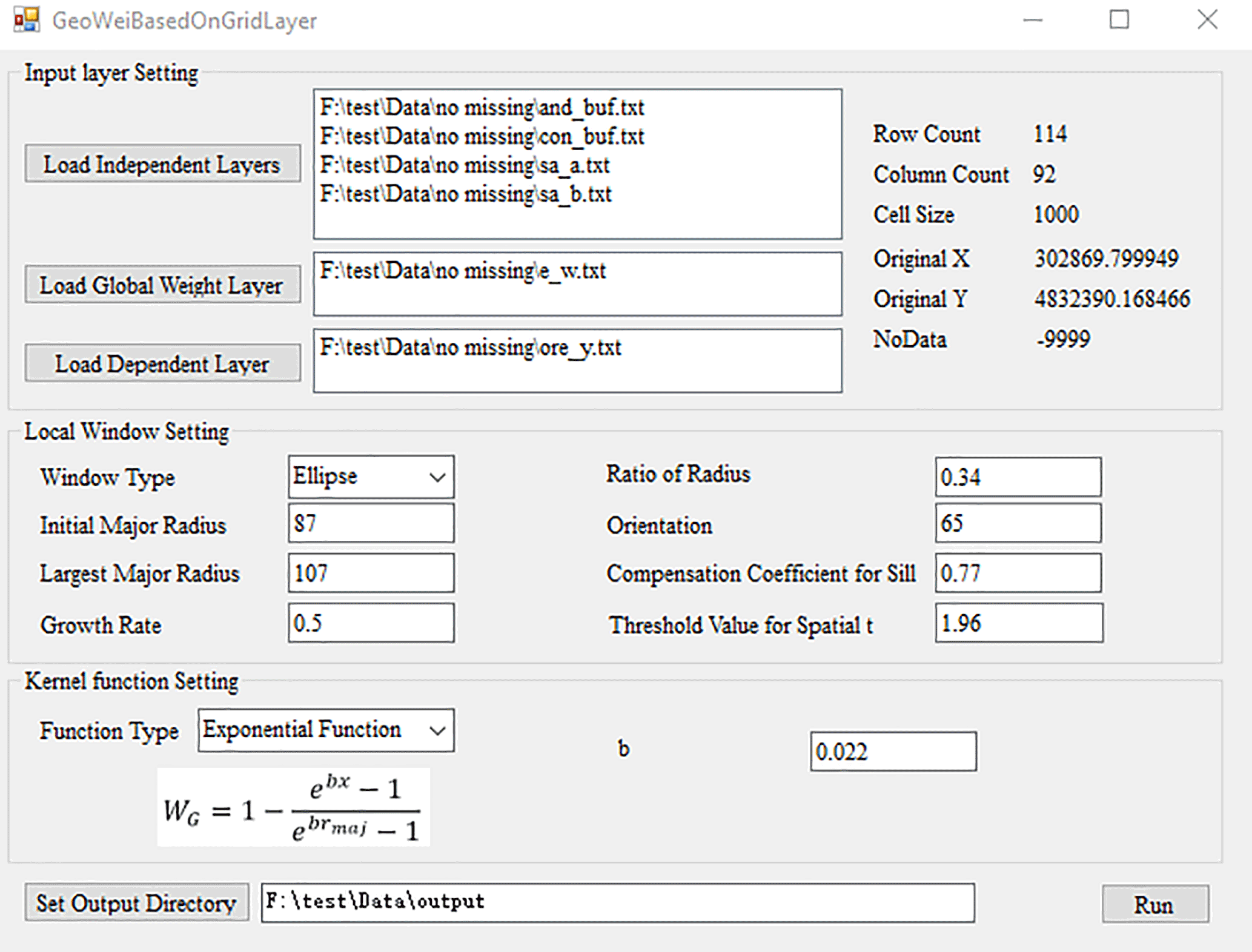
Figure 4 Evidential layers used to map Au deposits in this study: buffer of anticline axes (a), buffer for the contact of Goldenville–Halifax Formation (b), and background (c) and anomaly (d) separated with the S-A filtering method based on the ore element loadings of the first component.

• Step 1. Establish a loop for all grids in the study area according to both the columns and rows. Determine a basic local window with a size of r_min based on a variation function or other method. In addition, the maximum local window size is set as r_max, with an interval of ΔR. Suppose that a geographical weighted model has already been given in the form of a Gaussian curve determined from variations in geostatistics, i.e., $W\left(\mathrm{g}\right)={{\mathrm{e}}^{-\mathit{\lambda }d}}^{\mathrm{2}}$, where d is the distance and λ is the attenuation coefficient, then we can calculate the geographical weight for any grid in the current local window. The equivalent radius should be used in the anisotropic situation. When other types of weights are considered, e.g., the degree of exploration or research, it is also necessary to synthesize the geographical weights with other weights (see Eq. 13).

• Step 2. Establish a loop for all independent variables. In a circular (elliptical) window with a radius (equivalent radius) of r_min, apply the WofE (Agterberg, 1992) model according to the grid weight determined in step 1, thereby obtaining a statistical table containing the parameters $W_{ij}^{+}$, $W_{ij}^{-}$, and t_ij where i is the ith independent variable and j denotes the jth binarization.

• Step 2.1. If a maximum t_ij exists and it is greater than or equal to the standard t value (e.g., 1.96), record the values of $W_{i-\max \mathit{\_}t}^{+}$, $W_{i-\max \mathit{\_}t}^{-}$, and B_{i−max_t}, which denote the positive weight, negative weight, and corresponding binarization, respectively, under the condition in which t takes the maximum value. Go to step 2 and apply the WofE model to the other independent variables.

• Step 2.2. If a maximum t_ij does not exist or it is smaller than the standard t value, go to step 3.

• Step 3. In a circular (elliptical) window with a radius (equivalent radius) of r_max, increase the current local window radius from r_min according to the algorithm in step 1.

• Step 3.1. If all independent variables have already been processed, go to step 4.

• Step 3.2. If the size of the current local window exceeds the size of r_max, disregard the current independent variable and go to step 2 to consider the remaining independent variables.

• Step 3.3. Apply the WofE model according to the grid weight determined in step 1 in the current local window. If a maximum t_ij exists and it is greater than or equal to the standard t value, record the values of $W_{i-\max \mathit{\_}t}^{+}$, $W_{i-\max \mathit{\_}t}^{-}$, B_{i−max_t}, and r_current, which represent the radius (equivalent radius) for the current local window.

• Step 3.4. If a maximum t_ij does not exist or it is smaller than the standard t value, go to step 3.

• Step 4. Suppose that n_s independent variables still remain.

• Step 4.1. If n_s≤1, calculate the mean value for the dependent variable in the current local window with a radius size of r_max and retain it as the posterior probability in the current location. In addition, set the regression coefficients for all independent variables as missing data. Go to step 6.

• Step 4.2. If n_s≥1, find the independent variable with the largest local window and apply the WofE model to all other independent variables, and then update the values of $W_{i-\max \mathit{\_}t}^{+}$, $W_{i-\max \mathit{\_}t}^{-}$, and B_{i−max_t}. Go to step 5.

• Step 5. Apply the logistic regression model based on the previously determined geographic weights, and for each independent variable (1) use $W_{i-\max \mathit{\_}t}^{+}$ to replace all values that are less than or equal to B_{i−max_t}, (2) use $W_{i-\max \mathit{\_}t}^{-}$ to replace all values that are greater than B_{i−max_t}, and (3) use 0 to replace no data (“−9999”). The posterior probability and regression coefficients can then be obtained for all independent variables at the current location. Go to step 6.

• Step 6. Take the next grid as the current location and repeat steps 2–5.

4 Interface design

Before performing spatially weighted logistical regression with ILRBSWT 1.0, data preprocessing is performed using the ArcGIS 10.2 platform and GeoDAS 4.0 software. All data are originally stored in grid format, which should be transformed into ASCII files with the ArcToolbox in ArcGIS 10.2; after modeling with ILRBSWT 1.0, the resulting data will be transformed back into grid format

As shown in Fig. 3, the main interface for ILRBSWT 1.0 is composed of four parts.

The upper left part is for the layer input settings where independent variable layers, dependent variable layers, and global weight layers should be assigned. Layer information is shown at the upper right corner, including row numbers, column numbers, grid size, ordinate origin, and the expression for missing data. The local window parameters and weight attenuation function can be defined as follows. Using the drop-down list, we prepared a circle or ellipse to represent various isotropic and anisotropic spatial conditions, respectively. The corresponding window parameters should be set for each window type. For the ellipse, it is necessary to set parameters composed of the initial length of the equivalent radius (initial major radius), final length of the equivalent radius (largest major radius), increase in the length of the equivalent radius (growth rate), threshold of the spatial t value used to determine the need to enlarge the window, length ratio of the major and minor axes, orientation of the ellipse's major axis, and compensation coefficient for the sill. We prepared different types of weight attenuation functions via the drop-down menu to provide choices to users, such as exponential model, logarithmic model, Gaussian model, and spherical model, and corresponding parameters can be set when a certain model is selected. The output file is defined at the bottom and the execution button is at the lower right corner.

5 Real data testing

5.1 Data source and preprocessing

The test data used in this study were obtained from the case study reported in Cheng (2008). The study area (≈ 7780 km²) is located in western Meguma Terrain, Nova Scotia, Canada. Four independent variables were used in the WofE model for gold mineral potential mapping by Cheng (2008), i.e., buffer of anticline axes, buffer for the contact of Goldenville–Halifax Formation, and background and anomaly separated with the S-A filtering method based on ore element loadings of the first component, as shown in Fig. 4.

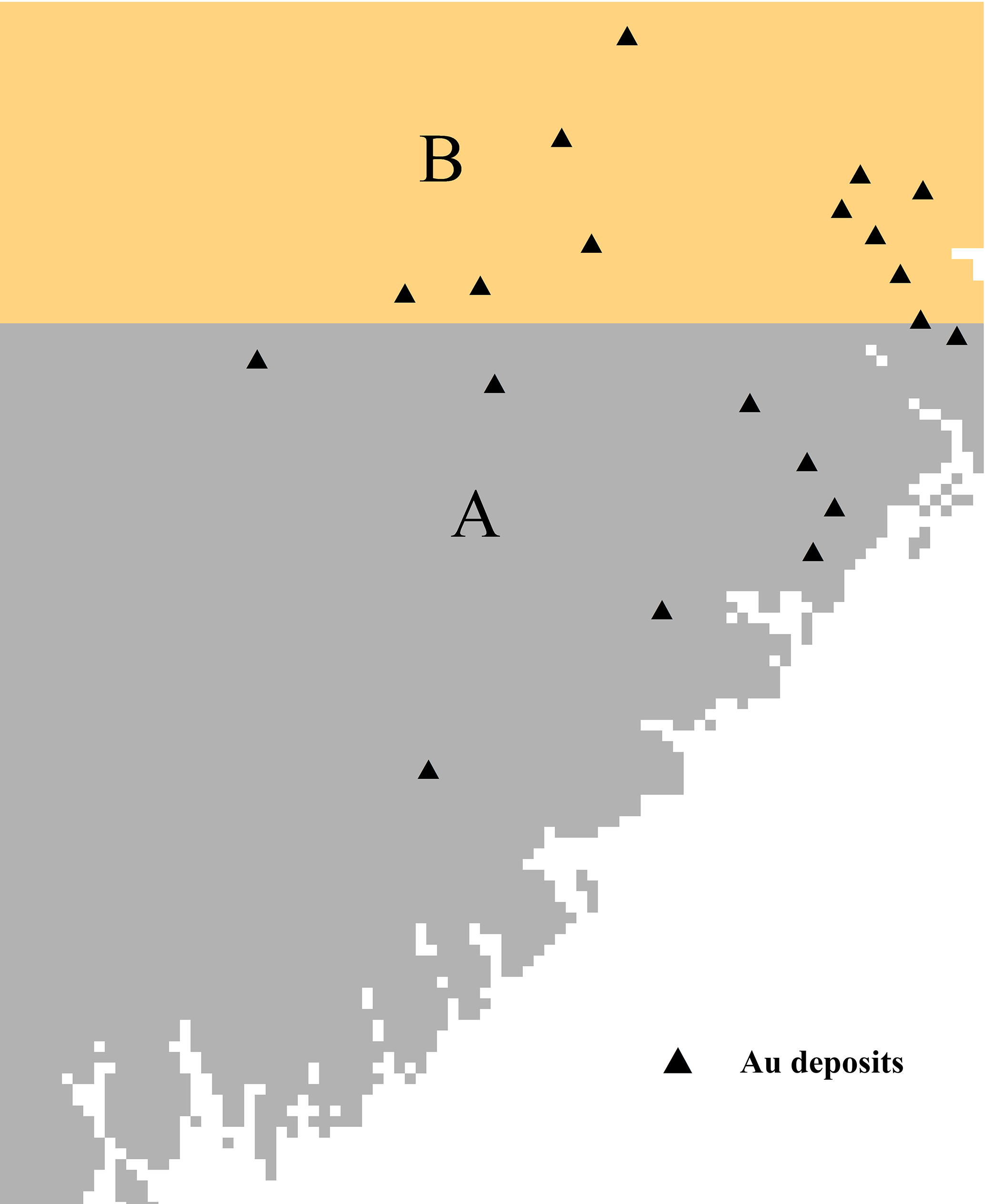
The four independent variables described previously were also used for ILRBSWT modeling in this study (see Fig. 4a to d), and they were uniformed in the ArcGIS grid format with a cell size of 1 km × 1 km. To demonstrate the advantages of the new method for missing data processing, we designed an artificial situation in Fig. 5; i.e., grids in region A have values for all four independent variables, while they only have values for two independent variables and no values in the two geochemical variables in region B.

Figure 5 Study area (A and B) where there are missing geochemical data in area B.

5.2 Mapping weights for exploration

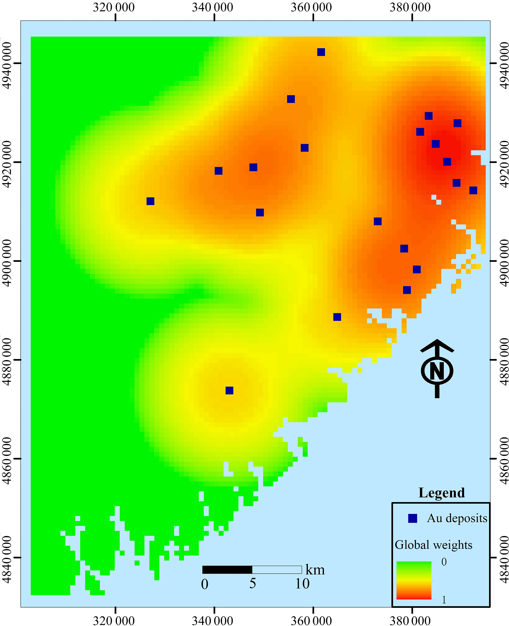
Exploration-level weights can be determined based on prior knowledge about data quality, e.g., different scales may exist throughout the whole study area; however, these weights can also be calculated quantitatively. The density of known deposits is a good index for the exploration level; i.e., the research is more comprehensive when more deposits are discovered. The exploration-level weight layer for the study area was obtained using the kernel density tool provided by the ArcToolbox in ArcGIS 10.2, as shown in Fig. 6.

Figure 6 Exploration-level weights.

5.3 Parameter assignment for local window and weight attenuation function

Both empirical and quantitative methods can be used to determine the local window parameters and attenuation function for geographical weights. The variation function in geostatistics, which is an effective method for describing the structures and trends in spatial variables, was applied in this study. To calculate the variation function for the dependent variable, it is necessary to first map the posterior probability using the global logistic regression method before determining the local window type and parameters from the variation function. Variation functions were established in four directions to detect anisotropic changes in space. If there are no significant differences among the various directions, a circular local window can be used for ILRBSWT, as shown in Fig. 1; otherwise, an elliptic local window should be used, as shown in Fig. 2. The specific parameters for the local window in the study area were obtained as shown in Fig. 7, and the final local window and geographical weight attenuation were determined as indicated in Fig. 8a and b, respectively.

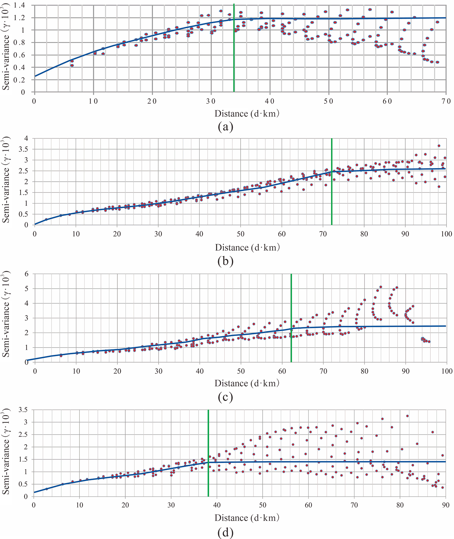
Figure 7 Experimental variogram fitting in different directions; the green lines denote the variable ranges determined for azimuths of (a) 0^∘, (b) 45^∘, (c) 90^∘, and (d) 135^∘.

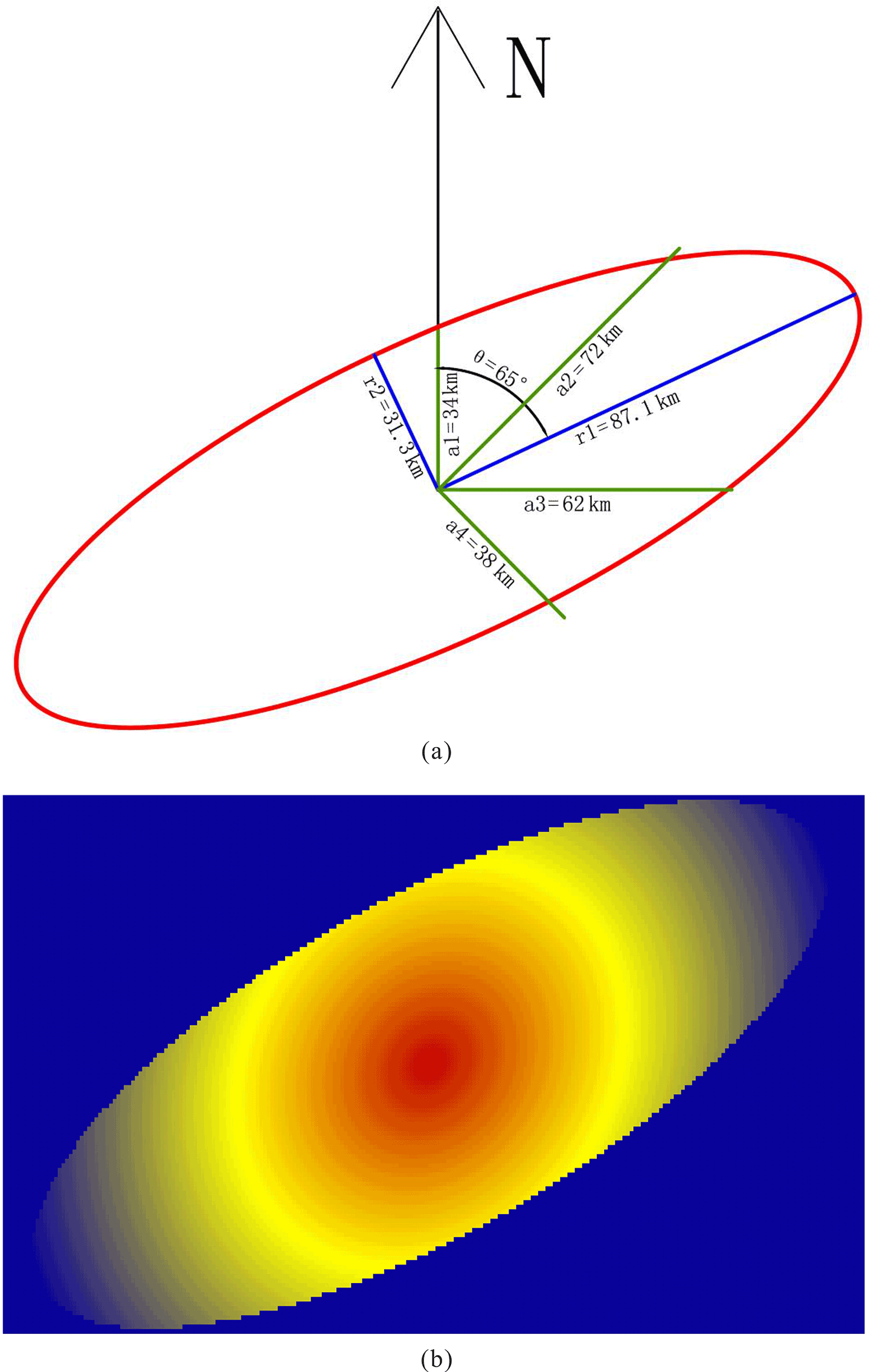
Figure 8 Nested spherical model for different directions. The green lines in (a) correspond to those in Fig. 5, and (b) shows the geographical weight template determined based on (a).

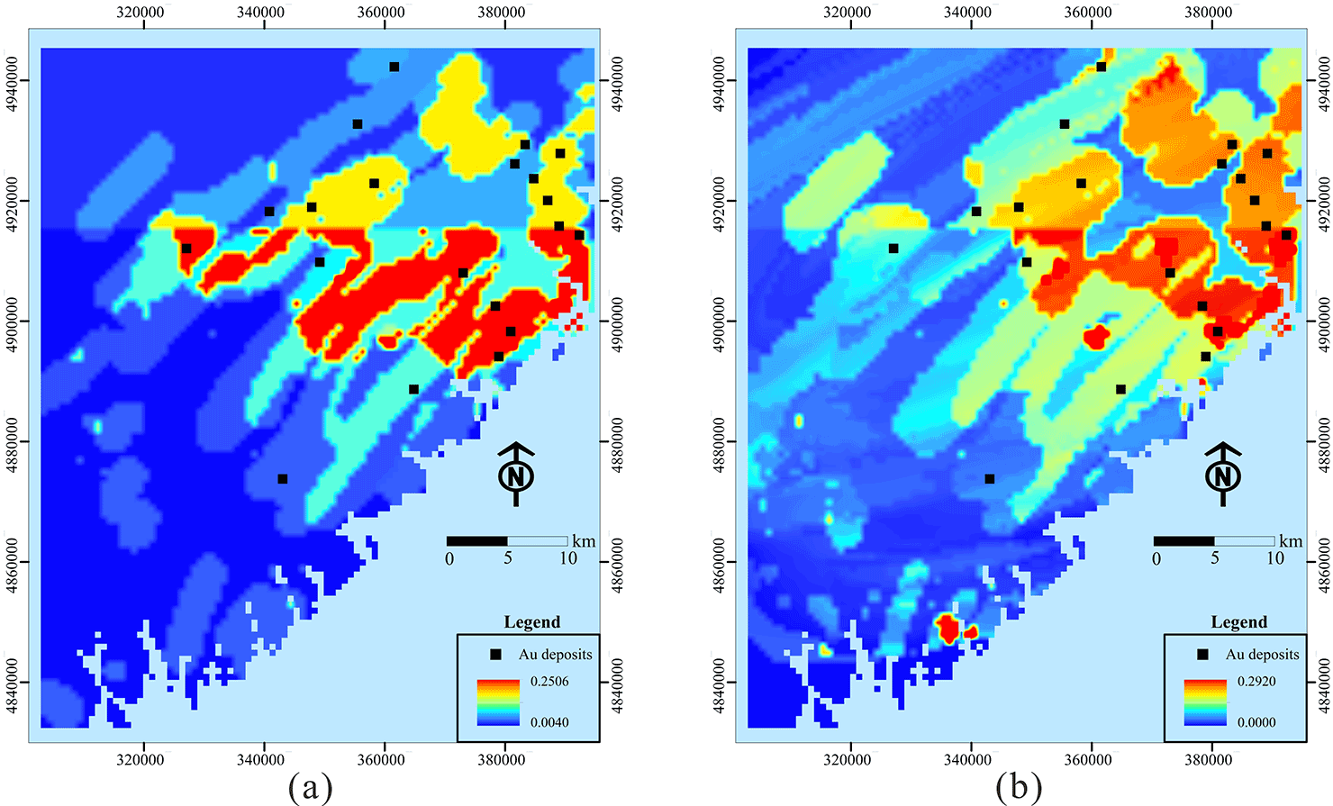
Figure 9 Posterior probability maps obtained for Au deposits by (a) logistic regression and (b) ILRBSWT.

Figure 10 Prediction–area (P-A) plots for discretized posterior probability maps obtained by logistic regression and ILRBSWT.

5.4 Data integration

Using the algorithm described in Sect. 3.2, ILRBSWT was applied to the study area according to the parameter settings in Fig. 3. The estimated probability map obtained for Au deposits by ILRBSWT is shown in Fig. 9b, while Fig. 9a presents the results obtained by logistic regression. As shown in Fig. 8, ILRBSWT better manages missing data than logistic regression, as the Au deposits in the north part of the study area (with missing data) fit better within the region with higher posterior probability in Fig. 9b than in Fig. 9a.

5.5 Comparison of the mapping results

To evaluate the predictive capacity of the newly developed and traditional methods, the posterior probability maps obtained through logistic regression and ILRBSWT shown in Fig. 9a and b were divided into 20 classes using the quantile method. Prediction–area (P-A) plots (Mihalasky and Bonham-Carter, 2001; Yousefi et al., 2012; Yousefi and Carranza, 2015a) were then made according to the spatial overlay relationships between Au deposits and the two classified posterior probability maps in Fig. 10a and b, respectively. In a P-A plot, the horizontal ordinate indicates the discretized classes of a map representing the occurrence of deposits. The vertical scales on the left and right sides indicate the percentage of correctly predicted deposits from the total known mineral occurrences and the corresponding percentage of the delineated target area from the total study area (Yousefi and Carranza, 2015a). As shown in Fig. 10a and b, with the decline of the posterior probability threshold for the mineral occurrence from left to right on the horizontal axis, more known deposits are correctly predicted, and in the meantime more areas are delimited as the target area; however, the growth in the prediction rates for deposits and corresponding occupied area is similar before the intersection point in Fig. 10a, while the former shows a higher growth rate than the latter in Fig. 10b. This difference suggests that ILRBSWT can predict more known Au deposits than logistic regression for delineating targets with the same area and indicates that the former has a higher prediction efficiency than the latter.

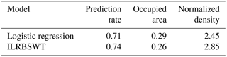
It would be a little inconvenient to consider the ratios of both predicted known deposits and occupied area. Mihalasky and Bonham-Carter (2001) proposed a normalized density, i.e., the ratio of the predicted rate of known deposits to its corresponding occupied area. The intersection point in a P-A plot is the crossing of two curves. The first is fitted from scatterplots of the class number of the posterior probability map and the rate of predicted deposit occurrences (the “prediction rate” curves in Fig. 10). The second is fitted according to the class number of the posterior probability map and corresponding accumulated area rate (the “area” curves in Fig. 10). At the interaction point, the sum of the prediction rate and corresponding occupied area rate is 1; the normalized density at this point is more commonly used to evaluate the performance of a certain spatial variable in indicating the occurrence of ore deposits (Yousefi and Carranza, 2015a). The intersection point parameters for both models are given in Table 1. As shown in the table, 71 % of the known deposits are correctly predicted with 29 % of the total study area delineated as the target area when the logistic regression is applied; if ILRBSWT if applied, 74 % of the known deposits can be correctly predicted with only 26 % of the total area delineated as the target area. The normalized densities for the posterior probability maps obtained from the logistic regression and ILRBSWT are 2.45 and 2.85, respectively; the latter performed significantly better than the former.

Table 1 Parameters extracted from the intersection points in Fig. 10a and b.

6 Discussion

Because of potential spatial heterogeneity, the model parameter estimates obtained based on the total equal-weight samples in the classical regression model may be biased, and they may not be applicable for predicting each local region. Therefore, it is necessary to adopt a local window model to overcome this issue. The presented case study shows that ILRBSWT can obtain better prediction results than classical logistic regression because of the former's sliding local window model, and their corresponding intersection point values are 2.85 and 2.45, respectively. However, ILRBSWT has advantages. For example, characterizing 26 or 29 % of the total study area as a promising prospecting target is too high in terms of economic considerations. If instead 10 % of the total area is mapped as the target area, the proportions of correctly predicted known deposits obtained by ILRBSWT and logistic regression are 44 and 24 %, respectively. The prediction efficiency of the former is 1.8 times larger than the latter.

In this study, we did not separately consider the influences of spatial heterogeneity, missing data, and degree of exploration weight, so we cannot evaluate the impact of each factor. Instead, the main goal of this work was to provide the ILRBSWT tool, thereby demonstrating its practicality and overall effect. Zhang et al. (2017) applied this model to mapping intermediate and felsic igneous rocks and proved the effectiveness of the ILRBSWT tool in overcoming the influence of spatial heterogeneity specifically. In addition, Agterberg and Bonham-Carter (1999) showed that WofE has the advantage of managing missing data, and we have taken a similar strategy in ILRBSWT. We did not fully demonstrate the necessity of using exploration weight in this work, which will be a direction for future research. However, it will have little influence on the description and application of the ILRBSWT tool as it is not an obligatory factor, and users can individually decide if the exploration weight should be used.

Similar to WofE and logistic regression, ILRBSWT is a data-driven method, and thus it inevitably suffers from the same problems as data-driven methods, e.g., the information loss caused by data discretization and exploration bias caused by the training sample location. However, it should be noted that evidential layers are discretized in each local window instead of the total study area, which may cause less information loss. This can also be regarded as an advantage of the ILRBSWT tool. With respect to logistic regression and WofE, some researchers have proposed solutions to avoid the information loss resulting from spatial data discretization by performing continuous weighting (Pu et al., 2008; Yousefi and Carranza, 2015b, c), and these concepts can be incorporated into further improvements of the ILRBSWT tool in the future.

7 Conclusions

Given the problems in existing MPM models, this research provides an ILRBSWT tool. We have proven its operability and effectiveness through a case study. This research is also expected to provide software tool support for geological exploration researchers and workers in overcoming the nonstationarity of spatial variables, missing data, and differences in exploration degree, which should improve the efficiency of MPM work.