the Creative Commons Attribution 4.0 License.
the Creative Commons Attribution 4.0 License.
 | 22 Jun 2018
A conservative reconstruction scheme for the interpolation of extensive quantities in the Lagrangian particle dispersion model FLEXPART
Sabine Hittmeir
Anne Philipp
Petra Seibert
Lagrangian particle dispersion models require interpolation of all meteorological input variables to the position in space and time of computational particles. The widely used model FLEXPART uses linear interpolation for this purpose, implying that the discrete input fields contain point values. As this is not the case for precipitation (and other fluxes) which represent cell averages or integrals, a preprocessing scheme is applied which ensures the conservation of the integral quantity with the linear interpolation in FLEXPART, at least for the temporal dimension. However, this mass conservation is not ensured per grid cell, and the scheme thus has undesirable properties such as temporal smoothing of the precipitation rates. Therefore, a new reconstruction algorithm was developed, in two variants. It introduces additional supporting grid points in each time interval and is to be used with a piecewise linear interpolation to reconstruct the precipitation time series in FLEXPART. It fulfils the desired requirements by preserving the integral precipitation in each time interval, guaranteeing continuity at interval boundaries, and maintaining non-negativity. The function values of the reconstruction algorithm at the sub-grid and boundary grid points constitute the degrees of freedom, which can be prescribed in various ways. With the requirements mentioned it was possible to derive a suitable piecewise linear reconstruction. To improve the monotonicity behaviour, two versions of a filter were also developed that form a part of the final algorithm. Currently, the algorithm is meant primarily for the temporal dimension. It was shown to significantly improve the reconstruction of hourly precipitation time series from 3-hourly input data. Preliminary considerations for the extension to additional dimensions are also included as well as suggestions for a range of possible applications beyond the case of precipitation in a Lagrangian particle model.
- Article
(7797 KB) - Full-text XML
-
Supplement
(140 KB) - BibTeX
- EndNote


In numerical models, extensive variables (those being proportional to the volume or area that they represent, e.g. mass and energy) are usually discretised as grid-cell integral values so that conservation properties can be fulfilled. A typical example is the precipitation flux in a meteorological forecasting model. Usually, one is interested in the precipitation at the surface, and thus the quantity of interest is a two-dimensional horizontal integral (coordinates x and y) over each grid cell. Furthermore, it is accumulated over time t during the model run and written out at distinct intervals together with other variables, such as wind and temperature. After the trivial postprocessing step of de-accumulation, each value thus represents an integral in x, y, t space – the total amount of precipitation which fell on a discrete grid cell during a discrete time interval.
In Lagrangian particle dispersion models (LPDMs) (Lin et al., 2013), it is necessary to interpolate the field variables obtained from a meteorological model to particle positions in (three-dimensional) space and in time. The simplest option, to assign the value corresponding to the grid cell in which the particle resides (often called “nearest-neighbour” method), is not sufficiently accurate. For example, in the case of precipitation, this would lead to an unrealistic, checkerboard-like deposition field. A simple approach for improvement would be to ascribe the gridded precipitation value to the spatio-temporal centre of the space–time cell and then perform linear interpolation between these points, as illustrated in Fig. 1. While this works for the case of intensive field quantities (velocity, temperature, etc.) where gridded data truly represent point values, it is not a satisfactory solution for extensive quantities, as it does not conserve the total amount in each time interval, as will be shown below. The problem became obvious to us with respect to the precipitation field in the LPDM FLEXPART (Stohl et al., 2005). Therefore, it will be discussed using this example, even though the problem is of a general nature and the solution proposed has a wide range of possible applications.
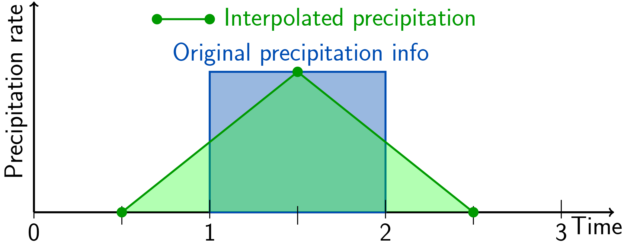
Figure 1Illustration of the basic problem using an isolated precipitation event lasting one time interval represented by the thick blue line. The amount of precipitation is given by the blue-shaded area. Simple discretisation would use the green circles as discrete grid-point representation and interpolate linearly in between, indicated by the green line and the green-shaded area. Note that supporting points for the interpolation are shifted by a half-time interval compared to the times when other meteorological fields are available.
1.1 Introduction of the problem using the example of precipitation in FLEXPART
FLEXPART is a LPDM, which is typically applied to study air pollution but is also used for other problems requiring the quantification of atmospheric transport, such as the global water cycle or the exchange between the stratosphere and the troposphere; see Stohl et al. (2005). Before a FLEXPART simulation can be done, a separate preprocessor is used to extract the meteorological input data from the Meteorological Archival and Retrieval System (MARS) of the European Centre for Medium Range Weather Forecasts (ECMWF) and prepare them for use in the model.1 The model is also able to ingest meteorological fields from the United States National Center for Environmental Prediction. However, it was originally designed for ECMWF fields, and we limit our discussion here to this case. Currently, a relatively simple method processes the precipitation fields in a way that is consistent with the scheme applied in FLEXPART for all variables: linear interpolation between times where input fields are available. Under these conditions, it is not possible to conserve the original amount of precipitation in each grid cell. The best option, which was realised in the preprocessing, is conservation within the interval under consideration plus the two adjacent ones. Unfortunately, this leads to undesired temporal smoothing of the precipitation time series – maxima are damped and minima are raised. It is even possible to produce non-zero precipitation in dry intervals bordering a precipitation period as shown in Fig. 2. This is obviously undesirable as it will affect wet scavenging, a very efficient removal process for many atmospheric trace species. Wet deposition may be produced in grid cells where none should occur, or too little may be produced in others. Different versions of the FLEXPART data extraction software refer to this process as “disaggregation” or “de-accumulation”.
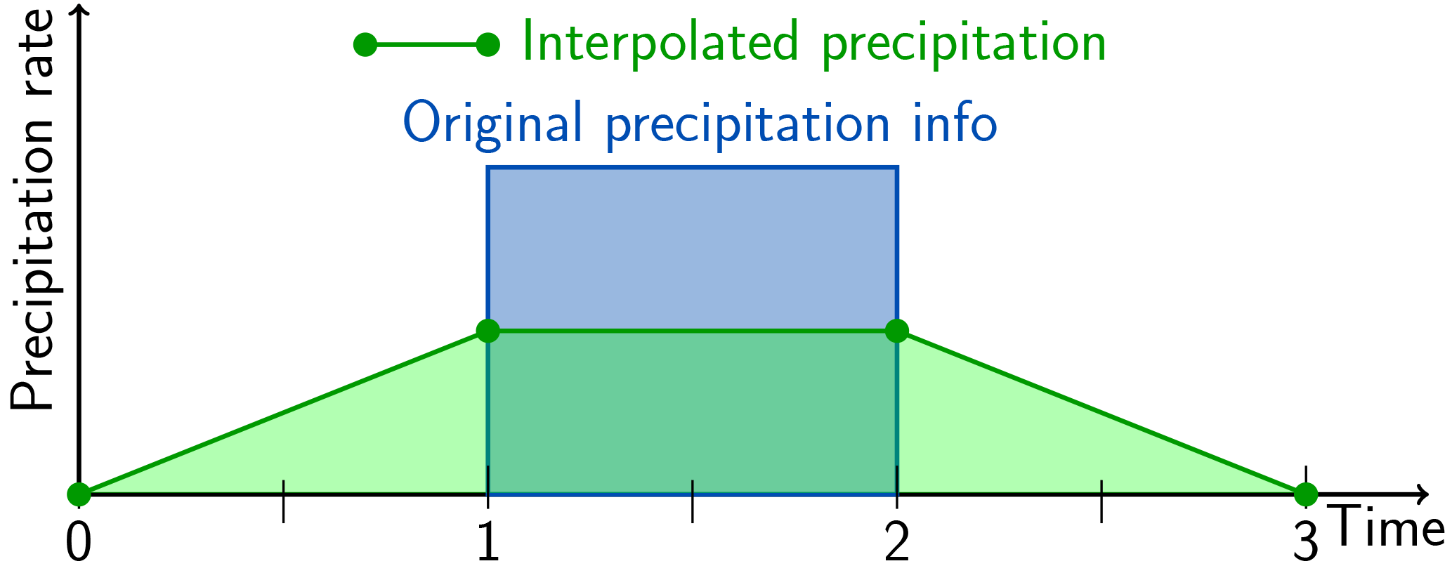
Figure 2Example of so-called “disaggregation” of precipitation data for the use in FLEXPART as currently implemented, with the case of an isolated precipitation period. Note that the supporting points for the interpolation now coincide with the times when other meteorological fields are available. Colours are used as in Fig. 1.
Horizontally, the precipitation values are averages for a grid cell around the grid point to which they are ascribed, and FLEXPART uses bilinear interpolation to obtain precipitation rates at particle positions. This causes the same problem of spreading out the information to the neighbouring grid cells and implied smoothing.2 However, the supporting points in space are not shifted between precipitation and other variables as is the case for the temporal dimension.
The goal of this work is to develop a reconstruction algorithm for the one-dimensional temporal setting which
-
strictly conserves the amount of precipitation within each single time interval,
-
preserves the non-negativity,
-
is continuous at the interval borders,
-
and ideally also should reflect a natural precipitation curve (this latter condition can be understood in the sense that the reconstruction graph should possess good monotonicity properties),
-
should be efficient and easy to implement within the existing framework of the FLEXPART code and its data extraction preprocessor.
These requirements on the reconstruction algorithm imply that time intervals with no precipitation remain unchanged, i.e. the reconstructed values vanish throughout this whole time interval, too. In the simplest scenario of an isolated precipitation event, where in the time interval before and after the data values are zero, the reconstruction algorithm therefore has to vanish at the boundaries of the interval, too. The additional conditions of continuity and conservation of the precipitation amount then require us to introduce sub-grid points if we want to keep a linear interpolation (Fig. 3). The height is thereby determined by the condition of conservation of the integral of the function over the time interval. The motivation for a linear formulation arises from the last point of the above list of desirable properties.

Figure 3Precipitation rate linearly interpolated using a sub-grid with two additional points. Colours as in Fig. 1.
It can be noted that in principle a single sub-grid point per time interval would be sufficient. This, however, would result in very high function values and steep slopes of the reconstructed curve, which appears to be less realistic and thus not desirable.
As we shall see in the next section, closing the algorithm for such isolated precipitation events is quite straightforward, since the only degree of freedom constituting the height of the reconstruction function is determined by the amount of precipitation in the interval. However, the situation becomes much more involved if longer periods of precipitation occur, i.e. several consecutive time intervals with positive data. Then, in general, each sub-grid function value constitutes 1 degree of freedom (Fig. 4).

Figure 4Illustration of a reconstruction for longer periods with positive data values, where each sub-grid function value constitutes 1 degree of freedom.
Therefore, in order to close the algorithm, we have to fix all of these additionally arising degrees of freedom. As a first step we make a choice for the slope in the central subinterval, which relates the two inner sub-grid function values. Three possible approaches are discussed for this choice. Conservation provides a second condition. These two can be considered to determine the two inner sub-grid points. Then, the function values at the grid points in between time intervals of positive data are left to be prescribed, and as each point belongs to two intervals, this corresponds to the third degree of freedom. The steps leading to the final algorithm (of which there are some variants) are presented in Sect. 3. Ways for extending the one-dimensional algorithms to a two-dimensional setting are briefly discussed as well. Note that we use the wording “reconstruction algorithm” and “interpolation algorithm” interchangeably.
In the following Sect. 2, some existing literature on conservative reconstruction algorithms is briefly reviewed, with an emphasis on applications used for semi-Lagrangian advection schemes in Eulerian models. To our knowledge, confirmed by contacts with people active in this field, a piecewise linear, conservative reconstruction algorithm using a sub-grid has not yet been proposed.
Section 4 then presents an evaluation of the algorithms by verifying them with synthetic data and validating them with original data from ECMWF where the available 1-hourly resolution serves as a reference data set and the 3-hourly resolution as input for the interpolation algorithms. The verification demonstrates that the demanded requirements are indeed fulfilled, and the validation compares the accuracy of the new algorithms with the one currently used to show the improvements.
The conclusions (Sect. 5) summarise the findings, present an outlook for the next steps, and suggest a range of possible applications of the new reconstruction algorithm beyond the narrow case of precipitation input to a Lagrangian particle dispersion model.
A widely used form of interpolation is the well-known spline interpolation consisting of piecewise polynomials, which are typically chosen as cubic ones (e.g. Hämmerlin and Hoffmann, 1994; Hermann, 2011). The task of finding an appropriate piecewise polynomial interpolation, which is non-negative, continuous, mass conserving, and monotonic is a challenging one. This fact has also been pointed out by White et al. (2009), who stated that building a reconstruction profile satisfying all these requirements is generally not possible. Typically, the reconstruction profiles are not continuous on the edges of the grid cells. Sufficient conditions for positive spline interpolation in form of inequalities on the interpolation's coefficients have been derived in Schmidt and Heß (1988).
The issue of mass-conservative interpolation emerges also in the context of semi-Lagrangian finite-volume advection schemes, which have become very popular. These schemes, with a two-dimensional application in mind, are known under the heading of “remapping”. Eulerian grid cells are mapped to the respective areas covered in the previous time step, and then the mass in this area is calculated by a reconstruction function from the available grid-cell average values (Lauritzen et al., 2010). Apart from global interpolation functions such as Fourier methods, piecewise defined polynomials are the method of choice in this context. They can be piecewise constant, linear, parabolic (second-order), or cubic (third-order). The first two options are usually discarded as not being accurate enough. While this application shares the need for the reconstruction to be conservative and positively definite and the aim of preserving monotonicity, with our problem there are some aspects where the characteristics of the problems are different. For the advection schemes, continuity at the cell interface is not a strict condition. However, they need to be able to reconstruct sharp peaks inside each volume, as otherwise through the repetitive application during the numerical integrations, strong artificial smoothing of sharp structures would result. Therefore, at least second-order and if possible higher-order methods are preferred. The drawback of higher-order reconstruction functions is their tendency to overshoot and produce wiggles, which have to be removed or reduced by some sort of filter. However, as in the remapping process one always integrates over some domain, this is less of an issue than in our case, where for each computational particle we need an interpolated value at exactly one point.
An interesting example of such a semi-Lagrangian conservative remapping is given by Zerroukat et al. (2002). The coefficients of the one-dimensional cubic spline in each interval are determined using the conservation of mass in the underlying interval. The function values at the left border points are determined by an additional spline interpolation using the condition of mass conservation in the two preceding, the current, and the following intervals. The function values at the right border points are determined in a similar fashion. This construction in particular provides continuity. A monotonic and positively definite filter has then been applied to this semi-Lagrangian scheme (Zerroukat et al., 2005), which first detects regions of non-monotonic behaviour and then locally reduces the order of the polynomial until monotonicity is regained. An improved version of this filter without reducing the order of the interpolating polynomial in most cases is provided in Zerroukat et al. (2006), where a parabolic spline is used for interpolation. The basic algorithm in all these cases is one-dimensional, where the application to the two-dimensional case has been explicitly demonstrated only in Zerroukat et al. (2005), as a combination of the so-called cascade splitting and the one-dimensional algorithm.
Considering the differences mentioned between the reconstruction problem arising in the context of semi-Lagrangian advection schemes and of the LPDM FLEXPART and the fact that in addition that linear interpolation is used in FLEXPART for all other quantities and that evaluation of the interpolation function has to be done efficiently for up to millions of particles in each time step, we have chosen to construct a non-negative, continuous, and conservative reconstruction algorithm based upon piecewise linear interpolation. Contrary to standard piecewise linear methods, we divide each grid interval into three subintervals, so that our method has some similarity with a piecewise parabolic approach while being simpler and presumably faster.
3.1 Notation and basic requirements
In accordance with the considerations presented in Sect. 1, we consider our input data to be precipitation values defined over a period [0, T], where T is the time at the end of the period. They are available as amounts (or equivalently, as average precipitation rates) during N−1 constant time intervals of duration Δt, bounded by equidistant times ti where
The time intervals for which the precipitation amounts are defined are denoted as
The precipitation rate is then represented as a step function with values
As an abbreviation, we write g(0)=g0. The total precipitation within one time interval Ii is then given by
Our aim is to find a piecewise linear function to serve as interpolation. We require it
-
to be continuous,
-
to preserve the non-negativity such that f satisfies
-
to conserve the precipitation amount within each single time interval Ii, i.e.
in particular,
These conditions are also listed in Table 2 as the three strict and main requirements of the algorithm. They necessitate the introduction of sub-grid points. A single sub-grid point was deemed insufficient for a realistic representation of precipitation time series. For simplicity, we choose an equidistant sub-grid setting with two additional points:
The subintervals resulting from these sub-grid points are defined as , , , and the slopes of the interpolation algorithm f in these subintervals are denoted accordingly by , , . The sub-grid function values are abbreviated in the following as fi:=f(ti), , . Figure 5 shows a schematic overview of these definitions.
It is evident that the function f in Ii is uniquely determined by the function values fi, , , fi+1, with linear interpolation between them. Equivalently, the problem can be stated in terms of the slopes, such that the function f in Ii is determined uniquely by fi, , , . This equivalence is based upon the relations between slopes and function values:
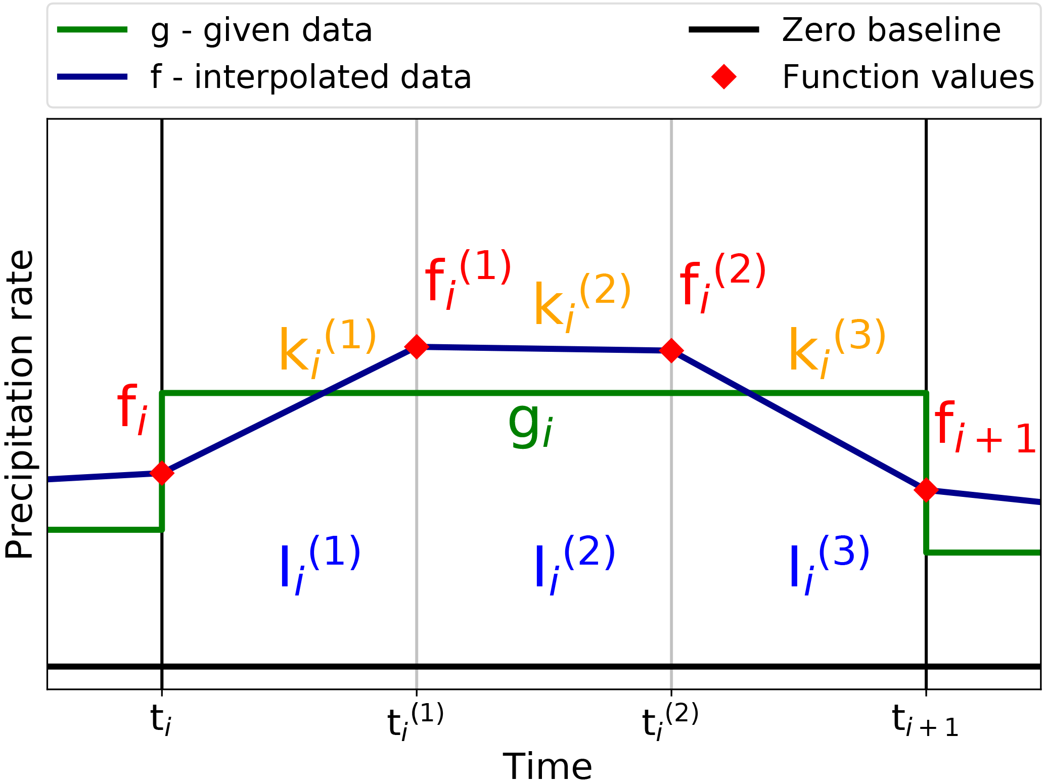
Figure 5Schematic overview of the basic notation in a precipitation interval with the original precipitation rate g (green) as a step function and the interpolated data f (dark blue) as the piecewise linear function. The original time interval with fixed grid length Δt is split equidistantly in three subintervals denoted by , with the slopes in the subintervals as denoted by . The sub-grid function values fi, , fi+1 are marked by red diamonds.
The key requirement for the interpolation algorithm f is to preserve the precipitation amount within each single time interval Ii as specified in Eq. (6). Therefore,
or, equivalently, equal areas underneath function graphs of f and g. In the following, we thus also refer to Eq. (10) as the equal-area condition. In terms of the function values, Eq. (10) amounts (after division by Δt) to
In order to fulfil Eq. (5) (non-negativity), we need a solution satisfying
As already mentioned above, a further consequence of the equal-area condition and the continuity condition is, in particular,
such that periods with zero precipitation rate remain unchanged.
3.2 Isolated precipitation in a single time interval
We first demonstrate the basic idea of the interpolation algorithm for the simplest case of an isolated precipitation event; i.e. we assume an interval i∈ℐ with gi>0 and (see Fig. 6). As Eq. (13) then holds in the surrounding intervals Ii−1 and Ii+1, the continuity condition yields at the boundary of the interval. Moreover, as we do not want to create artificial asymmetry in the problem, we let f be constant in the centred subinterval , such that the only function value left to be determined is which thus constitutes the only degree of freedom in the problem. This height of the interpolation function is now obtained via the equal-area condition Eq. (11), which in this particular case amounts to
therewith closing the algorithm.
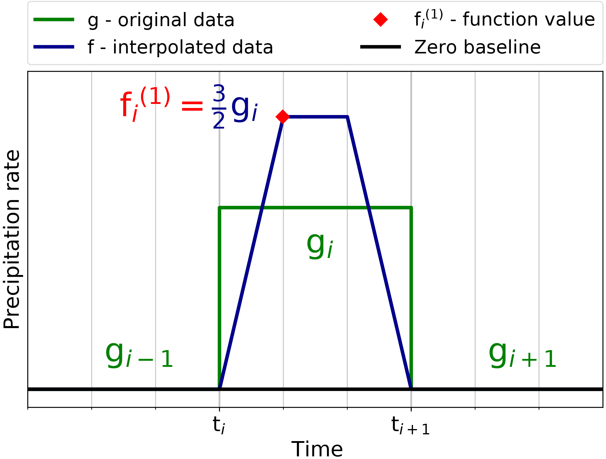
Figure 6Isolated precipitation event (no precipitation in gi−1 and gi+1). The only degree of freedom is given by the function value and is marked by a red square.
3.3 General case
Whereas the derivation of the algorithm for the isolated precipitation event is straightforward, the problem becomes considerably more involved if consecutive intervals with non-zero precipitation occur. Treating each interval as an isolated precipitation event as demonstrated in Fig. 6 by forcing the function values at the original grid points to vanish would be possible, but such an algorithm is not acceptable, as the interpolation function f has to reflect the actual course of precipitation in a realistic way. All function values fi in between periods with non-zero precipitation should be positive, too. Thus, they constitute additional degrees of freedom and need to be determined. The main challenge for a suitable interpolation algorithm lies in finding a proper way to deal with these additional degrees of freedom.
Therefore, we now consider the case of two consecutive intervals with non-zero data for some i∈ℐ. The first function value fi is assumed to be given by the algorithm in the preceding interval Ii−1 or – for the first interval – a prescribed boundary value. Then, since , we neither have the condition of vanishing fi+1, nor is the symmetry relation desirable generally. Thus, with given fi, in general there are the three degrees of freedom , , fi+1, associated with the interval Ii, as illustrated in Fig. 4. Since the equal-area condition corresponds to only one of them, two additional relations are required.
3.3.1 Boundary conditions
In the following, we assume the boundary values
as being prescribed. If their values are not explicitly provided, a simple assumption is to consider the precipitation rate to be constant in time and thus f(0)=g(0) and f(T)=g(T) or, equivalently, f0=g0 and .
3.3.2 Prescribing the central slope
As a means to reflect the actual course of precipitation, a natural first step is to prescribe the central slope . We choose it as the average of the slopes in the outer two subintervals, i.e.
which has the desirable property that it allows for the particular case . Moreover, inserting Eq. (9), we obtain the equivalent expression
This result is quite intuitive in the sense that it corresponds to the mean slope of the interpolation function throughout the interval Ii. Letting being determined via Eq. (17), the function values are uniquely determined by through Eq. (9) as
and thus the degrees of freedom are reduced accordingly.
Other possible approaches for the central slope which have not been selected would be the following:
- i.
Setting , which is the simplest choice for . It was used for the isolated precipitation event. This means that f is constant in the central subintervals , and thus . This choice, however, does not reflect a natural precipitation curve.
- ii.
A more advanced, data-driven approach would be to represent the tendency of the surrounding data values by the centred finite difference
The problem here is to fulfil the condition of non-negativity if gi is small compared to one of its neighbouring values.
3.3.3 Using the equal-area condition
Now, the function values are determined in a way that the equal-area condition in Eq. (11) is satisfied, which, after inserting Eq. (18) yields
We thus obtain for the sub-grid function values
3.3.4 Closing the algorithm under the condition of non-negativity
Equations (21) and (22) show that the algorithm is closed once the function values at the grid points fi+1 are determined. Thus, the function values fi+1 for indices i∈ℐ with still need to be determined. An obvious first choice would be to use the arithmetic mean value of the surrounding data values gi and gi+1. However, in order to fulfil Eq. (13), a case distinction is required to deal separately with and for a given gi>0. This would lead to a lack of continuity between the cases of precipitation equal to or only close to zero. For the latter case, the algorithm would even produce negative values. Therefore, the arithmetic mean is not a good choice. A better choice is the geometric mean
which has the main advantage that the case distinction is not required. With the additional Eq. (23) for the function value fi+1, having Eqs. (21) and (22) for the sub-grid values and , respectively, the algorithm is now closed. However, the problem of negative values still can arise in the case of small values in between larger ones. This is due to the fact that for , the geometric mean converges to 0 in general too slowly.
A further possible approach would be to assign with , which fulfils the non-negativity but gives a non-monotonic solution curve and thus does not produce a natural precipitation curve. A less restrictive approach would be to use . However, this would also lead to one slope being artificially set to zero, and it would thus be incompatible with a realistic course of the precipitation. Furthermore, this solution would be implicit, as the interval Ii depends on the solution in Ii+1. Since the relation is via a minimum function, one would have to distinguish between all possible cases of function values in the whole interval of precipitation, probably too complex an operation for longer periods.
We shall note that instead of prescribing the function values at the grid points directly, there are also other possible approaches. Two of them have been looked at and are discussed in the following paragraphs.
Instead of a function value, we might prescribe an additional slope. We tested a basic finite difference approach in terms of the involved data values as well as a symmetric version of it. As this does not preseve monotonicity, we also derived a global algorithm, where the slope of the right subinterval in Ii is equal to the slope in the left subinterval of the next time interval. Thus, the solution in the time interval Ii depends on the solution in the next time interval Ii+1, such that the algorithm cannot be solved for each time interval individually anymore but has to be solved globally in form of a linear system. This algorithm was shown to create better monotonicity properties, but the implementation is much more complicated and solving the problem is clearly computationally much more expensive. All of these algorithms, however, have a common fault, namely the violation of non-negativity. This is caused by the fact that the algorithms with prescribed slopes all rely on a case distinction, whether one involved precipitation value is positive or not, and therefore are not continuous with respect to vanishing values. One should also note that algorithms based on prescribing additionally the slopes for are not invariant with respect to being solved forward or backward in time. This results from the asymmetry of the slopes, since when solving backwards in time, the roles of the slopes and from the original problem are interchanged.
Another approach would be to formulate the reconstruction problem as an optimisation problem. However, for large data sets this turned out to be much more expensive than the ad hoc methods described before (using the MATLAB Optimisation Toolbox). As the final aim is to solve the interpolation problem for large data sets in three dimensions, this approach was not further studied.
The preservation of non-negativity is a challenging requirement, as discussed above. In the following, we investigate sufficient conditions for the non-negativity to hold. The algorithm consisting of Eqs. (21), (22), and (23) (function values fi+1 determined via the geometric mean) is considered as the base. It has the strong advantage of not requiring a case distinction between vanishing and positive values. It will be combined with the minimum value approach, which guarantees the non-negativity of the solutions. We thus now investigate which conditions on generally prescribed non-negative function values fi are required to guarantee that the sub-grid function values are also non-negative, i.e. . For the central slope being defined as the mean Eq. (17), the sub-grid function values are given by Eqs. (21) and (22). The requirement of non-negativity of and then amounts to
Thus, a sufficient condition for the algorithm to preserve non-negativity is the restriction
The same condition for non-negativity is obtained if the central slope is prescribed as zero, (option i in Sect. 3.3.2). With the data-driven definition of Eq. (19) for the central slope, option ii, the additional restriction
would have to be fulfilled by the input data. However, this relation is often violated in realistic precipitation data, which justifies the decision to discard this approach.
We thus return to the geometric-mean method (Eq. 23) and combine it with the non-negativity constraint Eq. (25), which results in
We have thus obtained a piecewise linear interpolation function determined by Eqs. (27), (21) and (22), which defines a non-negative, continuous, and area-preserving algorithm, called Interpolation Algorithm 0 (IA0) henceforth.
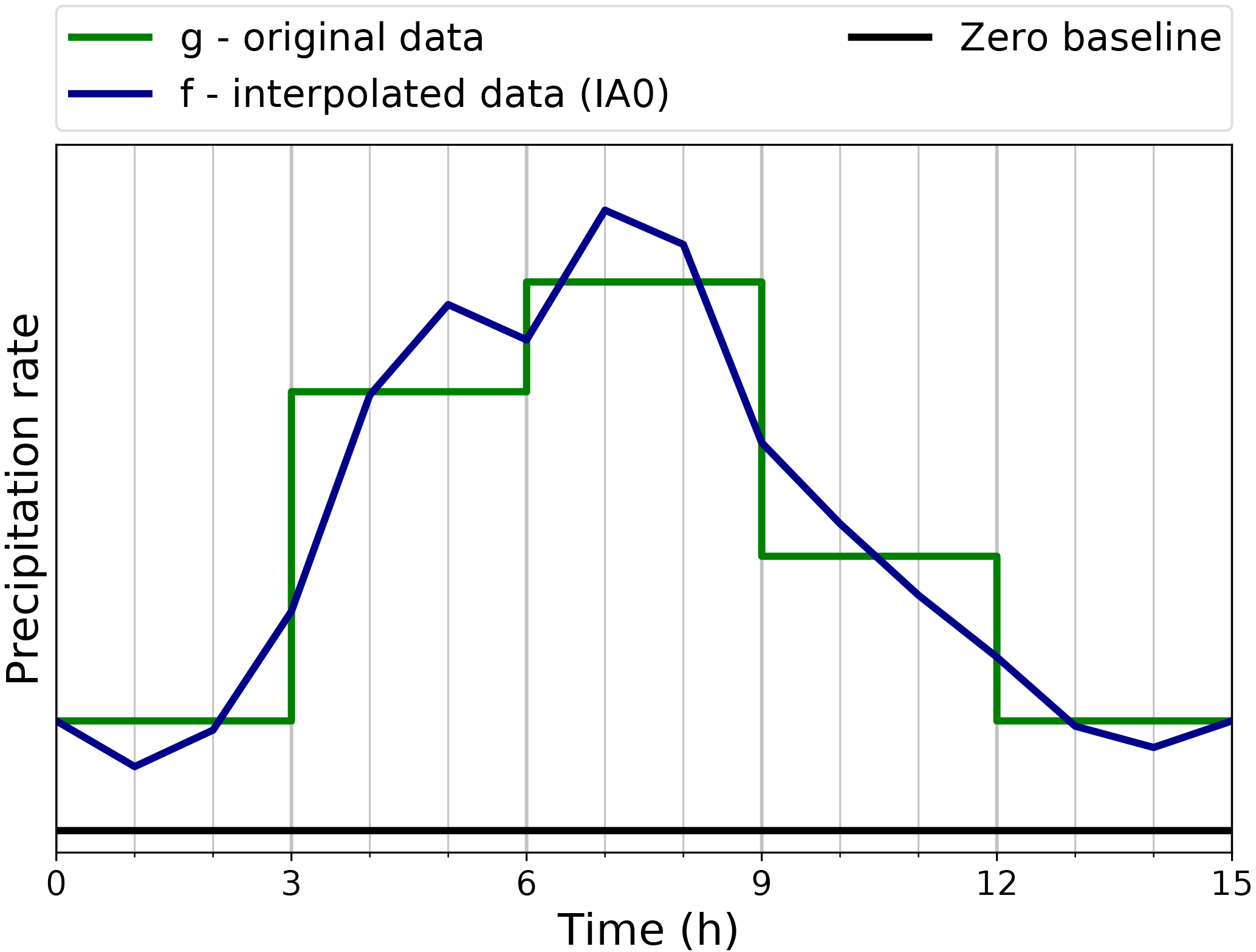
Figure 7Results with the IA0 algorithm. The original precipitation rate g is shown in green with a 3-hourly resolution. The IA0 interpolated data f on the new sub-grid with 1-hourly resolution is given in dark blue. A zero baseline is shown in black.
3.3.5 Monotonicity filter as a postprocessing step
Figure 7 illustrates the IA0 algorithm with a practical example. It fulfils the mentioned requirements, but it appears not to be sufficiently realistic, as it does not preserve the monotonicity as present in the input data (minimum at t=6 h).
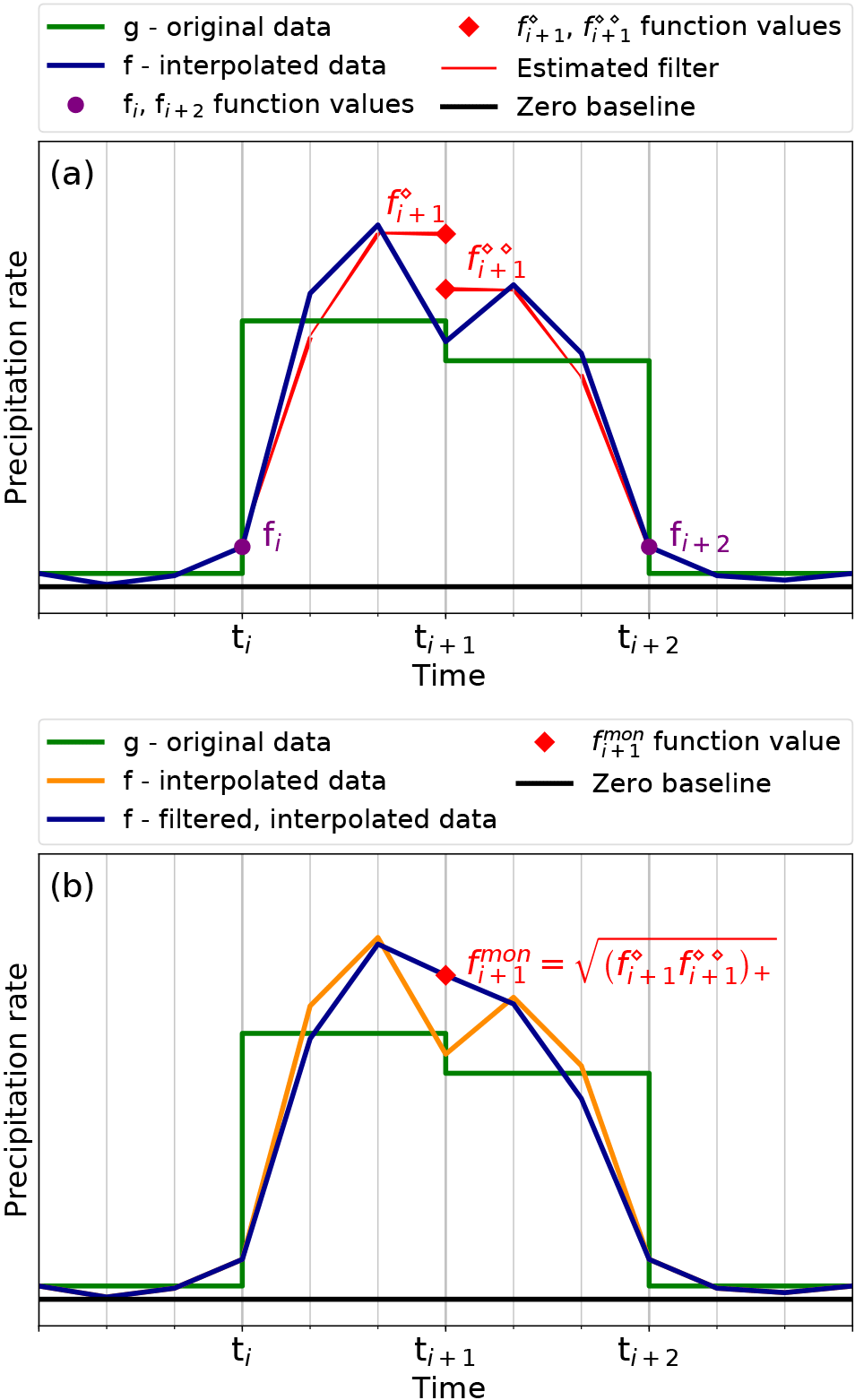
Figure 8Illustration of the monotonicity filter construction. The original precipitation rate g is shown in green with a 3-hourly resolution. A zero baseline is shown in black. (a) The interpolated series f from IA0, using the new sub-grid with 1-hourly resolution, is given in dark blue. First, the function value fi+1 is split in and shown as red squares. Other function values are recomputed as shown with the red line where fi and fi+2 remain unchanged as shown with purple circles. (b) Second, the function value fi+1 is substituted by the new function value as marked with a red square. The unfiltered graph f derived by IA0 is shown in orange here, while the filtered graph resulting after recomputation of the neighbouring values is shown in dark blue.
In response to this problem, we introduce a monotonicity filter which is active only in the regions where the graph of f resembles the shape of an “M” or “W”, or where
In this case, we replace the function value fi+1 by
where and are now the values at ti+1 obtained by taking either in Ii, starting from fi, or in Ii+1, ending at fi+2, respectively. Since these values can become negative, we just set negative values to zero, as indicated by the shorthand notation for some value F. The function values fi and fi+2 thereby remain unchanged while the sub-grid function values in the intervals Ii and Ii+1 are recomputed accordingly to satisfy the equal-area condition (see Fig. 8).
More precisely, given fi, we compute fi+1 by setting , further on denoted by . With Eq. (9), this amounts to . According to Eq. (22), the function value becomes
On the other hand, given fi+2, the function value corresponds to the one obtained from setting , such that (with Eq. 9) while leaving fi+2 unchanged. Then, from Eq. (21) it follows that
The monotonicity filter then recomputes according to Eqs. (21) and (22) with fi+1 being replaced by from Eq. (29). The interpolation algorithm which uses the monotonicity filter as a postprocessing step is henceforth called Interpolation Algorithm 1 (IA1) and is summarised in Table 1.
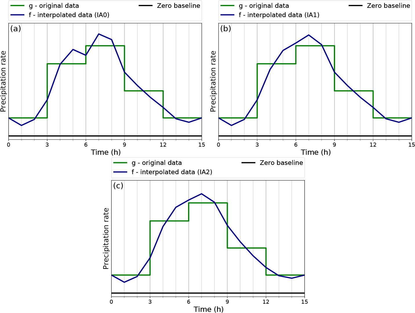
Figure 9Illustration of the basic IA0 algorithm in (a), with the additional monotonicity filter in algorithm IA1 in (b) and the directly implemented filter in the algorithm IA2 in (c). The original precipitation rate g is shown in green with a 3-hourly resolution. The IA0-interpolated data f on the new sub-grid with 1-hourly resolution are drawn in dark blue. A zero baseline is shown in black.
3.3.6 Alternative monotonicity filter yielding a single-sweep algorithm
It is also possible to construct an algorithm which directly incorporates the idea from the monotonicity filter introduced above. In order to apply the filter in a single sweep, we need a kind of educated guess for fi+2 as this appears in Eq. (31). We estimate it similar to Eq. (29) as
where the tilde indicates that it is a preliminary estimate. We can now proceed analogously to above by constructing
and determine fi+1 as
respecting again the sufficient condition for non-negativity. Having obtained fi+1, the sub-grid function values in Ii are determined as before by Eqs. (21) and (22), thus closing the algorithm. This improved version of the interpolation algorithm, with the monotonicity filter directly built in, is called Interpolation Algorithm 2 (IA2) henceforth and is also summarised in Table 1. It applies the filter to all the intervals rather than to M- or W-shaped parts of the graph only, as is the case in IA1.
Table 1Overview of the two algorithms IA1 and IA2.
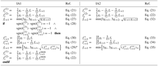
* In the original Eq. (29), the superscript “mon” to fi+1 is omitted here for simplicity.
3.4 Summary of the interpolation algorithms IA1 and IA2
Three interpolation algorithms – IA0, IA1, and IA2 – were developed. They were introduced on an additional sub-grid based on the geometric mean and fulfil the conditions to be non-negative, continuous, and area-conserving. The basic algorithm is called IA0. A monotonicity filter was then introduced to improve the realism of the reconstructed function. The IA1 algorithm requires a second sweep through the data, while IA2 has a monotonicity filter already built into the main algorithm. The equations defining IA1 and IA2 are listed in Table 1, and Fig. 9 illustrates all three with an example. The algorithms were realised in Python and can be downloaded with the Supplement.
3.5 The two-dimensional case
We have also carried out a preliminary investigation of the two-dimensional case. In the case of precipitation, this could be used for horizontal interpolation. We follow the same approach and introduce a sub-grid with two additional grid points, now for both directions.
The isolated two-dimensional precipitation event can then easily be represented on the sub-grid as a truncated pyramid. For multiple adjacent cells with non-zero data, this type of interpolation is, however, not suitable due to the non-vanishing values at the boundaries of the grids which would be difficult to formulate.
A more advantageous approach is the bilinear interpolation, which defines the function in a square uniquely through its four corner values. (Note that we assume that the grid spacing is equal in both directions, without loss of generality, as this can always be achieved by simple scaling.) The main idea here is to apply the bilinear interpolation in each of the nine sub-squares. We recall that for given function values , with , at the corners of an area , the bilinear interpolation amounts to
which corresponds to interpolating first in X at Y=Y1 and Y=Y2 and then performing another interpolation in Y (or vice versa). Thus, the algorithm is closed if the 16 sub-grid function values in each grid cell are known, where again only one is determined by the conservation of mass. The case of the isolated precipitation event with vanishing boundary values is again easily solved, since only the corner values of the centred sub-square with constant height need to be determined, amounting to 1 degree of freedom. This in particular demonstrates that the bilinear interpolation algorithm is a natural extension of the one-dimensional case, since the function value in the centred sub-square of such an isolated precipitation event turns out to be
For the general case involving larger precipitation areas many different possibilities for prescribing the slopes and function values arise at the sub-grid points. The geometric-mean-based approach can be extended to the two-dimensional setting with corresponding restrictions guaranteeing non-negativity. The derivation of a full solution for the two-dimensional case is reserved for future work.
The evaluation of the new algorithms IA1 and IA2 was carried out in three steps. First, the interpolation algorithms were applied to ideal, synthetic time series to verify the fulfilment of the requirements. Next, they were validated with ECMWF data. Short sample sections were analysed visually. The main validation is then based on statistical metrics. The original algorithm from the ECMWF data extraction for FLEXPART (flex_extract) was also included in the evaluation. In the following, it is referred to as the Interpolation algorithm FLEXPART (IFP). This allows us to see and quantify the improvements through the new algorithms. The IFP is not published, but it is included in the flex_extract download on the FLEXPART website (http://flexpart.eu/, last access: June 2018) and a Python version of it is included in the Supplement.
4.1 Verification of algorithms with synthetic data
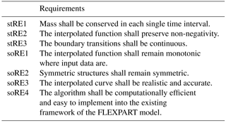
Verification is the part of evaluation where the algorithm is tested against the requirements to show whether it is doing what it is supposed to do. These requirements, mentioned in the previous sections, are classified into strict requirements (main conditions, stRE) and soft requirements (soRE), as formulated in Table 2.
Table 2Classification of requirements for the interpolation algorithm. They are classified into strict requirements (stRE), which are essential and need to be fulfilled, and soft requirements (soRE), which are desirable but not absolutely necessary.
The synthetic time series for the first tests is specified with 3-hourly resolution. It consists of four isolated precipitation events, with constant precipitation rates during the events and durations which increase from one to four 3 h intervals. As the variation within each 3 h interval is unknown, it is visualised as a step function. We refer to it as the synthesised 3-hourly (S3h) time series. Both new algorithms IA1 and IA2 and the currently used IFP were applied to these data. The IFP produces 3-hourly disaggregated output which is divided into 1 h segments by the usual linear interpolation between the supporting points. As all three algorithms are intended to be used in connection with linear interpolation, they are visualised by connecting the resulting supporting points with straight lines. Figure 10 shows the input data set together with the results from the reconstruction algorithms.
It is easy to see that IFP violates requirement stRE1 (cf. Table 2): the mass of the first precipitation event is spread over three intervals instead of one in the first event. This leads to a reduction in the precipitation intensity in the originally rainy interval while precipitation appears also in adjacent, originally dry intervals, constituting the basic problem introduced in Sect. 1. The second event is the only one in this synthetic time series where IFP conserves mass within each interval. The peak value constructed is twice the input precipitation rate. In the third event, which has a duration of three times 3 h, mass is shifted from the two outer intervals into the middle one. Similarly, in the fourth event, mass is shifted from the border to the central intervals; however, here two local maxima separated by a local minimum are created. In all these events, IFP produces a non-negative and continuous reconstruction, hence, requirements stRE2 and stRE3 are fulfilled. Concerning the soft requirements, the monotonicity condition (soRE1) may appear to be violated in the fourth event. However, some overshooting is necessary unless an instantaneous onset of the precipitation at the full rate is postulated. The symmetry condition (soRE2) is fulfilled. Requirements soRE3 and soRE4 cannot be tested well with this short and simple case.
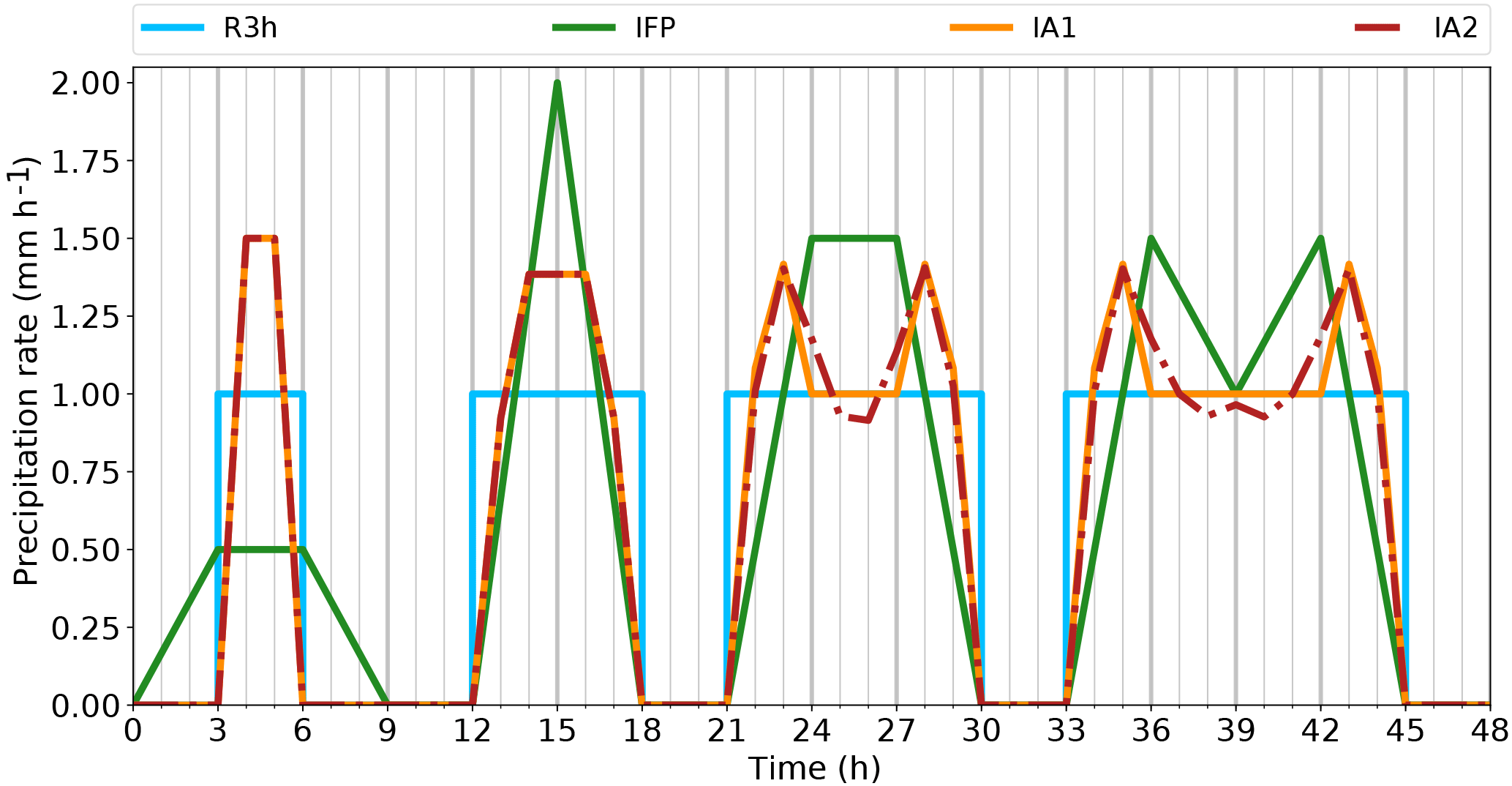
Figure 10Verification of the interpolation algorithms for four simple precipitation events. The 3-hourly synthetic precipitation rate (S3h) is illustrated as a step function in light blue. Reconstructions are shown as linear connections of their respective supporting points, with the current FLEXPART algorithm (IFP) in green, the newly developed algorithm IA1 in orange, and IA2 (also new) in red (dashed–dotted).
Concerning the behaviour of the two newly developed algorithms IA1 and IA2, we clearly see in Fig. 10 that no mass is spread from the wet intervals into the dry neighbourhood. For a strict verification of local mass conservation (stRE1), we compared the integral values in each interval of the interpolated time series and S3h numerically and found that mass is conserved perfectly for both algorithms. Moreover, non-negativity (stRE2) as well as the continuity requirement (stRE3) are also fulfilled.
With respect to soRE1 (monotonicity), we are faced with the overshooting behaviour already mentioned. In the events lasting three and four intervals, the new algorithms introduce a local minimum in the centre of the event. As directly intelligible, it is not possible for the interpolated curve to turn into a constant value without overshoot. This would either lead to excess mass in the inner period as seen in the IFP algorithm, or to a lack in the outermost periods. Obviously, interpolated curves have to overshoot to compensate for the gradual rise (or fall) near the borders of precipitation periods. While IA1 accomplishes this within a single 3 h interval, algorithm IA2 falls off more slowly towards the middle with the consequence of requiring another interval on each side for compensation. In order to investigate how these wiggles would develop in an even longer event, a case with eight constant values, lasting 24 h, was constructed (Fig. 11). It shows that the amplitude of the wiggles in IA2 falls off rapidly.
The symmetry condition (soRE2) is satisfied by IA1 but not by IA2. The wiggles in the 24 h event (Fig. 11) spread beyond the second rainy interval on the left but not on the right side. A tiny asymmetry is visible also in Fig. 10. The reason for this difference between IA1 and IA2 is the way in which the monotonicity filter is applied. In the IA1 algorithm, the filter is only applied if the curve is M- or W-shaped (Eq. 28), while in IA2 the filter is applied for each time interval. We would see in IA1 exactly the same behaviour as in IA2 if we removed the condition of Eq. (28). In the context of investigating symmetry, we have also run the reconstruction algorithms in the reverse direction. This produced identical results for IA1 but different results for IA2. We have also tried to run IA2 in both directions, taking the mean of the resulting values for the supporting points. This yields a nearly symmetrical solution (Fig. 12) and fulfils the symmetry requirement soRE2. Thus, from now on, we use this version of IA2, calling it Interpolation Algorithm 2 modified (IA2m). The question of monotonicity will be revisited with more realistic cases. As mentioned above, this idealised test case is not suitable for judging the fulfilment of soRE3 and soRE4.
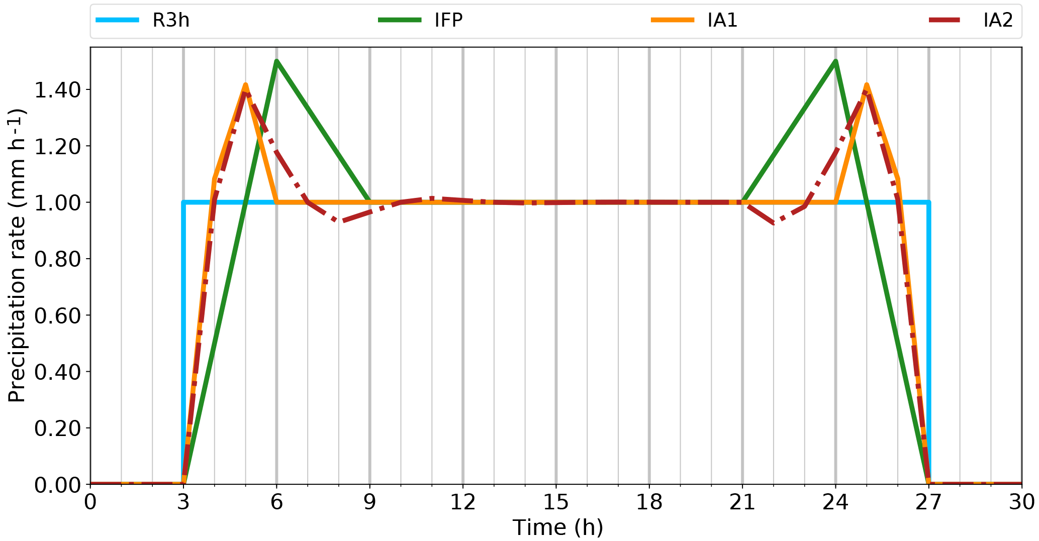
Figure 11Verification of the different behaviour of the interpolation algorithms for a longer constant precipitation event plotted in mm h−1. The 3-hourly synthesised precipitation rate (S3h) is illustrated as a step function in light blue, the old interpolation algorithm of FLEXPART (IFP) in green and the newly developed algorithms IA1 and IA2 are shown in orange and red (dashed–dotted), respectively.
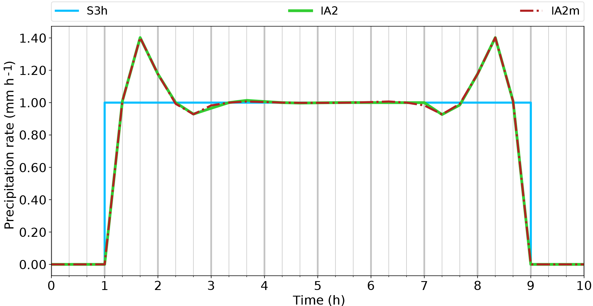
Figure 12Same as Fig. 11 but comparing only IA2 (green line) and the modified version IA2m (red; dashed–dotted). It is recommended to zoom in to see the differences clearly.
In the next step, we extended the verification to a case with more realistic but still synthetic data (Fig. 13). Again, we can see the non-conservative behaviour of the IFP algorithm. The new algorithms IA1 and IA2m conserve the mass within each single interval within machine accuracy (ca. ). As even spurious negative values need to be avoided for certain applications, values of supporting points resulting from IA1 and IA2m within the range between and zero were set to zero. All of the three strict requirements (mass conservation, non-negativity, continuity) are fulfilled.
This case provides more interesting structures for looking at monotonicity than the idealised case with constant precipitation values in each rainy period. For the new algorithms, minor violations of monotonicity can be observed, e.g. around hour 30 and a smaller one after hour 3. They occur when a strong increase of the precipitation rate is followed by a weaker one or vice versa. Thus, they represent a transition to the situation discussed above where the overshooting is unavoidable, and it is difficult to judge which overshoot is possibly still realistic. Subjectively, we would prefer an algorithm that would be less prone to this phenomenon; however, we consider this deviation from soRE1 to be tolerable. The symmetry requirement (soRE2) is not strictly tested here, as no symmetric structure was prescribed as input, but it can be noted that gross asymmetries as we see in IFP as the shifting of peaks to the border of an interval do not occur in IA1 and IA2m.
The reconstructed precipitation curves resulting from algorithms IA1 and IA2m have a more realistic shape (soRE3) than that from IFP. Due to the two additional supporting points per interval, they are able to adapt better to strong variations. Computational efficiency (soRE4) is not tested for this still short test period.
Summarising the verification with synthetic cases, it is confirmed that IA1 and IA2m fulfill all of the strict requirements whereas IFP does not. The soft requirements are fulfilled by the new algorithms with a minor deficiency for the monotonicity condition. Next, they will be validated with real data.
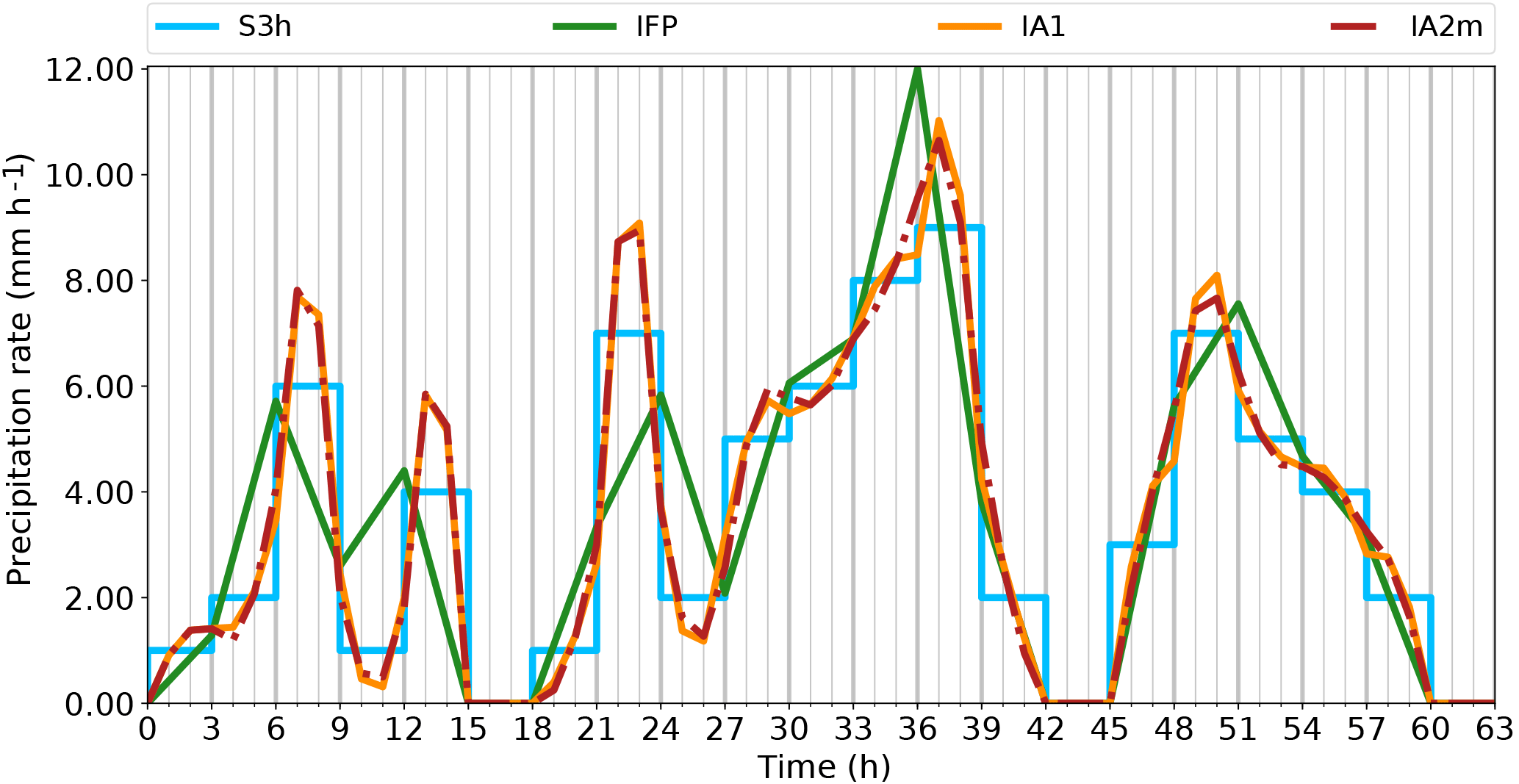
Figure 13Verification of the different behaviour of the interpolation algorithms for a complex synthetic precipitation time series. S3h is the input data series with 3 h resolution (light blue), IFP is the linearly interpolated curve according to the current scheme in FLEXPART (green), while IA1 (orange) and IA2m (red; dashed–dotted) are the reconstructions using the new algorithms.
4.2 Validation with ECWMF data
The validation with ECMWF data makes use of precipitation data retrieved with 1-hourly and 3-hourly time resolution. The 3-hourly data serve as input to the algorithms, while the 1-hourly data are used to validate the reconstructed 1-hourly precipitation amounts. In this way, the improvement of replacing IFP by one of the new algorithms can be quantified. By using a large set of data, robust results are obtained.
4.2.1 ECWMF precipitation data
Fields of both large-scale and convective precipitation in the operational deterministic forecasts were extracted from ECMWF's MARS archive with 0.5∘ resolution for the whole year 2014 and the whole globe, thus yielding approximately 2.28 × 10⁹ 1-hourly data values (720 grid points in E–W direction, 361 in N–S direction,3 8761 h including the last hour of 2013). They were extracted as 3-hourly and as 1-hourly fields. ECMWF output distinguishes these two precipitation types, derived from the grid-scale cloud microphysics scheme in the case of large-scale precipitation and from the convection scheme in the case of convective precipitation. Note that parameterised convection by definition is a sub-gridscale process, while reported precipitation intensities are averaged over the grid cell. Precipitation data are accumulated from the start of each forecast at 00:00 and 12:00 UTC. We used both these forecasts, so that the forecast lead time is at most 12 h. This is in line with typical data use in FLEXPART. Data were immediately de-accumulated to 1 and 3 h sums (see the “Data availability” section for more details).
4.2.2 Visual analysis of sample period
Two short periods in January 2014 were selected for visual inspection at a grid cell with significant precipitation, one dominated by large-scale and another one by convective precipitation. Convective precipitation occurs less frequently (cf. Table 5) and its variability is higher (cf. Table 3) than in the case of large-scale precipitation, which is more continuous and homogeneous. We are interested in the performance of the reconstruction algorithms for both of these types. Furthermore, a criterion for the selection of the sample was that it should exhibit monotonicity problems as discussed above. The two days are typical; they do not represent a rare or extreme situation. The results are shown in Fig. 14 including the reference 1- and 3-hourly ECMWF data, called R1h and R3h, respectively. Note that the same input, namely R3h, is used for all the algorithms; R1h serves for validation.
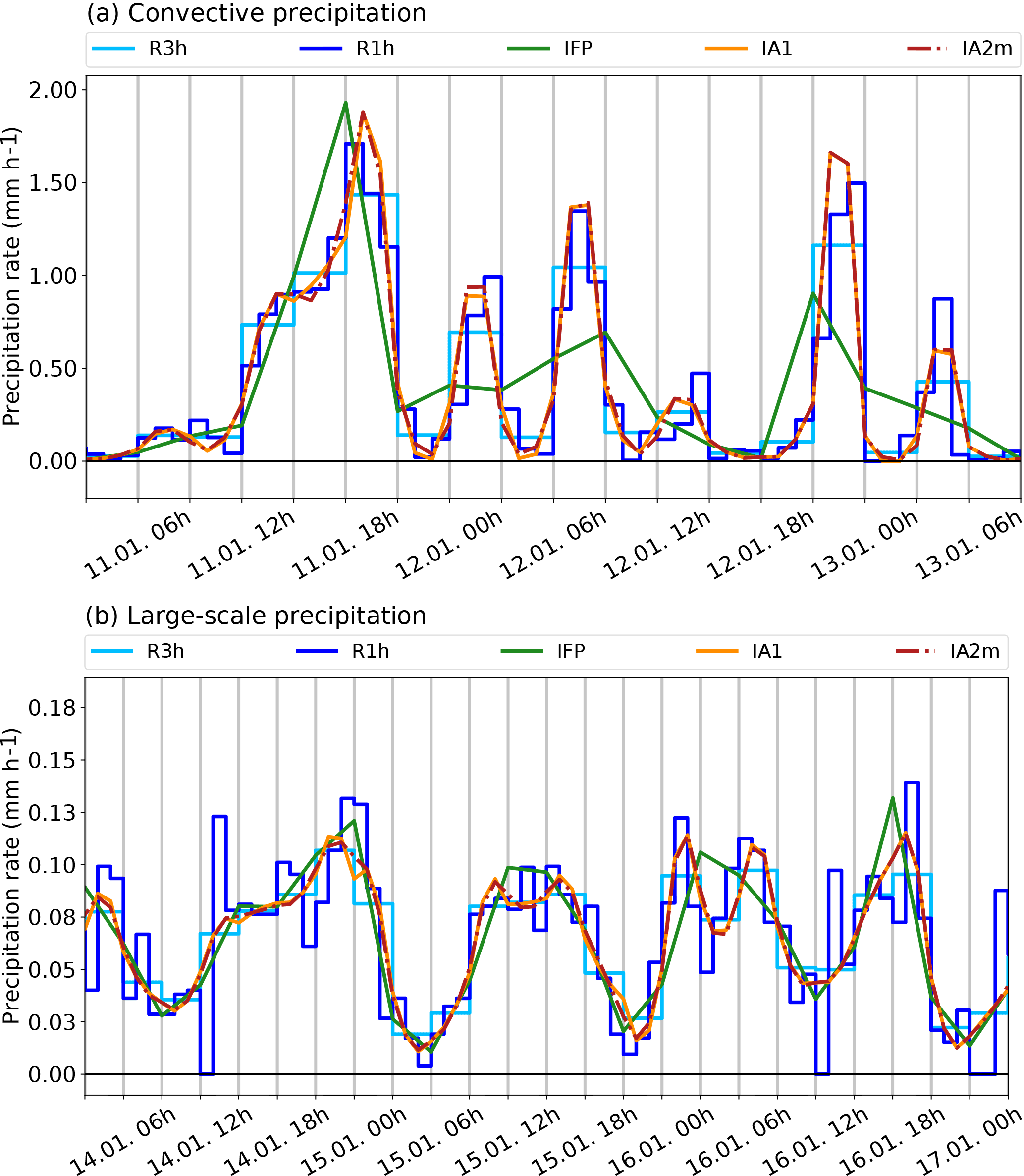
Figure 14Sample periods in January 2014 at the grid cell centred on 48∘ N, 16.5∘ W. (a) 11 January 00:00 UTC to 13 January 06:00 UTC for convective precipitation intensity, and (b) 14 January 00:00 UTC to 17 January 00:00 UTC for large-scale precipitation intensity. Original ECMWF data are shown as step functions (1-hourly: R1h – dark blue; 3-hourly: R3h – light blue), while the interpolation resulting from the reconstruction algorithms (new algorithms: IA1, orange, and IA2m, red; dashed–dotted, current FLEXPART algorithm: IFP, green) are piecewise linear between the respective supporting points. A baseline is drawn in black at intensity value zero.
Similar to the synthetic cases, large discrepancies between the real ECMWF data and the interpolated data from the IFP algorithm can be found. This is true especially for the convective precipitation, where frequently the real peaks are clipped and the mass is instead redistributed to neighbouring time intervals with lower values, leading to a significant positive bias there. The function curves of IA1 and IA2m follow the R3h signal and are even able to capture the tendency of the R1h signal as long as R1h does not have too much variability within the 3 h intervals of R3h. Again, in the convective part there is an interval where monotonicity is violated, near 11 January 12:00 UTC. The secondary minimum occurs a bit earlier in the IA1 algorithm than in the IA2m algorithm, which seems typical for the case of the ascending graph (vice versa in the descending sections; see also Fig. 13).
The large-scale precipitation rate time series is smoother and precipitation events last longer (Fig. 14). This is easier for the reconstruction with all three algorithms. Nevertheless, there are occasions which show a clear improvement compared to the old IFP algorithm, for example, the double-peak structure of the precipitation event between 15 January 18:00 UTC and 16 January 09:00 UTC, which is missing in the IFP curve but reconstructed by the new algorithms. Obviously, single-hour interruptions of precipitation cannot be exactly reconstructed and it is not possible to reproduce all the little details of the R1h time series.
Regarding the monotonicity, the large-scale precipitation time series produces a few instances with unsatisfactory monotonic behaviour, for example on 14 January 12:00 UTC or on 14 January 21:00 UTC, in the IA1 curve while the IA2m algorithm avoids the secondary minima in these cases (there are other cases where the behaviour is vice versa; not shown). The double peak structure in the IA1 and IA2m reconstructions on 15 January between 06:00 and 15:00 UTC is similar to the plateau-like ideal cases where overshooting is unavoidable.
Notwithstanding the minor problems with the monotonicity condition, the reconstructed precipitation curves from IA1 and IA2m are much closer to the real ones than the IFP curve. Therefore, we consider requirement soRE3 as basically fulfilled. This example raises the expectation that the new algorithms will be capable of improving the performance of the FLEXPART model.
Table 3Statistical metrics for the global large-scale and convective precipitation rates (mm h−1) of the ECMWF data set for the year 2014. It comprises the minimum (MIN), mean of event maxima (MEX; see text for definition), mean value (MEAN), standard deviation (SD), skewness (SKEW), and kurtosis (KURT) of the true ECMWF R3h and R1h data as well as of the data reconstructed by the current FLEXPART algorithm IFP and the two new algorithms IA1 and IA2m. Among the reconstructed data, those being closest to R1h have been marked by bold font.
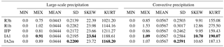
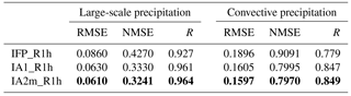
Table 4Root-mean-square error (RMSE, mm h−1), normalised root-mean-square error (NMSE), and correlation coefficient (R) between the interpolated data sets IFP, IA1, and IA2m and the true ECMWF data R1h, based on the global data set for the year 2014 and large-scale and convective precipitation. Note that NMSE is calculated only for data pairs clearly different from zero as described in the text.
4.2.3 Statistical validation
A statistical evaluation comparing the 1-hourly precipitation reconstructed by the new IA1 and IA2m algorithms as well as by the old IFP algorithm from 3-hourly input data (R3h) to the reference 1-hourly data (R1h) was carried out. While the R1h data directly represent the amount of precipitation in the respective hour, the output of the algorithms represents precipitation rates at the supporting points of the time axis, and the hourly integrals had to be calculated, under the assumption of linear interpolation. The data set comprises the whole year of 2014 and all grid cells on the globe as described in Sect. 4.2.1. All evaluations were carried out separately for large-scale and convective precipitation.
A set of basic metrics is presented in Table 3. Since all the reconstruction algorithms are conservative, either globally (IFP) or locally (IA), the overall means must be identical. This is the case for all of the 1-hourly time series. However, the average of R3h large-scale data slightly deviates from the R1h data (fourth decimal place). This can be explained as a numerical effect, as R3h averages were calculated from fewer data. All the data sets fulfil the non-negativity requirement as indicated by a minimum value of zero. The column MEX in Table 3 contains the means of the maxima of all distinct precipitation events. They were derived from R3h and are defined as consecutive intervals with a precipitation rate of at least 0.2 mm h−1 in each interval bounded by at least one interval with less than 0.2 mm h−1. The periods thus derived are also used for the 1-hourly time series. The mean of all event maxima in R1h is best reproduced by the IA1 algorithm which underestimates it by about 10 % for large-scale and 30 % for convective precipitation, whereas the underestimation is considerably larger in IFP, about 20 % and, respectively, 45 %. The higher-order moments (standard deviation, skewness, kurtosis) serve to measure the similarity of the distributions; for precipitation, the skewness is of specific interest as it characterises the relative frequency of high values. They are generally underestimated by the reconstruction algorithms. However, the new algorithms are always closer to the R1h values than the IFP values. An exception is the kurtosis of the large-scale precipitation which is overestimated (again, less by IA1 and IA2m than by IFP).
The root mean square error (RMSE), the normalised root mean square error (NMSE), and the correlation coefficient (R) between the R1h and the reconstructed data are listed in Table 4. The NMSE is calculated as
where only cases with are considered, N being the total number of these cases. The new methods represent a clear improvement compared to the IFP method, with IA2m being slightly better than IA1 with respect to all parameters. The large-scale precipitation reconstruction is obviously more accurate than that of the convective precipitation, even though this gap is reduced by IA1 and IA2m.
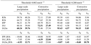
Another aspect is the ability of the algorithms to conserve the ratio of dry and wet intervals (Table 5). Two different thresholds of the precipitation intensity were chosen to separate “dry” and “wet”. The lower one, 0.002 mm h−1 corresponds to about 0.05 mm day−1 (rounded to 0.1 mm, the lowest non-zero value reported by meteorological stations). The higher one is 0.2 mm h−1 and indicates substantial rain or snowfall. Again, the results are reported separately for large-scale and convective precipitation. In all cases, the reconstructions produce too many wet intervals. The relative deviations are larger for the lower threshold and for convective precipitation in comparison to large-scale precipitation. In all cases, the new algorithms result in a clear improvement compared to the current IFP algorithm. For the high threshold and large-scale precipitation; however, already IFP deviates only by 1.9 %; for convective precipitation, the relative deviation is improved from 15 to 11 %. In the case of the lower threshold, the improvement is from 18 to 13 % and 35 to 23 %, the latter for convective precipitation. The differences between IA1 and IA2m are marginal, with the latter being better in three of the four situations.
Table 5Frequencies of dry (hd) and wet (hw) intervals in the reference (R3h, R1h) and interpolated (IFP, IA1, IA2m) precipitation data (upper part), based on the global data set for the year 2014. Relative deviations (δd and δw) between the three interpolations and R1h are shown in the lower part. Two different thresholds (0.2 and 0.002 mm h−1) were used to separate “wet” and “dry”. Large-scale and convective precipitation were analysed separately. All values are in percent. The reconstructed values that match best the true R1h data are printed in bold.
Finally, two-dimensional histograms (relative frequency distributions) are provided for a more detailed insight into the relationship between the reconstructed and the true R1h values (Fig. 15). The larger scatter in the convective precipitation compared to the large-scale one is striking.
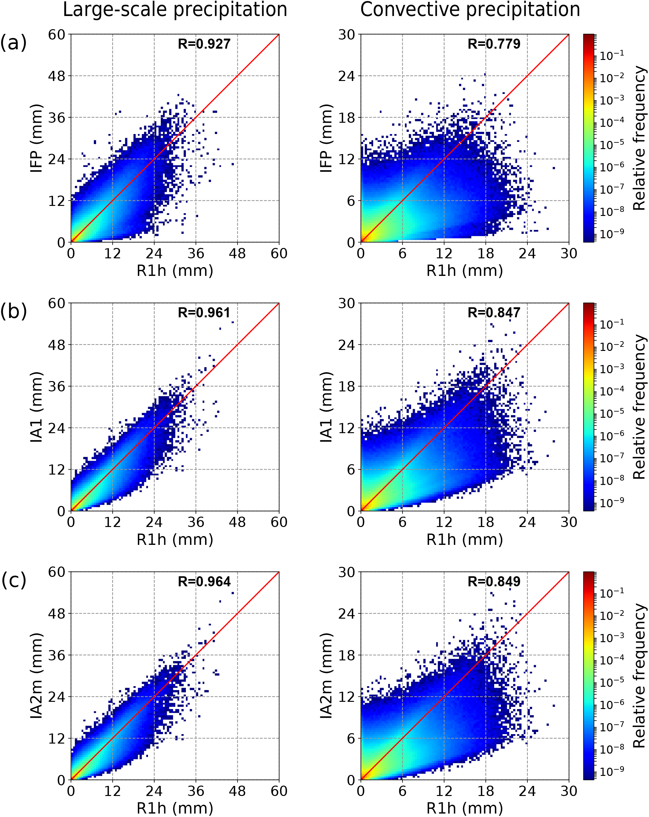
Figure 15Two-dimensional histogram (relative frequencies) showing the relationship between the hourly precipitation reconstructed by (a) IFP, (b) IA1, and (c) IA2m and the true R1h precipitation, based on the global data set for the year 2014. For each axis, 100 equally distributed bins were used. The correlation coefficient is given in each plot, and the one-to-one line is shown in red.
The distributions are clearly asymmetric with respect to the diagonal, especially for the convective precipitation. One has to be careful in the interpretation, however, because most cases are concentrated in the lower left corner (log scale for the frequencies, spanning many orders of magnitude). Thus, at least for the high values, more points fall below the diagonal, indicating more frequent underprediction. This might be due to the short duration of peaks with the highest intensity. For both precipitation types, but especially for convective precipitation, an overestimation of very low intensities is noticeable. Zooming in, the first R1h bin for the convective precipitation shows enhanced values corresponding to the bias towards wet cases in Table 5. This is continued as a general levelling off of (imagined) frequency isolines towards the y axis, which corresponds to the weaker but still present wet bias with higher thresholds. Another feature for the convective precipitation is the structure noticeable in the sector below the diagonal. Especially in the IFP plot, a secondary maximum is visible in the light-blue area, indicating a characteristic severe underprediction. This is less pronounced for IA1 and almost absent for IA2m. Summarising, the scatter plots indicate an improvement from IFP towards IA1 and IA2m. A near-perfect agreement obviously cannot be expected as the information content in the 3 h input data is of course less than in the 1 h data. This information gap is larger for the convective precipitation which obviously has a shorter autocorrelation timescale.
4.3 Performance
Potential applications for the new algorithm include situations where computational performance is relevant. For the precipitation (and possibly other input data; see Sect. 5), both the time for the preprocessing software flex_extract (which includes the reconstruction algorithm to calculate the supporting points) and time for interpolation in FLEXPART itself are relevant, and they should not significantly exceed the current computational efforts.
During the evaluation process, a computationally more efficient version of the IA1 algorithm was developed. It applies the monotonicity filter within one sweep through the time series (filter trailing behind the reconstruction) rather than processing the series twice. The algorithmic equations are unchanged. We refer to this version as speed-optimised Interpolation Algorithm 1 (IA1s). It was verified that results are not different from the standard IA1.
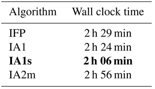
The wall clock time for the application of each of the algorithms to the 1-year global test data set is listed in Table 6. This is the time needed to reconstruct the new time series with Python and to save the data in the npz format provided by Python's NumPy package, which is the most efficient way to write them out. The computing time for all the new algorithms is similar to that of the old algorithm. The fastest version is IA1s, which needs about 85 % of the time required by IFP, while the IA2m, the slowest version, takes about 118 % of IFP.
Table 6Computing time (wall clock) for the processing of 1-year of global data (ECMWF test data used in this paper) with the old IFP algorithm and the new IA1, IA1s, and IA2m algorithms, on a Linux server with Intel(R) Xeon(R) E5-2690 @ 2.90 GHz CPU, single thread. The fastest algorithm is marked in bold.
5.1 Conclusions
We have provided a one-dimensional, conservative, and positively definite reconstruction algorithm suitable for the interpolation of a gridded function whose grid values represent integrals over the grid cell, such as precipitation output from numerical models. The approach is based on a one-dimensional piecewise linear function with two additional supporting points within each grid cell, dividing the interval into three pieces.
This approach has three degrees of freedom, similar to a piecewise parabolic polynomial. They are fixed through the mass conservation condition, the slope of the central interval which is taken as the average of the slopes of the two outer subintervals, and the left and right border grid points (each counting as half a degree of freedom). For the latter, the geometric mean value of the bordering integral values is chosen. Its main advantage is that the function values vanish automatically if one of the involved values is zero, which is a necessary condition for continuity. However, the geometric mean in general converges too slowly with vanishing values to prevent negative values under all conditions. This led us further to derive a sufficient condition for non-negativity and restrict the function values accordingly by these upper bounds.
This non-negative geometric-mean-based algorithm, however, still violates monotonicity. Therefore, we further introduced a (conservative) filter for regions where the remapping function takes an M- or W-like shape, requiring a second run through the data (IA1). Alternatively, the filter can be applied during the first sweep immediately after the construction of the next interval (IA1s). We also showed how this basic idea of the monotonicity filter can be directly incorporated into the construction of an algorithm (IA2). As in this case the algorithm is not symmetric, we apply it a second time in the other direction and average the results (IA2m).
The evaluation, consisting of verification and validation, confirmed the advantages of the new algorithms IA1 (including IA1s) and IA2m. After the verification of our requirements, each evaluation step revealed a significant improvement by the new algorithms as compared to the algorithm currently used for the FLEXPART model. Nevertheless, the soft requirement of monotonicity has not been fulfilled perfectly, but the deviation is considered to be acceptable. The modified version of IA1 (IA1s) yields identical results to IA1 and is quite fast. However, the results of the quantitative statistical validation would slightly favour the IA2m algorithm, whose computational performance is still acceptable, even though in this modified form the original IA2 algorithm is applied twice.
5.2 Outlook
The next steps will be the integration of the method into the preprocessing of the meteorological input data for the FLEXPART Lagrangian dispersion model and the model itself for the temporal interpolation of precipitation. The application to two dimensions, intended for spatial interpolation, is also under investigation. Options include the straightforward operator-splitting approach as well as an extension based on bilinear interpolation with additional supporting points. As the monotonicity filter appears to be not yet perfect, this may also be revisited.
5.3 Possible other applications of the new piecewise linear reconstruction method
It may be noted that there is a wide range of useful applications of such conservative reconstructions. Interestingly, at least in the geoscientific modelling community, they have largely remained restricted to the specific problem of semi-Lagrangian advection schemes. Therefore, we sketch out more possible use cases below.
In typical LPDMs, other extensive quantities which are being used, apart from precipitation, are surface fluxes of heat and momentum which enter boundary-layer parameter calculations and which could be treated similarly, especially for temporal interpolation. The often-used 3-hourly input interval is quite coarse and may, for example, clip the peak values of the turbulent heat flux.
In many applications, output is required for single points representing measurement stations or, in the case of backward runs (Seibert and Frank, 2004), point emitters. While FLEXPART has the option of calculating concentrations at point receptors with a parabolic sampling kernel, the results have often been similar to simple bilinear interpolation of gridded output, probably because of the difficulty of determining an optimum kernel width; therefore, many users produce only the gridded output and take the point values through a nearest-neighbour or a bilinear interpolation approach. The piecewise linear interpolation with additional supporting points as introduced here or one of the higher-order methods discussed in Sect. 2 would probably provide an improvement.
This latter example could be easily extended to all kinds of model output postprocessing, where currently methods that are too simple often prevail. It should be clear that applying naive bilinear interpolation to gridded output of precipitation and other extensive quantities, including fluxes, introduces systematic errors as highlighted in Sect. 1.
Finally, this also includes contouring software. Contouring involves interpolation between neighbouring supporting points to determine where the contour line should intersect the cell boundaries. It is obvious that linear interpolation is inadequate for extensive quantities whose values represent grid averages. This holds in particular for precipitation, energy fluxes, and trace species concentrations. While we cannot expect the many contouring packages to be rewritten with an option for conservative interpolation, our method (once extended to two dimensions) provides an easy implementation through preprocessing resulting in an auxiliary grid with triple (one-dimensional) resolution that then could be linearly interpolated without violating mass conservation, thus enabling it to be used with standard contouring software.
The piecewise linear reconstruction routines IA1, IA2, and IA1s are written in Python2. The code is included in the Supplement and is licensed under the Creative Commons Attribution 4.0 International License. For IA2m, IA2 has to be called with the original and the reversed time series and the results have to be averaged. The software for the statistical evaluation (written in Python2) is available on request by contacting the second author, A. Philipp (anne.philipp@univie.ac.at). It relies on the NumPy (van der Walt et al., 2011) and SciPy (Jones et al., 2001) libraries for data handling and statistics and on Matplotlib (Hunter, 2007) for the visualisation. The FLEXPART model as well as the accompanying data extraction software can be downloaded from the community site: http://flexpart.eu/ (last access: June 2018).
The precipitation data used for evaluating the interpolation algorithms were extracted from ECMWF through MARS retrievals (ECMWF, 2017). For easy reproducibility of the results, we provide the MARS retrieval routines in the Supplement, licensed under the Creative Commons Attribution 4.0 International License. Note that only authorised ECMWF users have access to the operational archive data.
We show in the following that the monotonicity filter as introduced in Sect. 3.3.5 improves the monotonicity behaviour and also does not destroy non-negativity. The conservation of mass (equal-area condition) is clearly preserved by construction.
- i.
The M-shape: this corresponds to the case
Then, the filter improves the monotonicity behaviour in the sense that
To see this we note that according to Eq. (17), the conditions and are equivalent to
Furthermore, from the condition , we can deduce
implying in particular also
From the condition , we can deduce in a similar fashion that
such that in particular also
Making use of all derived inequalities, we can deduce
- ii.
The W-shape: this corresponds to the case
Again the filter improves the monotonicity behaviour in the sense that
Arguing similarly, now the conditions and imply
and thus in particular
This can be easily proven by contradiction, since otherwise if (or ), then also fi≤3gi (or , respectively) by construction, implying furthermore (or ), which obviously contradicts (Eq. A8). From the condition , we can deduce in a similar way as above
From , we accordingly obtain
Note that in comparison to the M-shape above, there is no lower bound for the different constructed values , . Thus, they can take possibly negative values and care has to be taken here to ensure that the filter still preserves non-negativity. Combining Eqs. (A9), (A10), and (A11), we can now deduce
The supplement related to this article is available online at: https://doi.org/10.5194/gmd-11-2503-2018-supplement.
PS formulated the problem in Sect. 1, made initial suggestions, and guided the work. Section 2 was jointly written by SH and PS. Section 3 and Appendix A were contributed mainly by SH (with additions by AP); Sect. 4 is by AP. Section 5 was written jointly by all authors. The Supplement was contributed by AP.
The authors declare that they have no conflict of interest.
Sabine Hittmeir thanks the Austrian Science Fund (FWF) for the support via
the Hertha Firnberg project T-764-N32, which also finances the open-access
publication. We thank the Austrian Meteorological Service ZAMG for access to
the ECMWF data. The second and third author are grateful to Christoph Erath
(then Department of Mathematics, University of Vienna; now at TU Darmstadt,
Germany) for an early stage discussion of the problem and useful suggestions
about literature from the semi-Lagrangian advection community. We also thank
the reviewers for careful reading, thus helping to improve the
paper.
Edited by: Simon Unterstrasser
Reviewed by: Wayne Angevine and one anonymous referee
ECMWF: MARS User Documentation, available at: https://software.ecmwf.int/wiki/display/UDOC/MARS+user+documentation, last access: 10 August 2017. a
Hämmerlin, G. and Hoffmann, K.-H.: Numerische Mathematik, Springer, 4th Edn., https://doi.org/10.1007/978-3-642-57894-6, 1994. a
Hermann, M.: Numerische Mathematik, München Oldenburg, 3rd Edn., 2011. a
Hunter, J. D.: Matplotlib: A 2D graphics environment, Comput. Sci. Eng., 9, 90–95, https://doi.org/10.1109/MCSE.2007.55, 2007. a
Jones, E., Oliphant, T., Peterson, P., et al.: SciPy: Open source scientific tools for Python, available at: http://www.scipy.org/ (last access: 10 August 2017), 2001–2017. a
Lauritzen, P. H., Ullrich, P. A., and Nair, R. D.: Atmospheric transport schemes: Desirable properties and a semi-Lagrangian view on finite-volume discretizations, in: Numerical Techniques for Global Atmospheric Models, edited by: Lauritzen, P. H., Jablonski, C., Taylor, M. A., and Nair, R. D., Lect. Notes Comp. Sci., 80, 185–250, https://doi.org/10.1007/978-3-642-11640-7_8, 2010. a
Lin, J. C., Brunner, D., Gerbig, C., Stohl, A., Luhar, A., and Webley, P. (Eds.): Lagrangian Modeling of the Atmosphere, in: Geophysical Monograph Series, 26, https://doi.org/10.1029/GM200, 2013. a
Schmidt, J. W. and Heß, W.: Positivity of cubic polynomials on intervals and positive spline interpolation, BIT, 28, 340–352, https://doi.org/10.1007/BF01934097, 1988. a
Seibert, P. and Frank, A.: Source-receptor matrix calculation with a Lagrangian particle dispersion model in backward mode, Atmos. Chem. Phys., 4, 51–63, https://doi.org/10.5194/acp-4-51-2004, 2004. a
Stohl, A., Forster, C., Frank, A., Seibert, P., and Wotawa, G.: Technical note: The Lagrangian particle dispersion model FLEXPART version 6.2, Atmos. Chem. Phys., 5, 2461–2474, https://doi.org/10.5194/acp-5-2461-2005, 2005. a, b
van der Walt, S., Colbert, S. C., and Varoquaux, G.: The NumPy array: A structure for efficient numerical computation, Comput. Sci. Eng., 13, 22–30, https://doi.org/10.1109/MCSE.2011.37, 2011. a
White, L., Adcroft, A., and Hallbert, R.: High-order regridding-remapping schemes for continuous isopycnal and generalized coordinates in ocean models, J. Comput. Phys., 228, 8665–8692, https://doi.org/10.1016/j.jcp.2009.08.016, 2009. a
Zerroukat, M., Wood, N., and Staniforth, A.: SLICE: A Semi-Lagrangian Inherently Conserving and Efficient scheme for transport problems, Q. J. Roy. Meteor. Soc., 128, 2801–2820, https://doi.org/10.1256/qj.02.69, 2002. a
Zerroukat, M., Wood, N., and Staniforth, A.: A monotone and positive-definite filter for a Semi-Lagrangian Inherently Conserving and Efficient (SLICE) scheme, Q. J. Roy. Meteor. Soc., 131, 2923–2936, https://doi.org/10.1256/qj.04.97, 2005. a, b
Zerroukat, M., Wood, N., and Staniforth, A.: The Parabolic Spline Method (PSM) for conservative transport problems, Int. J. Numer. Meth. Fl., 51, 1297–1318, https://doi.org/10.1002/fld.1154, 2006. a
This software is available from the FLEXPART community website in different versions as described in https://www.flexpart.eu/wiki/FpInputMetEcmwf (last access: June 2018).
In reality, the problem is even more complex. In ECMWF's MARS archive, variables such as precipitation are stored on a reduced Gaussian grid, and upon extraction to the latitude–longitude grid they are interpolated without paying attention to mass conservation. This needs to be addressed in the future on the level of the software used internally by MARS. Our discussion here is assuming that this would already have happened, and even if that is not the case, adding another step of non-mass-conserving interpolation makes things even worse.
As explained in footnote 2, currently the precipitation extracted on a lat–long grid is a point value. As the global grid includes the poles, there are 361 points per meridian. Nevertheless, as explained, we also use the concept of a cell horizontally, as does FLEXPART.
- Abstract
- Motivation
- Possible approaches and related literature
- Derivation of the interpolation algorithm
- Evaluation of interpolation algorithms
- Conclusions and outlook
- Code availability
- Data availability
- Appendix A: Theoretical aspects of the monotonicity filter
- Author contributions
- Competing interests
- Acknowledgements
- References
- Supplement