Development and evaluation of the ECHAM6-iMAPLE v1.0 coupled atmosphere–ecosystem model

Land–atmosphere interactions play a fundamental role in regulating climate variability, ecosystem productivity, and air quality through coupled exchanges of energy, water, carbon, and reactive trace gases. However, many Earth system models adopt simplified representations of vegetation physiological processes, leading to biases in terrestrial carbon and water fluxes and increased uncertainties in climate simulations. Here, we present ECHAM6-iMAPLE v1.0, a newly coupled modeling framework that integrates the interactive Model for Air Pollution and Land Ecosystems (iMAPLE v1.0) into the ECHAM6 atmospheric general circulation model, replacing carbon and water fluxes simulated by the original JSBACH vegetation module. The coupled model is evaluated against reanalysis, benchmark, and satellite datasets. Compared with the original ECHAM6–JSBACH configuration, ECHAM6-iMAPLE substantially improves simulations of gross primary productivity, evapotranspiration, and leaf area index, capturing their spatial distributions and seasonal cycles more reasonably. These improvements arise from well-constrained physiological parameters calibrated using extensive site-level observations and a more realistic representation of key biophysical processes in iMAPLE. With improved carbon and water fluxes, simulations of soil temperature, soil moisture, and surface air temperature show reduced root mean square errors. Overall, evaluations demonstrate that ECHAM6-iMAPLE provides a useful tool for investigating atmosphere–ecosystem interactions and their implications for future climate change projections.

1 Introduction

Terrestrial ecosystems and climate systems are tightly linked through exchanges of energy fluxes, water vapor, carbon, and trace gases, thereby regulating regional and global climate patterns (Pielke et al., 1998; Green et al., 2017). Climate conditions directly influence vegetation growth (Parmesan and Yohe, 2003; Fastovich et al., 2025), distribution (Seidl et al., 2017; Nolan et al., 2018), and phenology (Higgins et al., 2023), and atmospheric pollutants such as ozone can damage plant physiological processes by reducing photosynthetic rates and stomatal conductance (Sitch et al., 2007; Cao et al., 2024). Conversely, terrestrial ecosystems exert substantial feedbacks on the atmosphere through physical and biogeochemical processes (Bonan, 2008; Heimann and Reichstein, 2008). For instance, terrestrial vegetation absorbs approximately 120 Pg C yr⁻¹ through photosynthesis (Beer et al., 2010; Friedlingstein et al., 2025), while vegetation and soil respiration return a comparable amount of CO₂ into the atmosphere (Ruehr et al., 2023). Ecosystems also influences the partitioning of sensible and latent heat fluxes by modulating transpiration and canopy conductance (Williams and Torn, 2015; Zeng et al., 2017; Forzieri et al., 2020), thus affecting precipitation patterns and the intensity/frequency of hydrological extremes (Zhou et al., 2021; Schumacher et al., 2022; Zhang et al., 2025).

Models that couple atmospheric general circulation with vegetation dynamics provide essential tools for investigating interactions between the atmosphere and terrestrial ecosystems (Sellers et al., 1997; Berg et al., 2016). However, vegetation models differ substantially in their parameterization schemes for representing complex hydrological, biogeophysical, and biogeochemical processes. Uncertainties arising from these parameterization differences can propagate through land–atmosphere interactions, thereby influencing weather forecasts and climate projections (Wei et al., 2010, 2018). Despite continuous development, many widely used vegetation models still lack a comprehensive representation of key ecosystem processes that regulate land-atmosphere exchanges of energy, water, and biogeochemical constituents (Pitman, 2003; Blyth et al., 2021). For instance, vegetation dynamics such as seasonal variations of leaf area are usually prescribed with empirical parameters rather than being simulated through interactive responses to environmental drivers (Gulden et al., 2007; Niu et al., 2011; Fisher and Koven, 2020). This limitation constrains the ability of models to realistically capture ecosystem dynamics and their feedbacks to the atmosphere.

In this study, we present the coupled atmosphere–ecosystem model ECHAM6-iMAPLE, developed by integrating the interactive Model for Air Pollution and Land Ecosystems (iMAPLE) v1.0 (Yue et al., 2024) into the atmospheric general circulation model ECHAM version 6.3 (https://redmine.hammoz.ethz.ch/projects/hammoz, last access: 30 March 2026) (Tegen et al., 2019). ECHAM6 has been extensively developed with multiple Earth system components and has participated in the Sixth Coupled Model Intercomparison Project (CMIP6) (Stevens et al., 2013; Sidorenko et al., 2015; Cao et al., 2018). The original ECHAM6 model employs the Jena Scheme for Biosphere–Atmosphere Coupling in Hamburg (JSBACH) to represent vegetation dynamics and terrestrial carbon cycling (Giorgetta et al., 2013). Here, we replace the carbon and water simulations by JSBACH with iMAPLE, a global dynamic vegetation model designed to simulate plant growth and terrestrial carbon cycle interactively (Yue et al., 2024). Both JSBACH and iMAPLE have been evaluated offline in the multi-model intercomparison project for Global Carbon Budget, where iMAPLE shows improved performance in simulating key carbon and water fluxes compared with JSBACH (Friedlingstein et al., 2025). We evaluate the dynamically simulated carbon and water fluxes from ECHAM6-iMAPLE, and compare them with simulations using the original ECHAM6-JSBACH framework. In particular, we investigate whether the updated vegetation representation improves the simulation of critical land-surface variables, including soil temperature, soil moisture, near-surface air temperature, and precipitation. A detailed description of the model coupling framework is provided in Sect. 2. Section 3 presents the simulation results and model evaluations. Concluding remarks and future research perspectives are discussed in Sect. 4.

2 Models, methods, and data

2.1 Descriptions of iMAPLE

iMAPLE is an interactive model developed to investigate the interplay between air pollution and terrestrial ecosystems (Yue et al., 2024). The model evolved from version 1.0 of the Yale Interactive terrestrial Biosphere (YIBs) model, with an expanded focus on explicitly representing the interaction between atmospheric chemistry and land ecosystems (Yue and Unger, 2015). Compared to YIBs, iMAPLE incorporates several new processes, including dynamic fire emission (Pechony and Shindell, 2009; Li et al., 2012), wetland methane emissions (Walter et al., 2001; Zhu et al., 2014), and photosynthetic limitation under environmental stress (Arora et al., 2009). Furthermore, iMAPLE integrates the process-based hydrological scheme Noah-MP, including precipitation partitioning, infiltration, soil moisture redistribution, evapotranspiration, runoff generation, and groundwater-related processes. This enables dynamical simulation of soil temperature and moisture and facilitates tight coupling between the carbon (simulated by YIBs) and water (simulated by Noah-MP) cycles (Niu et al., 2011). These improvements substantially enhance the model's capacity to represent ecosystem–atmosphere interactions. Below, we briefly describe the parameterizations of vegetation biophysics and hydrological processes. A comprehensive model description is provided in Yue et al. (2024) and Niu et al. (2011).

2.1.1 Vegetation biophysics of iMAPLE

The vegetation biophysics in iMAPLE utilizes the canonical Michaelis–Menten enzyme-kinetics scheme to simulate photosynthetic processes for both C₃ and C₄ plant functional types (Farquhar et al., 1980; Von Caemmerer and Farquhar, 1981). The total leaf photosynthesis (A_tot, µmol m⁻² s⁻¹) is limited by one of three biochemical processes:

$$\begin{array}{}\text{(1)}& A_{\mathrm{tot}}=\min \left(J_{\mathrm{c}},J_{\mathrm{e}},J_{\mathrm{s}}\right).\end{array}$$

Here, J_c represents the Rubisco-limited rate of carbon fixation catalyzed by the enzyme ribulose 1,5-bisphosphate (RuBP) carboxylase/oxygenase (Rubisco). J_e  enotes the RuBP regeneration-limited rate driven by electron transport through the Calvin cycle and associated thylakoid reactions. J_s is the limitation imposed by end-product synthesis, reflecting the capacity for starch and sucrose formation to regenerate inorganic phosphate required for photophosphorylation in C₃ plants, or phosphoenolpyruvate (PEP) regeneration in C₄ plants. The rates J_c, J_e, and J_s are parameterized as functions of environmental meteorological conditions and photosynthetic capacity, including the maximum carboxylation rate (V_cmax, µmol m⁻² s⁻¹) (Collatz et al., 1991, 1992). V_cmax is derived from its optimum value at 25 °C (V_cmax25) through a temperature-dependent Q₁₀  unction. PFT-specific V_cmax25 values have been calibrated against extensive site-level eddy covariance measurements from more than 200 FLUXNET sites (Yue et al., 2024).

The canopy radiative transfer scheme employs an adaptive approach, typically dividing vegetation into 2–16 vertical layers to resolve light stratification within the canopy. At each layer, a two-leaf approach further partitions leaf area into sunlit and shaded fractions, thereby capturing canopy light heterogeneity and distinguishing the different light-use efficiency under diffuse and direct radiation (Spitters, 1986; Spitters et al., 1986). Gross primary productivity (GPP) is then calculated by integrating photosynthesis across all leaf area index (LAI):

$$\begin{array}{}\text{(2)}& \mathrm{GPP}=\int {\mathrm{0}}^{\mathrm{LAI}}{A}_{\mathrm{tot}}dL.\end{array}$$

Phenology in iMAPLE is represented by a prognostic phenological factor (f) that is updated daily. The phenology scheme is based on the framework of Kim et al. (2015) and was refined using multi-year LAI measurements at four US forest sites and leaf phenology records from hundreds of ground sites within the US National Phenology Network (Yue et al., 2015). For short-stature vegetation such as tundra, savanna, and shrubland, the phenological state is governed by temperature and/or soil moisture, with the dominant control set by PFT and regional climate (Delbart and Picard, 2007). Deciduous forests likewise use temperature- and moisture-dependent thresholds, whereas evergreen needleleaf and evergreen broadleaf PFTs adopt a constant phenological factor, with frost hardening applied to reduce V_cmax for needleleaf forests in cold seasons. Cropland phenology is prescribed from planting and harvest calendars. LAI is updated at 10-day intervals based on total leaf carbon and vegetation phenology:

$$\begin{array}{}\text{(3)}& \mathrm{LAI}=f\times {\mathrm{LAI}}_{\mathrm{b}}.\end{array}$$

Here, LAI_b is related to vegetation carbon, which is the sum of carbons in leaf (C₁), root (C_r), and stem pools (C_w):

$$\begin{array}{}\text{(4)}& C_{\mathrm{veg}}=C_{\mathrm{1}}+C_{\mathrm{r}}+C_{\mathrm{w}}.\end{array}$$

As a result, carbon assimilation determines the total carbon available for allocation, whereas carbon allocation dynamically regulates vegetation development (Cox, 2001; Clark et al., 2011).

2.1.2 Water cycle of iMAPLE

The hydrological cycle in iMAPLE adopts the Noah-MP module, which resolves the grid-scale water balance among precipitation (P, kg m⁻² s⁻¹), evapotranspiration (ET, kg m⁻² s⁻¹), runoff, and changes in terrestrial water storage (ΔTWS) at each grid:

$$\begin{array}{}\text{(5)}& P=\mathrm{ET}+\mathrm{runoff}+\mathrm{\Delta }\mathrm{TWS}.\end{array}$$

ET is further divided into plant transpiration (E_tr), canopy evaporation (E_can), and ground evaporation (E_gro):

$$\begin{array}{}\text{(6)}& \mathrm{ET}=E_{\mathrm{tr}}+E_{\mathrm{can}}+E_{\mathrm{gro}}.\end{array}$$

The runoff comprises surface (R_srf) and subsurface (R_sub) parts:

$$\begin{array}{}\text{(7)}& \mathrm{runoff}=R_{\mathrm{srf}}+R_{\mathrm{sub}}.\end{array}$$

Terrestrial water storage (TWS) encompasses three major components: groundwater storage (W_gw), which refers to water held in aquifers; soil water content (W_soil), representing moisture within four soil layers (N_soil=4); and snow water equivalent (W_snow), indicating the liquid water equivalent of accumulated snowpack:

$$\begin{array}{}\text{(8)}& \mathrm{TWS}=W_{\mathrm{gw}}+W_{\mathrm{snow}}+\sum _{i=\mathrm{1}}^{N_{\mathrm{soil}}=\mathrm{4}}{W}_{\mathrm{soil}}.\end{array}$$

Groundwater is treated explicitly in Noah-MP through the simple groundwater model (SIMGM) (Niu et al., 2007). An unconfined aquifer is placed beneath the soil column; aquifer water storage (W_a) evolves through recharge and discharge, and the water-table depth is diagnosed from W_a.

2.2 Descriptions of ECHAM v6.3

ECHAM6 is the sixth generation of the ECHAM atmospheric general circulation model, developed by the Max Planck Institute for Meteorology (MPI-M) (Giorgetta et al., 2013; Stevens et al., 2013). Its dynamical core employs a hybrid numerical framework that combines spectral and finite-difference methods to solve the primitive equations (Arakawa, 1966; Bourke et al., 1977). Horizontally, ECHAM6 utilizes a truncated spherical harmonic expansion to calculate the nonlinear and parameterized terms of dynamical fields on a Gaussian grid. Vertically, the model employs a hybrid sigma-pressure coordinate system implemented on a Lorenz grid (Phillips, 1957; Simmons and Burridge, 1981). Turbulent mixing in the atmosphere is represented by a turbulent kinetic energy (TKE) scheme, and surface fluxes are computed using bulk transfer coefficients with Louis-type stability functions based on the bulk Richardson number (Louis, 1979; Brinkop and Roeckner, 1995). Land roughness lengths are provided by JSBACH and evolve with the surface state.

Compared to previous ECHAM versions, ECHAM6 incorporates substantial improvements in key physical processes, including a more sophisticated representation of land surface processes, updated radiation parameterizations, refined surface albedo calculations, and revised convection triggering criteria (Stier et al., 2005; Crueger et al., 2018; Tegen et al., 2019). In the default ECHAM6 configuration, land-surface processes are handled by JSBACH. After coupling with iMAPLE, JSBACH remains responsible for most land-surface calculations in ECHAM6, whereas iMAPLE is used for vegetation processes. Details of the exchanged variables are given in Sect. 2.3. The model supports multiple configurations, with horizontal resolutions spanning from T31 (3.75°) to T255 (0.7°) and 47 or 95 vertical layers (Stevens et al., 2013). In this study, we adopt the T63L47 configuration to enable coupling with the iMAPLE model. The T63 spectral grid is characterized by an approximate grid spacing of 1.875° in longitude and latitude. The L47 vertical configuration comprises 47 layers extending from the surface to 0.01 hPa.

ECHAM6 employs JSBACH version 3.10 to simulate land vegetation processes (Goll et al., 2017). Compared to the earlier versions, JSBACH v3.10 incorporates a soil water diffusion scheme that provides a more physically consistent representation of terrestrial water budgets. In addition, modules for the dynamical simulation of LAI, canopy radiative transfer, and leaf-level photosynthesis have been integrated into the current versions. Here, we provide a brief description of JSBACH v3.10 to facilitate the comparisons of its physical processes with those of iMAPLE v1.0.

2.2.1 Vegetation biophysics of JSBACH

JSBACH utilizes a tiling scheme to represent land surface heterogeneity and incorporates dynamic vegetation components consisting of 12 plant functional types (PFTs) and two bare-ground classes (Reick et al., 2013). For vegetation productivity, JSBACH adopts parameterizations from the Biosphere Energy Transfer Hydrology (BETHY) module, including canopy radiative transfer calculations and two distinct photosynthesis simulations (Sellers et al., 1992; Knorr, 2000).

Leaf photosynthesis in BETHY is implemented in two sequential steps. First, potential productivity is calculated without considering soil water deficit, which generates stomatal conductance under unstressed conditions. The stomatal conductance derived in this step is then passed to the soil hydrological scheme to estimate potential transpiration and associated water loss. Second, stomatal conductance is adjusted according to soil water availability, and photosynthesis is recalculated to obtain actual productivity. The A_tot in JSBACH v3.10 can be expressed as:

$$\begin{array}{}\text{(9)}& A_{\mathrm{tot}}=\min \left(J_{\mathrm{c}},J_{\mathrm{e}}\right).\end{array}$$

In JSBACH, photosynthesis of C₃ plants is represented using the Farquhar model (Farquhar et al., 1980), consistent with iMAPLE. For C₄ plants, JSBACH utilizes the Collatz model (Collatz et al., 1992). The primary difference between the Collatz and Farquhar formulations lies in their parameterization of the carboxylation rate (J_c) and the electron transport rate (J_e):

$$\begin{array}{}\text{(10)}& {\displaystyle }& {\displaystyle }{J}_{\mathrm{c}}=k\cdot C_{\mathrm{i}}\text{(11)}& {\displaystyle }& {\displaystyle }{J}_{\mathrm{e}}={\displaystyle \frac{\mathrm{1}}{\mathrm{2}{\mathit{\theta }}_{\mathrm{s}}}}\left(V_{\mathrm{p},\max }+J_{\mathrm{i}}-\sqrt{{\left(V_{\mathrm{p},\max }+J_{\mathrm{i}}\right)}^{\mathrm{2}}-\mathrm{4}{\mathit{\theta }}_{\mathrm{s}}\cdot V_{\mathrm{p},\max }\cdot J_{\mathrm{i}}}\right)\text{(12)}& {\displaystyle }& {\displaystyle }{J}_{\mathrm{i}}={\mathit{\alpha }}_{\mathrm{i}}\cdot I\text{(13)}& {\displaystyle }& {\displaystyle }I=\left(R\left(\mathrm{0}\right)+R_{\downarrow }\left(\mathrm{0}\right)\right)\cdot \mathrm{fAPAR}.\end{array}$$

Here k is specific parameters for carboxylase, C_i is the partial pressures of CO₂ and oxygen inside the leaf (in Pa), θ_s is a curve parameter for J_e. V_p,max is the maximum electron rate for C₄ plant. J_i is the rate of light-dependent potential electron transport. I is the radiation absorbed by leaves. α_i is the integrated C₄ quantum efficiency. R(0) and R_↓(0) represent the direct radiation and downward diffuse radiation at the top of the canopy, respectively. fAPAR is the fraction of absorbed PAR.

The canopy radiative transfer in JSBACH is based on a two-stream approximation (Meador and Weaver, 1980; Dickinson, 1983; Sellers et al., 1992). This approach assumes (i) a uniform vertical distribution of leaves within the canopy, (ii) horizontal homogeneity in radiation fields, (iii) purely vertical radiative fluxes, and (iv) identical leaf reflectance and transmittance for direct and diffuse radiation across the entire PAR spectrum. For GPP calculation, the procedure is consistent with that applied in iMAPLE. In the second computational step, water-stressed photosynthetic rates are integrated across all canopy layers to obtain ecosystem productivity. LAI is dynamically simulated using the phenological model of LoGro-P, which does not feed carbon allocation back into leaf phenology (Dalmonech and Zaehle, 2013; Dalmonech et al., 2015).

2.2.2 Water cycle of JSBACH

The soil hydrology module in JSBACH discretizes the soil column into five layers extending to a depth of 10 m (Hagemann and Stacke, 2015). Vertical soil water movement is described using the Richards equation, while surface runoff and drainage are calculated based on the Arno scheme (Richards, 1931; Todini, 1996). Deep groundwater components such as aquifers below the bedrock are not considered. These flows are conceptually simplified and included in the drainage. Transpiration is regulated through root-zone soil layers, and carbon-water coupling is implemented to represent interactions among hydrological and biogeochemical processes. The total soil water content $\partial h_{\mathrm{tot}}^{\left(i\right)}$ of each tile (i) can be expressed as:

$$\begin{array}{}\text{(14)}& \begin{array}{rl}{\mathit{\rho }}_{\mathit{\omega }}{\displaystyle \frac{\partial h_{\mathrm{tot}}^{\left(i\right)}}{\partial t}}& =\left(\mathrm{1}-f_{\mathrm{v}}\right)P-E_{\mathrm{bs}}^{\left(i\right)}-E_{\mathrm{tr}}^{\left(i\right)}+M_{\mathrm{sn}}^{\left(i\right)}+M_{\mathrm{snc}}^{\left(i\right)}\\ & -R_{\mathrm{srf}}^{\left(i\right)}-R_{\mathrm{d}}^{\left(i\right)}\end{array}\end{array}$$

where ρ_ω denotes the density of water. f_v represents the fraction of precipitation (P) intercepted by the canopy, E_bs is bare soil evaporation, and E_tr denotes transpiration. M_sn and M_snc represent snowmelt at the surface and within the canopy, respectively. R_srf is surface runoff and R_d is subsurface drainage.

2.3 Coupling between ECHAM6 and iMAPLE

In this study, iMAPLE was coupled to the ECHAM6 global circulation model (Fig. 1) and configured to run in parallel with JSBACH, enabling a systematic comparison of their process representations and model performance. Although both JSBACH and iMAPLE participated in the multi-model intercomparison project for Global Carbon Budget, iMAPLE demonstrated superior performance relative to JSBACH in simulating key carbon (e.g., GPP) and water (e.g., ET) fluxes (Friedlingstein et al., 2025). In addition, iMAPLE incorporates a more comprehensive representation of biogeochemical processes, providing greater potential for extending land-atmosphere coupling to atmospheric chemistry in future applications.

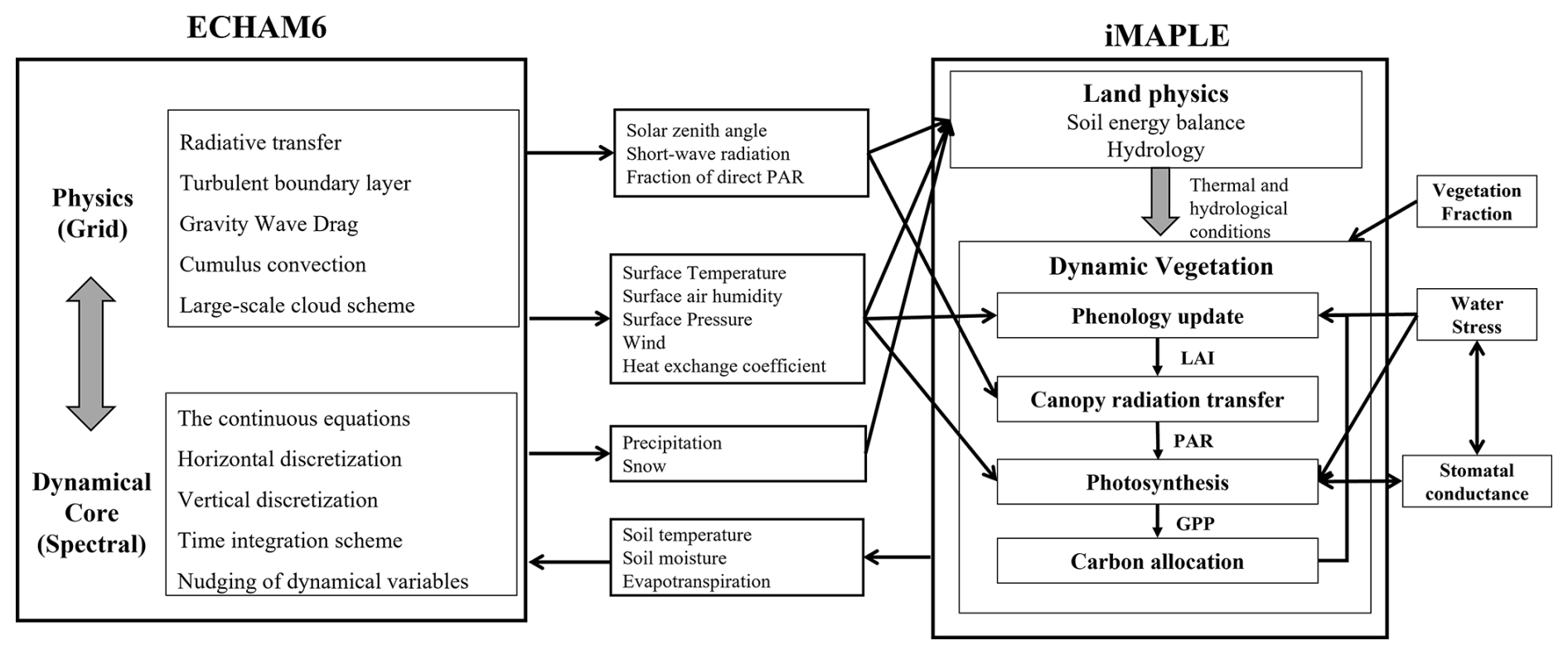
Figure 1 The integrated modeling framework for ECHAM6-iMAPLE v1.0: Atmosphere–Ecosystem Coupled Model. Left: ECHAM6 atmospheric processes. Centre: land–atmosphere coupling interface. Right: iMAPLE vegetation and hydrology.

ECHAM6 integrates atmospheric dynamic processes at an interval of 7.5 min, which is much shorter than the 60-minute interval used in iMAPLE. As a result, simulated climatic variables from ECHAM6 are passed to iMAPLE every 8 ECHAM6 time steps. To ensure seamless information exchange, iMAPLE adopts the same core functional modules as ECHAM6 for input/output (I/O) operations, memory management, parallel computation, and calendar handling. At each coupling interval, ECHAM6 provides hourly meteorological variables to iMAPLE, including precipitation, surface air temperature, wind speed, humidity, surface pressure, CO₂ concentrations, direct and total radiation. In return, iMAPLE feeds back simulated soil temperature, soil moisture, and ET to ECHAM6. These variables further change the surface energy and water balance, thereby altering heat and moisture fluxes that define the atmospheric lower boundary conditions and regulate near-surface climate. Land-atmosphere energy exchange is governed by the surface energy balance, which constrains the transfer of energy between the land surface and the atmosphere:

$$\begin{array}{}\text{(15)}& C{\displaystyle \frac{\partial T_{\mathrm{surf}}}{\partial t}}=R_{\mathrm{net}}+H_{\mathrm{sensible}}+H_{\mathrm{latent}}+G\end{array}$$

where T_surf is the surface temperature, C is the heat capacity of topmost soil layer, R_net denotes the net radiation, H_sensible is the sensible heat flux, H_latent is the latent heat flux, G represents the ground heat flux, which is obtained from the soil temperature profile:

$$\begin{array}{}\text{(16)}& G=-{\mathit{\lambda }}_{\mathrm{s}}{\displaystyle \frac{\partial T}{\partial z}}{|}_{Z_{\mathrm{surf}}}\end{array}$$

where λ_s is the soil thermal conductivity and z is the depth. Replacing soil temperature therefore revises the near-surface thermal gradient and G, which in turn shifts the tendency of T_surf and the partitioning of surface energy into sensible heat. The latent heat flux is linked to ET as follows:

$$\begin{array}{}\text{(17)}& H_{\mathrm{latent}}=L\cdot \mathrm{ET}\end{array}$$

where L is the latent heat of vaporization. Replacing ET revises H_latent and affects the surface energy balance. The replacement of near-surface soil moisture updates the land hydrological state, thereby modifying available soil water and regulating subsequent land-atmosphere moisture exchange. The resulting surface heat and moisture fluxes provide the lower boundary conditions for vertical turbulent transport of dry static energy and specific humidity in ECHAM6. Specifically, an implicit surface-atmosphere coupling scheme uses surface dry static energy and saturated surface humidity, constrained by the surface energy balance, as lower boundary conditions, after which the atmospheric column is updated upward from the lowest model level. Consequently, changes in land surface states, including soil temperature, soil moisture, and ET, propagate to near-surface air temperature and humidity, and further influence the atmospheric column through turbulent diffusion. Extensive numerical tests were conducted to ensure integration stability and computational efficiency of the coupled modeling framework.

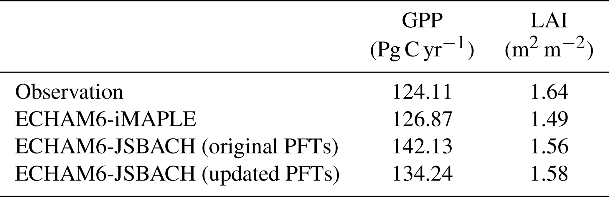
The land cover dataset used in iMAPLE was developed by integrating satellite-based observations from Moderate Resolution Imaging Spectroradiometer (MODIS) and Advanced Very High Resolution Radiometer (AVHRR) (Defries et al., 2000; Hansen et al., 2003), which include nine PFTs representing major global terrestrial ecosystems. In contrast, JSBACH employs a flexible land-cover library that allows users to specify the number and properties of PFTs. To reduce uncertainties arising from differences in boundary conditions, the iMAPLE land cover dataset was harmonized and mapped onto the JSBACH PFT categories (Table 1). Comparisons of simulated GPP and LAI from ECHAM6-JSBACH showed improved performance when using the updated PFT derived from iMAPLE (Table 2). Therefore, this updated land cover configuration of ECHAM6-JSBACH is adopted for subsequent comparison with ECHAM6-iMAPLE. The experiments were driven by observed sea surface temperature and sea ice fraction without atmospheric nudging. The interactive HAM/MOZ chemistry and aerosol modules were disabled. Greenhouse gas concentrations followed the CMIP6 historical pathway. Both ECHAM6-iMAPLE and ECHAM6-JSBACH simulations used identical atmospheric settings at T63L47 resolution for the period of 2000–2014. The first five years were used for model spin-up, and the remaining 10 years were averaged for analysis and performance assessment.

Table 1 Projection of PFTs from JSBACH to iMAPLE.

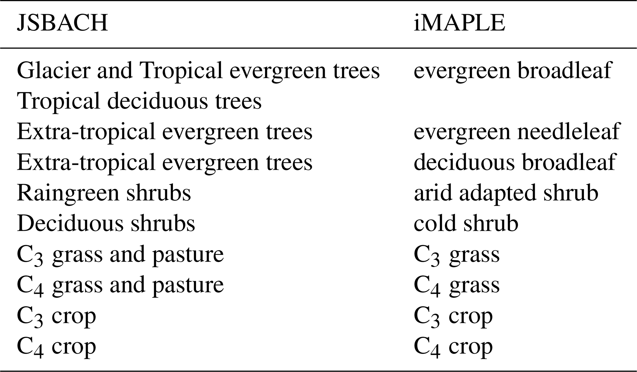
Table 2 Comparison of Gross Primary Productivity (GPP) and Leaf Area Index (LAI) between observational datasets and simulations from ECHAM6-iMAPLE and ECHAM6-JSBACH with original/updated PFTs.

2.4 Data for model evaluations

Observational and reanalysis datasets from 2005 to 2014 were used to evaluate and compare the performance of the ECHAM6-iMAPLE model and ECHAM6-JSBACH models. Specifically, Global LAnd Surface Satellite (GLASS) products were used to assess LAI. For GPP and ET, we used the benchmark product of FLUXCOM datasets (Tramontana et al., 2016; Jung et al., 2020), which generate global gridded flux estimates using machine learning algorithms trained on flux measurements from FLUXNET eddy covariance sites. We also used the Modern-Era Retrospective analysis for Research and Applications, Version 2 (MERRA-2) product (Gelaro et al., 2017) for the evaluations of soil temperature, soil moisture, surface air temperature, and precipitation. Near-surface soil moisture was derived from the MERRA-2 surface wetness variable GWETTOP, which represents relative saturation in the topmost soil layer. GWETTOP was converted to volumetric water content (m³ m⁻³) by multiplying it by the grid-cell soil porosity. All datasets were interpolated to the T63 spectral resolution for consistent comparisons, corresponding to a horizontal resolution of approximately 1.875° in both latitude and longitude.

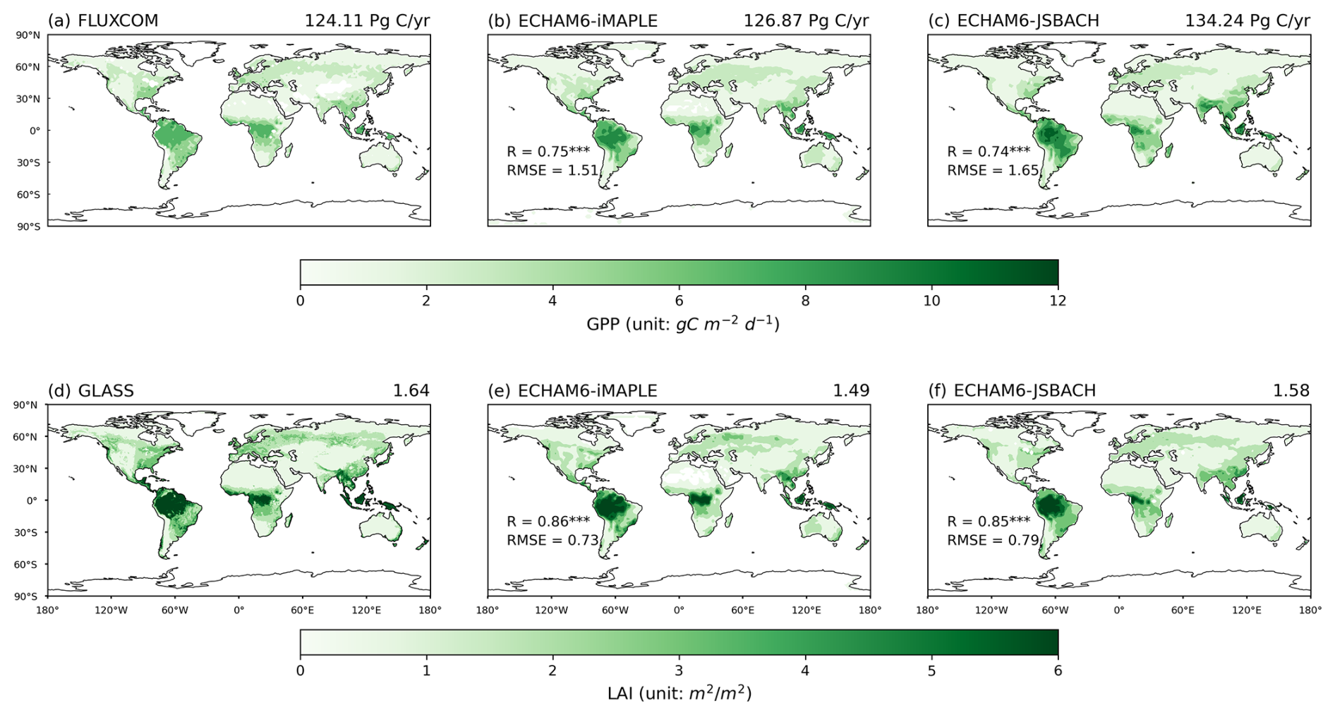
Figure 2 Spatial distributions of (a) gross primary productivity (GPP, g C m⁻² d⁻¹) from FLUXCOM and (d) leaf area index (LAI, m² m⁻²) from GLASS, compared with simulations from (b, e) ECHAM6-iMAPLE and (c, f) ECHAM6-JSBACH. Both model simulations and benchmark/observational datasets are averaged for the period of 2005–2014. The spatial correlation coefficient (R) and root mean square error (RMSE) between simulations and the corresponding observations are shown in the lower left corner of the simulation panels.

3 Results

3.1 Terrestrial carbon cycle

We evaluated the performance of ECHAM6-iMAPLE and ECHAM6-JSBACH in simulating terrestrial carbon fluxes (Fig. 2). Both models reasonably capture the spatial distribution of GPP consistent with FLUXCOM observations, characterized by high values in tropical regions, moderate values in boreal forests, and low values in arid areas. ECHAM6-iMAPLE simulates a global annual total GPP of 126.9 Pg C yr⁻¹, slightly higher than that of 124.1 Pg C yr⁻¹ estimated by the FLUXCOM benchmark. In contrast, ECHAM6-JSBACH produces a much higher global GPP of 134.2 Pg C yr⁻¹, with pronounced positive biases mainly over tropical forest regions, including the Indian subcontinent, the Amazon Basin, and Central Africa (Fig. 2c). Relative to ECHAM6-JSBACH, ECHAM6-iMAPLE exhibits improved performance (Fig. 2b), reflected by a higher correlation coefficient (R=0.75, p<0.01) and a lower root mean square error (RMSE = 1.51 g C m⁻² d⁻¹). This improvement can be primarily attributed to the calibration of vegetation photosynthetic parameters in iMAPLE based on site-level datasets (Yue and Unger, 2015), as well as the constraint of plant phenology through satellite-based observations (Yue et al., 2015).

Consistent with the GPP pattern, simulated LAI from ECHAM6-iMAPLE (Fig. 2e) shows a higher R of 0.86 (p<0.01) and a lower RMSE of 0.73 m² m⁻² against GLASS retrievals (Fig. 2d) compared to ECHAM6-JSBACH (Fig. 2f). Regionally, ECHAM6-iMAPLE successfully reproduces the elevated LAI in tropical rainforests, in good agreement with observational patterns. Globally, ECHAM6-iMAPLE underestimates LAI by about 9 %, primarily due to notable underestimation across high-latitude regions of the Northern Hemisphere (Fig. 2e). In contrast, ECHAM6-JSBACH shows a higher RMSE of 0.79 relative to GLASS, with the largest negative biases occurring in the central Africa and the Southeast Asia region (Fig. 2f).

3.2 Terrestrial water flux

We evaluated the simulated water fluxes from ECHAM6-iMAPLE and ECHAM6-JSBACH (Fig. 3). Both models successfully reproduce the observed ET patterns, characterized by hotspots over tropical rainforest and low values in arid and/or cold regions. Simulated ET from ECHAM6-iMAPLE (Fig. 3b) exhibits a higher spatial correlation with the FLUXCOM benchmark (Fig. 3a) (R=0.86, p<0.01) and a lower RMSE (15.2 mm per month) compared to ECHAM6-JSBACH (Fig. 3c). Globally, the area-weighted mean ET simulated by ECHAM6-iMAPLE is 45.5 mm per month, closely matching the observed value of 45.9 mm per month, whereas ECHAM6-JSBACH underestimates ET at 42.1 mm per month. The poorer performance of ECHAM6-JSBACH is mainly attributed to substantial underestimations in arid and semi-arid regions, particularly over the western United States and Australia (Fig. 3c).

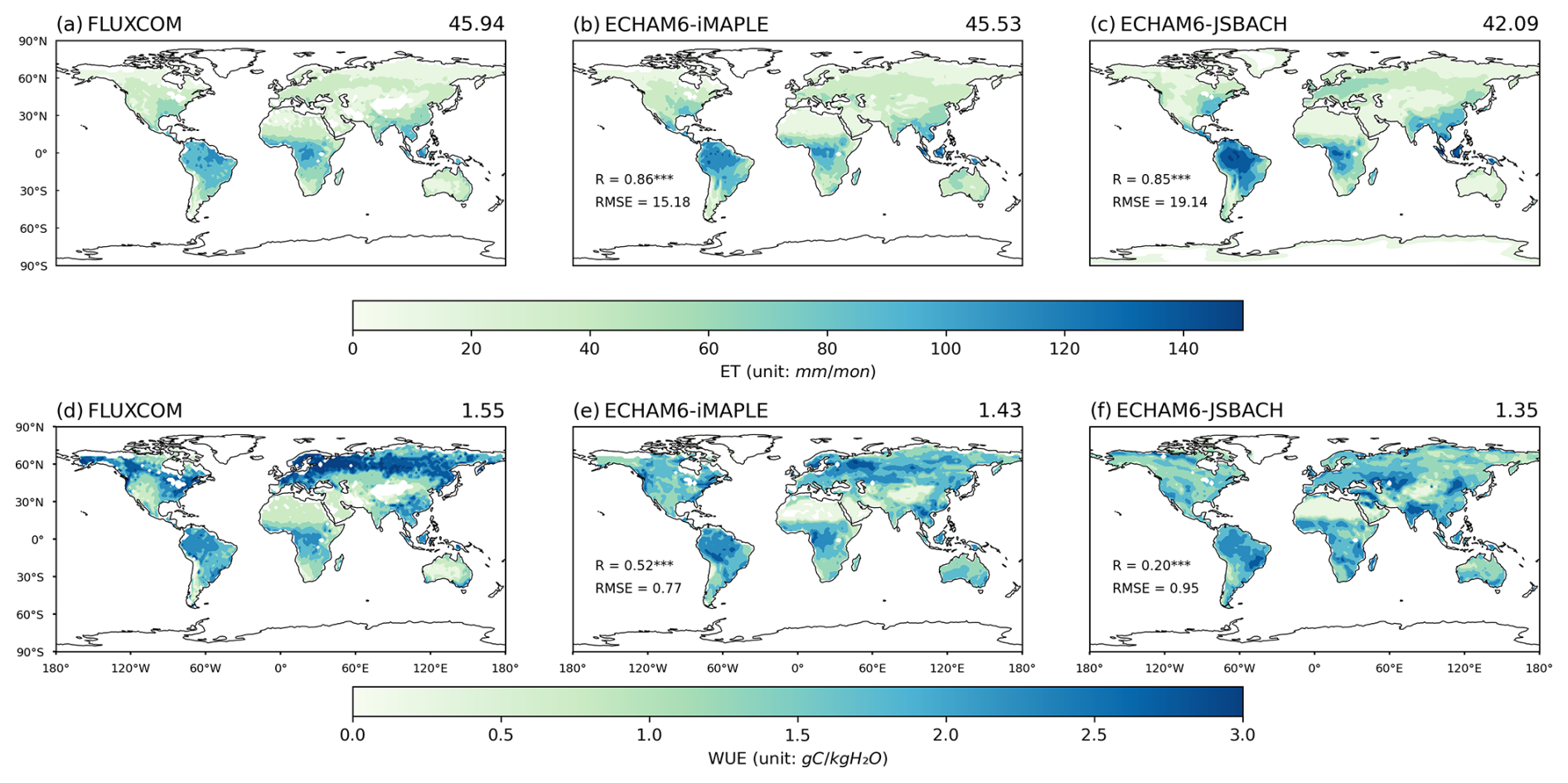
Figure 3 Spatial distributions of (a) evapotranspiration (ET, mm per month) and (d) water use efficiency (WUE, g C kg⁻¹ H₂O) from FLUXCOM, compared with simulations from (b, e) ECHAM6-iMAPLE and (c, f) ECHAM6-JSBACH. Both model simulations and the FLUXCOM benchmark datasets are averaged for the period of 2005–2014. The spatial R and RMSE between simulations and benchmark are shown in the lower left corner of simulation panels. The area-weighted mean ET and WUE are indicated at the top of each panel.

For water use efficiency (WUE), defined as the ratio of GPP to ET, ECHAM6-iMAPLE exhibits high values in the northern middle-to-high latitudes and moderate values in the tropics (Fig. 3e). It achieves a spatial R of 0.52 (p<0.01) and an RMSE of 0.77 g C kg⁻¹ H₂O against the FLUXCOM benchmark (Fig. 3d). In contrast, ECHAM6-JSBACH exhibits substantially poorer performance, with a lower spatial R of 0.20 and a higher RMSE of 0.95 g C kg⁻¹ H₂O (Fig. 3f), which is primarily associated with underestimated ET across mid-to-high northern latitudes and Central Africa. At the global scale, the area-weighted mean WUE simulated by ECHAM6-iMAPLE is 1.43 g C kg⁻¹ H₂O, closer to the FLUXCOM estimate of 1.55 g C kg⁻¹ H₂O and representing a clear improvement over the 1.35 g C kg⁻¹ H₂O simulated by ECHAM6-JSBACH (Fig. 3f).

3.3 Seasonal variations

In addition to the spatial pattern, ECHAM6-iMAPLE effectively captures the seasonal cycles of terrestrial carbon and water fluxes (Fig. 4). Consistent with observations, simulated GPP and ET both reach their annual maxima during the vegetation growing season, with the most pronounced peak occurring in July (Fig. 4a and c). Although the LAI simulated by ECHAM6-iMAPLE exhibits a one-month lag relative to the observations, the temporal correlation remains high (R=0.96), indicating a good representation of seasonal dynamics (Fig. 4b). In contrast, ECHAM6-JSBACH predicts the annual peaks of terrestrial carbon and water fluxes in June, one month earlier than observed peaks. Moreover, the corresponding R between ECHAM6-JSBACH simulations and observations are consistently lower than those derived from ECHAM6-iMAPLE (Fig. 4). The divergence in peak timing and the systematically lower R values collectively demonstrate that ECHAM6-iMAPLE provides a more accurate representation of the seasonal dynamics of terrestrial carbon and water cycle processes compared to ECHAM6-JSBACH.

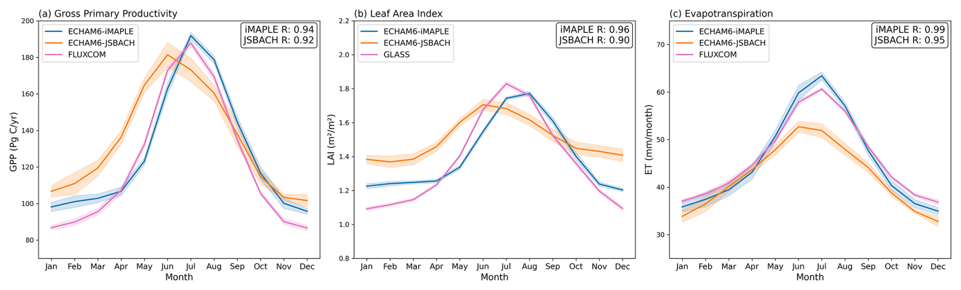
Figure 4 Comparison of the seasonal cycle of (a) GPP (Pg C yr⁻¹), (b) LAI (m² m⁻²), (c) ET (mm per month). The pink lines represent observational or benchmark datasets. The blue and orange lines represent simulations from the ECHAM6-iMAPLE and ECHAM6-JSBACH models, respectively. The shaded areas indicate the interannual variability (one standard deviation) over the period 2005–2014.

3.4 Soil properties and near-surface climate

Soil temperature and moisture play critical roles in regulating vegetation growth (Davidson and Janssens, 2006; Green et al., 2019). Both ECHAM6-iMAPLE (Fig. 5b) and ECHAM6-JSBACH (Fig. 5c) predict high soil temperatures in tropical regions, especially in northern Africa and the Indian Peninsula. The two models exhibit extremely high spatial correlations with MERRA-2 reanalysis data (R=0.99 and 0.98, respectively). However, ECHAM6-iMAPLE more accurately reproduces the global mean soil temperature and shows a lower RMSE of 2.16 K, whereas ECHAM6-JSBACH shows a slight warm bias with a higher RMSE of 2.49 K. For soil moisture, ECHAM6-JSBACH shows substantial overestimation in tropical regions and the high-latitude Northern Hemisphere, leading to a 39.1 % overestimation of the global mean value compared to MERRA-2 (Fig. 5f). In contrast, ECHAM6-iMAPLE closely matches the global mean soil moisture from MERRA-2, with a lower RMSE of 0.07 and a moderate spatial R of 0.76 (Fig. 5e).

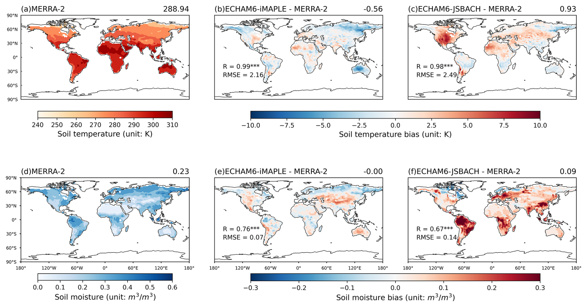
Figure 5 Spatial distributions of (a) soil temperature (ST, K) and (d) near-surface soil moisture (SM, m³ m⁻³) from MERRA-2 reanalyses, biases of (b, e) ECHAM6-iMAPLE and (c, f) ECHAM6-JSBACH relative to MERRA-2. Both model simulations and MERRA-2 reanalyses are averaged for the period of 2005–2014. The spatial R and RMSE between simulations and reanalyses are shown in the lower left corner of simulation panels. The area-weighted mean (or mean biases) ST and SM are indicated at the top of each panel.

Changes in soil temperature and moisture influence surface meteorology through land-atmosphere coupling processes (Seneviratne et al., 2006). We therefore compared surface air temperature and precipitation simulated by ECHAM6-iMAPLE and ECHAM6-JSBACH (Fig. 6). Both models reproduce the large-scale spatial distribution of surface air temperature, albeit with overall warm biases (Fig. 6b and c). However, ECHAM6-iMAPLE performs better than ECHAM6-JSBACH, showing a smaller global mean warm bias (0.34 °C vs. 0.76 °C) and a lower RMSE (3.33 °C vs. 3.47 °C). This improvement is likely associated with the more accurate simulation of soil temperature in ECHAM6-iMAPLE (Fig. 5b), highlighting the role of land surface processes in constraining near-surface climate. For precipitation, however, both models substantially overestimate the global mean amount with regional overestimation in Asia but underestimation in central Africa (Fig. 6e and f). Although coupling with iMAPLE improves the simulation of ET (Fig. 3b) and soil moisture (Fig. 5e), the complex and nonlinear feedbacks within the hydrological cycle may instead magnify biases in precipitation estimates.

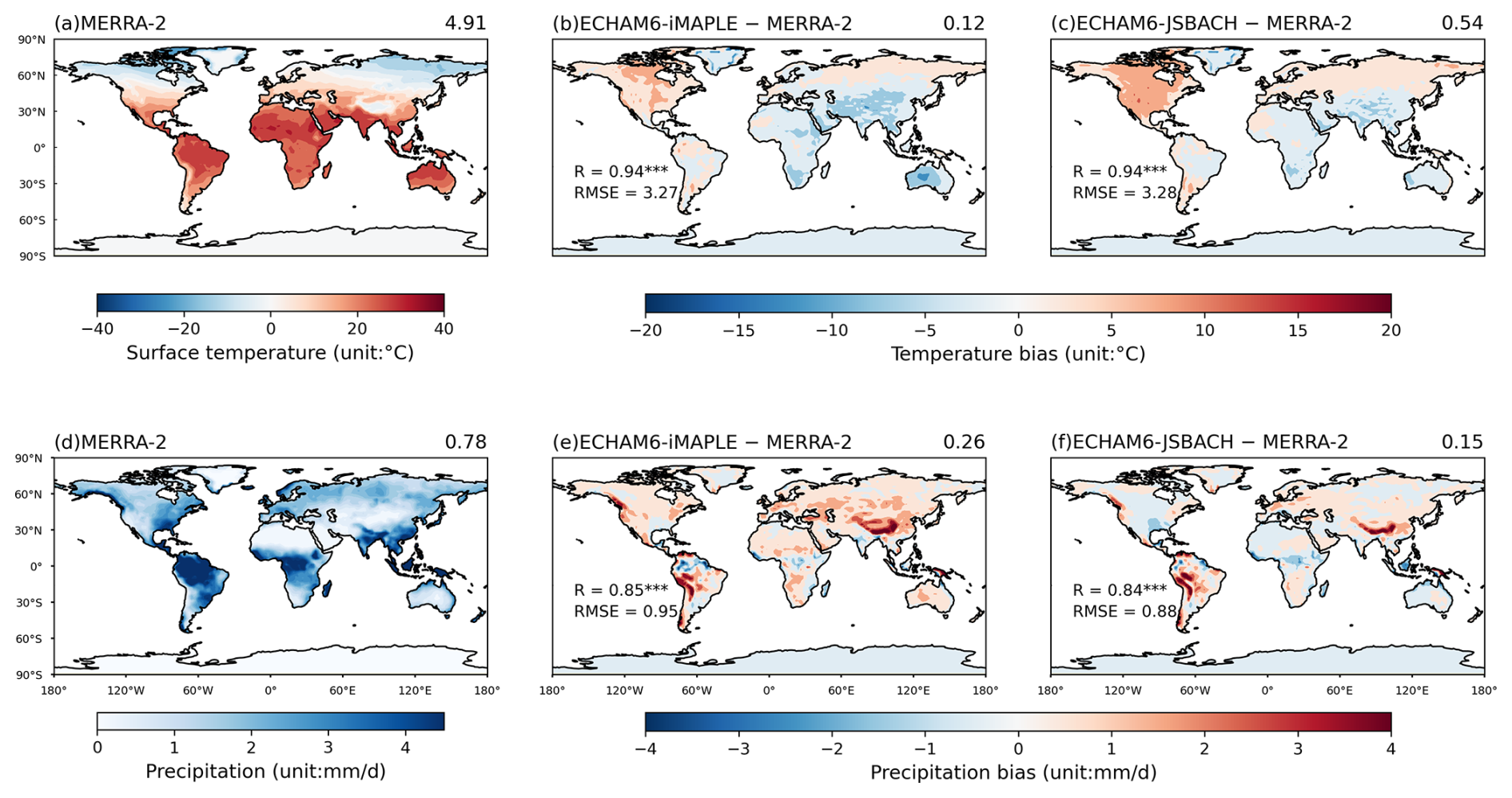
Figure 6 Spatial distributions of (a) surface temperature (T, °C) and (d) precipitation (PREC, mm d⁻¹) from MERRA-2 reanalyses, biases of (b, e) ECHAM6-iMAPLE and (c, f) ECHAM6-JSBACH relative to MERRA-2. Both model simulations and MERRA-2 reanalyses are averaged for the period of 2005–2014. The spatial R and RMSE between simulations and observations are shown in the lower left corner of simulation panels. The area-weighted mean (or mean biases) T and PREC are indicated at the top of each panel.

4 Conclusion and discussion

The terrestrial biosphere and atmosphere are tightly coupled through exchanges of energy, water, carbon, and reactive species (Green et al., 2017). These interactions regulate climate variability, ecosystem resilience, and air pollutants such as ozone and aerosols (Zeng et al., 1999; Yue and Unger, 2014; Zhou et al., 2024). However, climate models often incompletely represent vegetation biophysical and physiological processes, leading to biased carbon and water fluxes and increased uncertainties in weather predictions (Koster et al., 2011; Guo et al., 2012). To address this limitation, we coupled the iMAPLE vegetation model to the ECHAM6 atmospheric general circulation model, and evaluated its performance against reanalysis, benchmark, and satellite datasets. Compared to the original ECHAM6-JSBACH configuration, the updated ECHAM6-iMAPLE model substantially improves simulations of terrestrial carbon and water fluxes, more accurately capturing their spatial patterns and seasonal variations.

These improvements stem from both rigorous parameter calibration and a more realistic representation of key biophysical processes in iMAPLE. Critical physiological parameters (e.g., V_cmax) are tightly constrained using in situ measurements from 201 FLUXNET sites (Yue et al., 2024), and phenological schemes have been validated against thousands of ground-based records and multiple satellite retrievals (Yue et al., 2015). Moreover, iMAPLE distinguished the biophysical effects of direct and diffuse radiation (Yue and Unger, 2017), allowing improved quantifications of canopy radiation transfer and photosynthetic carbon assimilation dynamics. Unlike JSBACH, which applies a fixed carbon allocation scheme among leaf, wood, and reserve pools, iMAPLE adopts a dynamic framework that allocates carbon to root, stem, and leaf respiration in proportion to realistic LAI variations. Together, these advances enhance the ability of ECHAM6-iMAPLE in simulating vegetation dynamics under climate change.

Despite these advances, several limitations remain in the current version of ECHAM6-iMAPLE. First, iMAPLE does not include dynamic nitrogen and phosphorus cycles, introducing uncertainties in simulated photosynthetic responses to elevated CO₂ (Gruber and Galloway, 2008; Zaehle et al., 2011). Second, the vegetation model prescribes land cover and neglects competitions among PFTs, preventing simulation of vegetation shifts under anthropogenic or natural disturbances. Third, not all vegetation properties simulated by iMAPLE are fully coupled to ECHAM6. For instance, dynamically simulated LAI is not consistently used by ECHAM6 to update land surface parameters or ecosystem emissions. In addition, iMAPLE considers the variations of soil temperature and soil moisture only within upper two meters, limiting the full prediction of deeper soil processes in the coupled system.

In future work, we will further improve ECHAM6-iMAPLE in several key aspects. First, incorporating a process-based nitrogen cycle will substantially improve simulations of terrestrial carbon sinks and reduce uncertainties in carbon flux estimates. Second, we will strengthen the representation of natural source and sink processes. A major advantage of iMAPLE lies in its dynamic simulation of natural emissions, including wildfires, biogenic volatile organic compounds (BVOCs), and soil emissions. In addition, dynamically simulated stomatal conductance influences the dry deposition of atmospheric constituents. Future efforts will focus on improving the real-time simulation and evaluation of these source-sink processes within the coupled framework. Third, we plan to incorporate an interactive module of atmospheric chemistry into ECHAM6-iMAPLE to enable fully coupled interactions among climate, ecosystems, and atmospheric chemistry. This development will enhance capabilities for climate projection and air pollution forecasting, and provide a useful tool for quantifying the long-term impacts of human activities on the Earth system through multi-sphere interactions and feedbacks.