A hybrid method for winter road surface temperature prediction using improved LSTMs and stacking-based ensemble learning

Accurate prediction of road surface temperature (RST) is essential for proactive winter road maintenance and traffic safety management. However, existing approaches – ranging from physics-based models to data-driven methods – either require detailed pavement thermal parameters that are rarely available at operational road meteorological stations, or lack the capacity to simultaneously exploit local meteorological analogues and long-range temporal dependencies in an interpretable ensemble framework. This study proposes the Improved LSTMs Ensemble with Stacking (ILES) framework, which integrates two base learners with partially complementary predictive characteristics within a stacking ensemble employing out-of-fold cross-validation. The first base learner, KNN-LSTM, augments sequential modelling with similarity-based retrieval of historically analogous meteorological states to capture locally recurrent patterns. The second, BiLSTM-MHA, combines bidirectional recurrent processing with multi-head self-attention to extract long-range temporal dependencies across a 24 h input window. Moreover, a Bayesian Ridge Regression meta-learner fuses the base-learner outputs through Evidence Maximization, yielding probabilistic forecasts with closed-form posterior predictive uncertainty at the ensemble combination layer. The framework is trained and evaluated on four consecutive winter seasons (December 2020 to February 2024) of road meteorological observations from station M9393 in the northwest inland plain of Jiangsu Province, China. Results indicate that ILES achieves lower prediction errors in general than ten other models spanning persistence forecasting, traditional machine learning, and deep learning approaches, with R² reaching 0.993, 0.923, and 0.826 at 1, 3, and 6 h forecasting horizons, respectively. Among three input configurations evaluated, physics-motivated feature engineering incorporating the air–surface temperature gradient and multi-scale RST temporal tendencies outperforms both the station-only baseline and ERA5-Land reanalysis augmentation, indicating that domain-knowledge-guided feature construction provides a more effective and operationally practical input strategy at instrumented sites. SHAP-based interpretability analysis, stratified by temperature regime and diurnal cycle, confirms that the learned feature importance rankings are qualitatively consistent with the dominant drivers of RST evolution identified by surface energy balance theory. Multi-site generalization is further validated at two independent stations within the same temperate monsoon climate zone, confirming the transferability of the proposed framework across different road environments within this climate setting.

1 Introduction

Accurate prediction of road surface temperature (RST) is a prerequisite for effective winter road maintenance and traffic-safety management (Shao and Lister, 1996; Nantasai and Nassiri, 2019; Zhao et al., 2020). Sub-zero pavement temperatures substantially reduce the pavement friction coefficient, increasing the risk of vehicle accidents and network-wide congestion. Because RST governs the phase state of moisture at the pavement-atmosphere interface, it serves as the primary indicator for determining whether wet road surfaces will freeze under prevailing meteorological conditions (Li et al., 2022; Nowrin and Kwon, 2022; Zhang et al., 2023).

From a physical standpoint, RST is governed by the surface energy balance (SEB) at the pavement–atmosphere interface. Following Hermansson (2004) and Chen et al. (2019), the net energy flux at the road surface can be expressed as:

$$\begin{array}{}\text{(1)}& Q^{*}=Q_{\mathrm{h}}+Q_e+Q_{\mathrm{G}}+Q_{\mathrm{m}},\end{array}$$

where Q^* is the net radiation flux; Q_h is the turbulent sensible heat flux driven by the surface–air temperature gradient and wind speed; Q_e is the latent heat flux modulated by relative humidity and precipitation; Q_G is the pavement heat storage flux governed by the substrate's thermal conductivity and heat capacity; and Q_m represents the latent heat of fusion associated with freezing or melting of surface moisture. All flux terms adopt a sign convention in which positive values denote energy directed into the road surface and negative values denote energy loss from the surface; under this convention, Q^* represents the net radiative energy available to drive the remaining flux terms. RST reflects the cumulative outcome of these fluxes over preceding hours, exhibiting diurnal periodicity, lagged responses to radiative forcing, and abrupt thermal transitions during precipitation events or cold-air advection (Hermansson, 2004; Chen et al., 2019). This physical understanding motivates both the selection of meteorological predictors and the design of derived input features in the present study.

RST prediction presents two fundamental challenges that existing approaches have not simultaneously resolved. Physics-based models – including finite-difference, finite-element, and finite-volume formulations – solve the surface energy balance equation coupled to one-dimensional heat conduction in the pavement substrate and can yield physically interpretable, high-accuracy solutions when site-specific thermal parameters are well characterised (Hermansson, 2004; Wang et al., 2009; Chen et al., 2019; Minhoto et al., 2005; Schindler et al., 2004; Saliko et al., 2023). However, their accuracy is critically sensitive to pavement thermal and radiative properties – thermal conductivity, volumetric heat capacity, surface emissivity, and the convective heat transfer coefficient – that are rarely available at operational road meteorological stations (Qin and Hiller, 2013; Athukorallage et al., 2023; Ayasrah et al., 2023; Adwan et al., 2021). This parameter identifiability constraint extends to operational systems such as METRo (Crevier and Delage, 2001), whose performance remains dependent on accurate specification of pavement layer properties, surface albedo, and anthropogenic heat sources that vary across road segments and degrade over time (Shao and Lister, 1996; Kangas et al., 2015; Karsisto et al., 2016), fundamentally limiting the scalability of physics-based approaches to the large number of heterogeneous road segments for which detailed subsurface characterisation is unavailable. Concurrently, RST is a strongly autocorrelated variable whose evolution reflects the integrated effect of meteorological forcing over preceding hours, exhibiting lagged responses to radiative and turbulent fluxes and regime-dependent nonlinear dynamics during precipitation events or nocturnal radiative cooling. Statistical and empirical models – including multiple linear regression, stepwise regression, and regression-based nowcast systems – have identified near-surface air temperature and lagged RST as the dominant predictors (Yin et al., 2019; Kršmanc et al., 2013; Li et al., 2018; Diefenderfer et al., 2006; Asefzadeh et al., 2017; Hassan et al., 2005), yet these approaches impose linearity or low-order polynomial constraints on the inherently nonlinear meteorology–RST relationship, precluding adequate representation of the multi-hour temporal dependencies and abrupt thermal transitions that characterise real-world RST evolution (Wang, 2015; Gedafa et al., 2014; Darghiasi et al., 2025; Jing and Zhang, 2018).

Data-driven machine learning (ML) methods address the nonlinearity limitation by learning flexible input–output mappings directly from observational records without requiring explicit thermal parameter calibration. Ensemble tree methods, including random forest (RF), gradient boosting decision trees (GBDT), and extreme gradient boosting (XGBoost), have achieved strong predictive performance by aggregating predictions from multiple weak learners (Milad et al., 2021b; Qiu et al., 2020; Liu et al., 2018; Kebede et al., 2024; Yuan et al., 2025). Support vector regression (SVR) and Gaussian process regression (GPR) have captured nonlinear RST–meteorology relationships under varying surface conditions (Molavi Nojumi et al., 2022; Wang et al., 2023), and artificial neural networks (ANNs) have demonstrated superior pattern-learning capacity relative to conventional regression approaches (Abo-Hashema, 2013; Rigabadi et al., 2022). However, these methods treat each input sample independently and therefore cannot exploit the multi-hour temporal autocorrelation structure inherent in RST time series, constraining their ability to represent the thermal inertia and lag dynamics that are characteristic of RST evolution (Yang et al., 2020; Hatamzad et al., 2022; Darghiasi et al., 2024).

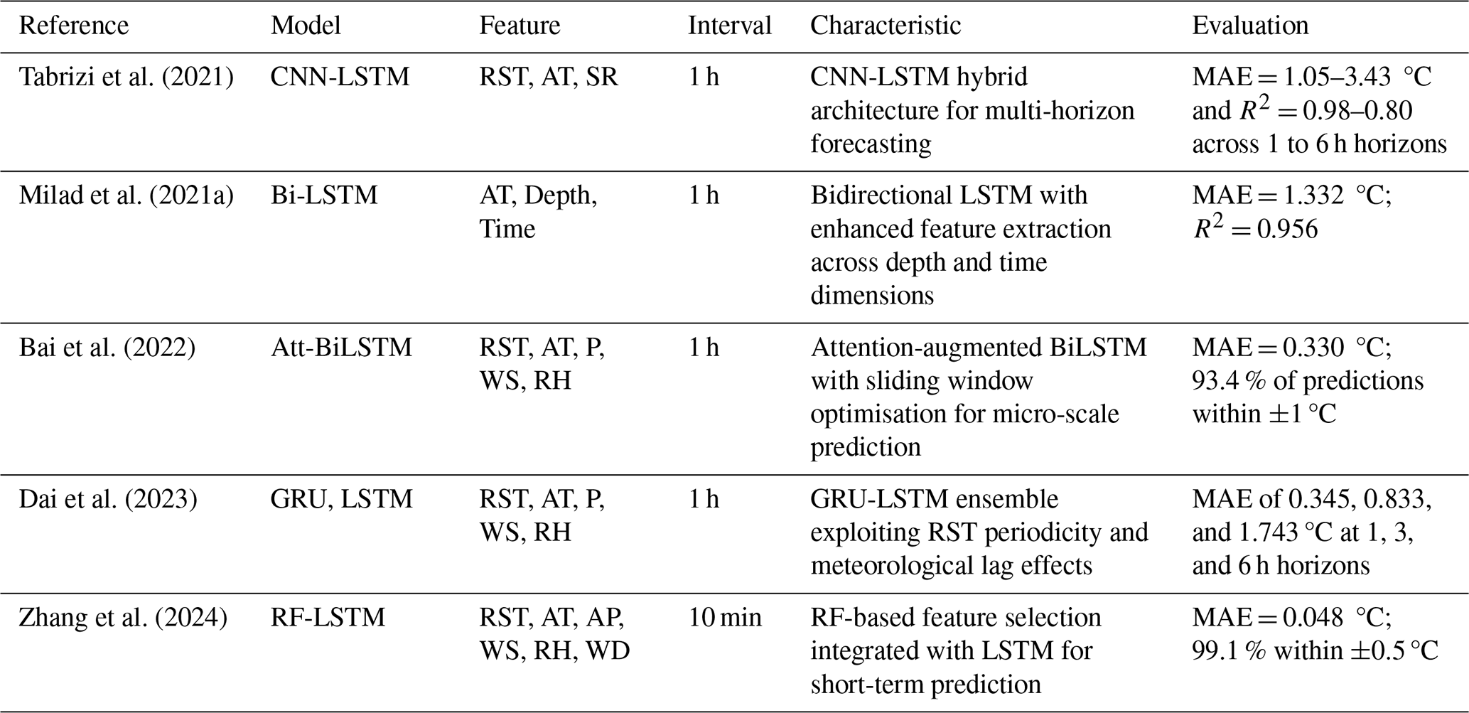
Recurrent deep learning architectures, and in particular Long Short-Term Memory (LSTM) networks and their variants, address this limitation more directly by learning sequential dependencies through gating mechanisms that selectively retain and discard information over multi-hour input windows (Dai et al., 2023; Ghalandari et al., 2023). Several studies have demonstrated their superiority over traditional ML approaches for RST prediction: Tabrizi et al. (2021) showed that a hybrid CNN-LSTM model outperformed LSTM, ConvLSTM, Seq2Seq, and WaveNet baselines across 1, 2, 4, and 6 h horizons; Zhang et al. (2023) reported MAE of 0.82 °C and RMSE of 1.24 °C with an XGBoost-LSTNet combination; Li et al. (2022) showed that a hybrid Bayesian structural time series-Bayesian neural network model attained greater than 95 % coverage within predicted confidence intervals; Dai et al. (2023) proposed a GRU-LSTM ensemble exploiting RST periodicity and meteorological lag effects; and Zhang et al. (2024) integrated RF-based feature selection with LSTM for short-term prediction at 10 min resolution. Bidirectional LSTM (BiLSTM) architectures, which process the input sequence in both forward and backward temporal directions, have shown enhanced feature-extraction capabilities relative to unidirectional LSTMs (Maddu et al., 2021; Tao et al., 2024; Milad et al., 2021a). Bai et al. (2022) demonstrated that an attention-based Bi-LSTM achieved 93.4 % of predictions within 1 °C error. Table 1 summarizes recent LSTM-based approaches for RST prediction, including the model architectures employed, the input features considered, and representative predictive accuracy reported in each study.

Table 1 Summary of LSTM-based approaches for road surface temperature prediction. The accuracy values reported in Table 1 are drawn from the original publications and reflect different datasets, input variables, temporal resolutions, and evaluation protocols, they are presented here for literature-positioning purposes only. Abbreviations: AT, air temperature; SR, solar radiation; RH, relative humidity; P, precipitation; WS, wind speed; WD, wind direction; AP, atmospheric pressure; Depth, measurement depth below pavement surface; Time, time-of-day index.

Despite these advances, the existing literature exhibits several limitations that warrant further investigation. First, individual LSTM-based architectures tend to emphasise either local pattern recurrence associated with historically similar meteorological trajectories or long-range temporal dependencies spanning the full input window, but rarely capture both simultaneously. While some studies have explored ensemble combinations of heterogeneous models, the systematic integration of architecturally complementary LSTM variants through principled meta-learning remains underexplored for RST prediction. Moreover, the consistency of ensemble-derived predictive gains across multiple forecasting horizons has not been thoroughly demonstrated. Second, the relative contribution of different input data sources to RST prediction accuracy remains insufficiently characterised. While several studies have incorporated reanalysis products or derived meteorological variables alongside station observations, systematic comparisons across input configurations under consistent experimental conditions are scarce, making it difficult to determine whether the additional data complexity is justified by commensurate predictive gains. Third, although post-hoc feature attribution methods such as SHAP (SHapley Additive exPlanations; Lundberg and Lee, 2017) have been applied to data-driven RST models, existing analyses have typically reported globally averaged attribution values without systematic stratification by temperature regime or time of day. Such stratified analysis would provide a more rigorous basis for evaluating whether learned model behaviour is qualitatively consistent with the dominant meteorological drivers identified by SEB theory, and for identifying conditions under which the model may be less reliable.

Motivated by these limitations, this study proposes the Improved LSTMs Ensemble with Stacking (ILES) framework for winter RST prediction. Rather than relying on a single recurrent architecture, ILES integrates two base learners with partially complementary predictive characteristics – KNN-LSTM for similarity-driven local pattern retrieval and BiLSTM-MHA for long-range temporal dependency extraction – within a stacking ensemble, where a Bayesian Ridge Regression meta-learner fuses the base learner outputs to yield probabilistic forecasts with closed-form posterior predictive uncertainty at the ensemble combination layer; the ablation analysis shows that the combined gain from these two components is sub-additive. Three input configurations – a station-only baseline, ERA5-Land reanalysis augmentation, and physics-motivated feature engineering – are systematically compared to determine the most effective and operationally practical input strategy. In addition, SHAP-based attribution analysis is conducted in a stratified manner across temperature regimes and diurnal cycles, providing a more systematic evaluation of whether learned feature importance is consistent with the dominant drivers identified by SEB theory. The framework is trained and evaluated on four consecutive winter seasons of hourly road meteorological observations from station M9393, located in the northwest inland plain of Jiangsu Province, China, with multi-site generalisation assessed at two independent stations M9474 and M9448.

The remainder of this paper is organized as follows. Section 2 describes the ILES framework, including the KNN-LSTM and BiLSTM-MHA architectures, the stacking ensemble construction, and the Bayesian Ridge Regression meta-learner. Section 3 presents the study site, observational dataset, ERA5-Land reanalysis data, feature engineering procedure, and experimental design. Section 4 reports results encompassing overall predictive performance, input configuration comparisons, ensemble complementarity analysis, and uncertainty quantification. Section 5 summarizes the principal conclusions.

2 Methodology

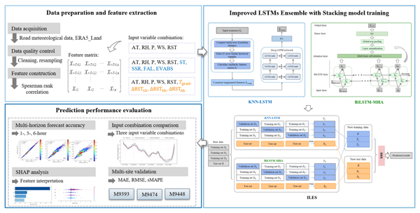
Figure 1 presents an overview of the ILES framework for winter RST prediction, organised into three sequential stages: data preparation and feature extraction, model training and ensemble construction, and prediction performance evaluation.

Figure 1 Overview of the ILES model for winter RST prediction.

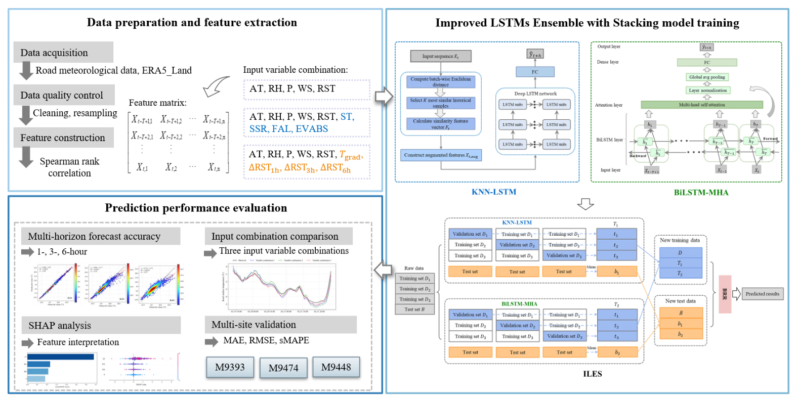
In the first stage, historical meteorological observations from station M9393 and ERA5-Land reanalysis variables are subjected to quality control procedures including outlier removal, missing value imputation, and hourly resampling. Input variables are selected on the basis of Spearman rank correlation with winter RST, and the retained variables are standardised using Z-score normalisation parameters estimated exclusively from the training set. A sliding window is applied to construct sequential input samples across three candidate input configurations, enabling the model to capture the multi-hour autocorrelation structure and diurnal periodicity inherent in RST time series.

In the second stage, two structurally distinct LSTM variants serve as base learners within a stacking ensemble. KNN-LSTM augments temporal sequence modelling with similarity-based feature retrieval from historical analogues, enabling the model to leverage locally recurrent meteorological patterns. BiLSTM-MHA employs bidirectional recurrent processing combined with multi-head self-attention to extract long-range temporal dependencies across the full input window. Base learner predictions for the meta-learner training matrix are generated through three-fold temporal cross-validation aligned to complete winter seasons, with each fold corresponding to one complete winter as the validation period. A BRR meta-learner is fitted on the resulting out-of-fold predictions, yielding probabilistic forecasts with closed-form uncertainty quantification as the final ensemble output.

In the third stage, the ILES model is assessed from four analytical perspectives: comprehensive benchmarking against ten models across 1, 3, and 6 h forecasting horizons; comparison of three input variable combinations to evaluate the relative predictive value of station observations, ERA5-Land reanalysis augmentation, and physics-motivated feature engineering; stratified SHAP-based attribution analysis across temperature regimes and diurnal cycles; and multi-site validation at stations with distinct geographical and surface conditions.

2.1 KNN-LSTM

The proposed KNN-LSTM model integrates similarity-based feature augmentation with temporal sequence modelling to improve predictive accuracy for wintertime RST forecasting, building upon the framework established by Luo et al. (2019) for traffic flow prediction.

Consider a forecasting task in which the objective is to predict RST at time t+h from a sliding window of historical observations. Let X_t denote the input feature matrix at time t, of dimension T×n, where T is the window size and n is the feature dimension. Given a training set of M historical samples $\mathit{\left\{}\right({\mathbf{X}}_i,y_i){\mathit{\}}}_{i=\mathrm{1}}^M$, where X_i is the ith input window and y_i is the corresponding target RST, the similarity between a query window X_t and each training sample is measured by Euclidean distance in the flattened feature space. The resulting distance matrix is normalised via min–max scaling to ensure numerical comparability:

$$\begin{array}{}\text{(2)}& {\mathbf{D}}_{\mathrm{norm}}={\displaystyle \frac{\mathbf{D}-min\left(\mathbf{D}\right)}{max\left(\mathbf{D}\right)-min\left(\mathbf{D}\right)+\mathit{ϵ}}},\end{array}$$

where ϵ is a small constant to avoid division by zero. The K nearest neighbours $\mathit{\{}{\mathbf{X}}_{\left(k\right)}{\mathit{\}}}_{k=\mathrm{1}}^K$ are identified as the K reference samples with the smallest normalised distances to X_t. The similarity feature matrix F_t is then constructed as their uniform average:

$$\begin{array}{}\text{(3)}& {\mathbf{F}}_t={\displaystyle \frac{\mathrm{1}}{K}}{\sum }_{k=\mathrm{1}}^K{\mathbf{X}}_{\left(k\right)},\end{array}$$

capturing the central tendency of historically analogous meteorological states. The augmented input is formed by concatenating X_t and F_t along the feature dimension:

$$\begin{array}{}\text{(4)}& {\mathbf{X}}_{t,\mathrm{aug}}=[{\mathbf{X}}_t,{\mathbf{F}}_t].\end{array}$$

This augmentation strategy preserves the original temporal structure while incorporating rich contextual information from analogous meteorological conditions in the historical record, and the dimensionality of the input doubles from n to 2n. The augmented sequence X_t,aug is fed into a three-layer LSTM network (Hochreiter and Schmidhuber, 1997) designed to capture hierarchical temporal dependencies:

$$\begin{array}{}\text{(5)}& {\displaystyle }{\mathit{h}}_{\mathit{\tau }}^{\left(\mathrm{1}\right)},{\mathit{c}}_{\mathit{\tau }}^{\left(\mathrm{1}\right)}={\mathrm{LSTM}}_{\mathrm{1}}\left({\mathbf{X}}_{t,\mathrm{aug}},h_{\mathit{\tau }-\mathrm{1}}^{\left(\mathrm{1}\right)},c_{\mathit{\tau }-\mathrm{1}}^{\left(\mathrm{1}\right)};{\mathit{\theta }}_{\mathrm{1}}\right),\text{(6)}& {\displaystyle }{\mathit{h}}_{\mathit{\tau }}^{\left(\mathrm{2}\right)},{\mathit{c}}_{\mathit{\tau }}^{\left(\mathrm{2}\right)}={\mathrm{LSTM}}_{\mathrm{2}}\left({\mathit{h}}_{\mathit{\tau }}^{\left(\mathrm{1}\right)},h_{\mathit{\tau }-\mathrm{1}}^{\left(\mathrm{2}\right)},c_{\mathit{\tau }-\mathrm{1}}^{\left(\mathrm{2}\right)};{\mathit{\theta }}_{\mathrm{2}}\right),\text{(7)}& {\displaystyle }{\mathit{h}}_{\mathit{\tau }}^{\left(\mathrm{3}\right)},{\mathit{c}}_{\mathit{\tau }}^{\left(\mathrm{3}\right)}={\mathrm{LSTM}}_{\mathrm{3}}\left({\mathit{h}}_{\mathit{\tau }}^{\left(\mathrm{2}\right)},h_{\mathit{\tau }-\mathrm{1}}^{\left(\mathrm{3}\right)},c_{\mathit{\tau }-\mathrm{1}}^{\left(\mathrm{3}\right)};{\mathit{\theta }}_{\mathrm{3}}\right),\end{array}$$

where ${\mathit{h}}_{\mathit{\tau }}^{\left(\mathrm{\ell }\right)}$ and ${\mathit{c}}_{\mathit{\tau }}^{\left(\mathrm{\ell }\right)}$ denote the hidden state and cell state at layer ℓ and time step τ, respectively, and θ_ℓ represents the learnable parameters. The final hidden state ${\mathit{h}}_T^{\left(\mathrm{3}\right)}$ is passed through a fully connected layer to generate the prediction:

$$\begin{array}{}\text{(8)}& {\widehat{y}}_{t+h}={\mathbf{W}}_{\mathrm{0}}\cdot {\mathit{h}}_T^{\left(\mathrm{3}\right)}+b_{\mathrm{0}},\end{array}$$

where W₀ and b₀ are the learnable weight matrix and bias term, respectively. A separate instance of this model, with independently optimised parameters ${\mathit{\theta }}_{\mathrm{1}},{\mathit{\theta }}_{\mathrm{2}},{\mathit{\theta }}_{\mathrm{3}}$ and W₀,b₀, is trained for each forecasting horizon; no parameters are shared across horizons. A schematic overview of the KNN-LSTM architecture is provided in Figs. 1 and 2.

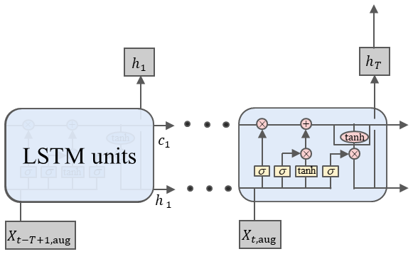
Figure 2 Unrolled computation of a single LSTM layer across the input window, where h_τ and c_τ denote the hidden and cell states at time step τ, with $\mathit{\tau }\in \mathit{\{}\mathrm{1},\mathrm{\dots },T\mathit{\}}$ indexing the steps within the window of length T.

2.2 BiLSTM-MHA

The proposed BiLSTM-MHA model integrates a Bidirectional Long Short-Term Memory network with a multi-head self-attention mechanism (Vaswani et al., 2017), augmented by residual connections and layer normalisation (Ba et al., 2016) to maintain training stability while capturing complex temporal dependencies.

Let the sliding window size be T and the input sequence at time t be $\mathbf{X}=({\mathit{x}}_{t-T+\mathrm{1}},{\mathit{x}}_{t-T+\mathrm{2}},\mathrm{\dots },{\mathit{x}}_t{)}^{\mathrm{\top }}$, where ${\mathbf{x}}_t=(x_{t,\mathrm{1}},x_{t,\mathrm{2}},\mathrm{\dots },x_{t,n}$) and n denotes the feature dimension.

The BiLSTM layer captures temporal dependencies in both temporal directions (Schuster and Paliwal, 1997). At each time step t, the forward LSTM processes the sequence from past to future and the backward LSTM processes the same input sequence in the reverse temporal direction, producing a concatenated hidden state ${\mathit{h}}_t=[{\overrightarrow{\mathit{h}}}_t,{\overleftarrow{\mathit{h}}}_t{]}^{\mathrm{\top }}$, where ${\overrightarrow{\mathit{h}}}_t$ and ${\overleftarrow{\mathit{h}}}_t$ denote the forward and backward hidden states, respectively. The full sequence $H=(h_{\mathrm{1}},h_{\mathrm{2}},\mathrm{\dots },{\mathit{h}}_t$) is passed to the subsequent attention layer. It should be noted that the backward pass operates exclusively within the historical input window $\left[t-T+\mathrm{1},t\right]$ and accesses no observations beyond time t.

The multi-head self-attention mechanism (Vaswani et al., 2017) transforms H through learned linear projections into multiple representation subspaces in parallel, enabling the model to attend simultaneously to different temporal positions and feature abstractions:

$$\begin{array}{}\text{(9)}& \mathrm{MultiHead}\left(\mathbf{Q},\mathbf{K},\mathbf{V}\right)=\mathrm{Concat}\left({\mathrm{head}}_{\mathrm{1}},\mathrm{\cdots },{\mathrm{head}}_{\mathrm{h}}\right){\mathbf{W}}^{\mathrm{O}},\end{array}$$

where each head is defined as head${}_i=\mathrm{Attention}(Q{\mathbf{W}}_i^Q,{\mathbf{KW}}_i^K,{\mathbf{VW}}_i^V$) with Attention$(\mathbf{Q},\mathbf{K},\mathbf{V})=\mathrm{softmax}\left(\frac{{\mathbf{QK}}^{\mathrm{\top }}}{\sqrt{d_{\mathrm{k}}}}\right)\mathbf{V}$. Here W^O denotes the output projection matrix, ${\mathbf{W}}_i^Q$, ${\mathbf{W}}_i^K$, ${\mathbf{W}}_i^V$ are the per-head projection matrices, and d_k is the key dimension. In the self-attention formulation adopted here, Q, K, and V are all derived from H.

A residual connection is applied to the attention output to facilitate gradient flow during backpropagation (He et al., 2016), followed by layer normalisation to stabilise the feature distribution:

$$\begin{array}{}\text{(10)}& {\displaystyle }\mathbf{R}=\mathbf{H}+\mathrm{MultiHead}(\mathbf{H},\mathbf{H},\mathbf{H}),\text{(11)}& {\displaystyle }\mathbf{Z}=\mathrm{LayerNorm}\left(\mathbf{R}\right),\end{array}$$

Temporal aggregation is then performed by global average pooling across all time steps:

$$\begin{array}{}\text{(12)}& \mathit{c}={\displaystyle \frac{\mathrm{1}}{T}}{\sum }_{t=\mathrm{1}}^T{\mathbf{Z}}_t.\end{array}$$

Global average pooling reduces parameter count relative to concatenation-based aggregation and confers robustness to sequence length variation (Lin et al., 2013). The final prediction is generated through a fully connected output layer:

$$\begin{array}{}\text{(13)}& {\widehat{y}}_{t+h}={\mathbf{W}}_{\mathrm{0}}c+b_{\mathrm{0}},\end{array}$$

where W₀ represents the weight matrix and b₀ denotes the bias term. As with KNN-LSTM, a separate instance of the BiLSTM-MHA model – including all BiLSTM, attention, and output-layer parameters – is trained independently for each forecasting horizon, with no weight sharing across horizons. A schematic of the BiLSTM-MHA architecture is provided in Figs. 1 and 3.

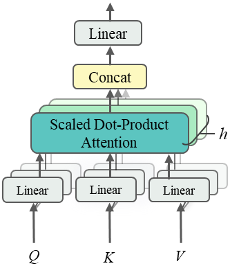
Figure 3 Multi-Head Attention consists of h parallel attention heads, each operating on a distinct learned projection of the input. Q, K, and V are all derived from the BiLSTM output.

2.3 Stacking ensemble with out-of-fold cross-validation

Stacking is a hierarchical ensemble learning method that combines predictions from multiple base learners through a meta-learner to achieve superior predictive performance (Wolpert, 1992; Breiman, 1996). Unlike bagging and boosting, which rely on parallel or sequential resampling strategies, stacking employs a two-layer architecture where diverse base models generate intermediate predictions that are subsequently integrated by a meta-model. This framework has demonstrated remarkable success in time series forecasting tasks by leveraging model complementarity (Divina et al., 2018).

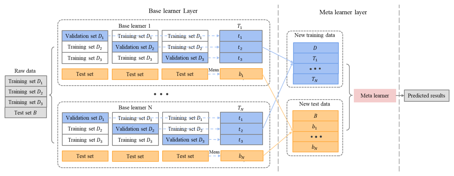
A fundamental requirement of stacking ensemble methods is that the meta-learner must be trained on predictions that the base learners generated for samples they did not observe during their own training. Violating this requirement introduces data leakage: base learners that are first trained on the full training set and subsequently used to predict in-sample observations produce fitted values rather than genuine forecasts, causing the meta-learner to learn a combination rule optimized for interpolation rather than generalization (Wolpert, 1992). To satisfy this requirement, we generate base learner predictions for the meta-learner's training matrix through a K-fold temporal cross-validation scheme. Specifically, the model consists of two layers: the first layer comprises N distinct base learners, while the second layer incorporates a meta-learner. The multi-model fusion prediction workflow of Stacking, based on K-fold cross-validation, can be summarized as follows:

1. Dataset Partitioning. The original dataset is first partitioned into a training set D and a holdout test set B. The training set D is further subdivided into K disjoint subsets, denoted $D_{\mathrm{1}},D_{\mathrm{2}},\mathrm{\dots },D_K$.

2. Base Learner Training. For each base learner $L_n\left(n=\mathrm{1},\mathrm{2},\mathrm{\dots },N\right)$, K-fold cross-validation is performed. In the kth fold, the validation set is D_k and the training set is $D_{(-k)}=D\mathrm{\setminus }{D}_k$. This procedure yields K independently trained instances of each base learner, one per fold.

3. Construction of the Augmented Training Set. Each trained instance of base learner L_n generates out-of-fold predictions on its corresponding validation subset D_k. Concatenating these predictions across all K folds produce a full-length out-of-fold prediction vector T_n for base learner L_n:

   $$\begin{array}{}\text{(14)}& {\mathit{T}}_n=\mathit{\{}{t}_{\mathrm{1}},t_{\mathrm{2}},t_{\mathrm{3}},\mathrm{\dots },t_K\mathit{\}}.\end{array}$$

   The out-of-fold prediction vectors from all N base learners are concatenated with the original training set D to form the augmented training set D^′, which serves as input for the second-level meta-learner:

   $$\begin{array}{}\text{(15)}& D^{\prime }=\mathit{\{}{\mathit{T}}_{\mathrm{1}},{\mathit{T}}_{\mathrm{2}},{\mathit{T}}_{\mathrm{3}},\mathrm{\dots },{\mathit{T}}_N,D\mathit{\}},\end{array}$$

   Upon completion of K-fold cross-validation, each base learner L_n produces K prediction vectors on the holdout test set B, denoted ${\mathit{b}}_n^{\mathrm{1}},{\mathit{b}}_n^{\mathrm{2}},\mathrm{\dots },{\mathit{b}}_n^K$. These K predictions are averaged to yield a single representative test prediction b_n for base learner L_n. The consolidated test predictions from all N base learners are combined with B to form the augmented test set B^′:

   $$\begin{array}{}\text{(16)}& B^{\prime }=\mathit{\{}{\mathit{b}}_{\mathrm{1}},{\mathit{b}}_{\mathrm{2}},{\mathit{b}}_{\mathrm{3}},\mathrm{\dots },{\mathit{b}}_N,B\mathit{\}},\end{array}$$

4. Meta-Learner Training. The augmented dataset D^′ is used to train the second-level meta-learner, and B^′ is used to evaluate its generalisation performance. The meta-learner learns an optimal combination strategy over the base learner outputs, yielding a final ensemble prediction that is expected to surpass any individual constituent model.

The number of folds K is determined by the temporal structure of the data. Since the training dataset spans three complete winter seasons, a 3-fold configuration naturally implements a leave-one-season-out protocol in which each fold corresponds to exactly one complete winter as the validation period. This structure mirrors the real-world forecasting scenario of predicting an unseen winter season from prior observations, and fold boundaries are strictly aligned with seasonal transitions with temporal ordering preserved throughout. The complete workflow is illustrated in Fig. 4.

Figure 4 Architecture of the Stacking Ensemble based on Out-of-Fold Cross-Validation.

2.4 Bayesian ridge regression meta-learner

Since the meta-learner operates on base learner predictions rather than raw input features, its primary role is to learn an optimal fusion of these predictions that accounts for their relative strengths and inter-model correlations. We adopt Bayesian Ridge Regression (BRR; MacKay, 1992) as the meta-learner, motivated by three considerations. First, base learner predictions tend to be correlated due to shared input features; the L2 regularization inherent in BRR effectively alleviates multicollinearity (Hoerl and Kennard, 1970). Second, the Bayesian framework automatically determines the optimal regularization strength through Evidence Maximization, precluding overfitting without manual hyperparameter tuning (Bishop, 2006). Third, BRR yields probabilistic outputs that quantify prediction uncertainty at the ensemble combination layer, conditional on the deterministic base-learner outputs (Gelman and Shalizi, 2013).

The BRR meta-learner assumes a linear relationship between base learner predictions and the observed RST, with Gaussian noise and hierarchical priors on the weight precision:

$$\begin{array}{}\text{(17)}& {\displaystyle }\mathit{y}=\mathbf{X}\mathit{w}+\mathit{ϵ},\mathit{ϵ}\sim \mathcal{N}(\mathrm{0},{\mathit{\alpha }}^{-\mathrm{1}}\mathbf{I}),\text{(18)}& {\displaystyle }\begin{array}{rl}& \mathit{w}\sim \mathcal{N}(\mathrm{0},{\mathit{\lambda }}^{-\mathrm{1}}\mathbf{I}),\mathit{\alpha }\sim \mathrm{Gamma}(a_{\mathrm{0}},b_{\mathrm{0}}),\\ & \mathit{\lambda }\sim \mathrm{Gamma}(c_{\mathrm{0}},d_{\mathrm{0}}),\end{array}\end{array}$$

The posterior distribution over weights is analytically tractable:

$$\begin{array}{}\text{(19)}& \begin{array}{rl}& \mathit{w}\mid \mathit{y},\mathbf{X},\mathit{\alpha },\mathit{\lambda }\sim \mathcal{N}({\mathit{\mu }}_n,{\mathbf{\Sigma }}_n),{\mathbf{\Sigma }}_n=(\mathit{\lambda }\mathbf{I}+\mathit{\alpha }{\mathbf{X}}^{\mathrm{\top }}\mathbf{X}{)}^{-\mathrm{1}},\\ & {\mathit{\mu }}_n=\mathit{\alpha }{\mathbf{\Sigma }}_n{\mathbf{X}}^{\mathrm{\top }}\mathit{y}.\end{array}\end{array}$$

The precision hyperparameters α and λ are optimised via Type-II Maximum Likelihood (Evidence Maximisation), which automatically balances data fit against regularisation without requiring manual cross-validation.

Beyond point prediction, BRR yields a closed-form posterior predictive distribution for each forecast:

$$\begin{array}{}\text{(20)}& p(\stackrel{\mathrm{̃}}{y}\mid x,\mathcal{D})=\mathcal{N}(\stackrel{\mathrm{̃}}{y}\mid {\mathit{\mu }}_n^{\mathrm{\top }}\mathit{x},{\mathit{\sigma }}_n^{\mathrm{2}}(\mathit{x}\left)\right),\end{array}$$

where ${\mathit{\sigma }}_n^{\mathrm{2}}\left(\mathit{x}\right)={\mathit{\alpha }}^{-\mathrm{1}}+x^{\mathrm{\top }}{\mathrm{\Sigma }}_n\mathit{x}$ decomposes total predictive uncertainty into aleatoric noise α⁻¹ and parameter uncertainty encoded in the posterior covariance Σ_n. A separate BRR meta-learner is fitted independently for each forecasting horizon, receiving the two-dimensional out-of-fold prediction vector generated by the two base-learner instances trained for that horizon.

2.5 Multi-Horizon Forecasting Strategy

Multi-step forecasting can be approached through four principal strategies, including recursive, direct, hybrid, and multi-input multi-output (MIMO) approaches (Ben Taieb et al., 2012). In the present study, the direct method is adopted: a fully independent instance of the ensemble is trained separately for each forecasting horizon, with no parameter sharing across horizons. This choice avoids the error accumulation inherent to the recursive and hybrid strategies, and avoids the output-layer distribution mismatch that can arise when a single MIMO model must simultaneously minimise losses at horizons with substantially different error magnitudes. The additional training cost of maintaining three independent model instances is computationally manageable given the offline nature of model development for this application.

3 Experiments

3.1 Datasets and metrics

3.1.1 Site data

This study focuses on a road segment in the northwest inland plain of Jiangsu Province, China, adjacent to the Longhai Railway overpass. The region belongs to a warm temperate semi-humid monsoon climate zone, with minimum daily temperatures in winter reaching approximately −3 °C. The terrain is predominantly flat, which facilitates the horizontal distribution of meteorological variables and minimizes orographic effects that would otherwise compromise the spatial representativeness of gridded reanalysis data.

The primary dataset was collected from road meteorological monitoring station M9393, located west of the Longhai Railway overpass at coordinates (34.30° N, 117.04° E), at a temporal resolution of five minutes. The dataset spans four consecutive winter periods: December 2020 to February 2021, December 2021 to February 2022, December 2022 to February 2023, and December 2023 to February 2024. Infrared remote sensing sensors recorded near-surface meteorological variables including visibility (V), air temperature (AT), relative humidity (RH), precipitation (P), wind speed (WS), wind direction (WD), and road surface temperature (RST), totaling 102 431 raw observations.

Data quality control was applied in several steps. First, the dataset was divided into training and testing subsets. The training subset comprised data from 1 December 2020 to 28 February 2023, and the testing subset comprised data from 1 December 2023 to 29 February 2024. Physically implausible values were then rejected as sensor errors: RST observations exceeding 50 °C or falling below −40 °C, negative precipitation values, and relative humidity outside the range [0 %, 100 %] were removed. For gaps not exceeding one consecutive hour, linear interpolation is applied using the nearest valid observations bracketing the gap, drawn only from that same period. If the right-side interpolation anchor falls within the same natural hour as the missing slot(s), the resulting hourly mean incorporates no observation from any later hour, and no cross-hour information enters the model by construction.

Longer gaps, exceeding one consecutive hour and occurring primarily during scheduled sensor maintenance, were filled using the mean of the observed values recorded at the same hour-of-day and same calendar period across the three training winters, and applied identically regardless of whether the corresponding gap occurred in the training or test period; because this value is derived exclusively from training-period observations at matching calendar times from three prior winters, it introduces no look-ahead information from any test-period observation. This long-gap climatological fill accounts for 1.18 % of 5 min test-period samples at M9393. Following imputation, all variables were resampled to hourly resolution within each period: precipitation was aggregated as the hourly total, and all other variables were computed as hourly means to suppress transient sub-hourly fluctuations. The resulting hourly series exhibits a near-unity variance ratio relative to the native 5 min series and matching significant periodicities (Figs. S1–S2 and Table S1 in the Supplement). This yielded a final dataset of 8664 samples for model development.

RST exhibits significant diurnal periodicity and lag responses to meteorological forcing, reflecting the complex and nonlinear nature of heat exchange at the pavement–atmosphere interface (Cheng et al., 2021). Figure 5 illustrates the daily variation of RST during December 2020, showing a consistent diurnal cycle with a fluctuation range of approximately 5 to 15 °C and strong hour-to-hour autocorrelation across successive days. Figure 6 presents the mean 24 h diurnal RST profile and its 95 % confidence interval computed across the full study period. RST reaches its minimum during the pre-dawn hours, rises gradually through the morning, reaches a mean daily maximum of approximately 6 °C around 14:00, and subsequently declines through the evening. The width of the confidence interval reflects the day-to-day variability at each hour arising from meteorological disturbances superimposed on the underlying diurnal cycle. These characteristics motivate the inclusion of historical RST sequence an input feature.

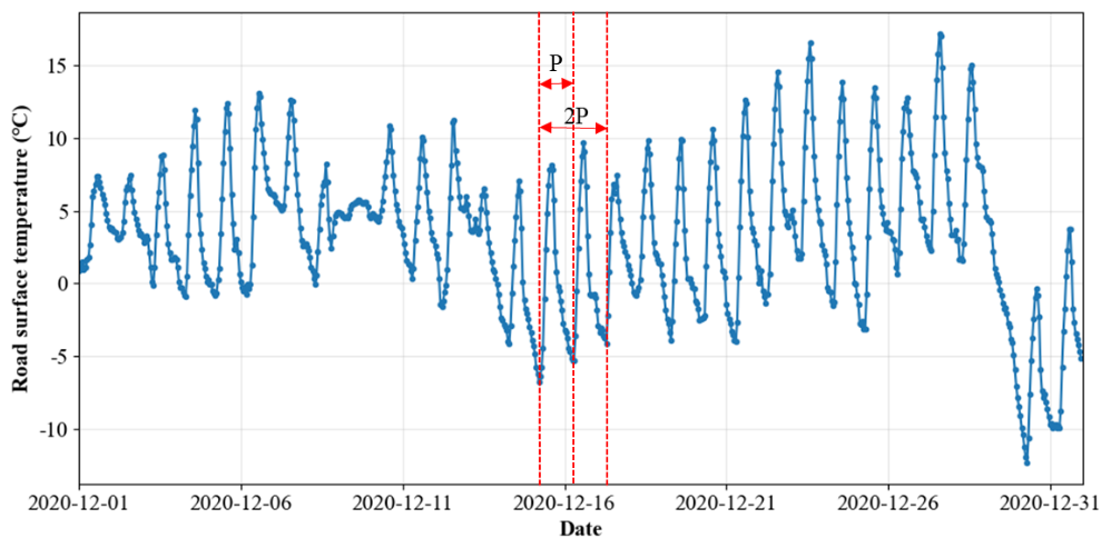
Figure 5 Periodic variation of RST. T represents a period, with time corresponding to one day.

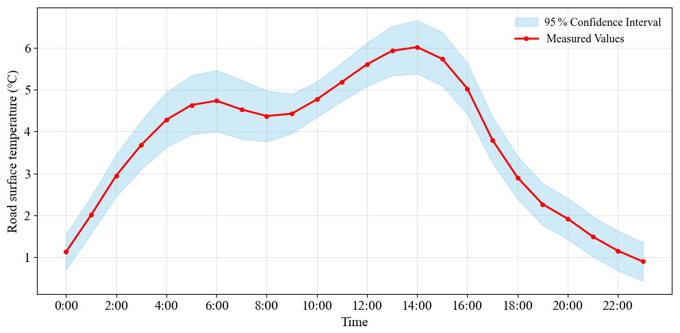
Figure 6 The 24 h diurnal variation curve of RST. The shaded blue part of the graph is the 95 % confidence interval for the RST.

3.1.2 ERA5-Land reanalysis data

ERA5-Land reanalysis data were obtained for the same temporal coverage as the station observations to investigate the potential contribution of physically meaningful auxiliary variables. ERA5-Land is produced by the European Centre for Medium-Range Weather Forecasts (ECMWF) through land surface model simulations driven by ERA5 atmospheric forcing, and is publicly available from the Copernicus Climate Change Service (https://cds.climate.copernicus.eu/, last access: 18 April 2026). The dataset provides hourly estimates at a spatial resolution of 0.1° × 0.1° (approximately 9–11 km), representing area-averaged surface conditions rather than point-scale measurements.

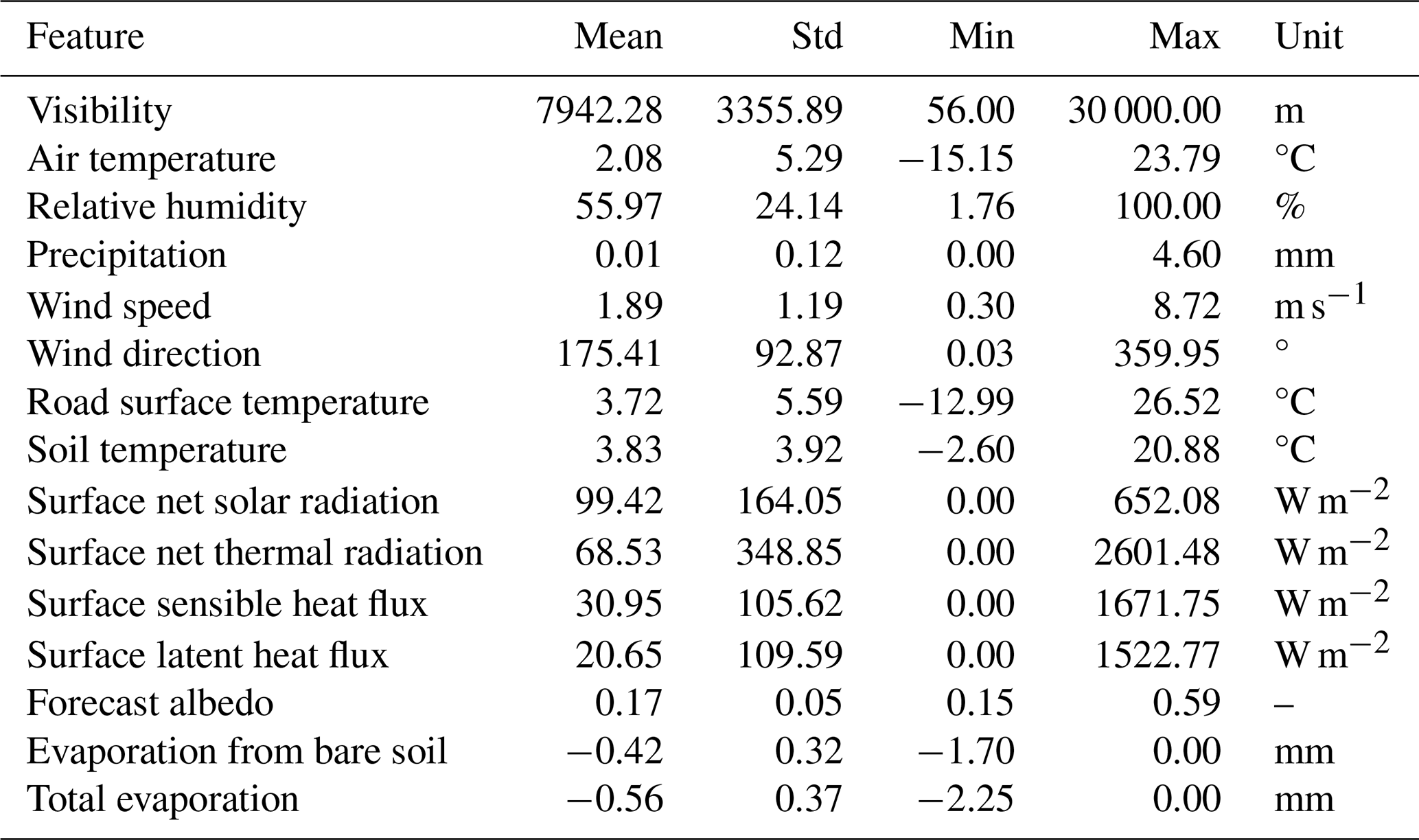
Eight candidate variables with established thermodynamic relevance to road surface temperature dynamics were extracted as the initial variable pool: soil temperature (ST), surface net solar radiation (SSR), surface net thermal radiation (STR), surface sensible heat flux (SSHF), surface latent heat flux (SLHF), forecast albedo (FAL), evaporation from bare soil (EVABS), and total evaporation (E). These variables collectively represent the principal radiative, turbulent, and latent heat exchange terms in the surface energy balance, and their physical relevance to RST evolution is established in the literature (Chen et al., 2019; Hermansson, 2004). Variables ultimately retained for model input were determined through the correlation screening procedure described in Sect. 3.2.

Spatial matching was performed using the nearest-neighbour method, identifying the grid point (34.30° N, 117.00° E) closest to the station. This approach is considered appropriate given the flat terrain of the study region, which minimizes the representativeness error associated with nearest-neighbour interpolation (Muñoz-Sabater et al., 2021). All variables were temporally aligned with the station dataset by converting from UTC to China Standard Time (UTC+8). Unit conversions were applied where necessary: SSR, STR, SSHF, and SLHF, provided as hourly accumulated values in J m⁻², were divided by 3600 to obtain mean flux densities in W m⁻²; ST was converted from Kelvin to degrees Celsius.

Table 2 Summary of the dataset.

3.1.3 Evaluation index

In this study, multiple evaluation metrics are employed to comprehensively evaluate the predictive performance of the models, including the mean absolute error (MAE), root mean squared error (RMSE), symmetric mean absolute percentage error (sMAPE), and coefficient of determination (R²).

$$\begin{array}{}\text{(21)}& {\displaystyle }\mathrm{MAE}={\displaystyle \frac{\mathrm{1}}{n}}{\sum }_{i=\mathrm{1}}^n\left|y_i-{\widehat{y}}_i\right|,\text{(22)}& {\displaystyle }\mathrm{RMSE}=\sqrt{{\displaystyle \frac{\mathrm{1}}{n}}{\sum }_{i=\mathrm{1}}^n(y_i-{\widehat{y}}_i{)}^{\mathrm{2}}},\text{(23)}& {\displaystyle }\mathrm{sMAPE}={\displaystyle \frac{\mathrm{1}}{n}}{\sum }_{i=\mathrm{1}}^n{\displaystyle \frac{\mathrm{2}\left|y_i-{\widehat{y}}_i\right|}{\left|y_i\right|+\left|{\widehat{y}}_i\right|+\mathit{ϵ}}}\times \mathrm{100}\mathit{\%},\text{(24)}& {\displaystyle }{R}^{\mathrm{2}}=\mathrm{1}-{\displaystyle \frac{{\sum }_{i=\mathrm{1}}^n(y_i-{\widehat{y}}_i{)}^{\mathrm{2}}}{{\sum }_{i=\mathrm{1}}^n(y_i-\stackrel{\mathrm{‾}}{y}{)}^{\mathrm{2}}}},\end{array}$$

where y_i is the observed value, ${\widehat{y}}_i$ is the predicted value, $\stackrel{\mathrm{‾}}{y}$ is the mean of the observed values, and n is the total number of samples. and ϵ is a small constant ($\mathit{ϵ}={\mathrm{10}}^{-\mathrm{8}}$) introduced to prevent division by zero when both the observed and predicted values simultaneously approach zero. All reported evaluation metrics were computed exclusively against directly observed RST values; imputed hourly values were retained as model inputs where they occur but were excluded from the evaluation targets.

3.2 Feature extraction

To select a parsimonious and informative input feature set, Spearman rank correlation coefficients (Spearman, 1961) were computed between each candidate variable and winter RST. This nonparametric measure is used in preference to Pearson correlation given the potential for nonlinear monotonic relationships between meteorological variables and RST. The coefficient is calculated as:

$$\begin{array}{}\text{(25)}& \mathit{\rho }=\mathrm{1}-{\displaystyle \frac{\mathrm{6}\mathrm{\Sigma }{\mathrm{d}}_i^{\mathrm{2}}}{n\left(n^{\mathrm{2}}-\mathrm{1}\right)}},\end{array}$$

where d_i is the rank difference between paired observations, and n is the number of samples.

As illustrated in Fig. 7, among the station-observed variables, air temperature exhibits the strongest positive correlation with RST (ρ=0.93), consistent with its recognised role as the primary meteorological driver of near-surface pavement temperature (Chen et al., 2019). Wind speed and precipitation display moderate positive correlations of 0.29 and 0.27, respectively, while relative humidity shows a moderate negative correlation (ρ= −0.25), consistent with the known cooling effect of high-humidity conditions at the pavement surface (Gui et al., 2007). Visibility and wind direction exhibit correlations below 0.20 and are excluded from the input feature set. It is additionally noted that wind direction is a circular variable for which rank-based correlation computed on raw degree values can be misleading; however, the low correlation magnitude observed here is consistent across both conventional and circular-adapted metrics, and the exclusion of wind direction from the final feature set is supported regardless of the association measure applied. The RST sequence is retained as an input variable because, as a directly measured surface quantity, it reflects the integrated effect of prior meteorological forcing at this monitored cross-section and provides information that is complementary to the instantaneous meteorological observations. Based on these findings, the input feature set for the primary analytical perspectives comprises five station-observed variables: AT, RH, P, WS, and historical RST.

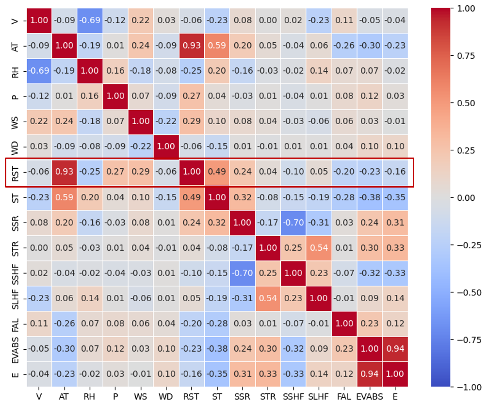
Figure 7 Spearman correlation coefficient plot between RST and various meteorological factors and ERA5_Land physical factors.

For the analytical perspective that investigates the added predictive value of ERA5-Land reanalysis variables (Sect. 4.2, Variable combination 2), the correlation analysis is extended to the full candidate variable pool including both station observations and ERA5-Land fields. Among the ERA5-Land variables, soil temperature shows the strongest positive correlation with RST (ρ=0.49), which may reflect its role as an integrative indicator of subsurface and near-surface thermal conditions. Surface net solar radiation and forecast albedo exhibit correlations of 0.24 and −0.20, respectively, consistent with the known sensitivity of pavement temperature to radiative forcing (Qin et al., 2022). Evaporation from bare soil shows a moderate negative correlation (ρ= −0.23), consistent with the cooling effect associated with surface moisture conditions. The remaining ERA5-Land variables exhibit correlations below 0.20 with RST and are excluded. Accordingly, the augmented input set for Variable combination 2 in Sect. 4.2 comprises nine variables: AT, RH, P, WS, ST, SSR, FAL, EVABS, and historical RST.

3.3 Optimisation

3.3.1 Sliding window size

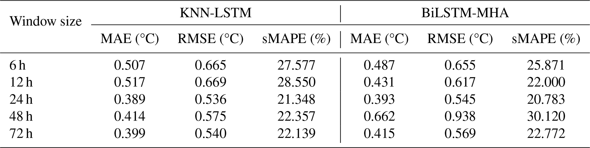
The sliding window method is employed to construct input variables and prediction targets for the model, and the selection of the window size directly influences the ability of the model to capture temperature periodicity and lag effects of meteorological variables. To identify the optimal window size, we conducted a comparative analysis of the improved base models under varying window configurations (Table 3). This analysis revealed that a 24 h sliding window offers an effective balance between predictive performance and computational efficiency, while also matching the timescale of the diurnal RST cycle, enabling the model to learn the recurring day–night thermal rhythm directly from the historical RST and meteorological sequence at this site. Consequently, the 24 h window was selected as the standardized configuration for all subsequent modelling experiments.

Table 3 Impact of sliding window size on errors.

3.3.2 Training

Prior to model training, all variables were standardized using Z-score normalisation to accelerate convergence and eliminate the influence of differing measurement scales. Normalisation parameters were estimated exclusively from the training set to prevent information leakage:

$$\begin{array}{}\text{(26)}& X_{\mathrm{scaled}}={\displaystyle \frac{X_{\mathrm{train}}-{\mathit{\mu }}_{\mathrm{train}}}{{\mathit{\sigma }}_{\mathrm{train}}}},\end{array}$$

where μ_train and σ_train are the mean and standard deviation computed from the training set only. Model outputs were inverse-transformed to degrees Celsius prior to evaluation. Accordingly, all reported MAE and RMSE values are in °C.

To assess the climatological representativeness of the test period, the mean air temperature and RST during the test winter were compared against the three-winter training period mean. The test-period mean air temperature (−1.29 °C) and mean RST (0.49 °C) deviate by less than 1.0 °C from the corresponding training-period means (−0.31 °C and 1.40 °C, respectively), and the proportions of sub-zero RST hours are comparable (45.74 % and 47.53 %). These statistics confirm that the test winter is climatologically representative of the study period and that the evaluation is not materially affected by anomalous thermal conditions.

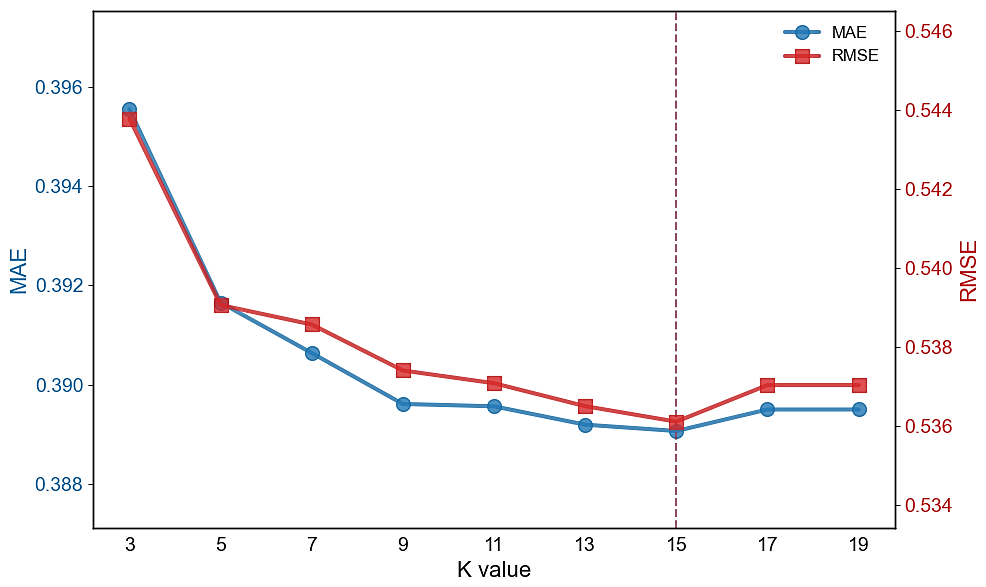
In the KNN-LSTM model, the hyperparameter K specifies the number of nearest-neighbour historical sequences used to construct the similarity feature matrix F_t, and directly governs the trade-off between local pattern specificity and representational stability. A value of K that is too small risks overfitting to unrepresentative neighbours, while an excessively large K may dilute the local similarity signal by averaging over dissimilar historical states. To determine the optimal K, a grid search over $K\in \mathit{\{}\mathrm{3},\mathrm{5},\mathrm{7},\mathrm{9},\mathrm{11},\mathrm{13},\mathrm{15},\mathrm{17},\mathrm{19}\mathit{\}}$ was conducted by evaluating MAE and RMSE on the validation set. As shown in Fig. 8, both metrics decrease monotonically with increasing K, reaching their minimum at K=15, beyond which performance stabilizes. Accordingly, K=15 is adopted as the fixed hyperparameter for all subsequent experiments. It should be noted that this search is a one-time offline procedure performed during model development; during inference, the KNN-LSTM model executes a single forward pass using the fixed K=15, incurring no additional computational overhead.

Figure 8 The effect of K value on MAE and RMSE.

The KNN-LSTM model employs a three-layer LSTM architecture with 64, 32, and 16 hidden units in successive layers, with tanh activation in the first layer and ReLU in deeper layers to mitigate the vanishing gradient problem (Glorot et al., 2011). The BiLSTM-MHA model uses a bidirectional LSTM with 128 units per direction, followed by a multi-head attention mechanism with 4 heads and key dimension 64, layer normalisation with residual connection, global average pooling, and a single-unit dense output layer. Both models are trained with the Adam optimizer (Kingma and Ba, 2014) at a learning rate of 0.001, mean squared error loss, batch size 32, a maximum of 100 epochs, and early stopping with patience 20 to prevent overfitting. L2 regularization is applied to all LSTM layers to further improve generalization. This architecture and training configuration is shared across the three forecasting horizons; for each horizon, a separate model instance with this identical configuration is trained independently, yielding horizon-specific weights with no parameter sharing across horizons.

3.4 Complementarity and ablation analysis

The effectiveness of a stacking ensemble depends critically on base learner diversity: models that commit errors in different input regions enable the meta-learner to achieve superior performance beyond any individual component. Computational constraints limit the number of base learners, as each requires independent out-of-fold training across all folds. KNN-LSTM and BiLSTM-MHA are selected for their partially complementary predictive characteristics with respect to winter RST spatiotemporal structure. KNN-LSTM integrates similarity-based feature augmentation with sequential modelling to identify local pattern recurrence through retrieval of analogous historical meteorological states, making it effective at capturing regime-specific behaviours tied to locally recurring weather conditions. BiLSTM-MHA employs bidirectional recurrent processing with multi-head self-attention to dynamically weight temporal features across the full input window, demonstrating superior capability in extracting global temporal dependencies and long-range patterns during thermally complex periods involving sustained trends or abrupt transitions.

To empirically validate this complementarity prior to ensemble construction, we conduct a complementarity analysis and an ablation study, both at the 1 h forecasting horizon where the ensemble signal is cleanest. Results are presented in Fig. 9 and Table 4. The Pearson correlation coefficient between the residual series of the two base learners is r=0.889, indicating substantial but imperfect co-variation in prediction errors. However, a high global correlation does not preclude conditional complementarity across distinct operating regimes (Kuncheva and Whitaker, 2003). As shown in Fig. 9b, the two models exhibit asymmetric error patterns across temperature regimes: under sub-zero conditions, BiLSTM-MHA achieves a lower MAE, whereas under above-zero conditions KNN-LSTM is more accurate. This regime-dependent asymmetry is noteworthy because sub-zero and above-zero conditions are typically associated with distinct meteorological forcing characteristics – sustained radiative cooling under clear skies versus more variable radiation-driven heating, respectively (Hermansson, 2004; Qin et al., 2022) – suggesting that the two architectures may be exploiting different statistical regularities in the RST signal. Figure 9c shows comparable daytime and nighttime performance at the aggregate level, indicating that temperature-regime complementarity, rather than the diurnal cycle per se, is the dominant source of predictive diversity between the two base learners. Figure 9d further confirms that neither model achieves consistent sample-level dominance, demonstrating sustained bidirectional predictive diversity that the meta-learner can systematically exploit.

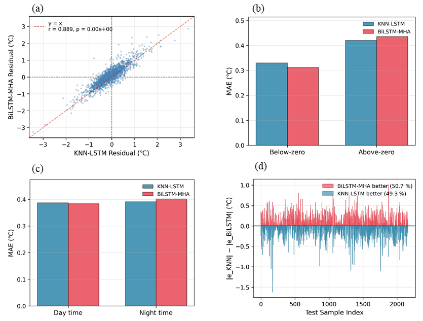
Figure 9 Complementarity analysis of base learners: (a) residual correlation analysis, (b) temperature interval error decomposition, (c) day and night time error decomposition, and (d) time series advantage distribution.

Three ablation configurations are evaluated to quantify the independent contribution of each architectural innovation (Table 4). Config-1 (LSTM + BiLSTM) establishes the baseline ensemble without any proposed innovations; Config-2 (LSTM + BiLSTM-MHA) isolates the contribution of multi-head attention by introducing the MHA mechanism to the second base learner while retaining the standard LSTM as the first; Config-3 (KNN-LSTM + BiLSTM) isolates the contribution of KNN-based similarity augmentation by replacing the first base learner with KNN-LSTM while retaining the standard BiLSTM as the second; and the full ILES (KNN-LSTM + BiLSTM-MHA) achieves the best performance across all metrics. Relative to Config-1, introducing multi-head attention alone reduces MAE by 0.035 °C (8.20 %), whereas introducing KNN-based similarity augmentation alone reduces MAE by 0.044 °C (10.30 %). Yet the combined gain of ILES (0.054 °C) is smaller than the arithmetic sum of the two individual gains (0.079 °C), indicating that KNN-LSTM and BiLSTM-MHA partially share their areas of improvement; nonetheless, the full ILES framework achieves the best overall performance, confirming that the two components provide partially complementary rather than redundant or synergistic contributions.

Table 4 Ablation study on the effect of multi-head attention and KNN-based similarity augmentation.

3.5 Prediction performance evaluation

To systematically evaluate the proposed ILES framework and address the four objectives stated in Sect. 1, four analytical perspectives are designed as follows.

1. Comprehensive performance benchmarking. ILES is evaluated against ten models spanning three categories: a naive persistence baseline, nonlinear regression, traditional machine learning methods (Random Forest, XGBoost), standard deep learning architectures (GRU, LSTM, BiLSTM, CNN-LSTM), and the two proposed base learners (KNN-LSTM, BiLSTM-MHA). All models receive identical station-only inputs and are evaluated at 1, 3, and 6 h forecasting horizons using MAE, RMSE, sMAPE, and R².

2. Input configuration comparison. Three input variable combinations are evaluated at the 1, 3, and 6 h forecasting horizons to assess the relative predictive value of different information sources. Variable combination 1 comprises the five directly observed meteorological variables: AT, RH, P, WS, and lagged RST. Variable combination 2 extends Variable combination 1 with four ERA5-Land reanalysis variables – ST, SSR, FAL, and EVABS – selected on the basis of Spearman rank correlation with winter RST. Variable combination 3 extends Variable combination 1 with four derived features constructed exclusively from existing station observations T_grad, and RST temporal tendency features at 1, 3, and 6 h lags (ΔRST_1 h, ΔRST_3 h, ΔRST_6 h).

3. Feature importance and model interpretability. SHAP analysis is applied to ILES under the station-only configuration to quantify the marginal contribution of each input feature to individual predictions. Attribution values are examined stratified by temperature regime and across the diurnal cycle. The resulting feature importance patterns are qualitatively compared with expectations derived from established meteorological understanding of near-surface heat exchange processes, serving as a plausibility check on the model's learned input–output behaviour.

4. Multi-site validation. The cross-site applicability of the ILES framework is assessed at two independent stations, M9474 and M9448, using station-only inputs at the 1 h horizon. At each station, the framework is retrained independently on site-specific observations following the same protocol as the primary site. Performance rankings across five deep learning models are compared at all three stations to determine whether the predictive advantages of the ensemble are site-specific or structurally consistent across different road environments within the temperate monsoon climate zone. Uncertainty quantification provided by the BRR meta-learner is additionally assessed through a reliability diagram on the held-out test set.

4 Results

4.1 Multi-horizon prediction performance

Table 5 presents the prediction performance of eleven models across 1, 3, and 6 h forecasting horizons. The model hierarchy spans a naive persistence forecasting (assuming RST at time t+h equals RST at time t), a nonlinear regression baseline (NR), traditional machine learning methods (RF, Darghiasi et al., 2025; XGBoost, Kebede et al., 2024), standard deep learning architectures (GRU, LSTM, BiLSTM, CNN-LSTM, Tabrizi et al., 2021), the two proposed base learners (KNN-LSTM, BiLSTM-MHA), and the proposed ensemble ILES.

Table 5 Performance evaluation across 1, 3, and 6 h forecasting intervals. The last three models (KNN-LSTM, BiLSTM-MHA, ILES) represent the novel architectures proposed in this study. The preceding eight models serve as representative baselines from established model families. All models are trained and evaluated on the same dataset under the same protocol. Pairwise significance testing supporting the performance rankings reported in this table is provided in Tables S2 and S3.

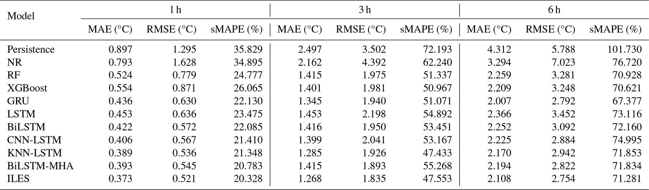
At the 1 h horizon, persistence yields an MAE of 0.897 °C, RMSE of 1.295 °C, and sMAPE of 35.829 %, establishing a lower bound of predictive skill that any learned model should substantially exceed. ILES reduces MAE by 58.42 % relative to persistence and by 52.96 % relative to NR, indicating that the learned temporal representations capture substantially more information than either the most recent observation or a simple parametric reference model. Relative to the traditional machine learning baselines, RF and XGBoost, ILES reduces MAE by 28.82 % and 32.67 % respectively. Relative to the four standard deep learning architectures, GRU, LSTM, BiLSTM, and CNN-LSTM, ILES reduces MAE by 8.13 % to 17.66 %, with the smallest margin against CNN-LSTM, the strongest of the four. Relative to its own base learners, ILES reduces MAE by 4.11 % over KNN-LSTM and 5.09 % over BiLSTM-MHA.

At the 3 h horizon, the performance gap between persistence and all learned models widens further, consistent with the increasing value of temporal modelling at longer lead times. ILES reduces MAE by 49.22 % relative to persistence and 41.35 % relative to NR. Against the traditional machine learning and standard deep learning baselines collectively, RF, XGBoost, GRU, LSTM, BiLSTM, and CNN-LSTM, ILES reduces MAE by 5.72 % to 12.73 %. Relative to its own base learners, the margin narrows to 1.32 % over KNN-LSTM, the strongest individual model at this horizon, and 10.39 % over BiLSTM-MHA.

At the 6 h horizon, persistence skill degrades substantially, underscoring the practical necessity of learned models at extended lead times. ILES reduces MAE by 51.11 % relative to persistence and 36.00 % relative to NR. Among the six traditional machine learning and deep learning baselines, ILES achieves lower MAE than five, with reductions ranging from 4.57 % to 10.90 %, while GRU attains a marginally lower MAE than ILES by 5.03 %. ILES nonetheless maintains the lowest RMSE among all eleven models at this horizon. Relative to its own base learners, ILES reduces MAE by 2.86 % over KNN-LSTM and 3.92 % over BiLSTM-MHA. sMAPE values increase substantially across all models at this horizon, reflecting the prevalence of near-zero RST values in winter conditions, which inflates this metric independent of absolute forecast accuracy; MAE and RMSE remain the more informative indicators at extended horizons.

Across all three horizons, ILES achieves the lowest MAE and RMSE among the eleven evaluated models, with the single exception of GRU's marginally lower MAE at 6 h. sMAPE rankings are less consistent: KNN-LSTM attains a marginally lower sMAPE at 3 h, and GRU, XGBoost, and RF attain lower sMAPE at 6 h. The magnitude of improvement varies predictably with baseline category and forecasting horizon: gains over persistence and NR remain large at every horizon, ranging from 36 % to 58 %, while gains over the established machine learning and deep learning baselines narrow from roughly 8 %–33 % at 1 h to 5 %–13 % at 3 h and 5 %–11 % at 6 h, and the margin over the two base learners is smaller still, between 1 % and 10 % across horizons. This gradient is consistent with a model that captures genuine temporal structure beyond what persistence or simple regression can represent, while offering a more modest but directionally consistent refinement over architecturally related deep learning baselines and its own constituent base learners.

Figure 10 presents density scatter plots of predicted versus observed RST for five models across three forecasting horizons, enabling both cross-horizon and cross-model comparison of goodness-of-fit and error structure.

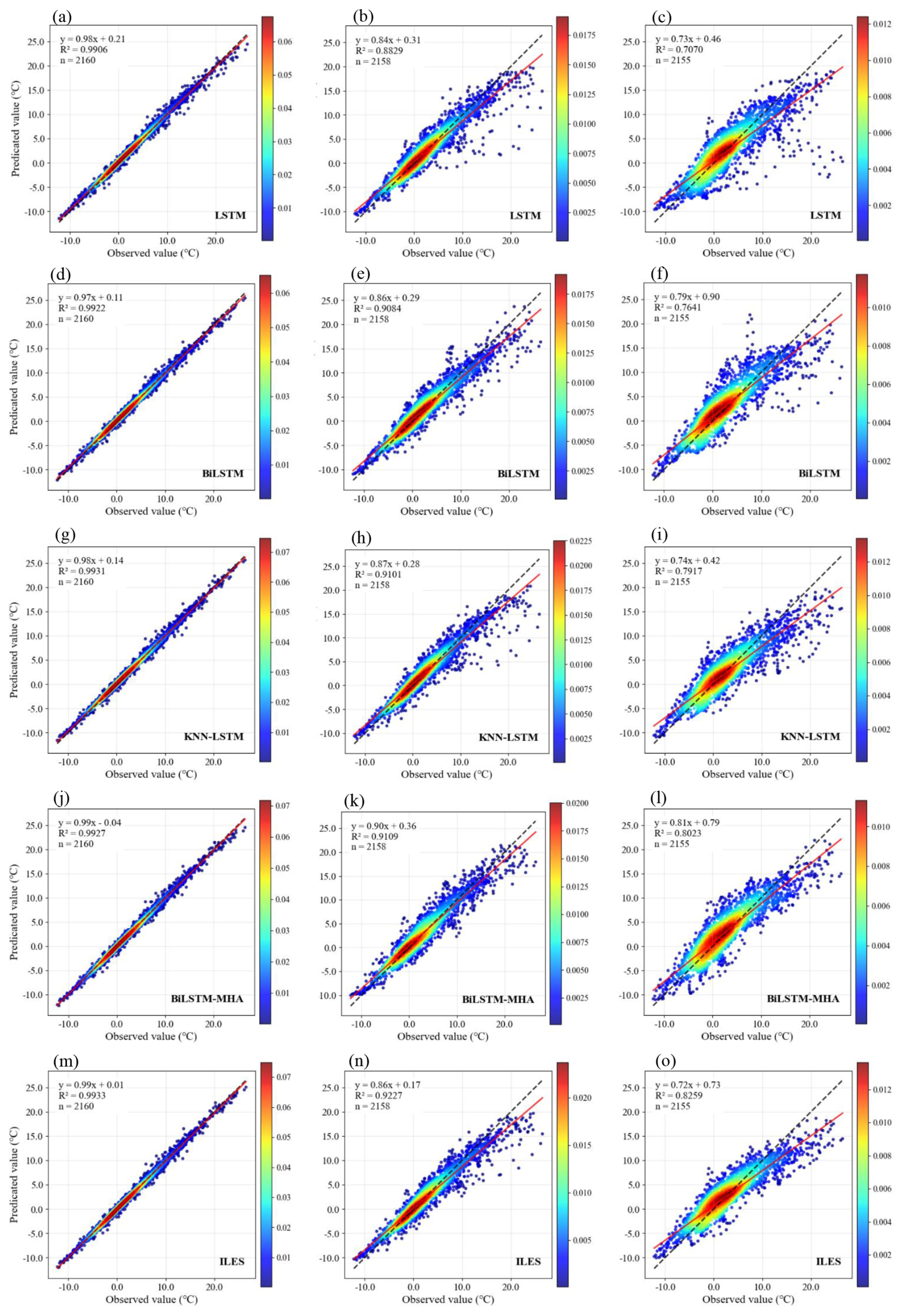
Figure 10 Density scatter plots of predicted versus observed winter RST across 1 h (a, d, g, j, m), 3 h (b, e, h, k, n), and 6 h (c, f, i, l, o) forecasting intervals. Here, colours indicate the kernel density estimation (KDE) of point concentration, with red representing high-density regions and blue representing low-density regions. Colour bar scales differ across panels to optimize the visualization of density distribution within each forecasting horizon.

Across all models, predictive accuracy degrades systematically with forecast lead time. At the 1 h horizon, scatter points cluster tightly along the y=x line with high-density regions concentrated near the origin, reflecting strong model fit. At 3 and 6 h, progressive dispersion is observed: high-density regions contract, outliers increase in frequency, and regression slopes deviate increasingly from unity, indicating that all models struggle to capture rapid thermal transitions at extended horizons.

Across models at the 1 h horizon, LSTM achieves R²=0.9906 with a regression slope of 0.98, while BiLSTM, KNN-LSTM, and BiLSTM-MHA show progressive improvement consistent with their architectural advances. ILES attains the highest goodness-of-fit, with scatter points most tightly concentrated along the ideal line. At the 3 h horizon, the performance hierarchy is preserved: ILES achieves R²=0.9227, outperforming LSTM, BiLSTM, KNN-LSTM, and BiLSTM-MHA. At the 6 h horizon, ILES maintains R²=0.8259, compared to 0.7070 for LSTM, whose scatter plot exhibits the broadest dispersion and most prominent systematic underestimation at high RST values.

A consistent pattern across all models and horizons is that prediction errors increase with RST magnitude, as evidenced by the progressive transition from high- to low-density regions at elevated temperatures. This effect is most pronounced at the 6 h horizon, where outlier frequency increases sharply above 10 °C across all architectures, likely reflecting the greater complexity and variability of RST dynamics under daytime heating conditions, which are not directly represented in the model inputs (Qin et al., 2022). Notably, ILES exhibits the most restrained error growth with temperature, suggesting that ensemble integration partially compensates for this systematic limitation.

4.2 Input variable combinations comparison

Three input configurations are evaluated to investigate the relative predictive value of different information sources and to determine whether domain-knowledge-guided feature construction provides a practically deployable alternative to reanalysis augmentation for operational RST forecasting.

1. Variable combination 1 comprises AT, RH, P, WS, and historical RST, corresponding to the standard observational feature set adopted in Sect. 4.1 and serving as the reference configuration.

2. Variable combination 2 supplements Variable combination 1 with ERA5-Land-derived variables, including ST, SSR, FAL, and EVABS, representing an attempt to recover physically meaningful forcing information through grid-scale reanalysis surrogates.

3. Variable combination 3 supplements Variable combination 1 with four physically motivated features derived directly from existing station observations. The surface–air temperature difference, defined as $T_{\mathrm{grad}}=T_{\mathrm{RST}}-T_{\mathrm{AT}}$, encodes the sign and magnitude of the near-surface thermal contrast at the pavement–atmosphere interface. This quantity serves as a first-order indicator of the direction of turbulent sensible heat exchange: positive values correspond to daytime conditions under which the road surface is warmer than the overlying air, while negative values are characteristic of nocturnal radiative cooling and are commonly associated with elevated icing risk (Hermansson, 2004). The RST temporal tendency features ΔRST_τ for $\mathit{\tau }\in \left\{\mathrm{1},\mathrm{3},\mathrm{6}\right\}$ hours quantify the rate of change of road surface temperature over multiple time scales, providing explicit multi-scale descriptors of pavement thermal dynamics alongside the absolute RST sequence. T_grad provides a direct, station-measured indicator of the surface–air thermal contrast, and ΔRST_τ provides an empirical, multi-scale descriptor of the rate of RST change; both are physically motivated by the surface energy balance framework introduced in Sect. 1, without requiring additional sensor infrastructure. Each feature combination is subsequently used as the input feature matrix X fed into the ILES model.

Performance under sub-zero conditions is assessed on the longest continuous segment of test samples satisfying RST < 0 °C, spanning from 16:00 on 19 February 2024 to 03:00 on 22 February 2024 and comprising 60 consecutive hourly samples. This segment-based evaluation is adopted to provide a coherent assessment of model behaviour during a sustained cooling event, which constitutes the most operationally critical scenario for road icing risk assessment (Song et al., 2023; CMA, 2018).

As shown in Table 6, Variable combination 3 achieves the lowest MAE and RMSE across all three forecasting horizons. Its sMAPE is also lowest at the 1 and 3 h horizons. At the 1 h horizon, it attains an MAE of 0.19 °C and RMSE of 0.23 °C, representing reductions of 28.70 % and 30.10 % relative to Variable combination 1, and 42.60 % and 45.10 % relative to Variable combination 2. At 3 h, Variable combination 3 reduces MAE by 43.50 % and RMSE by 45.50 % relative to Variable combination 1, and by 48.00 % and 41.20 % relative to Variable combination 2. At 6 h, Variable combination 3 continues to yield the lowest MAE and RMSE, while Variable combination 2 remains the weakest performer across all metrics and horizons.

Table 6 Prediction performance of the ILES model with three input variable combinations in the subzero low temperature period.

Figure 11 corroborates this hierarchy visually. At the 1 h horizon, Variable combination 3 tracks the observed cooling descent from 20 to 21 February most faithfully, while combinations 1 and 2 exhibit systematic underestimation of the cooling rate. This behaviour is consistent with the role of T_grad and ΔRST_τ in supplying explicit thermal contrast and rate-of-change information during periods of sustained temperature decline, when these signals are most informative. At 3 and 6 h horizons, all configurations show progressive amplitude attenuation; Variable combination 2 exhibits the most pronounced phase lag and amplitude underestimation, while Variable combination 3 retains the closest agreement with observed thermal minima.

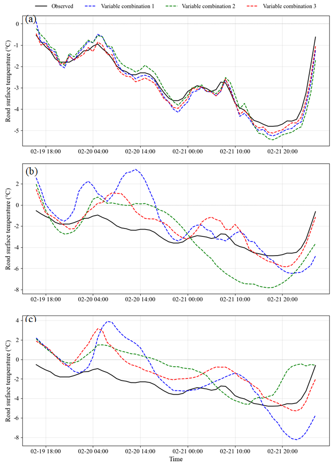
Figure 11 Winter RST prediction of ILES model with three input variable combinations in subzero low temperature period across 1 h (a), 3 h (b), and 6 h (c) forecasting intervals. This period is the longest continuous section of the test sample with RST < 0  °C.

The degraded performance of Variable combination 2 is attributable to two mechanisms. First, ERA5-Land provides area-averaged estimates at approximately 9 to 11 km resolution, whereas RST is governed by point-scale surface conditions; this spatial representativeness mismatch introduces estimation errors that reduce rather than enhance predictive content, a well-documented limitation of gridded reanalysis products in surface applications (Muñoz-Sabater et al., 2021). Second, the historical RST sequence included in all three configurations already implicitly encodes the net effect of prior meteorological forcing at the pavement surface, rendering the reanalysis-derived surrogates largely redundant while simultaneously increasing input dimensionality (Reichstein et al., 2019). These conclusions are specific to the instrumented, data-rich setting examined here; in station-sparse regions, reanalysis variables may retain supplementary predictive value provided that appropriate bias correction is applied to mitigate the identified scale mismatch.

To assess whether the performance hierarchy established under sub-zero conditions reflects a general advantage of Variable combination 3 rather than a regime-specific result, two three-day periods are further examined: a stable clear-sky period (25 to 27 January 2024, characterised by mean relative humidity below 50 %, zero precipitation, and wind speeds below 2 m s⁻¹) and an overcast rainy period (23 to 25 February 2024, characterised by continuous precipitation and relative humidity exceeding 85 %). These two periods represent contrasting RST variability regimes, spanning periodically dominated and stochastically driven conditions, with direct relevance to operational winter road maintenance (Darghiasi et al., 2023).

Under overcast and rainy conditions (Fig. 12a to c), RST variability becomes markedly more subdued and irregular. Variable combination 2 exhibits the most severe performance degradation across all horizons, with persistent positive bias and substantial loss of observed thermal structure at 6 h, attributable to the introduction of spatially mismatched reanalysis information under precipitation-dominated conditions. Variable combination 3 consistently maintains the closest correspondence with observations, with its relative advantage most pronounced at 3 and 6 h.

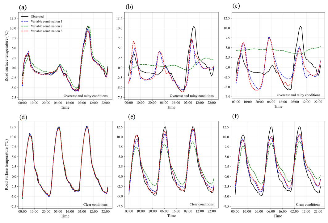
Figure 12 Winter RST prediction of ILES model with three input variables in overcast and rainy and clear synoptic conditions across 1 h (a, d), 3 h (b, e), and 6 h (c, f) forecasting intervals.

Under clear-sky conditions (Fig. 12d to f), RST exhibits pronounced diurnal oscillations with peak-to-trough amplitudes of approximately 17 °C. At the 1 h horizon, all three configurations achieve comparable accuracy. At 3 and 6 h, Variable combination 2 shows progressive amplitude underestimation, while Variable combination 3 maintains the closest alignment with the observed diurnal cycle, consistent with the high predictive content of multi-scale tendency features under regular periodic forcing.

Taken together, the results across sub-zero, clear-sky, and overcast regimes consistently favour Variable combination 3, confirming that physics-motivated feature engineering provides the most effective input strategy for station-based winter RST prediction at instrumented sites. Accordingly, Variable combination 1 is retained as the standard input configuration for Sect. 4.3 and 4.4. Since all ten benchmark models in Sect. 4.1 were evaluated under this configuration, retaining it as the reference ensures that SHAP-based attribution and cross-site performance rankings remain directly comparable to the established benchmarks without confounding from input differences. It should be noted that in operational settings where physics-motivated feature construction is feasible, variable combination 3 is recommended as the preferred input strategy given its consistently lowest MAE and RMSE across all forecasting horizons and meteorological regimes.

4.3 Feature importance and model interpretability

To examine the degree to which the learned input–output relationships of the ILES model are consistent with established meteorological understanding of RST dynamics, SHAP analysis is applied under the station-only input configuration (Variable combination 1). Since the BRR meta-learner operates on base learner predictions rather than raw meteorological features, SHAP values cannot be applied directly to the ensemble output to attribute importance to the original inputs. Instead, KernelSHAP (Lundberg and Lee, 2017) is applied independently to each base learner (KNN-LSTM and BiLSTM-MHA) with respect to the original input feature set, treating each base learner as a black-box function mapping raw features to RST predictions. The resulting SHAP values from the two base learners are aggregated as a weighted average, with weights proportional to the BRR meta-learner coefficients, to produce a single set of feature attributions representative of the full ensemble. This procedure provides a model-agnostic and theoretically principled attribution of ensemble predictions to the original meteorological inputs, grounded in cooperative game theory (Lundberg and Lee, 2017; Joo et al., 2023). Attribution values are examined stratified by temperature regime and across the diurnal cycle, enabling a systematic assessment of whether the learned importance structure is qualitatively consistent with the dominant meteorological drivers identified by surface energy balance theory.

The SHAP analysis presented here is restricted to the four instantaneous meteorological input variables (AT, RH, WS, P). The reported SHAP importances therefore characterise the marginal contributions of the contemporaneous meteorological state, not the full input space. AT is the dominant predictor (Fig. 13a), with a mean absolute SHAP value of 0.696, accounting for 55.4 % of total feature importance. RH, WS, and P follow in descending order, contributing 16.9 %, 14.3 %, and 13.4 % respectively. This ranking is consistent with the recognized role of AT as the primary driver of RST through near-surface sensible heat exchange, and the secondary modulating roles of RH, WS, and P through evaporative, convective, and latent heat processes (Chen et al., 2019; Gui et al., 2007; Feng and Feng, 2012). The beeswarm plot (Fig. 13b) confirms the expected directionality: high AT values are associated with positive SHAP contributions across the full temperature range, while elevated RH and P values are predominantly associated with negative contributions, consistent with their cooling influence under high-humidity and wet-surface conditions. The narrow spread of P points reflects its episodic character, with predictive influence concentrated in a small fraction of precipitation hours.

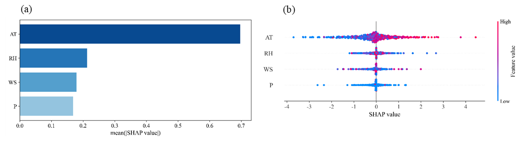
Figure 13 Mean absolute SHAP values (a) and beeswarm plots of SHAP value distributions (b) for the ILES model.

Figure 14a presents the diurnal evolution of mean absolute SHAP values. AT maintains the highest importance at all hours, with moderately elevated values during the solar heating window (09:00 to 16:00) and the nocturnal cooling window (22:00 to 06:00), broadly consistent with the larger surface-air thermal contrast expected during these periods. RH, WS, and P display comparatively stable diurnal profiles without systematic hour-to-hour variation. Figure 14b presents importance values stratified by RST regime. AT importance is notably elevated at thermal extremes, with mean absolute SHAP values of 1.603 at RST below −5 °C and 1.380 at RST above 15 °C, compared to 0.224 in the 0 to 5 °C range, consistent with the larger surface-air temperature differences expected under extreme thermal conditions. In the near-neutral regime (0 to 5 °C), feature importances are compressed across all variables, indicating reduced dominance of any single predictor. In the above-15 °C regime, P rises to second rank with a mean absolute SHAP value of 0.419, though the small sample size in this stratum (n=56) warrants caution in interpretation.

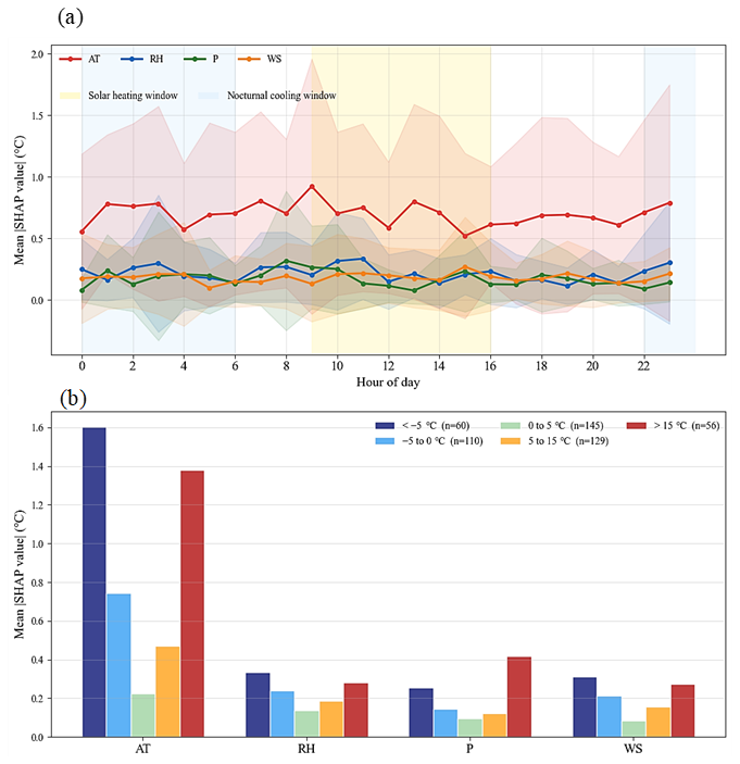
Figure 14 Diurnal variation of mean absolute SHAP values across the 24 h cycle (a). Shaded regions indicate the solar heating window (09:00–16:00) and nocturnal cooling window (22:00–06:00). Mean absolute SHAP values stratified by RST regime (b). Numbers in parentheses indicate sample counts per regime.

Collectively, the SHAP results indicate that the ILES model has learned importance rankings that are qualitatively consistent with the primary meteorological drivers of RST identified by surface energy balance theory, across both precipitation states and temperature regimes. It should be noted that SHAP analysis characterises learned statistical associations and does not establish causal correspondence with physical processes; the consistency identified here is a necessary but not sufficient condition for physical plausibility.

4.4 Multi-site validation

To assess the cross-site applicability of the proposed ILES framework, validation was conducted at two independent stations: M9474 (Xiaohuangshan, 32.04° N, 119.86° E) and M9448 (Huai'an Airport, 33.75° N, 119.17° E), both located on the central Jiangsu plain. M9474 is situated on a cross-Yangtze River bridge, approximately 363 km southeast of the primary station; M9448 is located near Huai'an Airport, approximately 206 km southeast of M9393, on flat open terrain. As with the primary station M9393, both M9474 and M9448 are situated in relatively unobstructed settings without significant roadside screening structures; this validation therefore assesses transferability of the framework's architecture and training protocol across stations sharing broadly similar exposure geometries, rather than across the specific shading or sky-view conditions encountered at screened road segments. The input variables at both stations comprise site-specific air temperature, wind speed, relative humidity, precipitation, and historical RST. Consistent with the imputation procedure described in Sect. 3.1.1, no short-gap event in the test period has a cross-hour interpolation anchor at either validation station, and long-gap climatological fills – computed using the same station-specific, training-period-only procedure – account for 0.66 % and 0.13 % of 5 min test-period samples at M9474 and M9448, respectively. For M9474, the winter of 2024 served as the test set. For M9448, three winter seasons (January–February 2017, December 2017–February 2018, and December 2018–February 2019) were used for training, with December 2019–February 2020 as the test set. At each site, the ILES framework was retrained independently on site-specific observations following the same experimental protocol as described in Sect. 3.3.2.

Table 7 presents the 1 h prediction results at all three stations. ILES consistently outperforms the standard LSTM model at all three sites, with MAE reductions of 17.66 %, 5.68 %, and 35.65 % at M9393, M9474, and M9448, respectively. The consistent performance advantage of ILES across stations with distinct surface conditions confirms the structural robustness of the proposed approach within the temperate monsoon climate zone.

Table 7 Comparison of MAE, RMSE, and sMAPE for 1 h winter RST prediction at M9393, M9474 and M9448 sites using five deep learning models.

The BRR meta-learner yields closed-form probabilistic forecasts through its posterior predictive distribution (Eq. 20). Figure 15 presents reliability diagrams evaluated on the held-out test sets at all three stations, in which the empirical coverage curves lie consistently above the diagonal of perfect calibration across all nominal confidence levels, indicating systematic conservative over-coverage at each site. At M9393, the 68 %, 90 %, and 95 % prediction intervals achieve empirical coverages of 88.1 %, 96.8 %, and 98.1 %, with mean interval widths of 1.523, 2.519, and 3.000 °C, respectively. At M9474, the corresponding coverages are 88.1 %, 95.6 %, and 97.5 %, with mean widths of 0.967, 1.600, and 1.906 °C. At M9448, coverages of 88.1 %, 95.6 %, and 97.5 % are achieved with mean widths of 2.216, 3.666, and 4.368 °C. The notably narrower intervals at M9474 relative to M9393 reflect the lower RST variability characteristic of the bridge-mounted station, while the consistent coverage hierarchy across all three sites confirms that the conservative calibration pattern is a structural property of the BRR posterior predictive decomposition (Eq. 20) rather than a site-specific artefact.

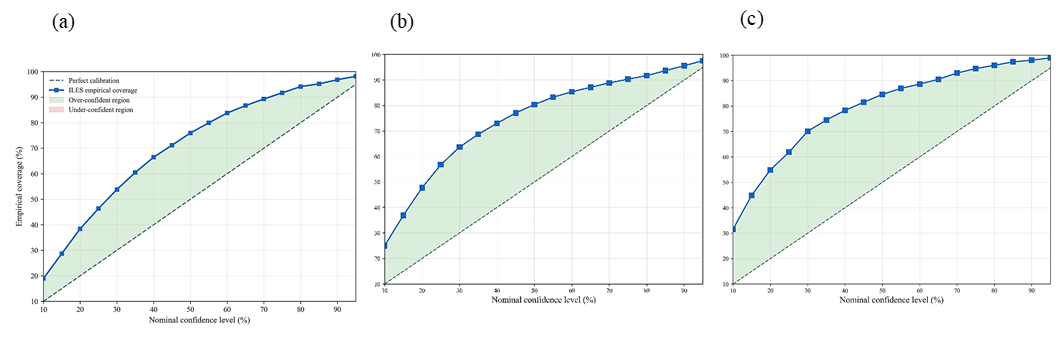
Figure 15 Reliability diagrams of the BRR meta-learner for 1 h winter RST prediction at M9393, M9474, and M9448.

5 Conclusion

This study proposed the Improved LSTMs Ensemble with Stacking (ILES) framework for winter road surface temperature prediction, integrating two base learners with partially complementary predictive characteristics within a stacking ensemble trained via three-fold temporal cross-validation aligned to complete winter seasons. The framework was evaluated across four analytical perspectives using four consecutive winters of observations from an operational road meteorological station in Jiangsu, China.

On predictive performance, ILES generally achieved the lowest prediction errors among all eleven evaluated models at each of the 1, 3, and 6 h forecasting horizons, with MAE ranging from 0.373 °C at 1 h to 2.108 °C at 6 h and R² reaching 0.993, 0.923, and 0.826, respectively. Against the six established machine learning and deep learning baselines – RF, XGBoost, GRU, LSTM, BiLSTM, and CNN-LSTM – ILES reduced MAE by 8.13 %–32.67 % and RMSE by 8.11 %–40.18 % at 1 h, and cut MAE by 5.72 %–12.73 % and RMSE by 5.41 %–16.51 % at 3 h; at 6 h, ILES achieved lower MAE and RMSE than five of the six established baselines, the exception being GRU, though ILES retained the lowest RMSE across all eleven models. sMAPE rankings were not uniformly optimal: at the 6 h horizon, GRU, XGBoost, and RF achieved lower sMAPE than ILES, a pattern attributable to the disproportionate sensitivity of sMAPE to near-zero RST values at extended horizons.

On input configuration, physics-motivated feature engineering incorporating the surface–air temperature difference and multi-scale RST temporal tendency features achieved the lowest MAE and RMSE relative to both the station-only observational baseline and ERA5-Land reanalysis augmentation across all forecasting horizons and meteorological regimes examined, including sub-zero, overcast, and clear-sky conditions. These findings demonstrate that meaningful predictive gains at instrumented sites can be achieved through domain-knowledge-guided feature construction alone, without additional sensor infrastructure or external reanalysis data products, and establish Variable combination 3 as the recommended input strategy for operational deployment at monitored road segments. On model interpretability, stratified SHAP analysis confirmed that the learned feature importance rankings are qualitatively consistent with the dominant meteorological drivers identified by surface energy balance theory across temperature regimes and the diurnal cycle, with air temperature as the primary predictor and regime-dependent rank shifts among secondary predictors.

On multi-site applicability, ILES maintained its predictive superiority over the LSTM baseline at both independent validation stations within the same temperate monsoon climate zone of Jiangsu Province, with MAE reductions of 17.66 %, 5.68 %, and 35.65 % at M9393, M9474, and M9448, respectively. The BRR meta-learner additionally yielded conservative probabilistic forecasts with empirical prediction interval coverages consistently exceeding nominal confidence levels across all three sites, a calibration pattern confirmed to be a structural property of the BRR posterior predictive decomposition rather than a site-specific artefact.

Several limitations motivate future work. The framework was evaluated under a temperate monsoon climate, and its transferability to subarctic, alpine, or maritime regimes remains to be assessed. The absence of direct shortwave radiation measurements and local exposure descriptors – such as sky-view factor, roadside screening geometry, and road orientation – means that the model is best characterised as a station-specific time-series predictor at a fixed exposure. The learned diurnal pattern in the RST input sequence is conditioned on the specific radiation environment at each monitored cross-section and should not be extrapolated to nearby road segments with substantially different shading or orientation without site-specific retraining or the inclusion of explicit radiation inputs. Integration of numerical weather prediction outputs to extend forecast horizons beyond 6 h, and the application of physics-informed architectural constraints for data-sparse settings, represent productive directions for future development.