ITMSL: an improved ice thickness inversion model integrating basal sliding dynamics for High Mountain Asia (v1.0.0)

Glacier thickness plays a fundamental role in understanding ice dynamics, hydrological resources, and glacial hazards. Currently, ice thickness inversion models based on shallow ice approximation (SIA) have achieved significant progress in regional and global studies of glacier thickness and volume. However, these methods simplify the parameterization of basal sliding, introducing uncertainties and significant biases in thickness estimates. Here, we present an improved ice thickness estimation approach through the integration of basal sliding law into laminar flow equation, termed the Ice Thickness Model considering Sliding Law (ITMSL). We apply and evaluate the model's performance and limitations across High Mountain Asia (HMA), a region characterized by complex topography and data scarcity. The model enables automated large-scale ice thickness reconstruction while simultaneously determining basal sliding velocities and subglacial topography. Validation against ground-penetrating radar (GPR) measurements on 16 glaciers shows that, compared to existing laminar flow equation-based models Gantayat (Gantayat et al., 2014) and Millan (Millan et al., 2022), ITMSL achieves better performance, with accuracy improved by 20.62 % and 32.65 %, respectively. This study has demonstrated that ITMSL provides an improvement over previous methods, offering new insights for ice thickness modeling and its application in data-sparse high mountain regions.

1 Introduction

High Mountain Asia (HMA), encompassing the Qinghai-Tibet Plateau and surrounding regions including the Karakoram, Pamir, Himalayas, and Tien Shan (Yao et al., 2012; Chen et al., 2022; Fan et al., 2022; Wang et al., 2023), represents the most densely glacierized region outside the polar realms (Farinotti et al., 2019; Wang et al., 2023). HMA glaciers hold an estimated volume of 7000 km³, constituting the critical “Asian Water Tower”(Miles et al., 2021). This region serves as the headwater for major Asian rivers, including the Yangtze, Yellow, and Brahmaputra (Brun et al., 2017). Glacier meltwater provides a vital, continuous water source for millions downstream, sustaining agriculture and domestic use – particularly in arid northwestern China (Kraaijenbrink et al., 2017; Miles et al., 2021; Li et al., 2022; Bolch et al., 2012). Glacier thickness distribution is therefore a key parameter for managing freshwater resources and projecting future glacier evolution (Fang et al., 2024; Lannutti et al., 2024; Robel et al., 2024; Wang et al., 2024). Consequently, advancing ice thickness models and large-scale glacier volume estimates is essential for regional water resource management and glacier change prediction.

Glacier thickness has been estimated using both in situ measurements and modeling approaches. These include field techniques such as ground-penetrating radar (GPR), drilling, geomagnetic soundings, and seismic surveys (Wang et al., 2016; Van Tricht et al., 2021; Veitch et al., 2021; Liang and Tian, 2022), as well as physical models (Farinotti et al., 2017; Farinotti et al., 2019; Millan et al., 2022) and volume-area (V-A) scaling (Radić and Hock, 2010; Grinsted, 2013). However, due to the harsh high-altitude environments and logistical difficulties, in-situ methods typically require substantial manpower and material resources (Wu et al., 2020; Li et al., 2022; Pang et al., 2023). Therefore, current estimates of glacier ice volume at regional and global scales rely primarily on empirical methods or physical models. While widely used, V-A scaling cannot resolve the spatial distribution of glacier thickness (Bahr et al., 2015; Li et al., 2022; Liang and Tian, 2022; Pang et al., 2023). To date, approximately 20 ice thickness models have been proposed, including H-F, OGGM, GlabTop2, and ice velocity-based approaches (Huss and Farinotti, 2012; Frey et al., 2014; Gantayat et al., 2014; Farinotti et al., 2019; Maussion et al., 2019; Millan et al., 2022). To evaluate the accuracy and limitations of ice thickness inversion models, the ice thickness models intercomparison experiment (ITMIX) systematically assessed 17 models that infer ice thickness from glacier surface characteristics (Farinotti et al., 2017). These models encompass different approaches, including minimization approaches, mass conservation approaches (Huss and Farinotti, 2012), shear stress-based approaches (Frey et al., 2014), ice velocity-based approaches (Gantayat et al., 2014), and convolutional neural network approaches. In addition, convolutional neural network (CNN) approaches have been applied to ice-thickness modelling. Currently, an extensively applied CNN-based method is the Instructed Glacier Model (IGM) (Jouvet et al., 2021). Different models have varying input data requirements, typically requiring a digital elevation model (DEM) combined with at least one additional dataset, such as glacier outlines, surface velocity fields, or mass balance data (Farinotti et al., 2017, 2021). Among them, minimization approaches offer strong physical consistency and can handle complex glacier dynamics (Farinotti et al., 2021); mass conservation approaches feature a solid physical foundation and good stability (Farinotti et al., 2009); shallow ice approximation (SIA) approaches are numerically stable and computationally fast (Ramsankaran et al., 2018); and ice velocity-based methods are particularly effective for sliding-dominated glaciers (Wu et al., 2020). ITMIX revealed that the maximum discrepancy in ice thickness estimates among models can be on the order of the actual glacier thickness itself. Substantial disparities exist among different models in their thickness estimates for the same glacier, with relative uncertainties typically exceeding 30 % of the mean ice thickness. Weighted ensemble averaging of multiple models can effectively offset systematic biases inherent in individual models, thereby ameliorating the accuracy of ice thickness inversions (Farinotti et al., 2017). The ITMIX2 experiment evaluated the influence of the number and location of in-situ ice thickness observations on model calibration and accuracy, and found that models respond differently to data scenarios, with no single model performing best across all scenarios (Farinotti et al., 2021). Against this backdrop, refinements to individual ice thickness models can help improve the accuracy of the multi-model ensemble average.

The ice thickness inversion equation based on ice velocity is commonly referred to as the laminar flow equation (Gantayat et al., 2014; Gopika et al., 2021) or the shallow-ice approximation (SIA) (Millan et al., 2022). This equation treats surface velocity as the sum of basal sliding and ice deformation. Currently, ice thickness inversion models that rely on the ice-velocity-based approach include Gantayat (Gantayat et al., 2014), RAAJgantayat (Farinotti et al., 2017), Gantayat-v2 (Gantayat et al., 2014), Rabatel (Farinotti et al., 2017), Millan (Millan et al., 2022), Wu (Wu et al., 2020), and others. In these models, the simulation of basal sliding parameters is grounded in surface velocity and topographic characteristics (Gantayat et al., 2014; Wu et al., 2020; Millan et al., 2022). For example, basal sliding is assumed to be a fixed ratio of surface velocity (Gantayat et al., 2014), is derived from the relationship between slope and surface velocity (Millan et al., 2022), or is taken as the difference between summer and winter surface velocities under the assumption of zero winter sliding (Wu et al., 2020). However, basal sliding is a complex process influenced by subglacial topography, basal shear stress, and ice overburden pressure (Weertman, 1957; Schoof, 2005; Cuffey and Paterson, 2010; Zoet and Iverson, 2020; Helanow et al., 2021), and the ratio of basal sliding to surface velocity exhibits significant spatial and temporal variability within glaciers, with observed values ranging widely from 0.03 to 1 (Engelhardt and Kamb, 1998; Cuffey and Paterson, 2010; Echelmeyer and Zhongxiang, 1987). These simplified parameterizations therefore risk introducing substantial biases into ice thickness estimates. With the development of artificial intelligence, the Instructed Glacier Model (IGM) ice flow model based on Convolutional Neural Network has been proposed. This approach employs the Blatter-Pattyn approximation (a first-order approximation) to construct input-output mappings across a wide range of glacier geometries and dynamic regimes, thereby establishing itself as an efficient and accurate ice-thickness inversion model. In this model, basal sliding is computed using the Weertman nonlinear sliding law.

In glacier dynamics, simulating the basal sliding process must rely on a basal sliding law, which is the only way to describe this process (Zekollari et al., 2022; Schoof, 2005; Joughin et al., 2019; Zoet and Iverson, 2020). These laws typically assume the glacier rests on hard bedrock (Weertman, 1957; Cuffey and Paterson, 2010), with basal motion governed by basal shear stress, effective pressure, and bed roughness (Budd et al., 1979; Schoof, 2005; Gagliardini et al., 2007; Woodard et al., 2022). Compared with traditional simple assumptions, these laws more accurately capture the spatial characteristics of basal sliding and its physical relationships with other variables. Although complex ice thickness inversion models offer advantages in physical realism and inversion accuracy, their high computational cost, large number of parameters limit their application in regional and global scale glacier volume studies. Therefore, this study proposes an ice thickness inversion model that couples the basal sliding law with the laminar flow equation (ITMSL), aiming to strike a balance between physical complexity and computational efficiency. This model is driven by glacier topography and surface velocity. The inversion results were validated, and the accuracy of the estimated parameters was assessed against in situ observations. We applied ITMSL to 16 glaciers across HMA, comparing its performance with two other models (Gantayat and Millan) that are also based on the laminar flow equation. These 16 glaciers were selected because in-situ ice thickness observations are publicly available for them in HMA. In addition, we evaluated the influence of different DEMs on model performance to identify optimal datasets for glacier thickness estimation in HMA. In the subsequent sections, we will present the theoretical basis (Sect. 2), implementation workflow of the model (Sect. 3), evaluate its inversion results against existing ice thickness models (Sect. 4), discuss certain limitations and possible improvements (Sect. 5), and conclude with a summary (Sect. 6).

2 Methods

The following section details the datasets used to drive the model and the theoretical derivation process underlying its construction.

2.1 Datasets

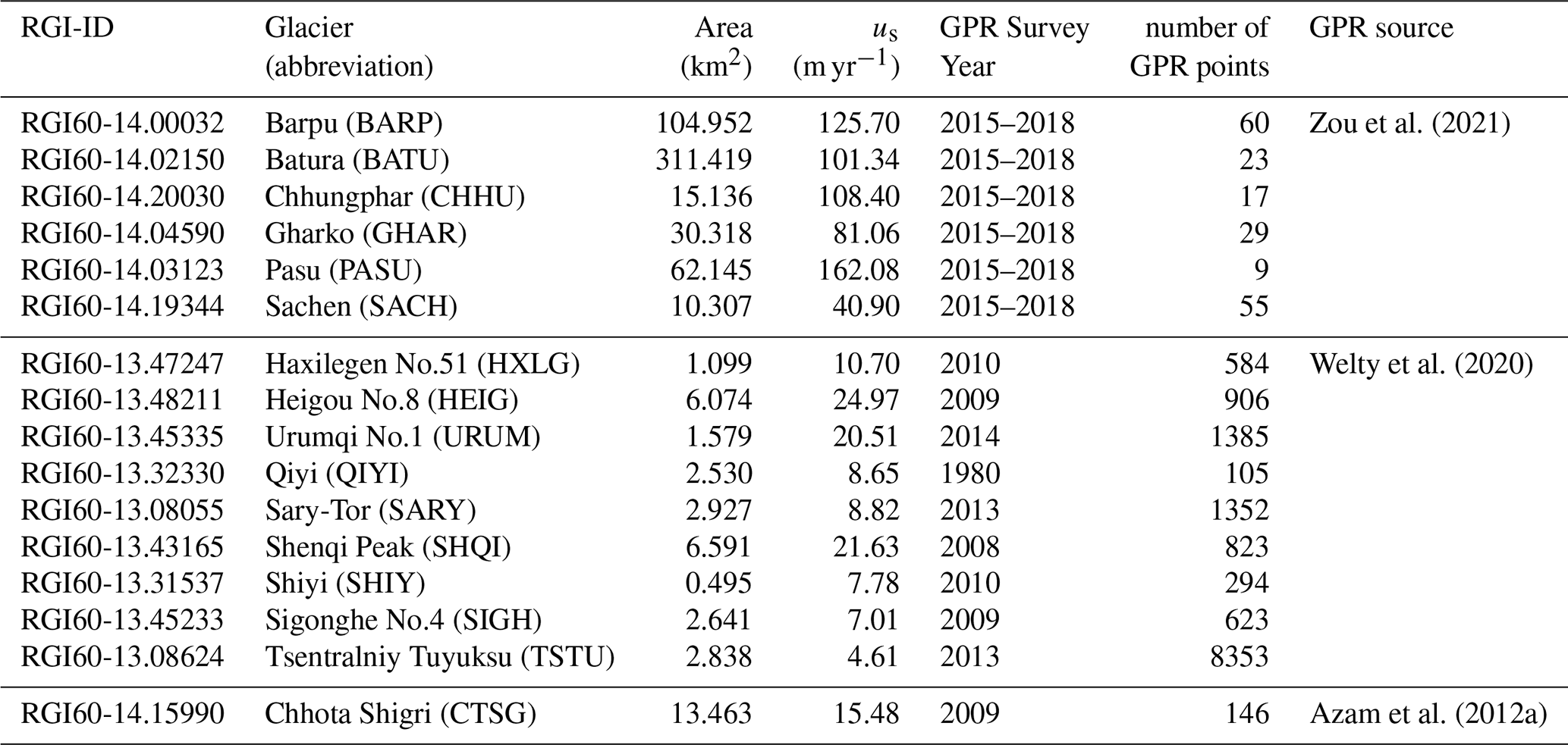
Glaciers in HMA are influenced by the Indian monsoon, westerlies, and East Asian monsoon (Bolch et al., 2012; Yao et al., 2012). These climatic regimes drive pronounced spatial heterogeneity in glacier distribution, mass balance, and dynamics (Hugonnet et al., 2021; Miles et al., 2021; Millan et al., 2022; Wang et al., 2023). For this study, we selected 16 glaciers spreading across the Tian Shan (7 glaciers), Himalayas (1 glacier), Qilian Shan (2 glaciers), and Karakoram (6 glaciers) (Fig. 1). The sample exhibit significant diversity in area, width, and surface velocity. Notably, one glacier covers less than 1 km², while 9 exceed 5 km² (Table 1). The Urumqi No. 1 Glacier (Tian Shan) bifurcated into eastern and western branches in 1993 (Wang et al., 2016); we analyze these branches as a single glacier.

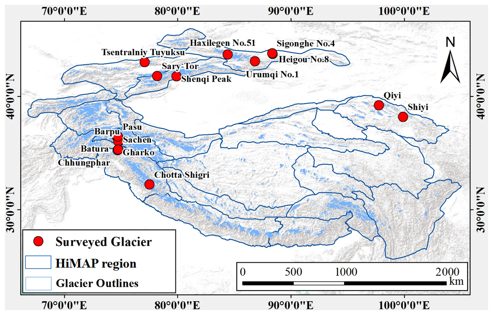
Figure 1 Distribution of HMA glaciers and the location of selected glaciers.

Table 1 Glaciers from RGI 6.0, survey years, and GPR data sources.

This study utilized glacier outlines from the Randolph Glacier Inventory version 6.0 (RGI 6.0; https://www.glims.org/RGI/, last access: 23 September 2021) (Pfeffer et al., 2014). Topographic features essential for ice thickness inversion—including surface slope and elevation – were derived from the Copernicus DEM GLOB-30 (hereafter COPDEM30; https://registry.opendata.aws/copernicus-dem, last access: 10 April 2022). COPDEM30 provides near-global coverage at 30 m resolution, generated through reprocessing of World DEM™ data acquired between 2011 and 2015. The reprocessing involved resampling, void filling, and replacement of anomalous elevation values (Becek et al., 2016; González-Moradas and Viveen, 2020; Hawker et al., 2022; Li et al., 2022). The Copernicus DEM exhibits an absolute vertical accuracy of 4 m and relative vertical accuracy of 2 m (Hawker et al., 2022). For computational efficiency in ice thickness modeling, COPDEM30 data were resampled to 50 m resolution.

Ice thickness models based on the SIA estimate glacier thickness using ice motion characteristics (Gantayat et al., 2014; Millan et al., 2022). This study utilizes glacier surface velocities from Millan et al. (2022), who derived ice flow velocities for 2017–2018 by applying sub-pixel correlation techniques to remote sensing imagery (Millan et al., 2019; Millan et al., 2022). The dataset features a spatial resolution of 50 m with a reported velocity uncertainty of 10 m yr⁻¹. Moreover, this dataset includes the standard deviations of ice velocity in the east–west and north–south components, which enables the computation of the standard deviation of ice velocity for each glacier. Based on the above data, we calculated the mean surface velocity for each glacier (Table 1).

To evaluate model-derived ice thickness accuracy, we collected GPR measurements from 16 glaciers. Data sources include the Glacier Thickness Database version 3 (GlaThiDa v3), maintained by the Global Terrestrial Network for Glaciers (GTN-G) through the World Glacier Monitoring Service (WGMS; https://wgms.ch/, last access: 27 February 2022), as well as published studies (Azam et al., 2012a; Welty et al., 2020; Farinotti et al., 2021). GlaThiDa represents a global compilation of ice thickness measurements obtained through GPR, drilling, and seismic methods (Welty et al., 2020). For our study glaciers, temporal inconsistencies between ice thickness measurements and DEM/outline acquisition dates are considered negligible (Li et al., 2022). However, the GPR measurements for the Qiyi Glacier date back to 1980. After more than half a century of change, the difference between the simulated ice thickness and the GPR measurements should be viewed with this long-term evolution in mind.

2.2 Ice thickness model considering basal sliding law (ITMSL)

Laminar flow equation is a fundamental in glacier dynamics (Cuffey and Paterson, 2010). It describes the glacier surface velocity as the sum of ice deformation and basal sliding (Gantayat et al., 2014; Wu et al., 2020):

$$\begin{array}{}\text{(1)}& u_{\mathrm{s}}=u_{\mathrm{b}}+{\displaystyle \frac{\mathrm{2}A}{n+\mathrm{1}}}{\mathit{\tau }}_{\mathrm{b}}^{n}H\end{array}$$

where u_s and u_b (m s⁻¹) are the surface and basal sliding velocity, respectively. n is Glen's flow law exponent, typically assumed to be 3. A is the creep parameter, dependent on ice temperature, fabric, grain size, and water content. Here we use $A=\mathrm{2.4}\times {\mathrm{10}}^{-\mathrm{24}}$ Pa⁻³ s⁻¹ (Cuffey and Paterson, 2010; Gantayat et al., 2014). H (m) is the ice thickness. τ_b (Pa) is the basal shear stress, calculated as (Li et al., 2012):

$$\begin{array}{}\text{(2)}& {\mathit{\tau }}_{\mathrm{b}}=f\mathit{\rho }gH\sin \mathit{\alpha }\end{array}$$

where ρ is the ice density, taken as a constant 900 kg m⁻³, g is the acceleration due to gravity (9.8 m s⁻²), α is the glacier surface slope (Farinotti et al., 2017, 2019). f is the valley shape factor, a dimensionless parameter accounting for the influence of glacier cross-sectional geometry on the relationship between driving stress and basal shear stress (Li et al., 2012; Ramsankaran et al., 2018). f is estimated using glacier width (w) and ice thickness (H):

$$\begin{array}{}\text{(3)}& f={\displaystyle \frac{\mathrm{2}}{\mathit{\pi }}}\arctan \left({\displaystyle \frac{w}{\mathrm{2}H}}\right)\end{array}$$

When using laminar flow equation to estimate glacier thickness, an assumption must be made regarding the ratio of basal sliding to surface velocity. Gantayat assumes this ratio to be 25 % (Gantayat et al., 2014), whereas Millan infers that this ratio ranges from 0.1 to 0.9 based on the relationship between surface slope and ice velocity (Millan et al., 2022).

There are three types of basal sliding laws for glaciers (Weertman, 1957; Budd et al., 1979; Schoof, 2005). Weertman derived a basal sliding law by modelling the glacier bed as uniformly distributed regular cubic obstacles (Weertman, 1957). This law incorporates two key mechanisms: pressure melting and enhanced ice creep, establishing a nonlinear relationship between basal sliding velocity, basal shear stress, and ice bed roughness (Weertman, 1957). However, Weertman's formulation neglects the influence of subglacial water content variations on sliding. To address this limitation, Budd introduced a sliding law accounting for basal cavity evolution, though it retains a power-law form (Budd et al., 1979; Fowler and Frank, 1981). Crucially, basal shear stress increases with sliding velocity until reaching a limit controlled by subglacial hydrology (Iken, 1981). As water pressure rises, basal drag approaches a maximum value determined by the maximum bed slope (Schoof, 2005; Gagliardini et al., 2007; Zoet and Iverson, 2020; Helanow et al., 2021; Gilbert et al., 2023). According to the Coulomb friction law, basal sliding velocity is positively correlated with basal shear stress and negatively correlated with effective pressure. Sliding accelerates once the shear stress exceeds the frictional threshold, with lower effective pressure further promoting motion. Nevertheless, the shear-stress-to-effective-pressure ratio, after peaking, declines with increasing sliding velocity and ultimately stabilizes (Zoet and Iverson, 2020; Helanow et al., 2021). We employ the Coulomb sliding law to characterize this complex interaction among water pressure, shear stress, and dynamics, which is given as follows (Helanow et al., 2021):

$$\begin{array}{}\text{(4)}& {\displaystyle \frac{{\mathit{\tau }}_{\mathrm{b}}}{N}}=C{\left({\displaystyle \frac{u_{\mathrm{b}}}{u_{\mathrm{b}}+A_{\mathrm{s}}{C}^n{N}^n}}\right)}^{\mathrm{1}/n}\end{array}$$

where N (Pa) is the effective pressure. Effective pressure is defined as the difference between ice overburden pressure and basal water pressure. Given the difficulty in precisely quantifying subglacial hydrological conditions, this study approximates the effective pressure as 0.9 times the ice overburden pressure (N = 0.9ρgHcos α). $C=\mathrm{0.84}\pm \mathrm{0.02}{m}_{max}$ is the maximum value of ${\mathit{\tau }}_{\mathrm{b}}/N$ (Gagliardini et al., 2007; Schoof, 2005). m_max is the maximum bedrock slope. A_s (m Pa⁻ⁿ yr⁻¹) is the sliding parameter. The sliding parameter A_s is defined as (Gagliardini et al., 2007):

$$\begin{array}{}\text{(5)}& A_{\mathrm{s}}=B\mathit{\lambda }+{\displaystyle \frac{-\mathrm{2}\times {\mathrm{10}}^{-\mathrm{5}}+\mathrm{0.013}r+\mathrm{0.0262}{r}^{\mathrm{2}}}{r^{\mathrm{2}}}}\end{array}$$

where $B=\mathrm{430}\pm \mathrm{40}$ MPa⁻³ yr⁻¹ is the ice fluidity parameter under isothermal conditions (Lliboutry, 1987); λ is the bedrock obstacle wavelength, which is calculated from the descent gradient of the subglacial topography using Fourier transform. r is the bedrock roughness coefficient (Gudmundsson, 1997; Schoof, 2005; Berends et al., 2023), calculated via root mean square height (RMSH) (Shepard et al., 2001; Berti et al., 2013):

$$\begin{array}{}\text{(6)}& r=\sqrt{{\displaystyle \frac{\mathrm{1}}{k-\mathrm{1}}}\sum _{i=\mathrm{1}}^k(z_i-\stackrel{\mathrm{‾}}{z}{)}^{\mathrm{2}}}\end{array}$$

where k is the moving windows size (number of cells), z_i is the cell elevation, and $\stackrel{\mathrm{‾}}{z}$ is the mean elevation within the window (Berti et al., 2013).

2.3 Accuracy assessment

This study evaluates three ice thickness models (Gantayat, Millan, ITMSL) applied to 16 HMA glaciers. Model performance is quantified using five statistical metrics: root mean square error (RMSE), standard deviation (SD), mean error (ME), relative error (RE), and correlation coefficient (CC) (Höhle and Höhle, 2009; Liu et al., 2019; Chen et al., 2022; González-Moradas and Viveen, 2020; Pang et al., 2023). These metrics are defined as:

$$\begin{array}{}\text{(7)}& {\displaystyle }\mathrm{RMSE}=\sqrt{{\displaystyle \frac{\sum _{i=\mathrm{1}}^n({\widehat{H}}_i-H_i{)}^{\mathrm{2}}}{n}}}\text{(8)}& {\displaystyle }\mathrm{SD}=\sqrt{{\displaystyle \frac{\sum _{i=\mathrm{1}}^n{\left({\widehat{H}}_i-H_i-\frac{\mathrm{1}}{n}\sum _{i=\mathrm{1}}^n({\widehat{H}}_i-H_i)\right)}^{\mathrm{2}}}{n-\mathrm{1}}}}\text{(9)}& {\displaystyle }\mathrm{ME}={\displaystyle \frac{\mathrm{1}}{n}}\sum _{i=\mathrm{1}}^n({\widehat{H}}_i-H_i)\text{(10)}& {\displaystyle }\mathrm{RE}={\displaystyle \frac{({\widehat{H}}_i-H_i)}{{\widehat{H}}_i}}\text{(11)}& {\displaystyle }\mathrm{CC}={\displaystyle \frac{\sum _{i=\mathrm{1}}^n\left(\left({\widehat{H}}_i-\frac{\mathrm{1}}{n}\sum _{i=\mathrm{1}}^n{\widehat{H}}_i\right)\left(H_i-\frac{\mathrm{1}}{n}\sum _{i=\mathrm{1}}^n{H}_i\right)\right)}{\sqrt{\sum _{i=\mathrm{1}}^n{\left({\widehat{H}}_i-\frac{\mathrm{1}}{n}\sum _{i=\mathrm{1}}^n{\widehat{H}}_i\right)}^{\mathrm{2}}}\sqrt{\sum _{i=\mathrm{1}}^n{\left(H_i-\frac{\mathrm{1}}{n}\sum _{i=\mathrm{1}}^n{H}_i\right)}^{\mathrm{2}}}}}\end{array}$$

where ${\widehat{H}}_i$ is the ice thickness measured by GPR at point i, H_i is the modelled ice thickness at point i, and n is the total number of GPR points.

RMSE quantifies the overall magnitude of errors between modelled and GPR measured ice thickness, serving as a composite measure of accuracy. SD of residuals characterizes the dispersion of model errors around their mean value, reflecting simulation stability. ME indicates systematic bias, with positive or negative values denoting overestimation or underestimation. RE expresses the absolute percentage deviation of modelled ice thickness from observations. CC measures the strength of linear relationship between modelled and measured thickness, where values approaching 1 indicate strong positive agreement. Collectively, these complementary metrics provide a comprehensive assessment of model performance in terms of accuracy, precision, bias, and consistency with observed spatial patterns.

3 Model Instructions

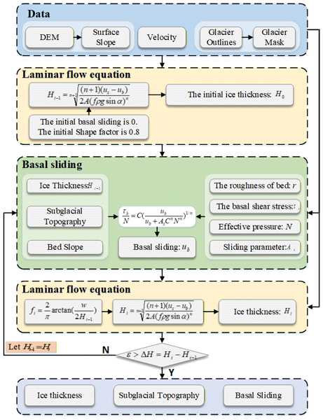
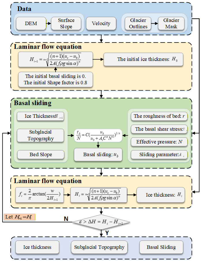
Model performance was validated using in situ ice thickness measurements from 16 glaciers across HMA. The experiments were driven by glacier surface velocities, topographic data, and glacier inventory. An initial simulation was conducted based on a set of assumptions, followed by iterative refinement until the results met the predefined convergence criteria. The iterative procedure for estimating glacier thickness using the ITMSL model comprises the following steps (Fig. 2):

1. Input Data: Provide the DEM, glacier surface velocity field, and glacier outlines.

2. Preprocessing: Extract the glacier mask from the outlines. Calculate the glacier surface slope (α) from the DEM, respectively. Initial u_b to 0.

3. Initial ice thickness: The initial value of shape factor is set to 0.8, and the initial ice thickness (H₀) is calculated using the laminar flow equation (Eq. 1).

4. Shape Factor Calculation: Determine glacier width (w) as the mean distance from the centerline to the glacier margins. Calculate the valley shape factor (f) using Eq. (3), incorporating w and H₀.

5. Basal shear stress: Bring f, H₀, α, and ice density (ρ) into Eq. (2) to derive τ_b.

6. Initial Bed Topography: Obtain the initial subglacial topography (Z₀) by subtracting H₀ from the surface DEM.

7. Sliding Law Parameters: Calculate the ice bed slope from Z₀. Calculate the maximum slope ratio (C) and bedrock roughness (r) (Eq. 6). Determine the sliding parameter (A_s) via Eq. (5). Estimate effective pressure (N) using H₀ and Z₀.

8. Basal Sliding Velocity: Put τ_b, N, C, A_s, and n into Eq. (4) for iterative calculation, thus obtaining u_b.

9. Updated Ice Thickness: Substitute the newly-obtained u_b into Eq. (1) to recompute ice thickness (H_i).

10. Convergence Check: Calculate the difference in glacier mean thickness between iterations: $\mathrm{\Delta }H=H_i-H_{i-\mathrm{1}}$. If ΔH is less than the threshold, the final glacier thickness and subglacial topography are output. Else, H_i is updated to H_i−1 and return to Step 3.

Figure 2 Flow chart of glacier thickness inversion using ITMSL model.

4 Model experiments

4.1 Calibration of ITMSL model

This study presents an ITMSL ice thickness model. To evaluate its performance, the model was applied to 16 HMA glaciers. In this study, the model parameters can be divided into two categories: those derived from glacier surface characteristics, such as shape factor and glacier width, and those derived from subglacial topography, including bed roughness, bed obstacle wavelength, and bed slope. Specifically, glacier width is calculated from glacier outline, while the shape factor is computed using both the glacier width and the initial ice thickness (Ramsankaran et al., 2018). Bed roughness is determined from subglacial topography (Berti et al., 2013), and the obstacle wavelength is obtained by applying a Fourier transform to the subglacial topography. These parameters are iteratively updated during the cyclic operation of the ITMSL model based on the results of the previous simulation. The sliding parameter A_s is calculated based on bed roughness, bed obstacle wavelength, and ice fluidity parameters (Gagliardini et al., 2007). The values of the ice fluidity parameter B (430±40 MPa⁻³ yr⁻¹) were initially adopted from the literature (Lliboutry, 1987). Given that the glaciers in this study are distributed across various regions of HMA, we expanded the parameter's range to 250–750 MPa⁻³ yr⁻¹ in order to obtain locally optimized values within a reasonable range. In addition, the parameter B has been calibrated using ice thickness measurements derived from GPR. We systematically tested B values at 5 MPa⁻³ yr⁻¹ interval to quantify its influence on thickness estimates, while other parameters were either literature-derived or glacier-specific. The optimal B value for each glacier was determined by minimizing SD between modeled and GPR measured thickness.

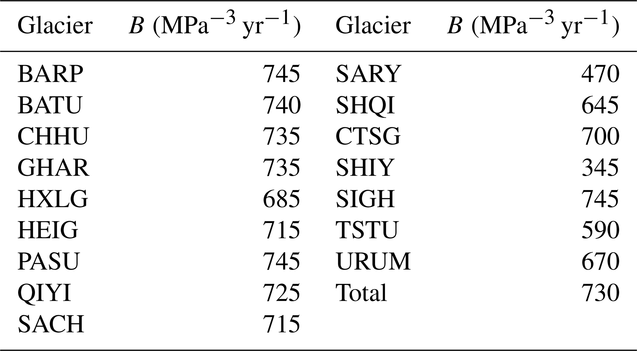
For the 16 selected glaciers, the calibrated optimal B values ranged 345–745 MPa⁻³ yr⁻¹, while the overall optimal value for all 16 glaciers is 730 MPa⁻³ yr⁻¹ (Fig. 3). 10 glaciers exhibited B exceeding 700 MPa⁻³ yr⁻¹, while SHIY, SARY, and TSTU showed values below 600 MPa⁻³ yr⁻¹. The Total B value for the 16 glaciers is determined by pooling all GPR measurement points together, calculating SD of the simulated ice thickness for different B values, and then selecting the B value that minimizes the SD as the global optimal value. These calibrated parameters provide reference values for regional ice thickness inversions in unmeasured HMA glacier (Table 2). It should be noted that the 16 glaciers investigated in this study are mainly distributed in the Tien Shan and Karakoram regions, with limited validation in the Indian monsoon-dominated Himalaya and southeastern Tibetan Plateau. Moreover, as shown in Fig. 3, the SD for some glaciers decreases monotonically with increasing B values, whereas other glaciers display irregular fluctuations. This indicates that the B value range is not universally suitable for all glaciers, potentially due to differences in glacier characteristics and climatic conditions. Therefore, caution is required when applying B = 730 MPa⁻³ yr⁻¹ to study glacier thickness and volume in these regions. Several factors contribute to variations in parameter values, including model itself, accuracy of input data, and potential inconsistencies in the timing of input data acquisition compared to GPR measurements.

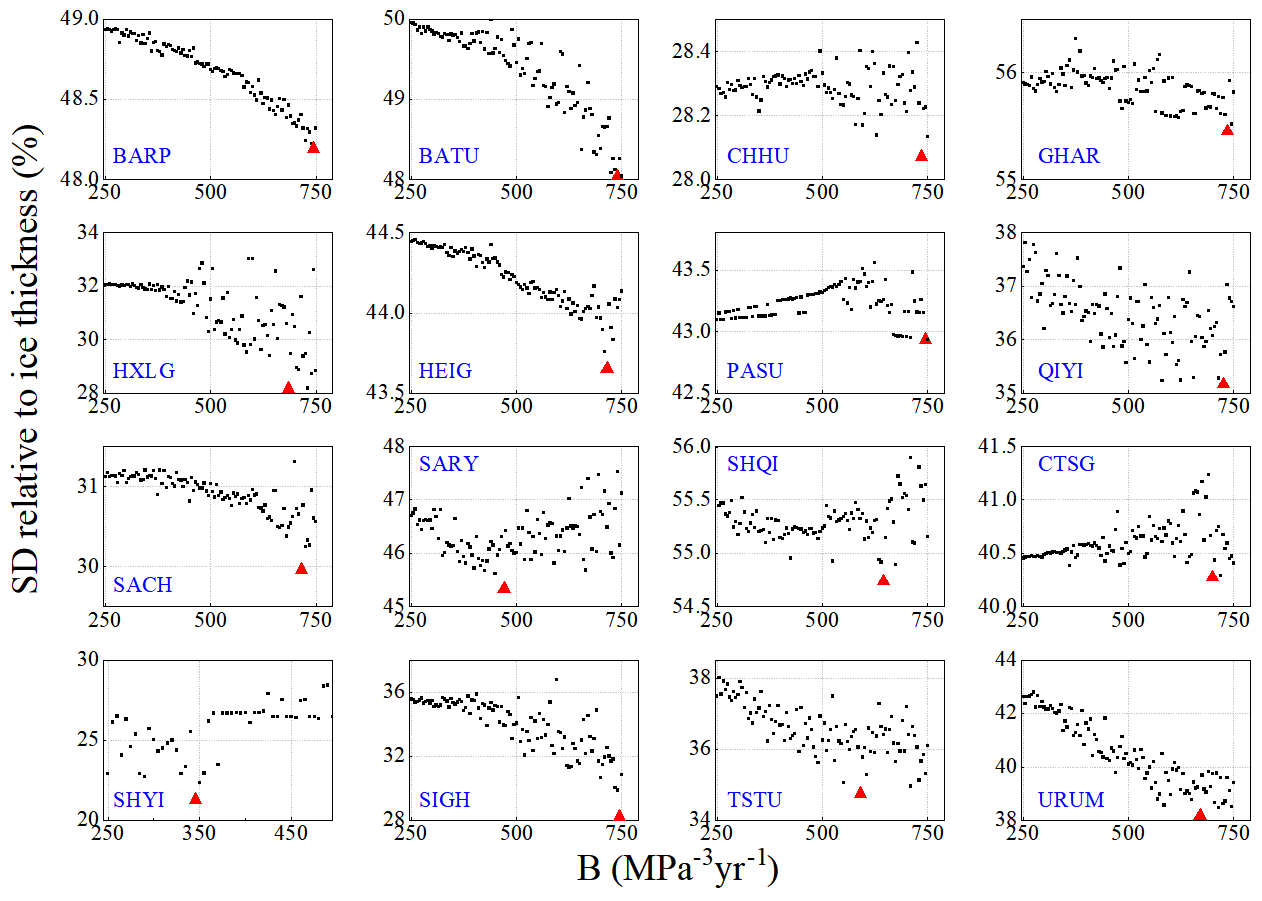
Figure 3 Ratio of the SD of ice thickness inversion to ice thickness for different values of parameter B in the ITMSL model.

Table 2 The optimal fluidity parameters of each glacier calculated by GPR.

4.2 Ice thickness distribution and subglacial topography

Using calibrated parameters, we applied the ITMSL model to estimate thickness distributions across the 16 study glaciers (Additional results are shown in Fig. S1 in the Supplement). For comparison, we also referred to the ice thickness estimates derived from the laminar flow equation-based Gantayat and Millan models (Gantayat et al., 2014; Millan et al., 2022). Among the 16 glaciers, CTSG is a widely studied glacier frequently used for ice thickness model validation (Frey et al., 2014; Azam et al., 2012b). Therefore, this study takes CTSG as an example to conduct a detailed analysis of ice thickness, subglacial topography, and basal sliding; the same procedure is applied to the remaining 15 glaciers. The mean ice thickness derived from the GPR validation points at the CTSG glacier is 172.88 m. The ITMSL model produced a mean thickness of 110.70 m and a total glacier volume of 1.4753 km³. Spatially, all three models (ITMSL, Gantayat, Millan) consistently captured characteristic thickness patterns: maximum along the central flowline and minimum in tributaries and marginal zones. In terms of mean ice thickness, ITMSL (110.70 m), Millan (104.90 m), and Gantayat (98.39 m) differ from one another, with Gantayat being the thinnest. Crucially, ITMSL exhibited closest agreement with GPR data, indicating superior accuracy relative to the comparison models.

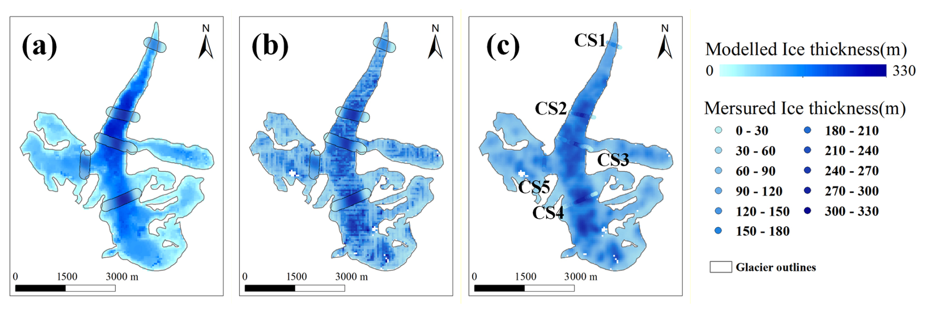
Figure 4 CTSG glacier thickness estimated by the three models. (a) Millan et al. (2022), (b) Gantayat et al. (2014), (c) ITMSL.

Figure 5 RMSE of CTSG glacier 5 cross-sections.

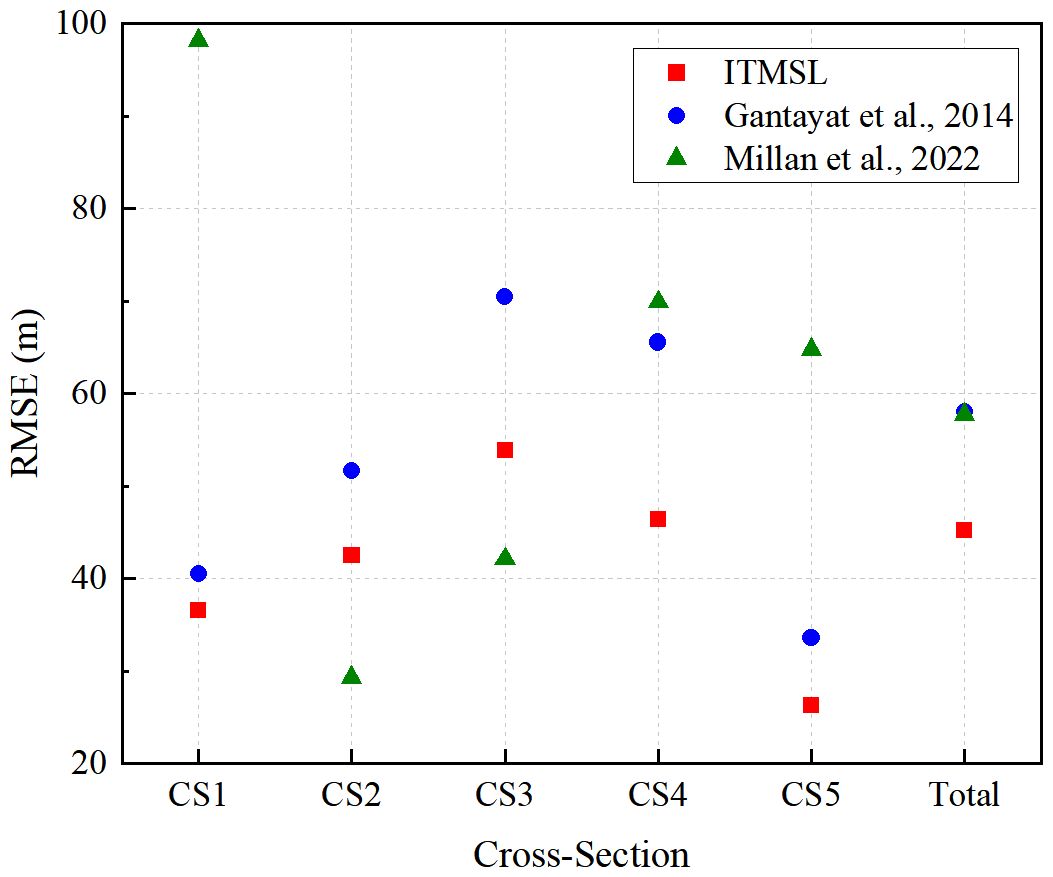
GPR surveys delineated 5 cross-sections (CS1-CS5) at CTSG glacier (Fig. 4; Additional results are shown in Figs. S2–S4). We evaluated ice thickness accuracy at each CS using RMSE for three models (Fig. 5; Additional results are shown in Table S1 in the Supplement). ITMSL demonstrated superior performance at CS1, CS4, and CS5 with RMSE values of 36.6, 46.5, and 26.3 m respectively, outperforming Gantayat (40.5, 65.6, 33.6 m) and Millan (98.2, 69.9, 64.8 m). Conversely, Millan achieved lower RMSE at central flowline sections CS2 (29.4 m) and CS3 (42.1 m), compared to ITMSL (42.5, 53.9 m) and Gantayat (51.7, 70.5 m).

Figure 6a reconstructs the subglacial topography of CTSG glacier by subtracting modelled ice thickness from the DEM-derived surface elevation (See Figs. S5–S7 for the subglacial topography, basal sliding, and basal sliding ratio of other glaciers.). The accuracy of this reconstructed bed topography is contingent upon the precision of both the ice thickness estimates and the input DEM. Analysis of basal sliding velocity reveals a glacier-wide mean of 5.68 m yr⁻¹ ($u_{\mathrm{b}}/u_{\mathrm{s}}=\mathrm{34.7}$ %), The quantified $u_{\mathrm{b}}/u_{\mathrm{s}}$ ratio further provides critical constraints on glacial dynamical behavior, underscoring its essential role in advancing ice thickness inversion methodologies.

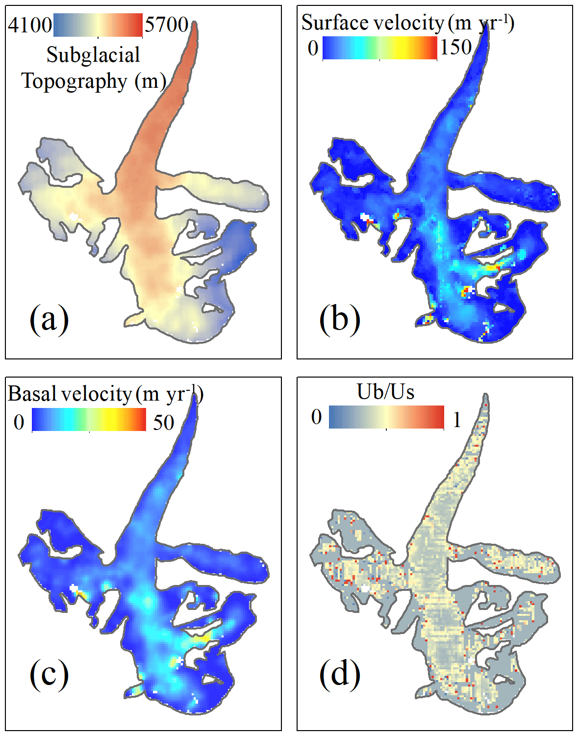
Figure 6 (a) CTSG glacier subglacial topography, (c) basal sliding, and (d) the ratio of sliding velocity to surface velocity inverted by ITMSL; (b) surface velocity used as input to ITMSL.

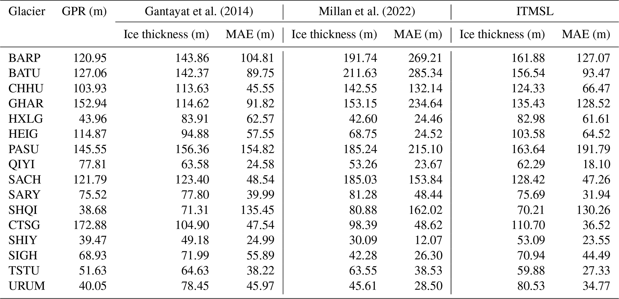
We applied the ITMSL model to estimate ice thickness and basal sliding velocity across the selected glaciers (Table 3; Additional results are shown in Fig. S6). Modeled ice thickness values represents point-specific averages collocated with GPR measurements. Results indicate systematic overestimation for 12 glaciers and underestimation for four. This bias arises from inherent limitations in laminar flow equation parameterization. The ratio $u_{\mathrm{b}}/u_{\mathrm{s}}$ ranges from 0.258 to 0.355, exceeding the value of 0.25 assumed by Gantayat et al. (2014). It is worth noting that, although the mean ice thickness estimated by our model is slightly higher than that of the other two models, it achieves a superior MAE. This indicates that our model captures the mechanical coupling between surface velocity and ice thickness more effectively and exhibits greater resilience to data noise, thereby substantially reducing extreme outliers. Nevertheless, the systematic overestimation in the mean estimates suggests that the current physical parameterization does not fully account for the diversity of subglacial hydrological conditions across the study area, leading to a general upward bias. Unlike the competing models, whose favorable mean performance stems from mutual error cancellation, our model produces a more structured error distribution, making it better suited for regional-scale ice-thickness inversion. Consequently, incorporating the physically-based sliding law enhances laminar flow equation by explicitly representing subglacial processes, thereby improving regional ice thickness estimation accuracy.

Table 3 Comparison of mean ice thickness from GPR measurements and retrievals by three models (Gantayat, Millan, ITMSL), along with their respective mean absolute errors (MAE), for the 16 glaciers.

4.3 Accuracy assessment of the glacier thickness

Comprehensive evaluation of the ITMSL model against Gantayat, Millan using 5 statistical metrics applied to GPR-measured thickness data (Fig. 7) demonstrates significant improvements: ITMSL achieves higher correlation coefficients between the modelled and GPR-measured ice thickness than Millan in 9 of 16 glaciers, and surpasses Gantayat in 13 of 16, indicating stronger linear relationships with the observed data; reduces SD to 39.12 m (32.65 % lower than Millan's 58.08 m and 20.62 % below Gantayat's 49.28 m), with particularly notable decreases at BATU (61.01 % lower than Millan) and CHHU (45.75 % lower than Millan); and achieves 21.58 % lower RMSE (53.59 m) than Millan (68.34 m) and 17.46 % reduction versus Gantayat (64.92 m). Although 4 glaciers (SHIY, HXLG, URUM, HEIG) exhibit higher deviation in ice thickness inversion using ITMSL compared to Millan et al. (2022) (see RMSE, ME, and RE in Fig. 7), the overall accuracy of ITMSL remains superior to that of both Millan et al. (2022) and Gantayat et al. (2014) across the majority of the 16 glaciers, confirming its reliability. Regarding RE, except for an outlier on the SHQI glacier, the RE values of the remaining 15 glaciers are relatively similar: −2.48 to 0.2 for Millan et al. (2022), −1.86 to −0.02 for ITMSL, and −1.85 to 0.02 for Gantayat et al. (2014). The overall mean RE values for these 16 glaciers are −1.81, −1.53, and −1.72, respectively. In terms of ME, the ranges of ME for the 16 glaciers inverted by the three models are −277.69 to 19.72 (Millan et al., 2022), −191.79 to 4.92 (ITMSL), and −135.42 to 7.26 (Gantayat et al., 2014), with overall mean ME values of −36.01, −36.63, and −42.27 m, respectively. In this study, both Mean Error (ME) and Relative Error (RE) are defined as “GPR-measured minus model-simulated values”. A positive value thus indicates that the model underestimates the observed ice thickness, whereas a negative value indicates overestimation. Both ME and RE indicate that the inversion results from the three models are generally higher than the GPR-measured ice thickness, suggesting that the model input data and parameter calibration still have room for improvement. Correlation analysis between the model-inverted thickness and GPR-measured ice thickness yields overall correlation coefficients of 0.29 (Millan et al., 2022), 0.53 (ITMSL), and 0.42 (Gantayat et al., 2014). These advances stem directly from the physically constrained basal sliding parameterization, which effectively mitigates Gantayat's problematic $u_{\mathrm{b}}/u_{\mathrm{s}}$ assumption of 0.25 that systematically overestimates thickness. Compared with other ice thickness models also based on the laminar flow equation, ITMSL achieves improved accuracy in glacier thickness inversion studies.

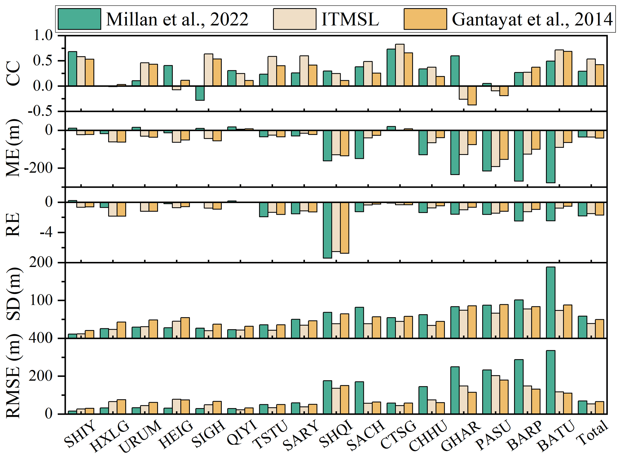
Figure 7 Comparison of ice-thickness inversion accuracy among three SIA-based models (Millan, Gantayat, ITMSL), referenced against GPR measurements. Metrics: correlation coefficient (CC), mean error (ME), relative error (RE), standard deviation (SD), and root mean square error (RMSE). All axis abbreviations are defined herein.

Despite inherent limitations in input data quality and model parameterization, the ITMSL model demonstrates robust performance across diverse HMA glaciers (Fig. 7), though localized discrepancies persist in topographically complex regions. Inter-model variations primarily arise from uncertainties in foundational datasets, particularly DEM precision, surface velocity accuracy, and slope derivation errors. Crucially, the convergence of ITMSL with established models (Gantayat and Millan) validates its utility as a physically constrained framework for regional glacier thickness distribution mapping. Estimation accuracy can be further enhanced through integration of multi-temporal velocity products, optimization of sliding law parameters, and assimilation of subglacial topography constraints.

5 Discussion

5.1 Influence of Surface Velocity on Ice-Thickness Model Performance

To evaluate the applicability of various ice-thickness inversion models to glaciers with different surface velocity, we classified surface velocity into intervals of 5 m yr⁻¹ and calculated the ice thickness bias, RMSE for the models of Millan et al. (2022), Gantayat et al. (2014), and our proposed ITMSL, as well as the RMSE differences of ITMSL relative to the other two models (Fig. 8). The results show that the ice-thickness bias of all three models increases approximately linearly with surface velocity, with R² of 0.76, 0.78, and 0.87, respectively.

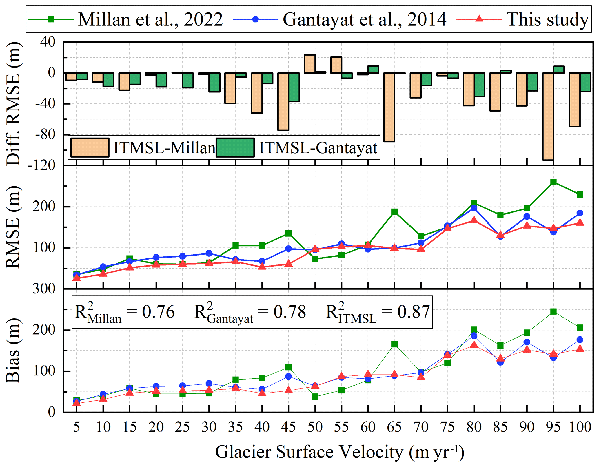
Figure 8 Comparison of ice-thickness inversion bias, root-mean-square error (RMSE), and their differences among ITMSL, Gantayat, and Millan models across surface velocity intervals.

In the low-velocity regime (≤50 m yr⁻¹), ITMSL consistently yields lower RMSE than the Millan and Gantayat models, and the biases relative to GPR measurements remain relatively small for all models. However, when surface velocity exceeds 70 m yr⁻¹, both bias and RMSE rise to over 100 m. Analysis of the RMSE differences reveals that, with increasing velocity, ITMSL exhibits a progressively larger advantage over Millan. In contrast, the difference relative to Gantayat shows a two-stage pattern: below 50 m yr⁻¹, the difference increases with velocity; around 50 m yr⁻¹, ITMSL performs comparably to or slightly worse than Gantayat; and beyond that threshold, the difference resumes its upward trend. Overall, ITMSL outperforms or matches the existing models across most velocity intervals, with only a narrow transitional zone (∼50 m yr⁻¹) where it is on par with Gantayat. These findings confirm the robustness and demonstrated superiority of ITMSL under varying flow conditions.

5.2 Analysis of factors affecting the accuracy of simulated ice thickness

Using glacier-specific characteristics, we iteratively computed key parameters, including the valley shape factor (f), effective stress (N), basal sliding velocity (u_b), sliding parameter (A_s), and bedrock roughness (r), to derive ice thickness distributions across the 16 glaciers. Although ITMSL demonstrated improvements, localized accuracy deficits at 4 glaciers (SHIY, HXLG, URUM, HEIG) necessitate targeted analysis. Ice thickness model accuracy is governed by 4 factors: (1) input data quality (DEM, surface velocity, glacier outline); (2) model limitations; (3) parameterization uncertainties; and (4) glacier characteristics (slope, aspect, bedrock topography) (Frey et al., 2014; Pang et al., 2023; Wang et al., 2023). For URUM glacier, analyzed as an integrated system incorporating both eastern and western branches (Wang et al., 2016), we quantified performance using SD.

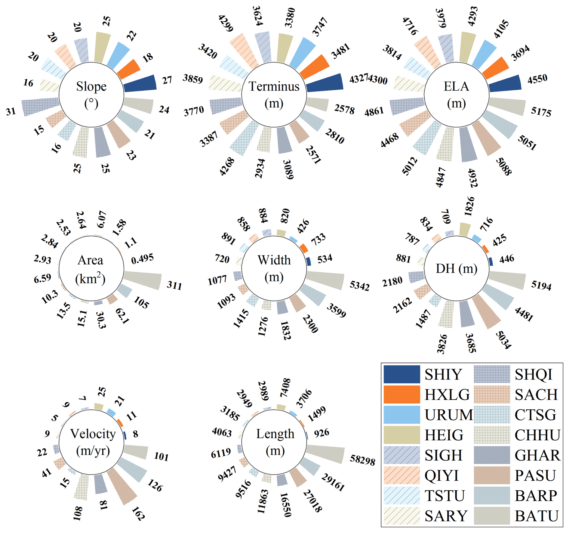
Figure 9 Characteristics of glacier surface slope, terminus elevation, equilibrium line altitude, area, mean width, difference in height (DH), ice velocity, length.

Statistical analysis of glacier geometry and dynamics (Fig. 9) revealed distinct characteristics for 4 glaciers that showed limited improvement in accuracy: SHIY (length: 926 m, area: 0.495 km², width: 534 m), HXLG (length: 1499 m, area: 1.099 km², width: 733 m), and the eastern branches (URUME; length: 2012 m, area: 1.03 km², width: 513 m) and western branches (URUMW; length: 1694 m, area: 0.55 km², width: 322 m) of the URUM glacier. While sharing comparable elevation, velocity, and slope characteristics with other glaciers, their small size exacerbates four key limitations. First, reduced glacier dimensions challenges ice thickness inversion due to insufficient grid resolution. Second, spatial resolution mismatches between modelled ice thickness (50 m cells) and GPR point spacing (1.5–5 m) amplify errors. Third, the reliability of velocity monitoring for small glaciers is low, and basal sliding is weak or absent, making effective simulation difficult. Finally, inherent model uncertainties in ice density parameterization, sliding coefficient calibration, and bedrock roughness estimation contribute to inaccuracies. Consequently, the thickness results obtained from these four small glaciers also highlight the limitations and applicable conditions of the ITMSL. Addressing these multiscale challenges, spanning data acquisition, model structure, and parameter sensitivity, remains essential for enhancing ITMSL's reliability across diverse glacial regimes.

5.3 Influence of glacier basal sliding on the ice thickness

This study combines the basal sliding law with the laminar flow equation to develop the ITMSL model (Schoof, 2005; Gantayat et al., 2014; Zoet and Iverson, 2020; Millan et al., 2022). At each GPR measurement point, we computed the $u_{\mathrm{b}}/u_{\mathrm{s}}$ ratio using the ITMSL model. Based on this ratio, we binned the points into two regimes: 0.1–0.4 and 0.4–1.0. The comparative analysis at these GPR points (Fig. 10) reveals distinct performance regimes: for the 0.1–0.4 bin, ITMSL outperformed other models in terms of quartiles and outliers; for the 0.4–1.0 bin, ITMSL reduces the absolute deviation relative to both Gantayat and Millan. Crucially, the overall ice thickness deviation of ITMSL was 13.35 % lower than that of Gantayat and 0.2 % lower than that of Millan.

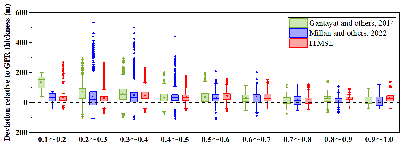
Figure 10 Comparative analysis of ice thickness estimation deviations for different ratios of basal sliding to surface velocity.

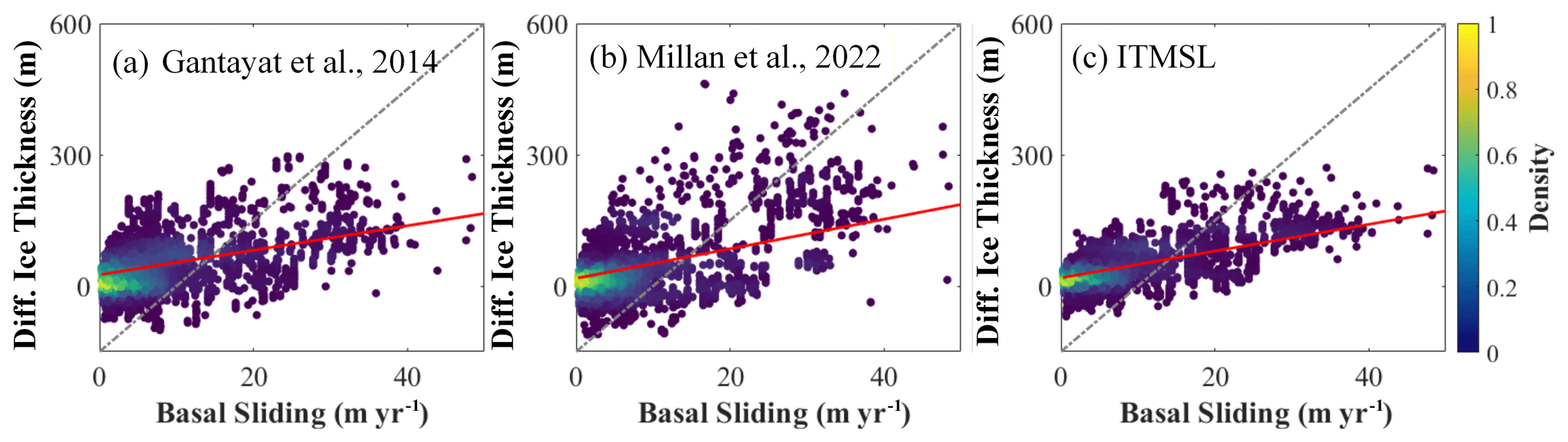
Figure 11 Deviations of ice thickness estimates from three laminar flow models at different basal sliding. (a) Gantayat; (b) Millan; (c) ITMSL.

Beyond model intercomparison, we analyze the effects of basal sliding velocity on ice thickness estimation (Fig. 11). The correlation coefficients between ice thickness bias and u_b are 0.4572 for Gantayat, 0.468 for Millan, and 0.6291 for ITMSL. ITMSL can reasonably capture the spatial variation of basal sliding and thereby improve the physical consistency of ice thickness estimates, whereas other models that ignore sliding cannot reflect this key dynamical process. This enhanced physical responsiveness validates the efficacy of integrating basal drag constraints into laminar flow equation. Consequently, this integration significantly improves the robustness of thickness estimation across diverse glacial conditions.

5.4 Comparison with existing ice thicknesses

In this study, we evaluate the accuracy of the ITMSL model within the framework of the ITMIX. First, compare the ice thickness results calculated by each model. To place the ITMSL, Gantayat, and Millan models within a broader glaciological model framework, their thickness estimates are compared with four established models, namely Composite, GlabTop2, H-F, and OGGM (Huss and Farinotti, 2012; Frey et al., 2014; Farinotti et al., 2019; Maussion et al., 2019). The thickness data for these models are derived from Farinotti et al. (2019), whose methodological foundations include the mass conservation approach (OGGM, H-F), the shallow ice approximation theory (GlabTop2), and the weighted multi-model ensemble (Composite).

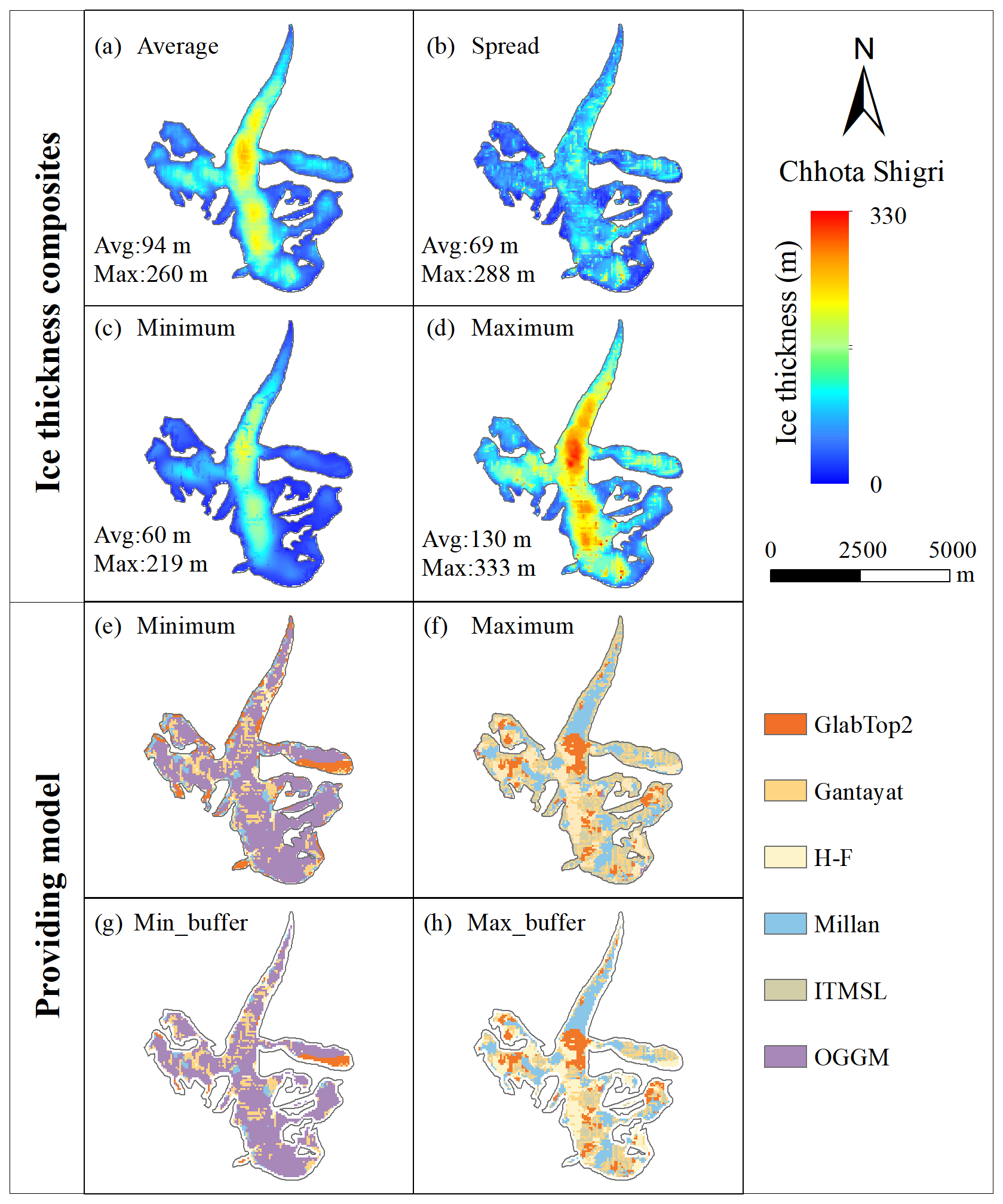
Figure 12 Comparison of simulated ice thickness among models. The first four panels present composite results from the models: (a) average, (b) spread, (c) minimal, and (d) maximal ice thickness distribution. The models corresponding to the minimum and maximum ice thickness at each pixel are shown in (e) and (f), respectively; Models corresponding to the minimum (g) and maximum (h) ice thickness at each pixel after excluding the 3×30 m buffer zone.

Taking the CTSG glacier as an example, we compare the composite mean ice thickness (i.e., the ice thickness distribution obtained by averaging, Fig. 12a) with the ice thickness spread (i.e., the spread of all model results within a pixel, Fig. 12b). Figure 12c and d present the maximum and minimum ice thickness composites, respectively, illustrating the composition of the composite results. The models producing the most extreme results are shown in Fig. 12e and f. For the CTSG glacier, the minimum ice thickness is predominantly provided by the OGGM model (62.17 %), while the minimum values from GlabTop2 are mainly distributed over the glacier's tributaries. In contrast, the maximum ice thickness is primarily contributed by ITMSL (27.69 %), Millan (22.35 %), Gantayat (20.91 %), and H-F (16.97 %). This pattern is consistent with the trends observed in the ITMIX results. Specifically, the maximum ice thickness from ITMSL is concentrated along the glacier margins; that from Millan is concentrated in the lower reaches and the tongue of the glacier; that from Gantayat is relatively evenly distributed; and that from the H-F model is concentrated in the upper reaches.

As described above, in the ITMSL data processing workflow, ice bed roughness is quantified using the RMSH method with a 3×3 pixel moving window. This configuration is likely the primary cause of the extreme errors observed at glacier margins in the ITMSL outputs. To mitigate boundary effects, we applied a buffer distance of 3×30 m to exclude marginal pixels (Fig. 12g and h). After this exclusion, the proportions of minimum extreme values among the models' thickness estimates over interior pixels rank as follows: ITMSL (0.25 %) < H-F (2.38 %) < Millan (3.75 %) < GlabTop2 (3.91 %) < Gantayat (15.45 %) < OGGM (74.28 %); while the maximum extreme values rank as: OGGM (0.11 %) < GlabTop2 (14.71 %) < ITMSL (15.14 %) < H-F (21.21 %) < Gantayat (21.76 %) < Millan (27.06 %). These results indicate that, although ITMSL yields relatively large errors at glacier margins, its thickness estimates for interior pixels are more concentrated and reasonable.

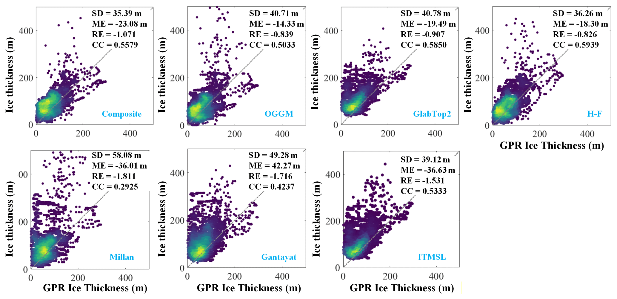
Figure 13 Evaluation of model-inverted ice thickness accuracy using GPR-measured ice thickness.

Comprehensive accuracy assessment reveals consistent ice thickness overestimation across all models, though ITMSL effectively constrains Millan's excessive deviations as evidenced by thickness distributions (Fig. 13). The ME quantification confirms a systematic positive bias. Farinotti et al. (2021) emphasized that no single model clearly outperforms all others, highlighting the advantage of multi-model ensembles over individual approaches. Compared to OGGM, the Composite model reduces thickness errors by 13.1 %; by 13.2 % relative to GlabTop2; by 2.4 % relative to H-F; by 39.1 % relative to Millan; by 28.2 % relative to Gantayat; and by 9.5 % relative to ITMSL. These findings validate multi-model ensemble approaches for leveraging complementary strengths through error compensation mechanisms, though absolute accuracy requires further enhancement given persistent overestimation trends.

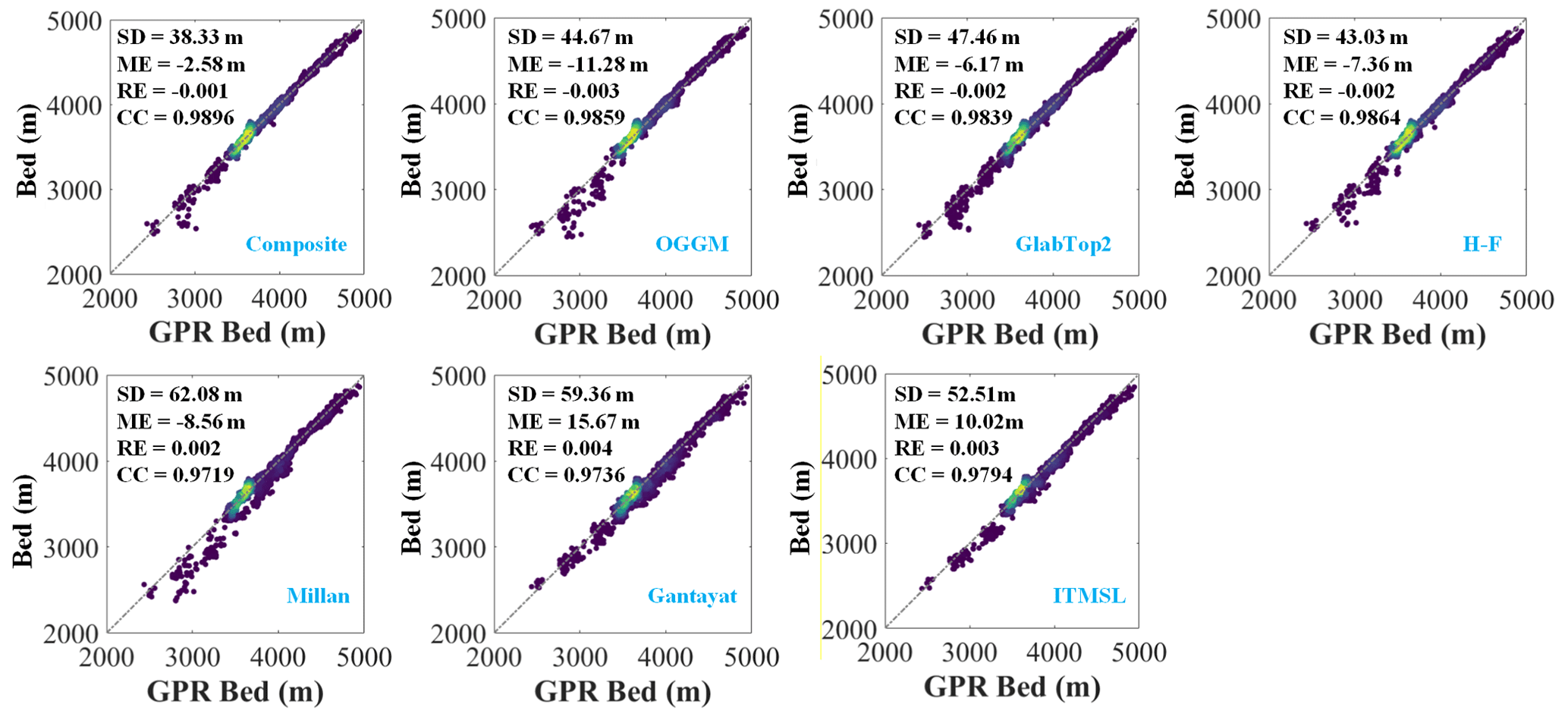
Figure 14 Evaluation of model-inverted subglacial topography accuracy using ice-bed measurements.

Subglacial topography was reconstructed by subtracting modelled ice thickness from GLOB30 surface elevations, with validation against GPR-derived bed measurements (Fig. 14). There is a discrepancy between the two: the former is the bed elevation indirectly derived from the inverted ice thickness, while the latter is obtained by subtracting the measured ice thickness from the surface elevation that was concurrently recorded during the thickness survey, yielding the bed elevation at each measurement point. The modeled and observed ice beds show excellent agreement, with correlation coefficients exceeding 0.97 across all seven models and relative errors below 0.4 %. The high-fidelity reproduction of basal geometry – achieved despite complex subglacial terrain – confirms the robustness of inversion methodologies for applications requiring precise bed mapping, particularly potential glacial lake research.

6 Conclusions and perspectives

This study presents a novel glacier thickness inversion model, ITMSL, which enhances traditional laminar flow equation by incorporating a physically-based basal sliding law. Applied to 16 glaciers across High Mountain Asia (HMA), ITMSL model autonomously estimates basal sliding velocity, ice thickness distribution, and subglacial topography with significantly improved accuracy – reducing SD by 20.62 % compared to Gantayat and 32.65 % versus Millan. This study highlighted the importance of considering glacier basal sliding in ice thickness estimates, particularly when $u_{\mathrm{b}}/u_{\mathrm{s}}$ is greater than 0.4. Although ITMSL exhibits robust performance on glaciers larger than 1 km², its performance degrades on smaller glaciers. Previous studies have demonstrated that multi-model ensemble approaches offer significant advantages in ice thickness inversion. Therefore, ITMSL should be used as a member of such an ensemble, rather than as a replacement for other methods.

With the growing availability of high-resolution remote sensing data, ITMSL shows great potential for glacier thickness estimation. However, the ITMSL does not account for the effects of glacier temperature and surface debris on ice thickness estimation, and lacked verification of modeled glacier sliding measurements. Despite these limitations, ITMSL model establishes a promising foundation for estimating ice thickness in complex mountain environments, particularly where traditional SIA assumptions prove inadequate.