A deep learning framework for gridding daily climate variables from a sparse station network

High-resolution gridded climate datasets are essential for Earth system modelling and impact assessments, yet generating them from sparse, irregularly distributed station networks remains a significant challenge, particularly in regions with complex topography. This study evaluates the Spatial Multi-Attention Conditional Neural Process (SMACNP), a probabilistic deep learning framework, for the daily spatial interpolation of air temperature and precipitation, marking the first application of its localized encoder variant to the challenge of gridding climate data from a sparse station network. We investigate two distinct encoder configurations – Global and Localized – to determine the optimal structural prior for capturing spatial dependencies in data-scarce regimes. The models were developed and evaluated using data from a sparse network of meteorological stations in Romania from 2020 to 2023. To ensure applicability for long-term historical reconstruction, the input features were restricted to static topographic predictors derived from a Digital Elevation Model (DEM). Performance was benchmarked against Regression Kriging (RK), a standard geostatistical baseline that incorporates these same topographic covariates. Results demonstrate that the SMACNP architectures substantially outperform the RK baseline for both variables. The SMACNP (Localized) configuration, which utilizes an attention mechanism, emerged as the most robust model, achieving the lowest Mean Absolute Error (MAE) and the highest correlation across the majority of seasons. The performance gains were particularly pronounced for precipitation, where the deep learning models effectively captured fine-scale spatial heterogeneity and non-linearities that traditional methods tended to over-smooth. Furthermore, the SMACNP framework demonstrated superior uncertainty quantification; while RK exhibited significant overconfidence in precipitation estimates, the SMACNP (Localized) model produced well-calibrated probabilistic predictions with near-ideal empirical coverage. These findings indicate that localized neural process-based models offer a powerful, scalable, and physically plausible alternative to geostatistical methods for generating high-quality gridded climate datasets in complex, data-sparse environments.

1 Introduction

Daily gridded climate datasets are essential inputs for a wide range of models and impact assessments. Producing these fields from sparse, irregularly distributed station networks remains challenging, especially over complex terrain (Hijmans et al., 2005). Air temperature tends to vary smoothly with controls such as elevation and latitude, whereas precipitation is intermittent, highly skewed, and spatially and temporally discontinuous (Daly et al., 1994). This problem is particularly critical in areas characterized by complex topography, where local factors like elevation and wind exposure introduce nonstationary relationships and heterogeneous spatial dependencies that challenge traditional geostatistical assumptions (Diggle and Ribeiro, 2007). Classical interpolators such as inverse distance weighting and kriging – including regression kriging (RK) – are widely used baselines (Hengl et al., 2007; Li and Heap, 2014). Their performance can degrade where covariance structure is nonstationary or relationships with covariates are nonlinear, conditions common in topographically complex regions. While machine-learning approaches, particularly tree ensembles such as random forest and gradient boosting, often improve accuracy by leveraging rich covariates (e.g., satellite products, elevation, and reanalysis fields), they can still be limited in modeling the most complex spatial dependencies (Appelhans et al., 2015; Iwase and Takenawa, 2024; Sekulić et al., 2021).

Deep learning (DL) provides a powerful alternative, offering flexible, data-driven representations capable of modelling the complex spatial and temporal non-linear relationships inherent in climate data (Reichstein et al., 2019). Conditional Neural Processes (CNPs), for instance,  learn distributions over functions from context points while providing uncertainty estimates (Garnelo et al., 2018). The convolutional variant, the Convolutional Conditional Neural Process (ConvCNP), uses translation-equivariant, continuous convolutions to capture local spatial dependencies and is well suited to gridded queries (Gordon et al., 2019; Vaughan et al., 2022). Attentive Neural Processes build on this by introducing cross-attention from target queries to context points, improving the handling of heterogeneity among observations (Kim et al., 2019). In parallel, Transformers, originating in natural language processing and later adapted to vision, provide a direct solution for leveraging rich covariate information from irregularly spaced stations. They use attention so each element can weight all others when forming its representation (Dosovitskiy et al., 2020; Vaswani et al., 2017). In spatial problems, this means that when geographic coordinates and relevant covariates (e.g., elevation) are encoded, a query at a target location can up-weight both nearby and distant stations that are most informative (e.g., those at similar elevation), directly addressing a key weakness of traditional distance-based interpolators. The Spatial Multi Attention Conditional Neural Process (SMACNP) exemplifies this approach by combining cross-attention from target queries to context stations with specialized spatial and feature-wise attention to capture distance-dependent structure and predictor correlations for interpolating point measurements (Bao et al., 2024b). Building on this, Gridded Transformer Neural Processes (GriddedTNP) were recently introduced to tackle the scalability issues of Transformer Neural Processes (TNPs) for large, unstructured spatio-temporal datasets like weather data, by employing specialized gridded pseudo-tokens for efficient attention (Ashman et al., 2024). Similarly, Graph Neural Processes (GNPs) combine Graph Neural Networks (GNNs) with Neural Processes (NPs) to explicitly model relationships and dependencies defined by a graph structure (Carr and Wingate, 2019). Taking a different structural approach, Bao et al. (2024a) introduced a two-stage framework, the Location-Embedded Graph Neural Networks-Residual Neural Processes (LEGNN-RNP), in which a graph neural network enhanced by self-attention-based location embeddings generates an initial prediction, while a subsequent residual neural process models the spatial structure of the remaining errors, refining the final prediction and quantifying uncertainty in a manner similar to RK.

Despite these architectural advancements, the application of such probabilistic deep learning frameworks to extremely sparse observation networks in regions with complex topography remains under-explored. Our preliminary experiments in this specific context revealed that alternative architectures, such as the ConvCNP and GriddedTNP, struggled to generalize effectively when relying solely on static topographic predictors. We present a case study evaluating the SMACNP deep learning architecture for gridding daily temperature and precipitation over Romania from a sparse national station network (156 stations). Romania provides a challenging testbed combining complex Carpathian topography, sparse and irregular station coverage, and mixed precipitation regimes. While the methodology is general and transferable to other regions with similar data availability, the evaluation presented here is specific to Romania and should be interpreted accordingly. To the best of our knowledge, this represents the first application of the SMACNP architecture, specifically its localized encoder variant, to the challenge of gridding daily climate data from a sparse observation network. Performance is compared with Regression Kriging (RK), which serves as the geostatistical baseline, for the period 2020–2023. The contributions of this study are: (i) a systematic evaluation of the SMACNP architecture for daily climate gridding over complex terrain, demonstrating its advantage over RK for both temperature and precipitation; (ii) a comparison of global and localized attention configurations, showing that restricting attention to spatial neighbours improves interpolation from sparse, irregular networks; and (iii) a comprehensive uncertainty assessment including probabilistic calibration, precipitation occurrence skill, and climate-relevant extreme indices.

The remainder of this paper is structured as follows. Section 2 describes the datasets employed and the preprocessing procedures. Section 3 outlines the methodological framework, including a detailed description of RK and SMACNP, and presents the experimental setup. Section 4 reports the results, with a focus on interpolation accuracy and predictive uncertainty. Finally, Sects. 5 and 6 discuss and summarize the main findings and provide concluding remarks. Our focus is on spatially aware probabilistic DL models (SMACNP and its variants) that natively handle irregular station sets and provide calibrated uncertainties. Our formal comparison focuses on RK as the geostatistical reference and on the neural-process architectures considered in this study. The conclusions are therefore restricted to these evaluated methods and should not be interpreted as a general comparison with all machine-learning interpolation approaches.

2 Study area and data

The study is conducted over Romania, a region characterized by complex topography including the Carpathian Mountains, plateaus, and plains. We use daily meteorological station data and a topographic variable extracted from high-resolution Digital Elevation Model (DEM) to develop and evaluate the interpolation models.

2.1 Meteorological and topographic datasets

The primary dataset consists of daily homogenized mean air temperature (°C) and total precipitation (mm) from a network of meteorological stations across Romania, spanning 2020–2023. The complete dataset and associated station metadata can be accessed through the Zenodo repository (Dumitrescu, 2025). While the experiments in this study are conducted on this recent period, the proposed method is ultimately intended for application to the full long-term dataset covering 1901 to the present (Dumitrescu et al., 2025). The station data are pre-partitioned into a training set (130 stations), used for model development and validation, and a held-out test set (26 stations), used exclusively for final performance evaluation for all the models selected in the study (Fig. 1). To ensure strict evaluation integrity, the 26 test stations were selected randomly once before any model development and remained fixed throughout the study. These 26 stations were completely excluded from the training pool. The available days were split temporally into 80 % for training and 20 % for validation (early stopping and model selection). The final evaluation was performed across all days in the 2020–2023 period by conditioning on the 130 training-pool stations and predicting exclusively at the 26 held-out test stations, ensuring a strict spatial out-of-sample evaluation.

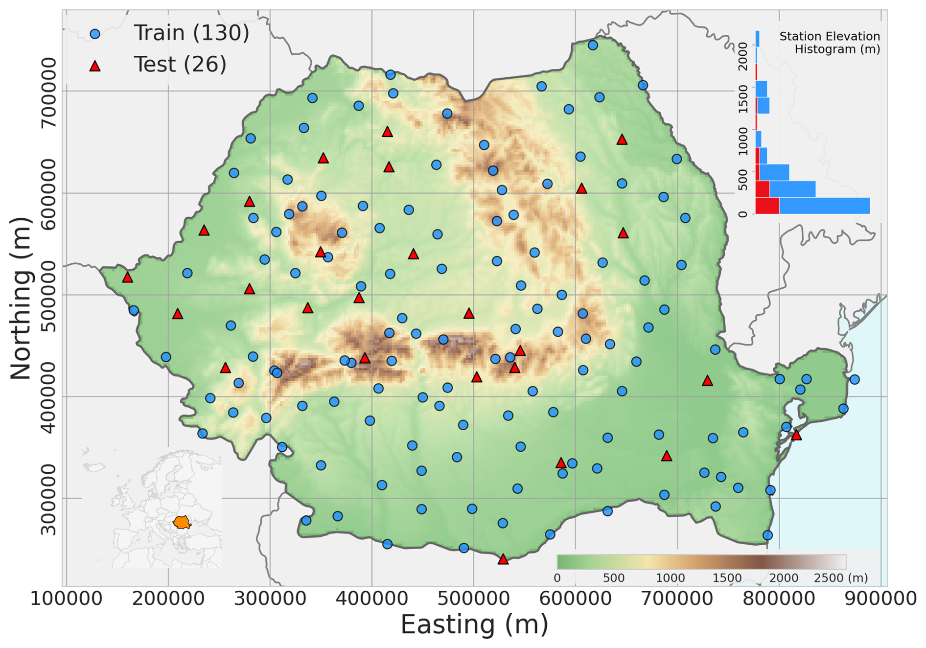
Figure 1 Spatial distribution of the 156 meteorological stations used in this study, overlaid on the SRTM digital elevation model of Romania. Training stations (n=130, blue circles) and held-out test stations (n=26, red triangles) were assigned by random spatial split. The inset histogram shows the elevation distribution of training and test stations, confirming that both subsets span the full altitudinal range of the network (0–2544 m). Coordinates are in the Dealul Piscului 1970 projection (EPSG:31700). Inset map shows Romania's location within Europe. SRTM data © NASA/NGA.

Topographic and geographic predictors are derived from a high-resolution DEM (Jarvis et al., 2008). These predictors serve as covariates in the RK model and as static input features for the DL models. We restricted our input predictors to those derived from topographic data because the primary objective of this study is to identify an interpolation model configuration suitable for application to long-term daily climate time series (1901–present). For this extended historical period, dynamic covariates such as satellite products and land cover datasets are unavailable or inconsistent. Limiting the input to static, topographically derived predictors ensures temporal consistency and model applicability across the full-time span.

2.2 Spatio-temporal covariates

A set of predictor variables was engineered to capture the primary drivers of spatial and temporal climate variability. These are grouped into static spatial predictors and dynamic temporal predictors.

Derived directly from the DEM for every station and grid point location, spatial predictors include smoothed elevation (smooth_elev), a topographic position index (topo_position), distance to the Black Sea (dist_to_coast), and geographic coordinates (latwgs, lonwgs) (Fig. 2) (Daly et al., 2008).

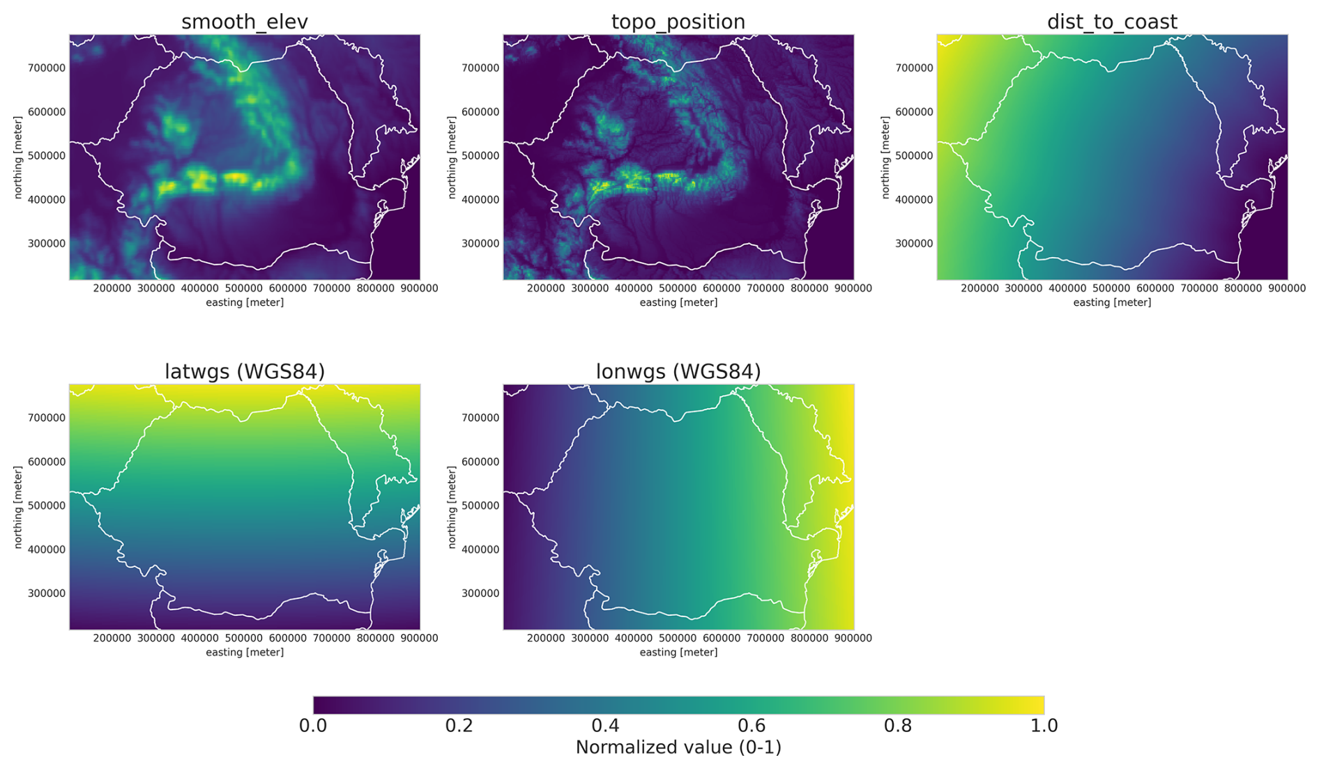
Figure 2 Normalized static predictors used as model inputs (range 0–1): (a) smoothed elevation (smooth_elev), (b) topographic position index (topo_position), (c) distance to the Black Sea coast (dist_to_coast), (d) latitude (latwgs), and (e) longitude (lonwgs). Coordinates are in the Dealul Piscului 1970 projection (EPSG:31700). SRTM data © NASA/NGA.

Calculated for each day to capture seasonal and long-term patterns, temporal predictors represent cyclical patterns without discontinuities, the day of the year and the month are transformed into sine and cosine components (day_sin, day_cos, month_sin, month_cos). A year_scaled variable, representing the year linearly scaled to the [0, 1] range over the analysis period, is included to account for inter-annual trends. These predictors are concatenated to form a feature vector for each observation point (context) and prediction grid point (target).

To assess whether the station network adequately represents the prediction domain, Fig. 3 compares the distributions of the three key static predictors – smoothed elevation, topographic position index, and distance to the Black Sea coast – across training stations, test stations, and the prediction grid (restricted to cells within Romania's national territory). The training and test station distributions are closely aligned across all predictors, confirming that the random $\mathrm{130}/\mathrm{26}$ split is representative. Crucially, the prediction grid falls almost entirely within the training data envelope: only 0.4 % of grid cells exceed the maximum training-station elevation, 0.1 % exceed the maximum topographic position, and 0.5 % exceed the maximum distance to coast. These results indicate that the model operates predominantly within its training distribution during grid-scale prediction, with extrapolation limited to a small number of extreme-topography cells.

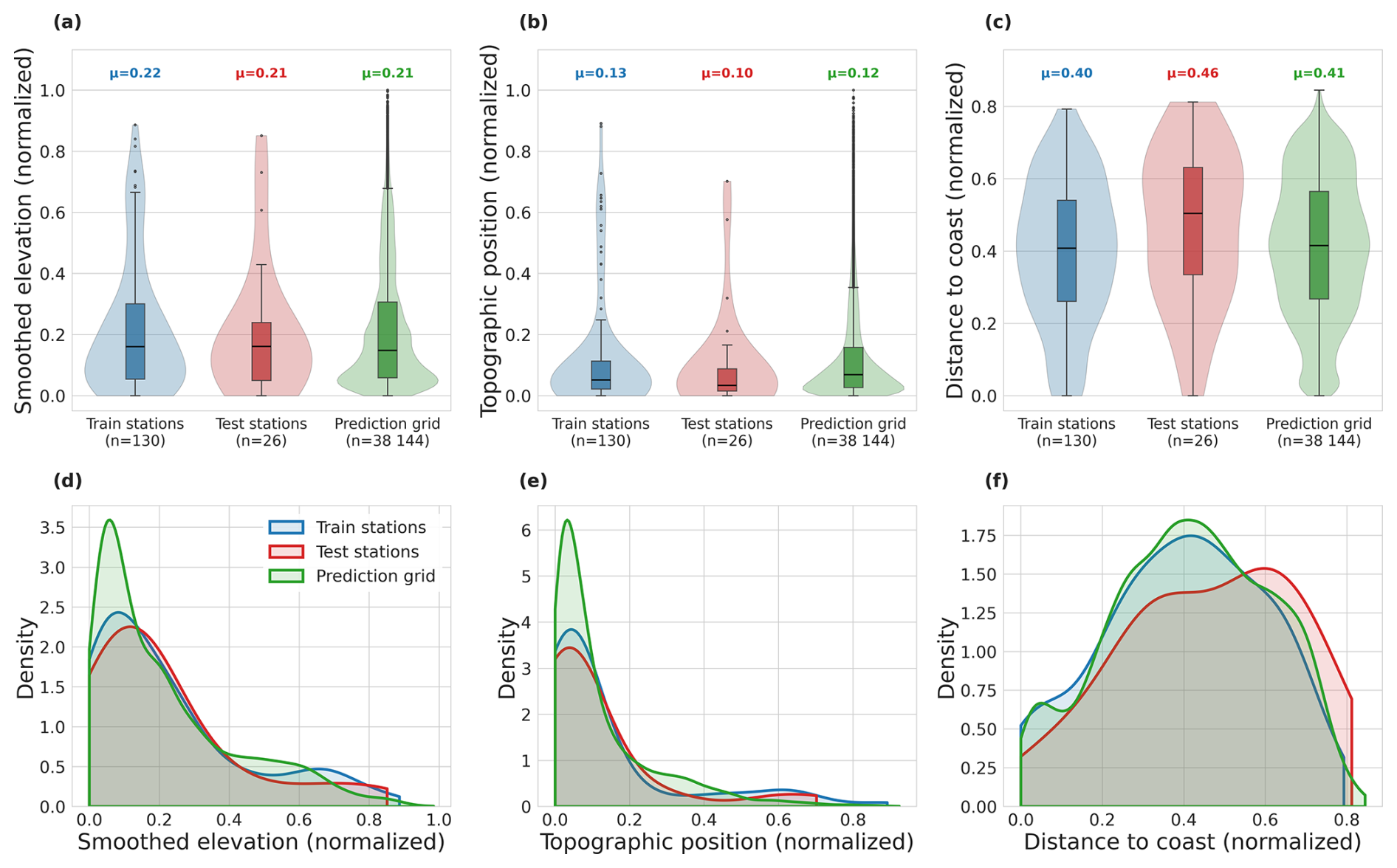
Figure 3 Distribution of key static predictors across training stations (n=130), test stations (n=26), and prediction grid cells within Romania (n=38 144). (a–c) Violin plots with overlaid box plots for smoothed elevation, topographic position index, and distance to the Black Sea coast, respectively; the mean value (μ) for each distribution is indicated at the top of the panels. (d–f) Kernel density estimates for the same three predictors. Predictor values are shown in their normalized [0,1] form.

2.3 Data preprocessing

The raw data are processed into a format suitable for training the deep learning models. This involves normalization of the target variables and structuring the data into daily context and target sets.

The two climate variables, temperature and precipitation, are normalized independently. The daily mean temperature (tavg) is linearly scaled to a [0, 1] range using a Min-Max scaler fitted on the training data (Pedregosa et al., 2011). Raw precipitation (prec) values p are transformed via log(1+p) to handle zero values and reduce skewness, and the transformed values are then scaled to the range [0, 1].

The parameters of these scalers are saved and used to de-normalize the model's predictions back to their original physical units (°C and mm) during validation and inference.

3 Methods

The core of our study is the comparison of a standard approach – the geostatistical method Regression Kriging (RK) – with deep learning architectures, namely the Spatial Multi-Attention Conditional Neural Process (SMACNP). Unlike RK, the deep learning models are used to jointly predict both air temperature and precipitation in a single realisation. The modelling approach differs fundamentally for the two variables due to their distinct statistical characteristics: air temperature, a continuous variable, is modelled directly, whereas daily precipitation, which is intermittent and non-negative, is handled using a two-part hurdle modelling framework in all tested configurations.

3.1 Regression Kriging (RK)

For air temperature, RK is applied directly to observed values. For precipitation, we employ a hurdle framework where occurrence and amount are modelled independently. In both cases, the field is decomposed into a deterministic trend estimated via multiple linear regression on all static and temporal predictor variables (smoothed elevation, topographic position index, distance to coast, geographic coordinates, and cyclic day-of-year/month/year encodings), and a stochastic residual interpolated using Ordinary Kriging with a spherical semi-variogram model. The variogram parameters (partial sill, range, and nugget) are estimated automatically for each daily field via weighted least-squares fitting. The detailed mathematical formulation is provided in Appendix A.

3.2 SMACNP

The Spatial Multi-Attention Conditional Neural Process (SMACNP) is a probabilistic deep learning model designed for interpolating sparse and irregularly distributed spatio-temporal data. It employs an encoder-decoder architecture that maps a set of observed context points to predictive distributions at unobserved target locations.

The model is conditioned on a set of N context points representing observed data. Each context point consists of spatial coordinates (s), a vector of auxiliary attributes (x), and the corresponding climate variable measurement (y). Predictions are made at a set of M target locations, each defined by its spatial coordinates (s^*) and attributes (x^*) (Fig. 4).

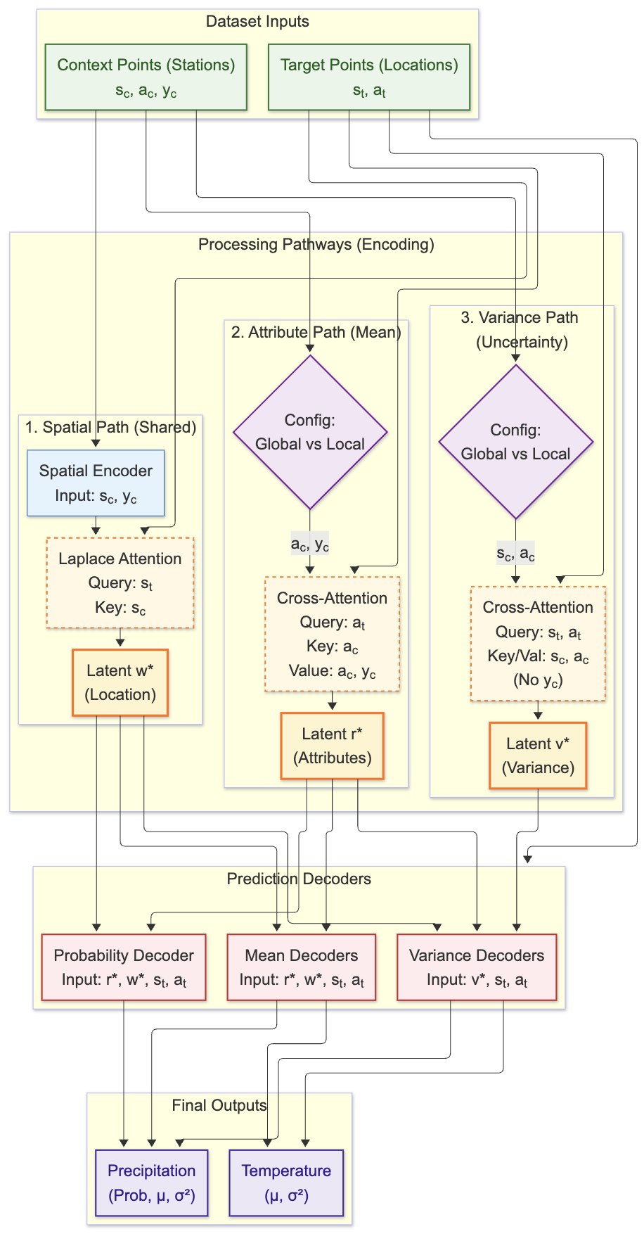
Figure 4 SMACNP architecture with dual encoder configurations. Three encoding pathways produce latent representations: spatial (w^*) via Laplace attention, mean attributes (r^*), and variance (v^*). The mean and variance pathways offer interchangeable configurations: Global  – full N×M attention on attributes only; Localized – k-NN attention on spatial coordinates plus attributes with optional positional encoding. Note that the variance pathway excludes observations (y_c) in both configurations to enable proper uncertainty estimation. Shared MLP decoders output temperature (μ, σ²) and precipitation (probability p, μ, σ²) predictions.

The encoder is composed of three parallel pathways that process the input data into latent representations (Fig. 4):

• i.

  Spatial Pathway (Mean Location Encoder). This pathway captures the spatial structure of the observations. It projects the concatenation of context coordinates and observations through a Multi-Layer Perceptron (MLP – a feedforward neural network applying successive linear transformations with nonlinear activations), then applies Laplace Attention – a distance-based weighting kernel using a configurable L_p norm (p=1 for Manhattan distance, p=2 for Euclidean distance):

  $$\begin{array}{}\text{(1)}& w\left({\mathit{s}}^{*},{\mathit{s}}_i\right)\propto \exp \left(-\mathit{\tau }\cdot \parallel {\mathit{s}}^{*}-{\mathit{s}}_i{\parallel }_p\right)\end{array}$$

  where τ is a learnable temperature parameter. This produces a location-based representation w^* that encodes the spatial structure of the data.

• ii.

  Attribute Pathway (Mean Attribute Encoder). This pathway computes an attribute-based representation r^* using Multi-Head Attention. The mechanism operates through three vectors – Query (Q), Key (K), and Value (V) – that can be understood intuitively in the context of spatial interpolation. The Query encodes what the target location needs: “find stations with similar geographic and seasonal characteristics to mine” (e.g., similar elevation, topographic position, and time of year). The Key encodes what each context station offers: its own geographic and seasonal characteristics, which are compared against the Query to determine relevance. The Value contains the actual information to transfer: the context station's characteristics together with its observed measurements (temperature, precipitation). The attention output is a weighted combination of V, where stations whose Key is most similar to the target's Query receive the highest weights – effectively retrieving weather observations from the most geographically and seasonally relevant stations. The two encoder configurations differ in how Q, K, and V are constructed (Table 1): The Localized configuration restricts attention to the k nearest spatial neighbors, introducing an inductive bias towards spatial locality that is well-suited for meteorological interpolation.

• iii.

  Variance Pathway. This pathway produces a representation v^* for estimating predictive uncertainty. It uses the same attention mechanism as the attribute pathway, but crucially excludes the observations (y) from the Value vectors. This prevents the model from memorizing input-output relationships and enables well-calibrated uncertainty estimates that reflect the information available at each target location.

Table 1 Definition of the query, key, and value inputs used by the Global and Localized SMACNP configurations.

The latent representations are routed to specialized decoder heads, each implemented as an MLP. The spatial and attribute representations (w^*, r^*) are concatenated with target information and fed to the heads predicting mean values and probabilities. The variance representation (v^*) is similarly combined with target information and fed to the variance heads.

The decoder produces parameters for two predictive distributions. Air temperature is represented by a Gaussian distribution parameterized by its mean (μ) and variance (σ²); the mean uses a linear activation, while the variance uses a Softplus activation to ensure positivity. Precipitation is represented by a hurdle model that separates occurrence from amount. A Bernoulli component models precipitation occurrence via logistic activation, while a Gaussian component models the normalized, log-transformed precipitation amount conditional on occurrence. The corresponding variance is constrained to be positive using a Softplus activation.

The model is trained end-to-end by minimizing a combined loss comprising the Gaussian negative log-likelihood (NLL) for temperature, binary cross-entropy for precipitation occurrence, and Gaussian NLL for the normalized, log-transformed precipitation amount on wet days. To address class imbalance between rainy and dry days, the BCE loss incorporates a positive class weight. The full loss equations are provided in Appendix C.

3.3 Experimental setup

Although the source observations can be stored as station-day records, SMACNP does not treat them as independent tabular samples. Each day is represented as a spatial interpolation task consisting of a set of observed context stations and a set of target locations. The training protocol involves two nested levels of data partitioning. First, the available days (2020–2023) are split into 80 % for training and 20 % for validation; the validation set is used exclusively for early stopping and model checkpoint selection. Second, within each training day, the 130 training-pool stations are randomly partitioned into a context set (∼ 50 % of stations, used as model input) and the training loss is evaluated at all 130 stations (“on-the-grid” training). This means the model must learn both to reconstruct observations at context stations and to interpolate at the remaining non-context stations – the latter constituting the genuine test of generalization at each training step. The context partition is re-randomized at every training step, ensuring that every station regularly serves in both roles and that the model learns to interpolate from arbitrary subsets. All data normalization (min–max scaling) is fitted exclusively on the training-pool stations and applied without re-fitting to the test stations at evaluation time. An extensive hyperparameter optimization (HPO) was conducted for the SMACNP model for both global and localized encoder configurations to identify the optimal architecture and training settings. The HPO process was managed using the Optuna framework (Akiba et al., 2019). For each model variant, we executed a total of 1000 trials. The optimization was guided by a Tree-structured Parzen Estimator (TPE) sampler, initialized with a fixed random seed to ensure reproducibility. The objective for each trial was to minimize the model's validation loss. While the learning rate was included in the hyperparameter search space (ranging from $\mathrm{1}\times {\mathrm{10}}^{-\mathrm{5}}$ to $\mathrm{5}\times {\mathrm{10}}^{-\mathrm{4}}$), other training parameters were held constant. We used the AdamW optimizer with a weight decay of $\mathrm{1}\times {\mathrm{10}}^{-\mathrm{5}}$. The learning rate was managed by a scheduler configured to reduce the rate upon plateauing validation loss. To efficiently explore the search space, we implemented an aggressive early-stopping strategy, training each trial for up to 1500 epochs. A patient pruner (wrapping a median pruner) was configured to terminate unpromising trials. Trials were pruned if their validation loss exceeded the median of previously completed trials for consecutive checks (patience of 5 checks), performed every 10 epochs after an initial warmup period (150 epochs).

The search spaces for the two configurations, including embedding dimensions, attention heads, and learning rates, are detailed in Appendix B. A constraint was enforced to ensure that embedding dimensions (r_dim, v_dim) were divisible by the number of attention heads.

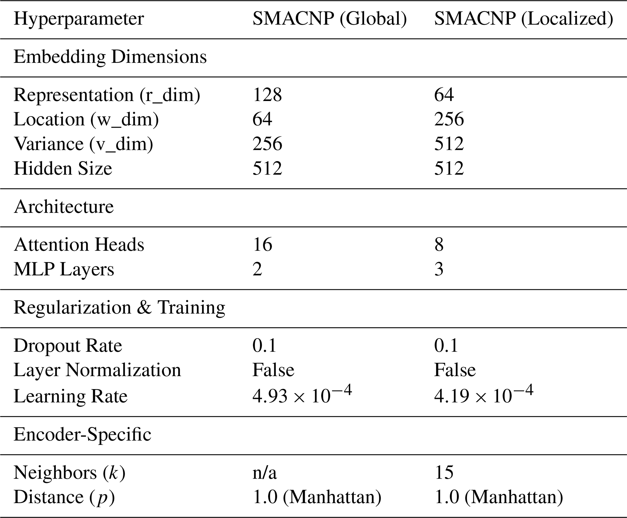
Following the optimization process, the configurations yielding the lowest validation loss were selected for the final training and evaluation (Table B1). The SMACNP (Global) configuration favoured a balanced architecture with a representation dimension (r_dim) of 128 and a variance dimension (v_dim) of 256. It utilized a shallower decoder (2 MLP layers) and higher attention complexity (16 heads) with minimal regularization (dropout rate of 0.1 and no layer normalization).

The SMACNP (Localized) configuration achieved optimal performance with a neighbourhood size k=15 and, like the global variant, utilized the Manhattan distance metric (p=1) for the Laplace attention. The architecture favored a highly asymmetric embedding structure, allocating significant capacity to the variance (v_dim=512) and location (w_dim=256) pathways while keeping the representation dimension compact (r_dim=64). The decoder was deeper than the global variant (3 vs. 2 MLP layers), but the optimization selected the same lightweight regularization – dropout rate of 0.1 and no Layer Normalization – suggesting that the inductive bias of localized attention provides sufficient regularization on its own. Both models converged to similar learning rates ($\mathrm{4.93}\times {\mathrm{10}}^{-\mathrm{4}}$ for the global variant, $\mathrm{4.19}\times {\mathrm{10}}^{-\mathrm{4}}$ for the localized one).

4 Results

We evaluated the results both qualitatively, by plotting multiannual-mean maps to verify that the predictions follow the expected spatial distribution of the analysed variables, and quantitatively, by computing accuracy metrics and corresponding plots using independent station data withheld from the training and prediction processes.

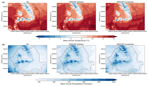
Visually, the outputs for air temperature from the three models are remarkably consistent (Fig. 5a), showing nearly identical spatial distributions, successfully capturing the expected climatological patterns driven by the topography. All methods correctly identify the same locations for the coldest areas in the mountain ranges and the warmest areas in the lowlands, displaying comparable temperature gradients. This suggests that the deep learning models are fully capable of reproducing the dominant geographical factors influencing temperature distribution as effectively as the geostatistical baseline. Similar to the temperature results, all three models successfully represent the fundamental influence of topography on precipitation (Fig. 5b). However, the visual differences in spatial detail are much more pronounced here.

The SMACNP Localized precipitation fields exhibit finer spatial detail than RK, particularly over the Carpathian arc where orographic gradients are steepest. Whether this additional detail reflects genuine skill in resolving local precipitation patterns or spatial artefacts would require validation against independent high-resolution observations (e.g., radar composites or dense temporary networks), which is beyond the scope of this study.

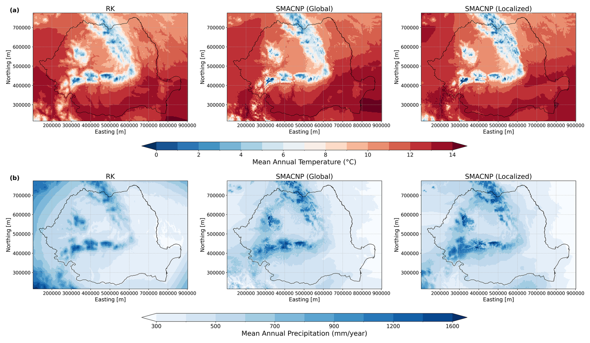
Figure 5 Comparison of predicted mean annual temperature (a) and precipitation (b) from three models: RK, SMACNP (Global), and SMACNP (Localized).

The density scatter plots in Fig. 6 demonstrate that all three models provide highly accurate predictions for daily mean temperature (panel a), with points clustering tightly along the 1:1 line of perfect agreement. The RK baseline achieves a correlation of 0.989 but exhibits slightly larger dispersion around the 1:1 line compared to the deep learning models, resulting in a higher MAE (0.938 °C). Both deep learning configurations outperform the baseline, with the SMACNP (Localized) variant achieving the best overall performance (MAE = 0.803 °C, RMSE = 1.108 °C), surpassing the SMACNP (Global) configuration (MAE = 0.838 °C). Across all models, prediction errors are slightly more pronounced in the tails of the distribution, yet the high density of points near the diagonal indicates strong agreement across the majority of the temperature range.

In contrast, the performance gap between the methods is more distinct for daily precipitation (panel b). Both SMACNP configurations substantially outperform the RK baseline, which suffers from larger errors (MAE = 1.181 mm) and a lower correlation (0.692). The SMACNP (Localized) model again delivers the strongest performance, achieving the lowest MAE (1.050 mm) and a correlation of 0.749, representing a notable improvement over the geostatistical baseline. While all models struggle with extreme precipitation events – a common challenge in climatological modelling – the deep learning approaches demonstrate a superior ability to capture the variability of moderate-to-high rainfall events compared to RK.

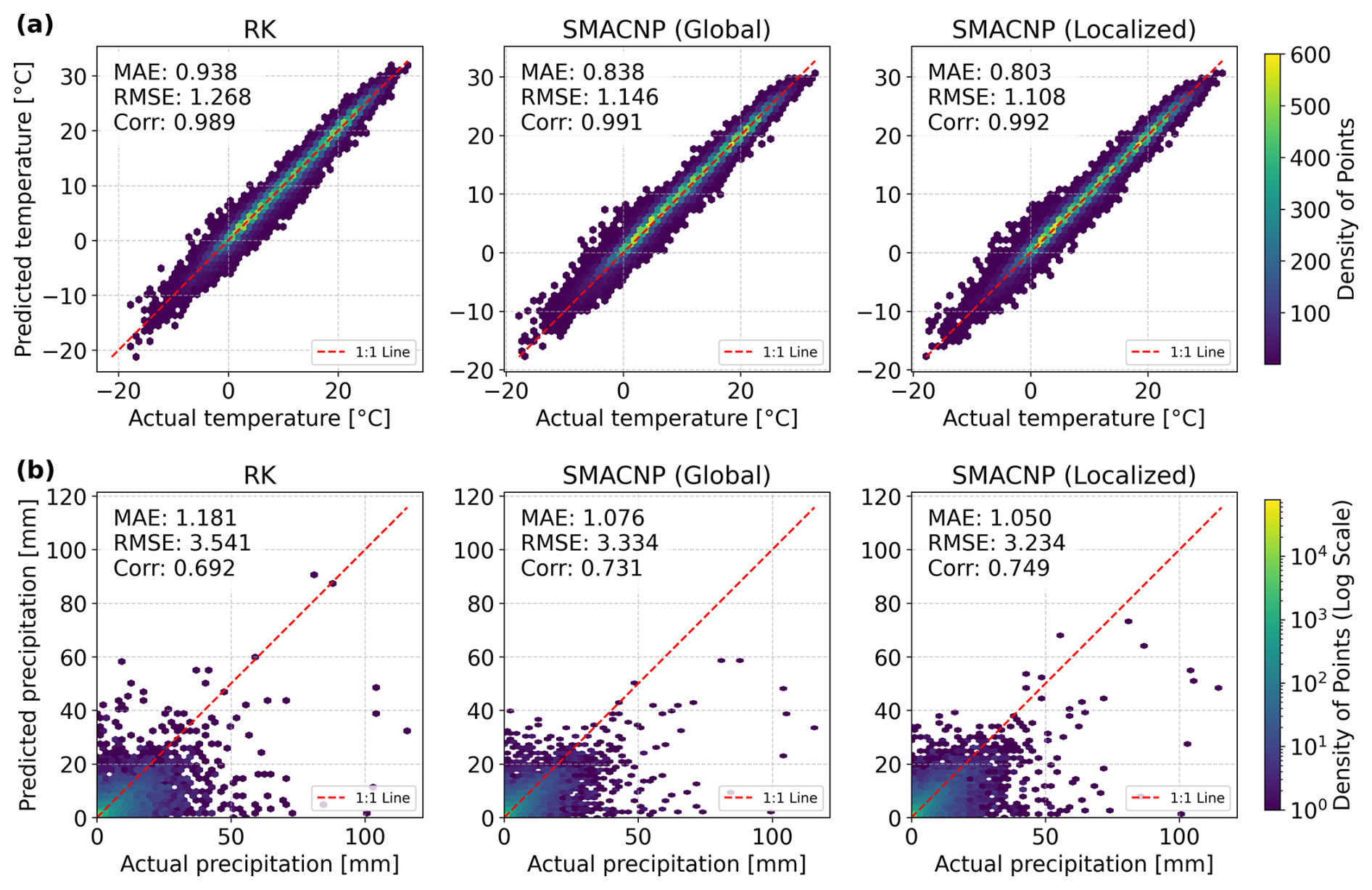
Figure 6 Density scatter plots of predicted versus actual (a) daily mean temperature (°C) and (b) daily precipitation (mm) for the three models on the test dataset: RK, SMACNP (Global), and SMACNP (Localized). For temperature, the colour of each hexagonal bin indicates point density on a linear scale, while for precipitation (zero-inflated data), density is shown on a logarithmic scale. The dashed red line represents the 1:1 line of perfect agreement.

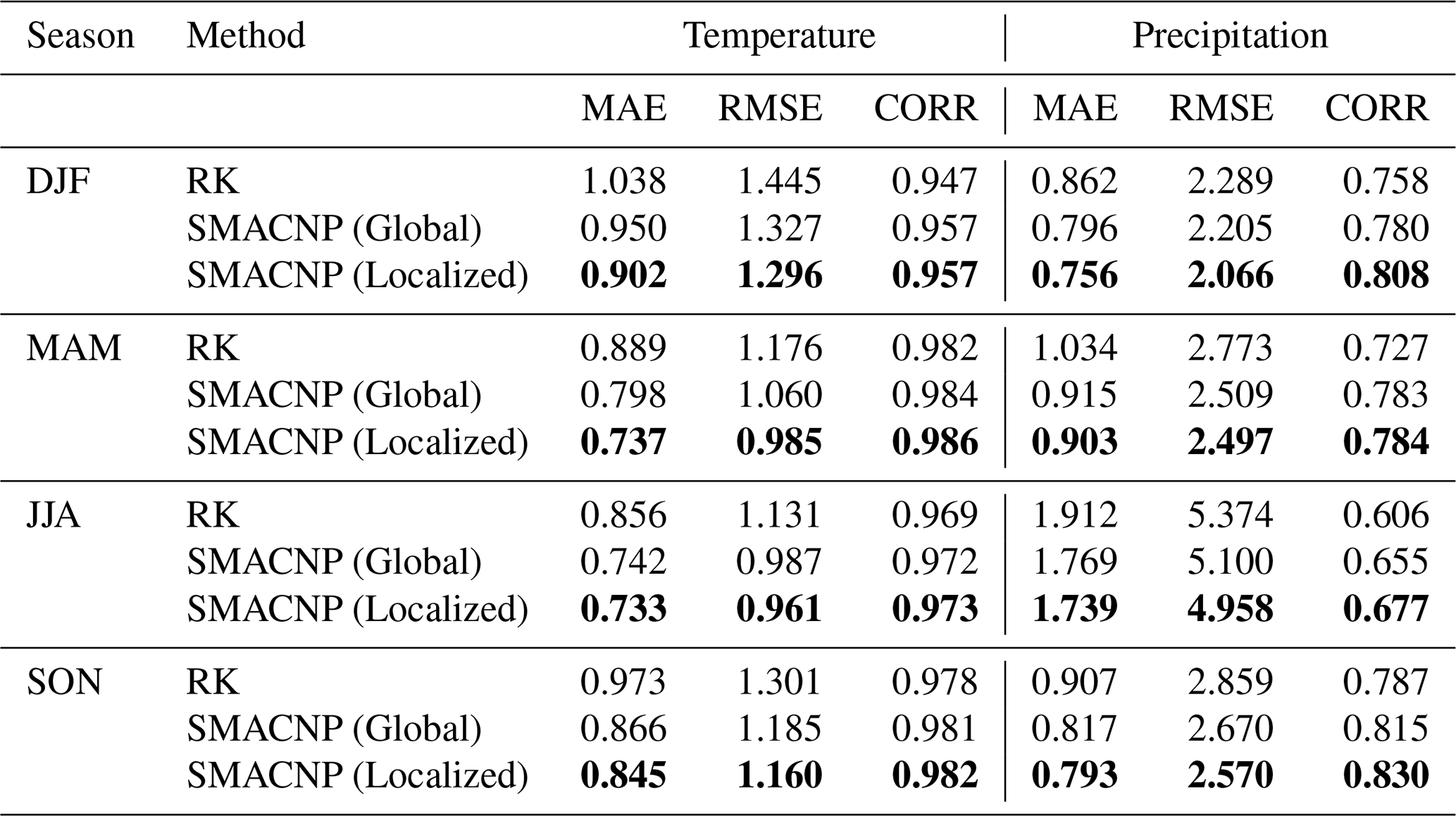
Across all seasons, SMACNP (Localized) and SMACNP (Global) consistently outperform the RK model for both precipitation and temperature (Table 2).  For temperature, all models perform well, with correlations exceeding 0.94 in all cases. SMACNP (Localized) surpasses the others across all four seasons, consistently achieving the lowest MAE and RMSE, reflecting its superior advantage in capturing fine-scale temperature variations compared to both the Global variant and the RK baseline. For precipitation, SMACNP (Localized) demonstrates dominant performance, achieving the lowest MAE and RMSE across all seasons, as well as the highest correlations (e.g., 0.808 in DJF). While SMACNP (Global) remains competitive, SMACNP (Localized) outperforms it even in summer (JJA), yielding the lowest RMSE (4.958) and highest correlation (0.677). The RK model exhibits the weakest performance, particularly for precipitation during JJA, where RMSE reaches 5.374. Overall, the results demonstrate that neural process–based models substantially enhance predictive accuracy over the baseline RK approach, especially for precipitation, where spatial heterogeneity and nonlinearity are more pronounced. Based on its superior performance across the majority of metrics – particularly MAE – and seasons, SMACNP (Localized) emerges as the most consistently high-performing method overall.

Table 2 Seasonal evaluation metrics for temperature and precipitation across all models. Bold values indicate the best-performing model for each metric and season.

To validate the choice of SMACNP over alternative neural process architectures, we also evaluated ConvCNP (Gordon et al., 2019) and GriddedTNP (Ashman et al., 2024), two grid-based models that discretize station observations onto a regular grid before processing with a convolutional backbone. For temperature, neither grid-based architecture matched SMACNP Localized: GriddedTNP achieved an MAE of 1.05 °C – approaching Regression Kriging (0.94 °C) – while ConvCNP yielded 1.53 °C. For precipitation, both models performed competitively, with ConvCNP (MAE = 1.11 mm) approaching SMACNP Localized (1.05 mm) and GriddedTNP (1.22 mm) approaching RK (1.18 mm). The asymmetric performance across variables reflects a fundamental architectural trade-off: grid discretization preserves the large-scale spatial patterns that drive precipitation but smooths the fine-scale topographic contrasts critical for resolving temperature lapse rates in complex terrain. SMACNP's station-to-station attention mechanism avoids this information loss, explaining its consistent superiority across both variables.

To complement the error analysis, we further examine how well the models quantify uncertainty and represent the full precipitation distribution (Fig. 7 and Table 3). For temperature (panel a), the z-score distributions show mean values generally close to zero (Table 3; $\left|\mathrm{mean}z\right|\le \mathrm{0.14}$), though SMACNP (Global) shows a slight positive bias (+0.14). The RK baseline exhibits a narrow z-score distribution (SD ≈ 0.70) resulting in conservative, over-dispersive 95 % intervals (95 % coverage ≈ 0.99). SMACNP (Global) approaches a standard normal distribution (SD ≈ 0.99) with slightly under-dispersive coverage (93.7 %), while SMACNP (Localized) maintains a standard deviation of ≈ 0.87 and achieves coverage closest to nominal (1σ: 0.81, 95 %: 0.96). These improvements are reflected in the temperature CRPS, where both SMACNP configurations outperform RK (0.59–0.62 vs 0.72, with a slight advantage for the localized model). For precipitation amounts on wet days (panel b), all models exhibit negative mean z-scores, indicating a systematic underestimation of the intensity of rainy events. This bias is strongest for RK (mean $z\approx -$0.70) and reduced for the SMACNP variants ($\approx -$0.46 to −0.47). The spread of z-scores is much larger than one for all models, reflecting the strong skewness and heavy tails of the wet-day distribution, but again the deep models show substantial gains: the standard deviation drops from ≈ 3.15 (RK) to 2.73 (SMACNP Global) and 1.92 (SMACNP Localized). The 95 % coverage on wet days increases from 0.90 for RK to about 0.93 for both SMACNP variants, indicating that extreme wet events are captured more reliably, though some under-dispersion remains. Consistently, the CRPS for wet-day precipitation decreases from 2.30 (RK) to 2.13 and 2.12 for the global and localized SMACNP models, respectively. Panel (c) focuses on precipitation occurrence, implicitly derived from the marginal predictive distributions. All models maintain high hit rates for rainy days (≈ 0.95–0.96), but they differ notably in how often they falsely predict rain. RK strongly overestimates the frequency of wet days (predicted wet fraction ≈ 0.57 vs observed ≈ 0.34), leading to a high false-alarm rate of about 0.38 and a relatively low correct-dry rate of 0.63. Both SMACNP configurations bring the predicted wet fraction much closer to the observed value (≈ 0.47–0.48), reduce the false-alarm rate to about 0.23, and increase the correct-dry rate to ≈ 0.77. This indicates fewer spurious light-rain estimates while preserving sensitivity to true rain events. The coverage summary in panel (d) integrates these results. For temperature, RK over-covers at the 95 % level (0.99), whereas SMACNP (Global) slightly under-covers (0.94) and SMACNP (Localized) is near-ideal (0.96). For wet-day precipitation, the RK intervals are too narrow in the tails (95 % coverage ≈ 0.90), while SMACNP models increase the 95 % coverage to ≈ 0.93 and modestly over-cover at 1σ (0.84), consistent with somewhat wider but more reliable uncertainty intervals. Finally, the CRPS scores in panel (e) summarise overall probabilistic skill in a distribution-agnostic way. For both temperature and precipitation (all days and wet days only), the two SMACNP variants consistently achieve lower CRPS than RK, with the localized version marginally outperforming the global one. Taken together, these diagnostics show that the deep learning approaches, and particularly SMACNP (Localized), not only reduce deterministic errors but also provide better-calibrated and more informative uncertainty estimates, especially for precipitation occurrence and intensity.

To further characterize precipitation performance, we computed seven climate-relevant diagnostics at the held-out test stations (Table 4). Wet-day frequency bias is the ratio of predicted to observed wet-day counts (threshold ≥ 1.0 mm, WMO standard), where 1.0 indicates unbiased frequency. Mean intensity bias is the ratio of mean predicted to mean observed precipitation on wet days, capturing whether the model systematically under or overestimates rainfall amounts. Wet-day MAE and wet-day RMSE measure the average absolute and root-mean-square errors, respectively, computed only on observed wet days. R95p bias and R99p bias are the percentage deviations in total precipitation from days exceeding the 95th and 99th percentiles of the observed wet-day distribution, respectively, computed per station per year following the ETCCDI standard (Klein Tank et al., 2009) and then averaged across all station-years. Rx1day bias is the percentage deviation in the mean annual maximum one-day precipitation, computed per station per year following the same standard. All models slightly overpredict wet-day frequency (∼ 20 % overestimation) and underestimate wet-day intensity, consistent with the smoothing inherent in spatial prediction methods. SMACNP Localized shows the smallest biases across all diagnostics, including frequency (1.193), intensity (0.762), aggregate extreme indices (R95p bias: −51 %; R99p bias: −61 %), and Rx1day (−27 %). The underestimation of extreme precipitation totals is a known limitation of spatial interpolation from sparse networks, where individual convective events may not be captured by the nearest context stations.

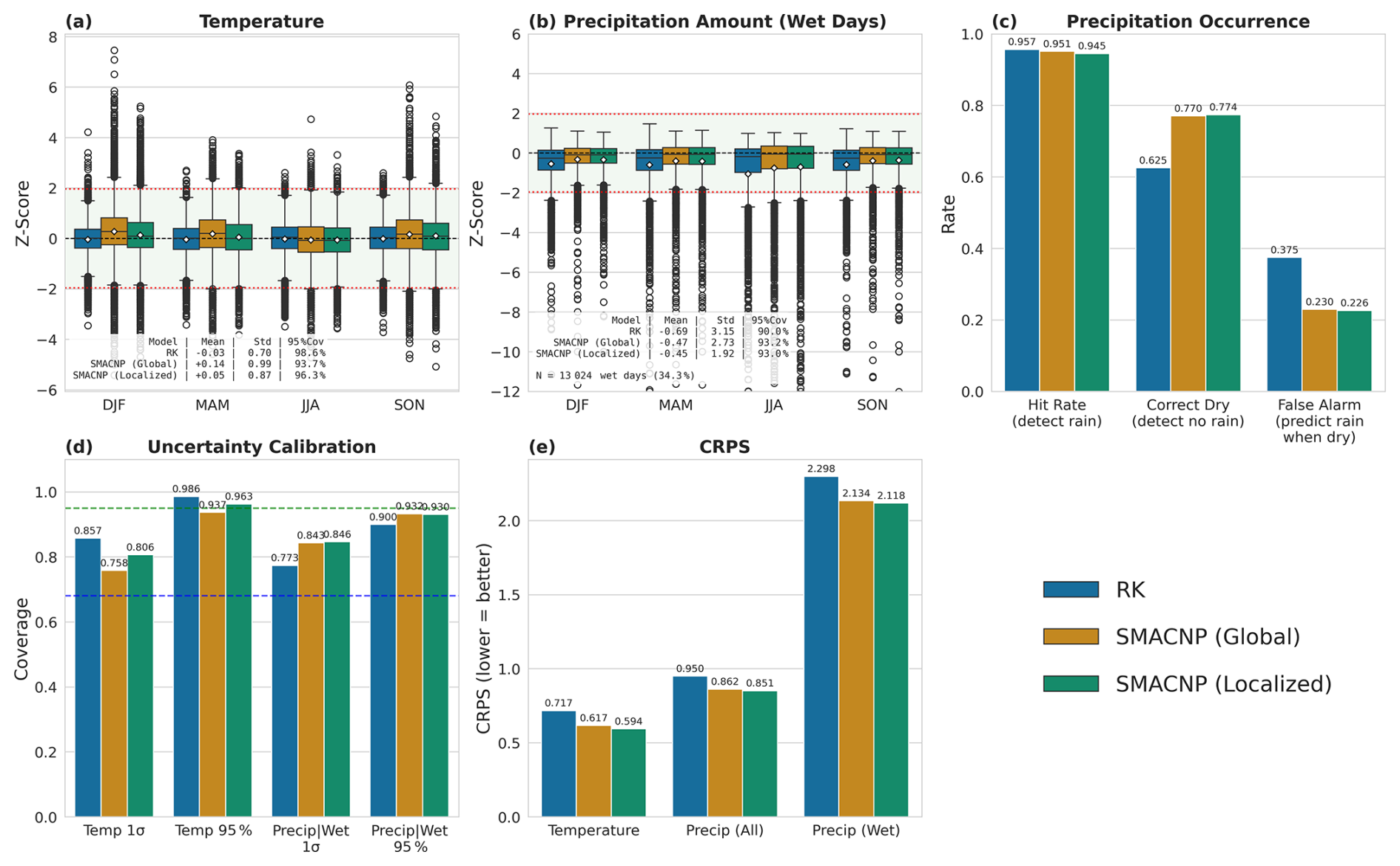
Figure 7 Seasonal uncertainty calibration and overall probabilistic verification. (a) Seasonal distributions of standardized errors (z-scores) for temperature. (b) As in (a), but for precipitation amounts on wet days only (observed precipitation > 0.1 mm; sample size and wet-day fraction indicated in the panel). Z-scores are defined as (prediction − observation)$/$predicted_std; the red horizontal lines mark ±1.96, corresponding to the 95 % interval of a standard normal distribution and used as a visual reference for well-calibrated predictions (mean ≈ 0, SD ≈ 1). (c) Precipitation occurrence scores implicitly derived from the marginal predictive distributions: hit rate for rain detection, correct-dry rate, and false-alarm rate (predicting rain when it is dry). (d) Empirical coverage of the nominal 1σ and 95 % predictive intervals for temperature and precipitation (wet days), with dashed horizontal lines indicating the expected values of 0.68 and 0.95. (e) Continuous Ranked Probability Score (CRPS) for temperature, all-day precipitation, and wet-day precipitation (lower values indicate better probabilistic skill).

Table 3 Summary of probabilistic verification metrics for temperature and precipitation. Metrics are aggregated over all seasons and stations for the three methods (RK, SMACNP Global, SMACNP Localized). For temperature, CRPS quantifies overall probabilistic skill (lower is better), “95 % Cov” is the empirical coverage of the nominal 95 % predictive interval, and “Mean Z” is the mean standardized error, with an ideal value of 0. For precipitation detection, scores are computed using an occurrence threshold of 0.1 mm: Hit Rate is the fraction of wet days correctly detected, FAR (false alarm rate) is the fraction of dry days on which rain is predicted, and True Dry is the fraction of dry days correctly forecast as dry. For precipitation intensity, CRPS, 95 % coverage and Mean Z are evaluated on wet days only (observed precipitation > 0.1 mm). An ideal model has low CRPS and FAR, high Hit Rate and True Dry, 95 % Cov close to 0.95, and $\left|\mathrm{Mean}Z\right|$ close to zero. Bold values indicate the best-performing model for each metric.

Table 4 Climate-relevant precipitation diagnostics at held-out test stations (n=26), 2020–2023. Wet-day threshold =1.0 mm (WMO standard). Frequency and intensity biases are expressed as ratios (1.0= unbiased). R95p, R99p, and Rx1day biases are expressed as percentage deviations from observed values. Bold values indicate the best (closest to unbiased) performance for each diagnostic.

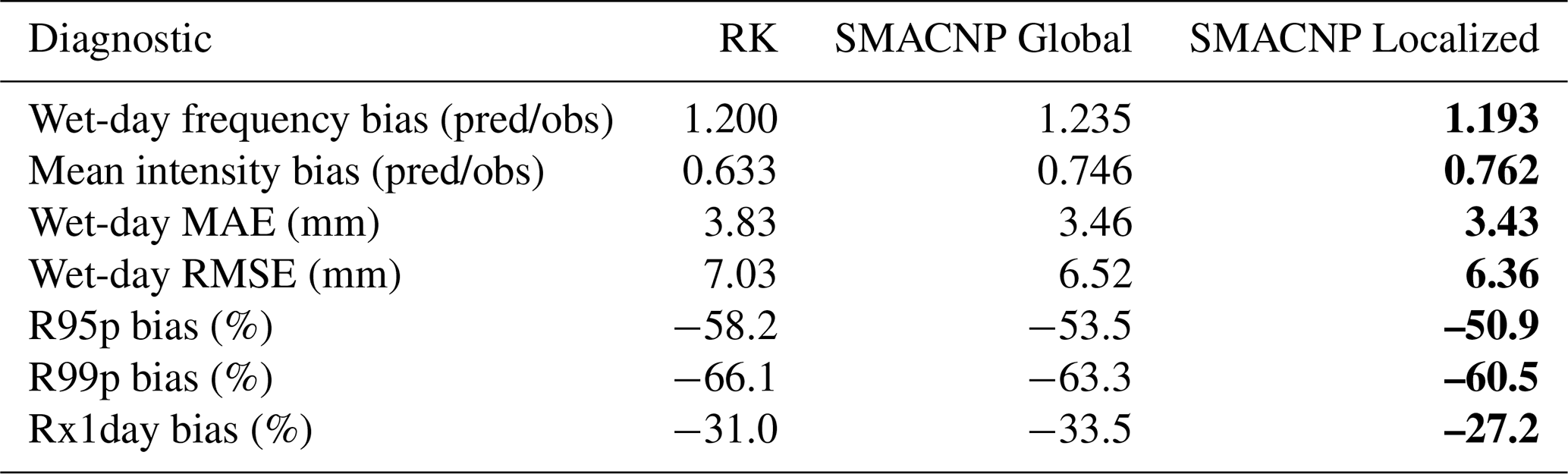
Figure 8 provides a time-series comparison of model performance for daily mean air temperature and total precipitation at the Bacău station (174 m a.m.s.l.) throughout 2023, selected from the test data subset. The figure shows the ground truth observations against the predictions from the three evaluated models.

For air temperature, all three models demonstrate a strong ability to capture the seasonal cycle and daily fluctuations, closely tracking the ground truth data. The shaded areas, representing the 95 % predictive intervals, are relatively narrow for all models, indicating a high degree of certainty in their temperature predictions, though the RK intervals are noticeably wider than those of the deep learning models. The MAE values inset in the plot show that the deep learning models outperform the baseline, with SMACNP (Localized) achieving the lowest MAE of 0.468 °C, followed by SMACNP (Global) at 0.488 °C, both improving upon the RK model's MAE of 0.575 °C.

The lower panel, illustrating total precipitation, reveals the challenges in modelling this discontinuous variable. While all models capture the timing of major precipitation events, the SMACNP (Localized) model demonstrates the best performance in predicting the magnitude of these events, as evidenced by its lower MAE of 0.663 mm. SMACNP (Global) follows closely with an MAE of 0.687 mm, while the RK model has the highest MAE at 0.789 mm. The 95 % predictive intervals are visibly wider for precipitation than for temperature across all models, reflecting the greater inherent uncertainty in predicting this variable. Notably, the predictive intervals for the deep learning models, particularly SMACNP (Localized), often envelop the observed precipitation peaks more effectively than the RK model, suggesting a more reliable quantification of uncertainty. This is especially apparent during the intense precipitation events observed in September and November.

Corresponding time-series comparisons for all other stations in the test set are provided in the Supplement (Figs. S1–S25), demonstrating consistent performance across diverse elevations and locations.

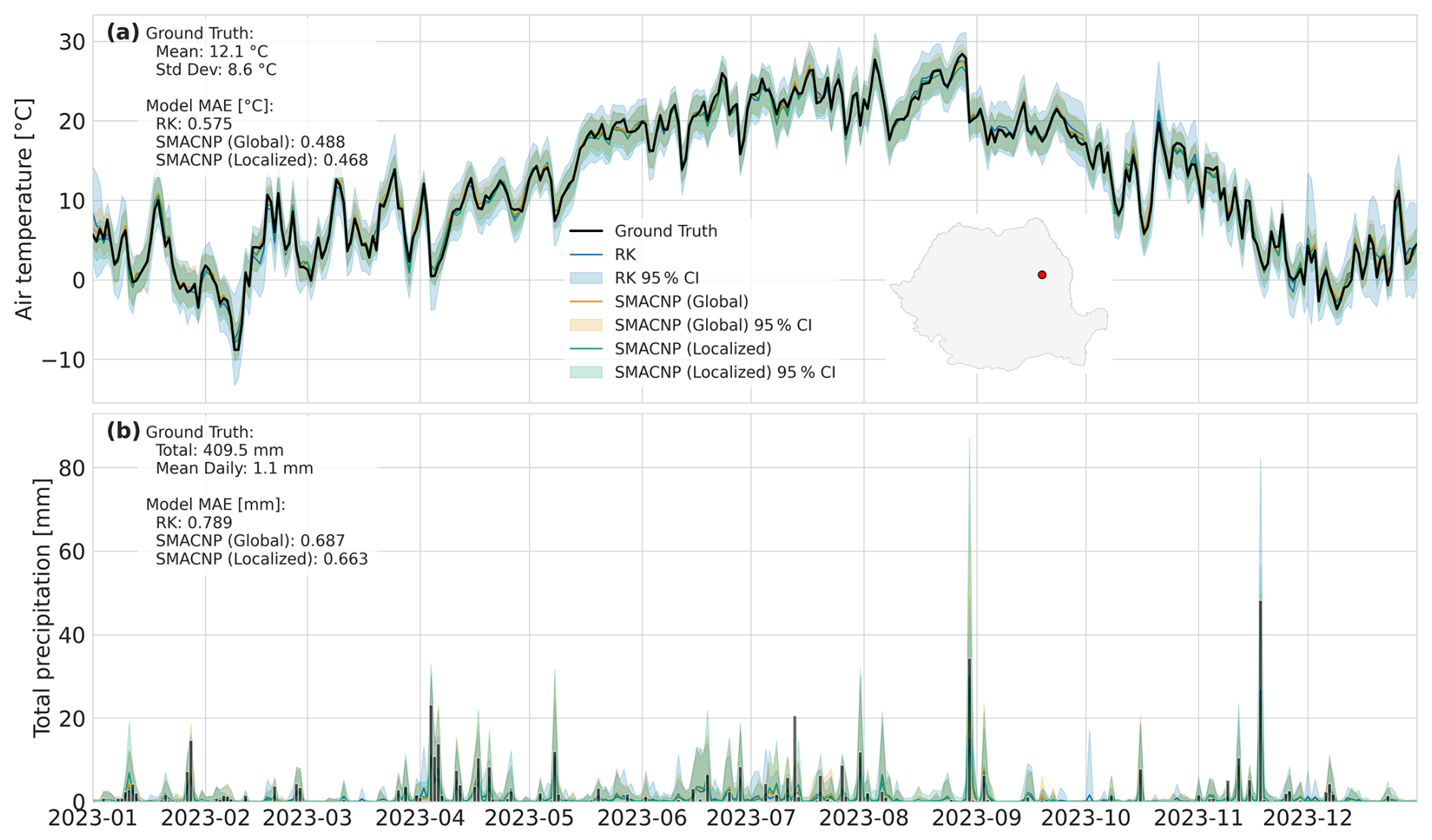
Figure 8 Model performance and uncertainty at Bacău station (174 m a.m.s.l.). Time series comparison of (a) daily average temperature and (b) daily total precipitation for the year 2023. Shaded areas represent the 95 % predictive interval for each model's prediction. The inset map shows the location of the station within the study area, marked by a red dot.

5 Discussion

This study evaluated the SMACNP architecture – an attentive Conditional Neural Process originally proposed for general meta-learning tasks – as a practical alternative to Regression Kriging for daily climate gridding from a sparse national station network over complex terrain. The superior performance of the neural process models, particularly for precipitation, can be attributed to their ability to learn complex, non-linear relationships directly from the data. Unlike RK, which relies on a pre-defined linear model for the trend and a stationary variogram for the residuals, deep learning architectures can capture the intricate interplay between topography, location, and climate variables. This is especially critical for precipitation, whose spatial distribution in mountainous terrain is often intermittent, highly localized, and non-stationary conditions that violate the core assumptions of RK and explain its tendency to produce overly smooth and generalized outputs.

Among the two deep learning architectures, the good results of the SMACNP with a localized encoder highlights the benefit of incorporating a strong structural prior into the model design. This approach aligns with the principles driving recent breakthroughs in global weather forecasting, where models like Google's GraphCast and ECMWF AIFS have demonstrated the importance of effectively capturing local spatial dependencies (Lam et al., 2023; Moldovan et al., 2025). In our application, by restricting the attention mechanism to a k-NN, the localized encoder is explicitly guided to learn representations based on spatial proximity. This provides a powerful inductive bias for modeling climate variables, contrasting with the more flexible, but less constrained, global attention mechanism of the standard SMACNP. Moreover, the localized configuration offers superior computational efficiency when generating high-resolution grids. By limiting interactions to the k nearest neighbours (k-NN) rather than computing global pairwise correlations, it avoids the quadratic complexity of the global encoder, making it significantly more scalable for producing dense gridded outputs. Building on this, future studies could further enhance the configuration by incorporating explicit graph structures within the encoder. Adopting Graph Neural Network (GNN) architectures would allow for sophisticated message passing between observation points, potentially capturing complex, non-linear spatial dependencies more effectively than the current attention-based neighbourhood aggregation.

The practical importance of well-calibrated uncertainty cannot be overstated. For applications such as flood risk assessment or agricultural modelling, an unbiased estimate of the prediction's confidence is as valuable as the prediction itself. Our analysis reveals that only SMACNP (Localized) provides reliable uncertainty estimates across both temperature and precipitation. The severe overconfidence of the RK model's precipitation uncertainties renders them impractical for risk-aware decision-making. Furthermore, the uncertainty quantification of the deep learning models could be enhanced by adopting a deep ensemble approach. As demonstrated in the creation of a global canopy height map from satellite imagery (Lang et al., 2023), training an ensemble of models with different random initializations offers a robust approach to estimate epistemic uncertainty – the model's lack of knowledge in regions or conditions underrepresented in the training data. The variation among ensemble predictions provides a direct measure of model confidence. While the inherent probabilistic design of our SMACNP (Localized) already captures aleatoric uncertainty, combining it with an ensemble strategy would yield a more comprehensive and reliable characterization of total predictive uncertainty, further supporting the adoption of such frameworks for operational climate datasets.

Remarkably, the SMACNP models achieved superior accuracy compared to the RK baseline, even though it was constrained to model temperature and precipitation simultaneously. While RK had the advantage of fitting distinct models for each variable, the deep learning approach demonstrated that a unified architecture could leverage shared spatio-temporal features to outperform the specialized, single-variable geostatistical models.

An advantage of the multivariate SMACNP framework is its ability to learn shared latent representations across climate variables. Because temperature and precipitation are predicted jointly through shared encoder pathways, the model can implicitly capture cross-variable dependencies, for instance, the coupled effects of topography on temperature lapse rates and orographic precipitation enhancement. In classical geostatistics, such dependencies can be exploited through co-kriging, which models cross-variograms between variables. The deep learning approach achieves a similar effect but extends to nonlinear relationships and scales naturally to additional variables (e.g., wind speed, humidity) through additional output heads, without requiring separate models or the estimation of additional cross-variogram parameters. While we do not present a formal univariate ablation in this study, we note that training separate single-variable models is straightforward within the SMACNP framework, and such a comparison would help quantify the benefit of joint variable learning for climate gridding.

The SMACNP model is designed for temporal transferability. Because the model is conditioned on actual station observations at each prediction step, it learns a spatial interpolation function that is largely independent of the specific training period. The topography-climate relationships captured by the encoder are expected to remain valid for periods outside the 2020–2023 training window, provided that the station network density and the underlying spatial structure of the climate fields do not change substantially. Extending the training period to include additional years would improve the model's exposure to rare events and extreme values, and is a priority for future development.

It is also pertinent to address the architectural selection for this study. During the initial phases, we evaluated other neural process variants, including the ConvCNP and GriddedTNP. However, these models failed to yield satisfactory results under the strict constraints of our experimental setup; the combination of a very sparse observation network (130 stations) and the exclusion of dynamic covariates appeared to hinder the ability of these architectures to resolve local features effectively. While GriddedTNP is designed to scale efficiently to large datasets, it likely struggled to construct a robust latent grid representation from such sparse inputs. The SMACNP architecture proved suited to this data-scarce regime because its attention mechanism explicitly models directly the relationship between specific context and target points based on topographic similarity, rather than relying on grid-based projections or convolutions that typically require denser data to perform optimally.

It is important to acknowledge the limitations of this study. Our analysis was intentionally restricted to static, topographically-derived predictors to ensure the developed models are applicable to long-term historical datasets where dynamic covariates like satellite imagery products are unavailable. The inclusion of dynamic predictors could further enhance model performance for modern periods. Also, the evaluation is restricted to a single country. Although Romania presents a demanding combination of topographic complexity, station sparsity, and mixed precipitation regimes, the generalizability of the results to other climatic regions and station network configurations remains to be demonstrated. In particular, the relative advantage of the localized attention mechanism may depend on factors such as station density, the dominant spatial scales of variability, and the degree of topographic control on the target variables. Extending the framework to additional countries or continental-scale networks, and assessing its performance under different data availability conditions, is a priority for future work. A more extensive comparison with alternative nonlinear machine-learning and hybrid machine-learning–geostatistical methods would be useful in future work, particularly if both point-wise accuracy and spatial characteristics of the resulting grids are evaluated.

6 Conclusions

In this study, we evaluated and compared a traditional geostatistical interpolation method, Regression Kriging (RK), with two advanced deep learning models, the Spatial Multi-Attention Conditional Neural Process (SMACNP) with Localized and Global encoders, for producing daily gridded fields of air temperature and precipitation from a very sparse station network in Romania.

The primary conclusions of this work are as follows:

1. Deep learning models substantially outperform the geostatistical baseline. Both SMACNP configurations demonstrated significantly higher accuracy than RK for both climate variables. The performance gains were particularly large for precipitation, where the neural process models were better able to capture the complex, non-linear, and heterogeneous spatial patterns inherent to rainfall in a topographically diverse region.

2. SMACNP (Localized) is the most robust and highest-performing model. Our study identifies this specific configuration as a novel and highly effective approach for sparse data interpolation.  By explicitly leveraging local neighbourhood structure via a localized encoder, the SMACNP (Localized) model consistently achieved the best or near-best performance across most evaluation metrics and seasons. It excelled at creating detailed and realistic spatial fields while minimizing prediction errors.

3. Probabilistic deep learning provides superior uncertainty quantification. A key advantage of the neural process framework is its native ability to provide probabilistic predictions. The SMACNP (Localized) model, in particular, produced well-calibrated and reliable uncertainty estimates for both temperature and precipitation. In contrast, the RK model's precipitation uncertainty estimates showed signs of overconfidence, reducing their reliability.

Our findings demonstrate that a unified deep learning framework can outperform specialized univariate geostatistical models, effectively leveraging shared spatio-temporal patterns to improve accuracy across multiple climate variables simultaneously. The ability of these models to learn from data to represent complex spatial dependencies, combined with their capacity for reliable uncertainty estimation, makes them exceptionally well-suited for the development of high-quality gridded climate datasets. The results of this study provide a strong methodological foundation for the future production of a new, long-term, high-resolution daily climate dataset.

Appendix A: Regression Kriging Formulation

The temperature Z at a location s is modeled as the sum of a deterministic trend m(s) and a stochastic, spatially correlated residual R(s):

$$\begin{array}{}\text{(A1)}& Z\left(s\right)=m\left(s\right)+R\left(s\right)\end{array}$$

The prediction $\widehat{Z}\left(s_{\mathrm{0}}\right)$ at a target location s₀ is derived in three steps:

1. The trend m(s) is estimated using a multiple linear regression model based on a set of p predictor variables x_k(s). The estimated trend $\widehat{m}\left(s\right)$ is:

   $$\begin{array}{}\text{(A2)}& \widehat{m}\left(s\right)={\widehat{\mathit{\beta }}}_{\mathrm{0}}+\sum _{k=\mathrm{1}}^p{\widehat{\mathit{\beta }}}_k{x}_k\left(s\right)\end{array}$$

   where ${\widehat{\mathit{\beta }}}_k$ are the regression coefficients fitted using the data at the station locations.

2. The residuals at the n station locations s_i are calculated as:

   $$\begin{array}{}\text{(A3)}& R\left(s_i\right)=Z\left(s_i\right)-\widehat{m}\left(s_i\right)\end{array}$$

   These residuals are then interpolated to the target location s₀ using ordinary kriging (OK). The kriged residual $\widehat{R}\left(s_{\mathrm{0}}\right)$ is a weighted average of the observed residuals:

   $$\begin{array}{}\text{(A4)}& \widehat{R}\left(s_{\mathrm{0}}\right)=\sum _{i=\mathrm{1}}^n{w}_i\left(s_{\mathrm{0}}\right)R\left(s_i\right)\end{array}$$

   where the weights w_i come from the kriging system. The kriging weights are obtained from a spherical semi-variogram model fitted to the residuals for each daily field independently. The spherical model is defined as:

   $$\begin{array}{}\text{(A5)}& \begin{array}{rl}\mathit{\gamma }\left(h\right)& =c_{\mathrm{0}}+c_{\mathrm{1}}\left[\mathrm{1.5}\left({\displaystyle \frac{h}{a}}\right)-\mathrm{0.5}{\left({\displaystyle \frac{h}{a}}\right)}^{\mathrm{3}}\right]\\ & \mathrm{for}\mathrm{0}<h\le a,\mathit{\gamma }\left(h\right)=c_{\mathrm{0}}+c_{\mathrm{1}}\mathrm{for}h>a\end{array}\end{array}$$

   where c₀ is the nugget, c₁ is the partial sill, and a is the range parameter. These parameters are estimated via weighted least-squares fitting (Murphy et al., 2025) separately for every daily residual field, allowing the spatial correlation structure to adapt to the day-to-day variability in the data. Because the variogram is re-fitted daily, we do not report fixed parameter values; rather, the semi-variogram captures the evolving spatial structure of the regression residuals across the time series.

3. The final temperature prediction is the sum of the estimated trend and the kriged residual:

   $$\begin{array}{}\text{(A6)}& \widehat{Z}\left(s_{\mathrm{0}}\right)=\widehat{m}\left(s_{\mathrm{0}}\right)+\widehat{R}\left(s_{\mathrm{0}}\right)\end{array}$$

   A hurdle model is used for precipitation Y(s), which separates the process into two parts: the probability of rain and the amount of rain if it occurs. The final prediction $\widehat{Y}\left(s_{\mathrm{0}}\right)$ is the statistical expectation:

   $$\begin{array}{}\text{(A7)}& \widehat{Y}\left(s_{\mathrm{0}}\right)=P\left(Y\left(s_{\mathrm{0}}\right)>\mathrm{0}\right)\cdot E\left[Y\left(s_{\mathrm{0}}\right)|Y\left(s_{\mathrm{0}}\right)>\mathrm{0}\right]\end{array}$$

   Probability of precipitation P(Y(s₀)>0) is estimated using a logistic regression model. The probability p(s) at a location s is modeled as:

   $$\begin{array}{}\text{(A8)}& \mathrm{logit}\left(p\left(s\right)\right)=\log \left({\displaystyle \frac{p\left(s\right)}{\mathrm{1}-p\left(s\right)}}\right)={\mathit{\gamma }}_{\mathrm{0}}+\sum _{k=\mathrm{1}}^p{\mathit{\gamma }}_k{x}_k\left(s\right)\end{array}$$

   The predicted probability $\widehat{p}\left(s_{\mathrm{0}}\right)$ at the target location is the output of this model. The amount of precipitation, conditioned on rain occurring $E\left[Y\left(s_{\mathrm{0}}\right)|Y\left(s_{\mathrm{0}}\right)>\mathrm{0}\right],$ is modeled using RK on log-transformed data for rainy stations only $L\left(s\right)=\log \left(Y\left(s\right)+\mathrm{1}\right)$. The process mirrors the RK model for temperature:

   • 1.

     A linear model is fitted for L(s) at rainy stations:

     $$\begin{array}{}\text{(A9)}& {\widehat{m}}_L\left(s\right)={\widehat{\mathit{\alpha }}}_{\mathrm{0}}+\sum _{k=\mathrm{1}}^p{\widehat{\mathit{\alpha }}}_k{x}_k\left(s\right)\end{array}$$
   • 2.

     Residuals $R_L\left(s_i\right)=L\left(s_i\right)-{\widehat{m}}_L\left(s_i\right)$ are computed and kriged to get ${\widehat{R}}_L\left(s_{\mathrm{0}}\right)$

   • 3.

     Prediction (Log-scale):

     $$\begin{array}{}\text{(A10)}& \widehat{L}\left(s_{\mathrm{0}}\right)={\widehat{m}}_L\left(s_{\mathrm{0}}\right)+{\widehat{R}}_L\left(s_{\mathrm{0}}\right)\end{array}$$

     The predicted amount is obtained by back-transforming the result: $\exp \left(\widehat{L}\left(s_{\mathrm{0}}\right)\right)-\mathrm{1}$

   • 4.

     The final precipitation prediction is the product of the two parts:

     $$\begin{array}{}\text{(A11)}& \widehat{Y}\left(s_{\mathrm{0}}\right)=\widehat{p}\left(s_{\mathrm{0}}\right)\cdot \left(\exp \left(\widehat{L}\left(s_{\mathrm{0}}\right)\right)-\mathrm{1}\right)\end{array}$$

Appendix B: Hyperparameter Optimization Details

SMACNP (Global Encoder):

• Embedding Dimensions (r_dim, v_dim): categorical [64, 128, 256, 512]

• Location Encoder Dimension (w_dim): categorical [64, 128, 256, 512]

• Hidden Size: categorical [256, 512, 1024]

• Attention Heads: categorical [4, 8, 16]

• MLP Layers: categorical [2, 3]

• Dropout Rate: float [0.1, 0.3] with a step of 0.05

• Laplace Distance (p): categorical [1.0, 2.0]

• Learning Rate: float [1e-5, 5e-4] (log scale)

SMACNP (Localized Encoder):

• Embedding Dimensions (r_dim, v_dim): categorical [64, 128, 256, 512]

• Location Encoder Dimension (w_dim): categorical [64, 128, 256, 512]

• Hidden Size: categorical [256, 512, 1024]

• Attention Heads: categorical [4, 8, 16]

• MLP Layers: categorical [2, 3]

• Dropout Rate: float [0.1, 0.3] with a step of 0.05

• Localized Neighbors (k): categorical [15, 20, 25, 30]

• Laplace Distance (p): categorical [1.0, 2.0]

• Learning Rate: float [$\mathrm{1}\times {\mathrm{10}}^{-\mathrm{5}}$, $\mathrm{5}\times {\mathrm{10}}^{-\mathrm{4}}$] (log scale)

Table B1 Optimal hyperparameters selected via TPE optimization for the Global and Localized SMACNP configurations. n/a – not applicable.

Appendix C: SMACNP Mathematical Formulation

C1 Laplace Attention (Spatial Pathway)

The spatial pathway computes distance-based attention weights using a Laplace kernel with a configurable L_p norm:

$$\begin{array}{}\text{(C1)}& w\left({\mathit{s}}^{*},{\mathit{s}}_i\right)={\mathrm{softmax}}_i\left[-\mathit{\tau }\left|\right|{\mathit{s}}^{*}-{\mathit{s}}_i|{|}_p\right]\end{array}$$

where τ is a learnable temperature parameter and p selects between L₁ (Manhattan, p=1) or L₂ (Euclidean, p=2) distance. The weighted representation is:

$$\begin{array}{}\text{(C2)}& {\mathit{w}}^{*}=\sum _{i}w\left({\mathit{s}}^{*},{\mathit{s}}_i\right)\cdot \mathrm{MLP}\left({\mathit{s}}_i,y_i\right)\end{array}$$

C2 Multi-Head Cross-Attention (Attribute and Variance Pathways)

The attribute and variance pathways use standard Multi-Head Attention. For a single head, the operation is defined as:

$$\begin{array}{}\text{(C3)}& \mathrm{Attention}\left(\mathbf{Q},\mathbf{K},\mathbf{V}\right)=\mathrm{softmax}\left({\displaystyle \frac{{\mathbf{QK}}^T}{\sqrt{d_k}}}\right)\mathbf{V}\end{array}$$

where d_k is the dimension of the keys. The input sets for Q, K, and V differ between the Global and Localized configurations and between the attribute and variance pathways, as described in Sect. 3.2 (Table 1). For the variance pathway, observations (y) are excluded from V in both configurations.

C3 Output Distributions

The temperature head parameterizes a Gaussian distribution:

$$\begin{array}{}\text{(C4)}& \begin{array}{rl}p\left(y_{\mathrm{temp}}|{\mathit{s}}^{*},{\mathit{x}}^{*}\right)& =\mathcal{N}\left(y_{\mathrm{temp}};{\mathit{\mu }}_{\mathrm{temp}}\left({\mathit{s}}^{*},{\mathit{x}}^{*}\right),\right.\\ & \left.{\mathit{\sigma }}_{\mathrm{temp}}^{\mathrm{2}}\left({\mathit{s}}^{*},{\mathit{x}}^{*}\right)\right)\end{array}\end{array}$$

The mean decoder uses a linear output activation; the variance decoder applies Softplus:

$$\begin{array}{}\text{(C5)}& {\mathit{\sigma }}^{\mathrm{2}}=\log \left(\mathrm{1}+\exp \left(\cdot \right)\right)\end{array}$$

The precipitation head employs a hurdle model:

• Occurrence Model (Bernoulli):

  $$\begin{array}{}\text{(C6)}& p\left(y>\mathrm{0}|{\mathit{s}}^{*},{\mathit{x}}^{*}\right)=\mathit{\sigma }\left(\mathrm{logit}\left({\mathit{s}}^{*},{\mathit{x}}^{*}\right)\right)\end{array}$$

  where σ is the sigmoid function.

Amount model in normalized log-transformed space:

$$\begin{array}{}\text{(C7)}& p\left(z\mid y>\mathrm{0},{\mathit{s}}^{*},{\mathit{x}}^{*}\right)=\mathcal{N}\left(z;{\mathit{\mu }}_{\mathrm{prec}}\left({\mathit{s}}^{*},{\mathit{x}}^{*}\right),{\mathit{\sigma }}_{\mathrm{prec}}^{\mathrm{2}}\left({\mathit{s}}^{*},{\mathit{x}}^{*}\right)\right)\end{array}$$

C4 Loss Functions

The total training loss is a weighted combination:

$$\begin{array}{}\text{(C8)}& {\mathcal{L}}_{\mathrm{total}}={\mathcal{L}}_{\mathrm{temp}}+{\mathcal{L}}_{\mathrm{precip}}\end{array}$$

Temperature loss uses a standard Gaussian negative log-likelihood:

$$\begin{array}{}\text{(C9)}& {\mathcal{L}}_{\mathrm{temp}}={\displaystyle \frac{\mathrm{1}}{N}}\sum _i\left[{\displaystyle \frac{\log \left({\mathit{\sigma }}_i^{\mathrm{2}}\right)}{\mathrm{2}}}+{\displaystyle \frac{{\left(y_i-{\mathit{\mu }}_i\right)}^{\mathrm{2}}}{\mathrm{2}{\mathit{\sigma }}_i^{\mathrm{2}}}}\right]\end{array}$$

Precipitation loss uses a weighted sum of the occurrence and amount components:

$$\begin{array}{}\text{(C10)}& {\mathcal{L}}_{\mathrm{precip}}={\mathit{\lambda }}_{\mathrm{occ}}\cdot {\mathcal{L}}_{\mathrm{BCE}}+{\mathit{\lambda }}_{\mathrm{amt}}\cdot {\mathcal{L}}_{\mathrm{amount}}\end{array}$$

where:

$$\begin{array}{}\text{(C11)}& {\displaystyle }\begin{array}{rl}{\mathcal{L}}_{\mathrm{BCE}}& =-{\displaystyle \frac{\mathrm{1}}{N}}\sum _i\left[w_{\mathrm{pos}}\cdot {\mathbb{I}}_i\cdot \log \left(p_i\right)+\left(\mathrm{1}-{\mathbb{I}}_i\right)\right.\\ & \left.\cdot \log \left(\mathrm{1}-p_i\right)\right]\end{array}\text{(C12)}& {\displaystyle }\begin{array}{rl}{\mathcal{L}}_{\mathrm{amount}}& ={\displaystyle \frac{\mathrm{1}}{N_{\mathrm{rain}}}}\sum _{i:y_i>\mathrm{0}}\left[{\displaystyle \frac{\log \left({\mathit{\sigma }}_i^{\mathrm{2}}\right)}{\mathrm{2}}}+{\displaystyle \frac{{\left(z_i-{\mathit{\mu }}_i\right)}^{\mathrm{2}}}{\mathrm{2}{\mathit{\sigma }}_i^{\mathrm{2}}}}\right],\\ & z_i=\mathrm{MinMax}\left[\log \left(\mathrm{1}+y_i\right)\right]\end{array}\end{array}$$

Here 𝕀_i is an indicator function equal to 1 if precipitation is observed (y_i>0), BCE denotes binary cross-entropy, and λ_occ, λ_amt are weights balancing the two components.

To address the imbalance between rainy and dry days, the BCE loss incorporates a positive class weight:

$$\begin{array}{}\text{(C13)}& w_{\mathrm{pos}}=\min \left({\displaystyle \frac{N_{\mathrm{dry}}}{N_{\mathrm{rain}}}},w_{max}\right)\end{array}$$

where w_max is a cap to prevent instability when very few rainy days are present in a batch.