Three-dimensional geological modeling based on dual-task stratigraphy-aware attention networks (Geo-SAN v1.0)

The current three-dimensional (3D) geological implicit modelling methods are mainly based on interpolation methods, which struggle to capture the nonlinear characteristics of complex geological structures and are limited in their capacity to integrate multi-source modeling data. To overcome these limitations, we proposed a 3D geological modelling framework, Geo-SAN, which consists of a dual-task stratigraphy-aware attention network. The framework starts with graph neural networks (GNNs) with a multi-scale neighborhood aggregation mechanism which is aimed to identify critical sampled points adjacent to fault planes and aggregate the lithological features. Subsequently, a stratigraphy-aware attention mechanism is introduced to explicitly incorporate similarities in stratigraphic sequence into the framework. A unidirectional stratigraphic scalar field penalty to lithology classification is developed and incorporated into loss functions, thereby denoising lithology classification. Finally, a dual-task prediction head is designed to simultaneously complete lithology classification and scalar field interpolation. Ablation experiment further validates the contributions of the three core components, that is, graph neighborhood aggregation, stratigraphy-aware attention, and dual-task learning. A case study at the Lingnian-Ningping region of Guangxi Zhuang Autonomous Region (GZAR), China, demonstrates that the proposed Geo-SAN framework, with an accuracy of 92.1 % in lithology classification and a coefficient of determination (R²) of 0.971 in predicting the scalar field, outperforms the Hermite RBFs (HRBFs). In summary, the proposed framework is an important innovation of intelligent modelling of intricate geological formations, which is promising in the application of concealed mineral exploration.

1 Introduction

Three-dimensional (3D) geological modelling is the process of creating mathematical representation of geological structures with the help of suitable computer data structures. The result models are the reflections of the geometrical forms, topological relationships, and spatial distributions of physical and chemical properties of geological bodies. This technique is widely used in earth sciences in visualization, statistical analysis, and numerical simulation (Alcalde et al., 2017; Wang et al., 2019; Du et al., 2026).

3D geological geometric modelling can be divided into explicit and implicit techniques. Explicit modelling generally involves a huge amount of human-computer interaction to connect boundary lines and define the 3D surface model of geological bodies (Sprague and De Kemp, 2005; Caumon et al., 2009; Khan et al., 2021; Shah et al., 2024). Implicit modelling treats geological interfaces as iso-surfaces of a scalar field, thereby preserving topological consistency of geological interfaces. The resulting model automatically satisfies geological contact relationships and facilitates consistent handling of faults and stratigraphic interfaces (Hillier et al., 2013; Guo et al., 2020; Zhang et al., 2023a). Implicit methods, under spatial relationship constraints, can control geological structural topological consistency, orientations of geological structures, and influences of interpolation distances (Khan et al., 2023; Guo et al., 2026). They can also integrate geophysical inversion data (such as gravity, magnetic, and seismic) to enhance the ability to interpret deep geological structures (Wellmann et al., 2017; Jessell et al., 2022; Giraud et al., 2024). However, existing interpolation-driven implicit methods scale poorly to large, sparse, and irregular datasets and offer no principled way to embed stratigraphic sequence and lithological priors into the reconstruction. Motivating a learnable and data-driven implicit modeling framework that is capable of aggregating geological sampling data while coupling stratigraphic knowledge with lithology recognition poses challenges.

The rapid advancement of deep learning technologies has opened new avenues for 3D geological modelling (Reichstein et al., 2019; Bergen et al., 2019). These methods, collectively termed neural network geomodelling (NNG) (Li et al., 2024; Lyu et al., 2024; Wu et al., 2026), encompass graph neural networks (GNNs) (Hillier et al., 2021; Chu et al., 2025; Hu et al., 2024; Liao et al., 2026), convolutional neural networks (CNNs) (Bi et al., 2022; Zhang et al., 2024; He et al., 2025; Ren et al., 2025), and multilayer perceptron (MLP) (Hillier et al., 2023; Guo et al., 2024; Chu et al., 2024). Compared to traditional implicit modelling, neural network modelling approaches offer superior speed and efficiency when handling complex geological structures, enabling their automated modelling, while they require high-quality training data for model training. Since geological sampling data exhibits pronounced spatial irregularity and sparsity (Wang et al., 2012; De La Varga et al., 2019; Wang et al., 2022), Gori et al. (2005) introduced the concept of GNNs, which apply neural network operations on graph-structured data. By propagating information through node connectivity patterns, GNNs accommodate irregular neighborhood structures and are therefore capable of capturing complex geological relationships and structural patterns (Zhang et al., 2023b; Wang et al., 2024; Song et al., 2026; Yin et al., 2026). GNN-based approaches naturally accommodate the irregular and sparse nature of geological sampling data through graph structure and message passing, but existing GNN-based frameworks still typically rely on similarity-based attention or aggregation, which is not explicitly aware of stratigraphic ordering. This makes them susceptible to information ignoring across stratigraphic discontinuities and confusion between stratigraphically adjacent but lithologically distinct units.

To address the complexity of geological setting, we propose a 3D geological modelling framework utilizing a dual-task stratigraphy-aware attention network (Geo-SAN), including GNN-based neighborhood aggregation, stratigraphy-aware attention mechanism, and a dual-task prediction head that allows integrating lithology classification and scalar field estimation. To start with, the 3D geological space is modeled as a graph by means of the tetrahedral subdivision, where nodes are sampling points and edges are spatial adjacency. Multi-scale features are extracted and propagated using graph attention networks (GAT) and graph sample and aggregate network (GraphSAGE). Secondly, a new stratigraphy-aware attention mechanism is proposed. This mechanism considers similarities of stratigraphic sequence between the query node and the observation point. Finally, a head of the dual-task prediction is used to collaboratively produce discrete lithology classifications and continuous scalar field estimates.

2 Methods

2.1 Geo-SAN Architecture

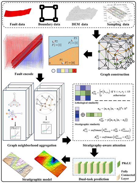
The workflow of the proposed 3D geological modelling method (Geo-SAN), based on a dual-task stratigraphy-aware attention network, is illustrated in Fig. 1. The workflow comprises five key stages, graph construction, graph neighborhood aggregation, stratigraphy-aware attention, lithology classification and implicit interpolation, and 3D geological model reconstruction. The method begins with extracting features from sampled data using the graph neighborhood aggregation and stratigraphy-aware attention mechanisms. Subsequently, a dual-task prediction head is employed to estimate both continuous scalar field values and discrete lithological categories. Finally, the predicted result is integrated to construct a coherent 3D geological model.

Figure 1 Workflow of Geo-SAN.

2.1.1 Graph Neighborhood Aggregation

To address the complexity of geological setting and the large volume of geological data inherent in 3D geological modelling, we employ spatial-domain GAT and GraphSAGE to aggregate node features, thereby harnessing the strong nonlinear integration capabilities of GNNs.

Graph Construction

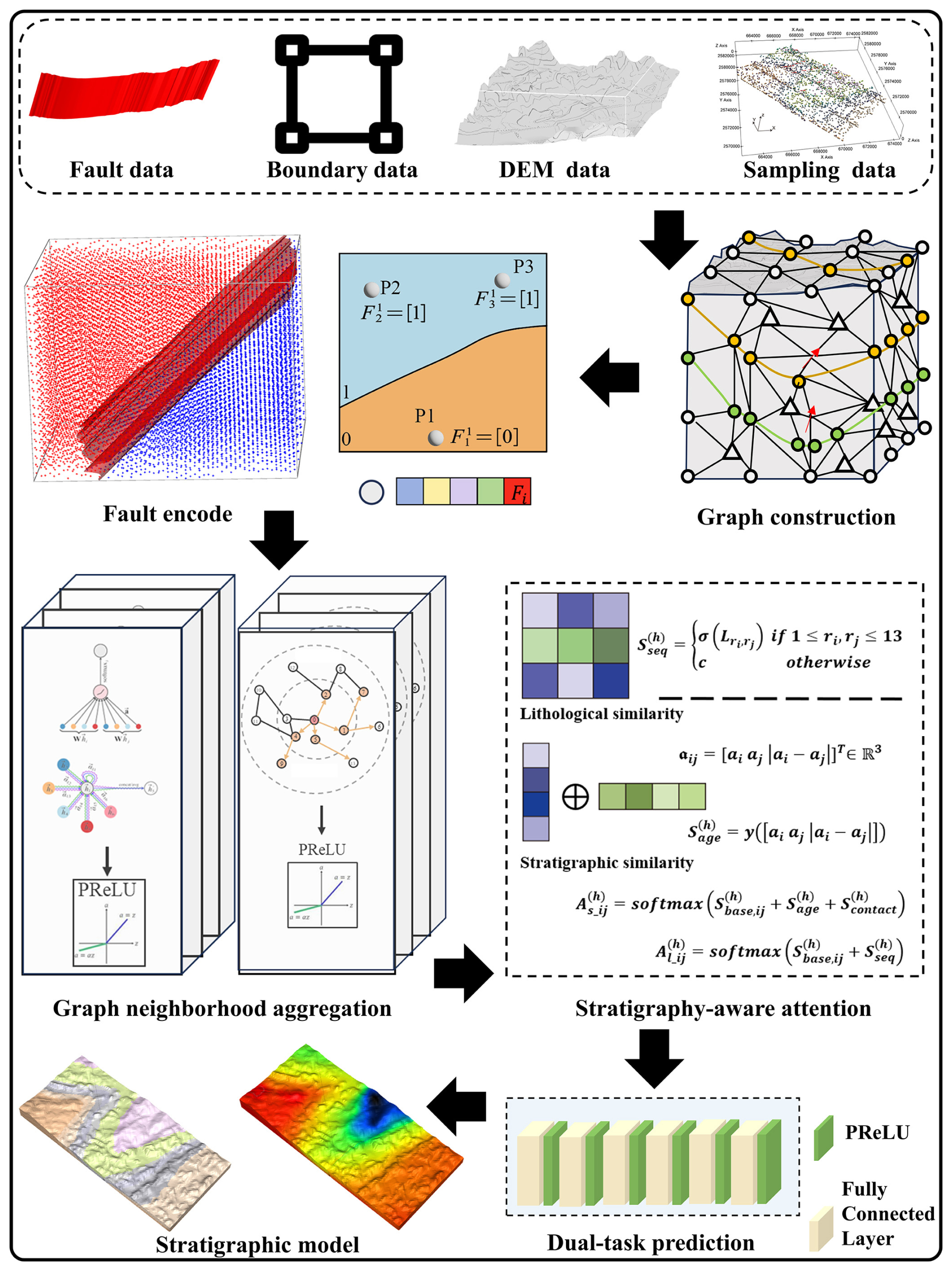
The tetrahedral meshing of the sampled points is performed to create graph structured data. All the sampling points and the other densifying points are both included into the graph data. As shown in Fig. 2, the base and the lateral boundaries are determined by the modeling extent whereas the top boundary is determined by the digital elevation model (DEM). Each sampling point is a vertex of a tetrahedron, and the topological connection of the sampling point is maintained during tetrahedron subdivision. Densifying points are created based on the given modelling resolution; overlapping points are eliminated. The resulting mesh has a multi-resolution structure, with tetrahedra around sampled points having smaller volumes and higher densities. Graph nodes are represented as tetrahedral vertices, and graph edges are represented as tetrahedral edges. Finally, the faults are encoded as a feature of nodes in relation to fault planes, which is combined with other node features as model inputs (Gao and Wellmann, 2025).

Figure 2 Graph construction.

GNN Neighborhood Aggregation

The multi-scale graph neighborhood aggregation mechanism is formulated into the proposed framework. GAT with its learnable attention mechanism gives a specific weight to the neighboring nodes (Veličković et al., 2017), which is especially useful in a geological modeling task where local heterogeneity and sensitivity to the boundaries are considered to be a significant issue. When processing nodes near faults, GAT learns to down-weight connections to neighbors on the opposite side of the fault, effectively preventing spurious propagation of stratigraphic samples across the discontinuity. At stratigraphic boundaries, GAT preferentially attends to aggregate nodes within the same unit, allowing for sharper delineation of geological discontinuities. For node i and its neighbor node j, the attention coefficient α_ij is calculated, which reflects the importance of node j in propagating features to node i, as follows:

$$\begin{array}{}\text{(1)}& {\mathit{\alpha }}_{ij}={\displaystyle \frac{\exp \left(\text{LeakyReLU}\right({\mathit{a}}^T[\mathbf{W}{\mathit{h}}_{\mathit{i}}\Vert \mathbf{W}{\mathit{h}}_{\mathit{j}}]\left)\right)}{{\sum }_{k\in \mathcal{N}\left(i\right)}\exp \left(\text{LeakyReLU}\right({\mathit{a}}^T[\mathbf{W}{\mathit{h}}_{\mathit{i}}\Vert \mathbf{W}{\mathit{h}}_{\mathit{k}}]\left)\right)}}\end{array}$$

where a is the learned attention parameter vector, ‖ represents the concatenation of feature vectors, W is the weight matrix, and h_i and h_j are the feature representations of nodes i and j, respectively.

GraphSAGE statistically incorporates neighboring node features into the central node through a mechanism primarily designed to capture regional geological characteristics and spatial continuity patterns (Hamilton et al., 2017). For scalar value prediction tasks, this approach demonstrates robust capability in capturing spatial gradient patterns, given that scalar properties within a continuous domain generally exhibit gradational transitions rather than abrupt discontinuities. In lithology classification tasks, GraphSAGE exploits the geological principle that spatially proximate nodes tend to share similar features, thereby incorporating the lithological distribution within the statistical neighborhood to inform classification decisions at each target node. GraphSAGE aggregates the features of neighboring nodes layer by layer through a multi-layer neural network, with the embedding update formula for each layer's nodes, as follows:

$$\begin{array}{}\text{(2)}& \begin{array}{rl}& {\mathit{h}}_v^k=\mathit{\sigma }({\mathbf{W}}^k\cdot {\text{AGGREGATE}}_k(\mathit{\{}{\mathit{h}}_{\mathrm{1}}^{k-\mathrm{1}},\forall u\in \mathit{N}(\mathit{v}\left)\mathit{\right\}})\oplus {\mathit{h}}_v^{k-\mathrm{1}})\\ & (k=\mathrm{1},\mathrm{\dots },K)\end{array}\end{array}$$

where ${\mathit{h}}_v^k$ is the embedding vector of node v at the k layer, N(v) is the neighborhood of node v, and AGGREGATE_k is the aggregation function of the k layer. Common choices for aggregation functions include pooling aggregation and long short-term memory (LSTM) aggregation. Given the similarity of geological features within the same region in geological modeling, the average pooling aggregation function is used in this study to embed the features. W^k represents the learnable weight matrix, and ⊕ denotes the vector concatenation operation.

2.1.2 Stratigraphy-Aware Attention Network

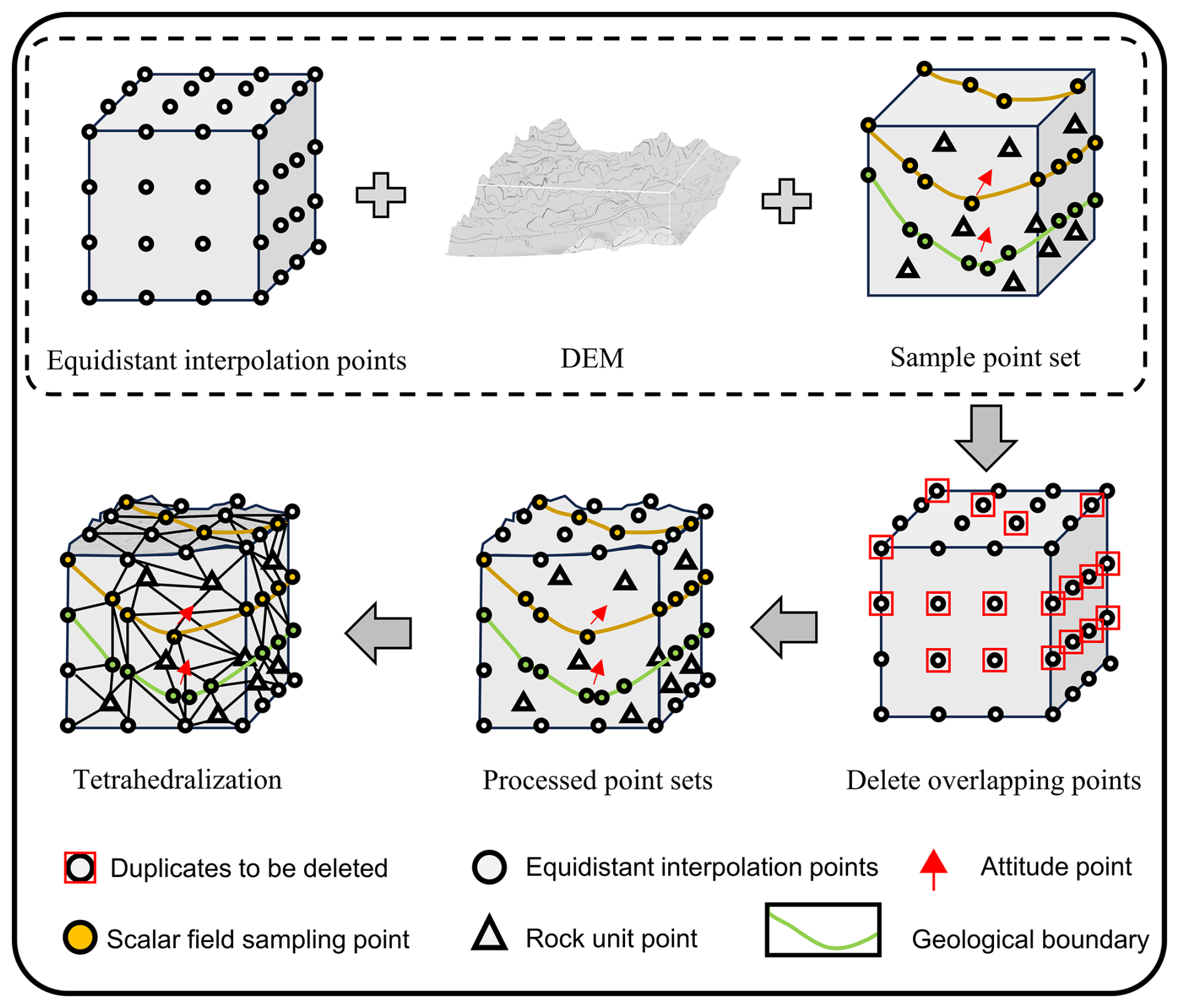
Geological data are distinguished by a high degree of spatial heterogeneity, thereby similar characteristics in different geological environments may have entirely distinct meanings. Such domain-specific subtleties are not reflected in conventional attention mechanisms, which only compute weights using feature similarity. To address this weakness, we present a stratigraphy-aware attention (SAN) process that involves the prior constraints of stratigraphic sequences. Through the incorporation of lithological similarity and stratigraphic sequence, the mechanism gains a meaningful combination of stratigraphy knowledge for the proposed framework (Fig. 3).

Figure 3 Stratigraphy-aware attention network.

First, the SAN receives the following inputs: features aggregated from the graph neighborhood, query vectors Q derived from graph nodes, observation point features K from the graph, and feature V used for aggregation. The input features undergo an initial linear transformation that projects them into the attention space. Secondly, the projected features are partitioned into H attention heads, each processing $d_k=d/\mathit{H}$ dimensional features. For nodes i and j, the base score of the h head is:

$$\begin{array}{}\text{(3)}& S_{\text{base},ij}^{\left(h\right)}={\displaystyle \frac{\mathrm{1}}{\sqrt{d_k}}}{\sum }_{l=\mathrm{1}}^{d_k}{\mathit{Q}}_{i,h,l}\cdot {\mathit{K}}_{j,h,l}\end{array}$$

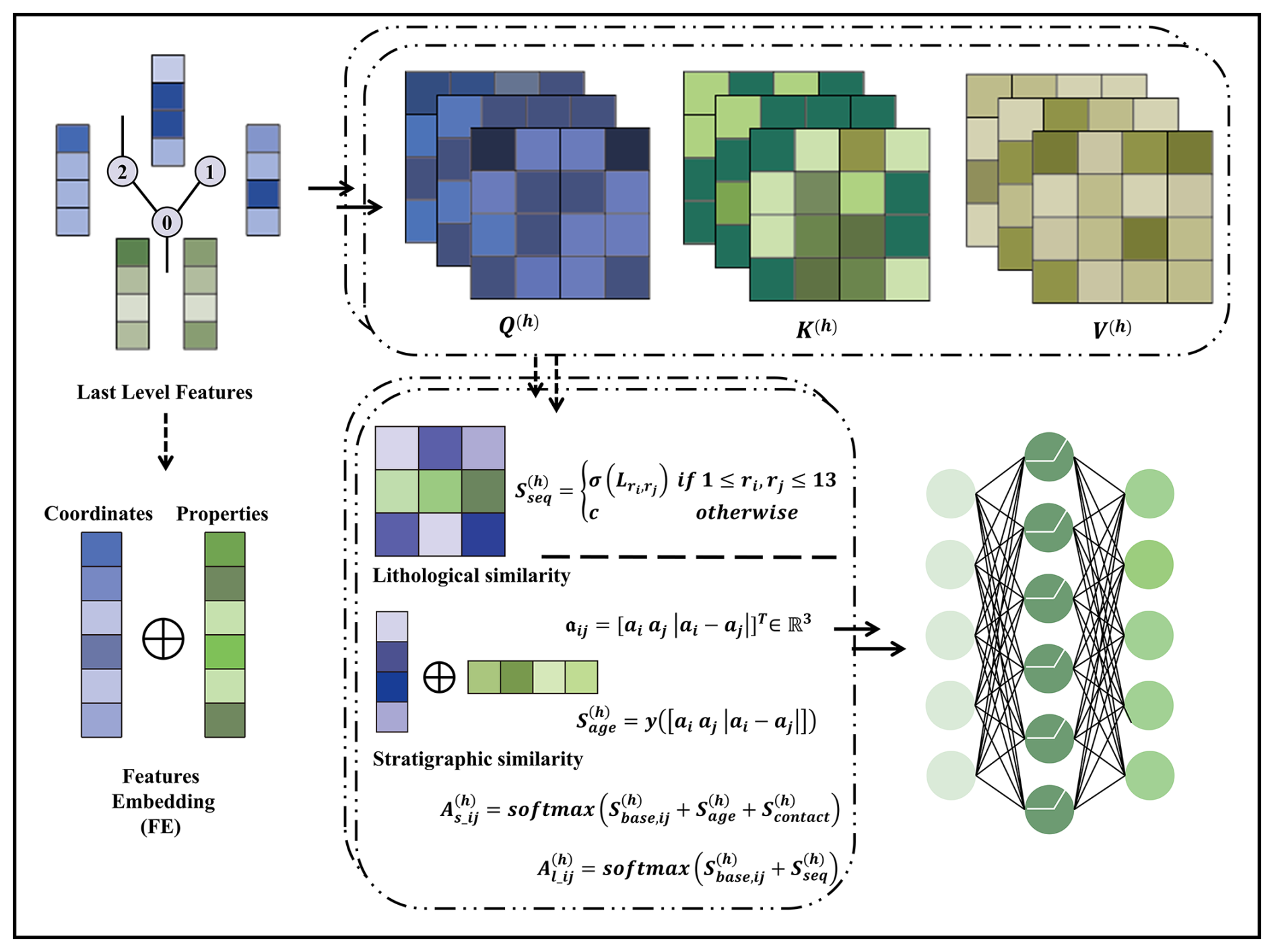
We first define the mapping function from lithology to geological age as a_i=Age(rⁱ), as shown in Fig. 4. For node (i,j), the output $S_{\text{age}}^{\left(h\right)}$ denotes the value for stratigraphic age similarity between node (i,j) at the h head, as follows:

$$\begin{array}{}\text{(4)}& S_{\text{age}}^{\left(h\right)}(i,j)=y\left(\right[a_i{a}_j|a_i-a_j|\left]\right)\end{array}$$

where y(⋅) is the age mapping function.

Figure 4 Stratigraphic similarity.

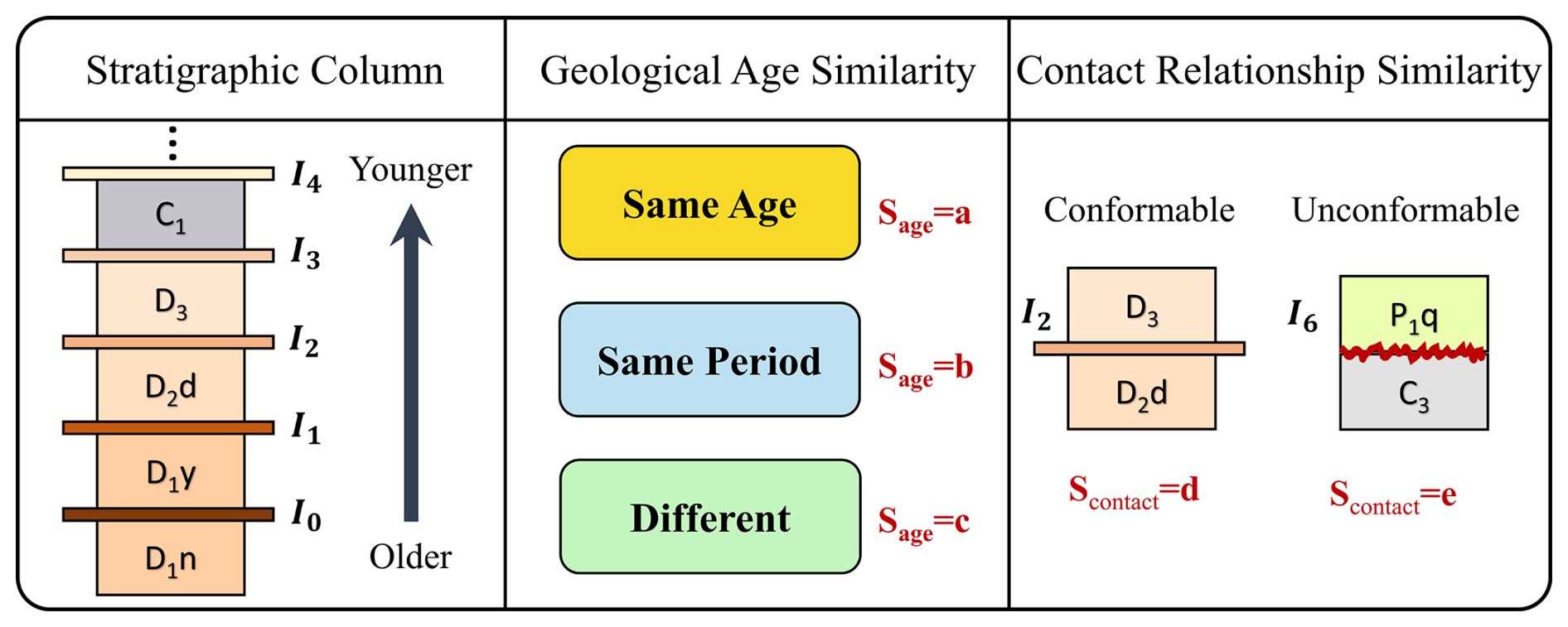
Then, we define a learnable lithological similarity matrix $\mathit{L}\in {\mathbb{R}}^{K\times K}$, where K is the number of lithological categories. Adjacent strata show stronger lithological similarity, with stratigraphic quantitative difference correlating inversely to lithological resemblance. For nodes i and j, lithological similarity S_seq is:

$$\begin{array}{}\text{(5)}& {\displaystyle }{S}_{\text{seq}}^{\left(h\right)}(i,j)=\left\{\begin{array}{ll}\mathit{\sigma }\left(L_{r_i,r_j}\right)& \text{if }\mathrm{1}\le r_i,r_j\le K\\ c& \text{otherwise}\end{array}\right.\end{array}$$

where $\mathit{\sigma }\left(x\right)=\exp (-d(i,j)/\mathit{\tau })$, and $d(i,j)=|i-j|$ denotes that the quantitative difference between the ordinal numbers of two lithological categories within the stratigraphic sequence, and τ is a stratigraphic decay length governing how rapidly lithological affinity is lost with increasing stratigraphic separation. Setting τ=3 assigns adjacent units a similarity of $e^{-\mathrm{1}/\mathrm{3}}\approx \mathrm{0.72}$ and units three steps apart $e^{-\mathrm{1}}\approx \mathrm{0.37}$, which is consistent with the initialized similarity structure recovered in Fig. 5.

Figure 5 Lithological similarity matrix.

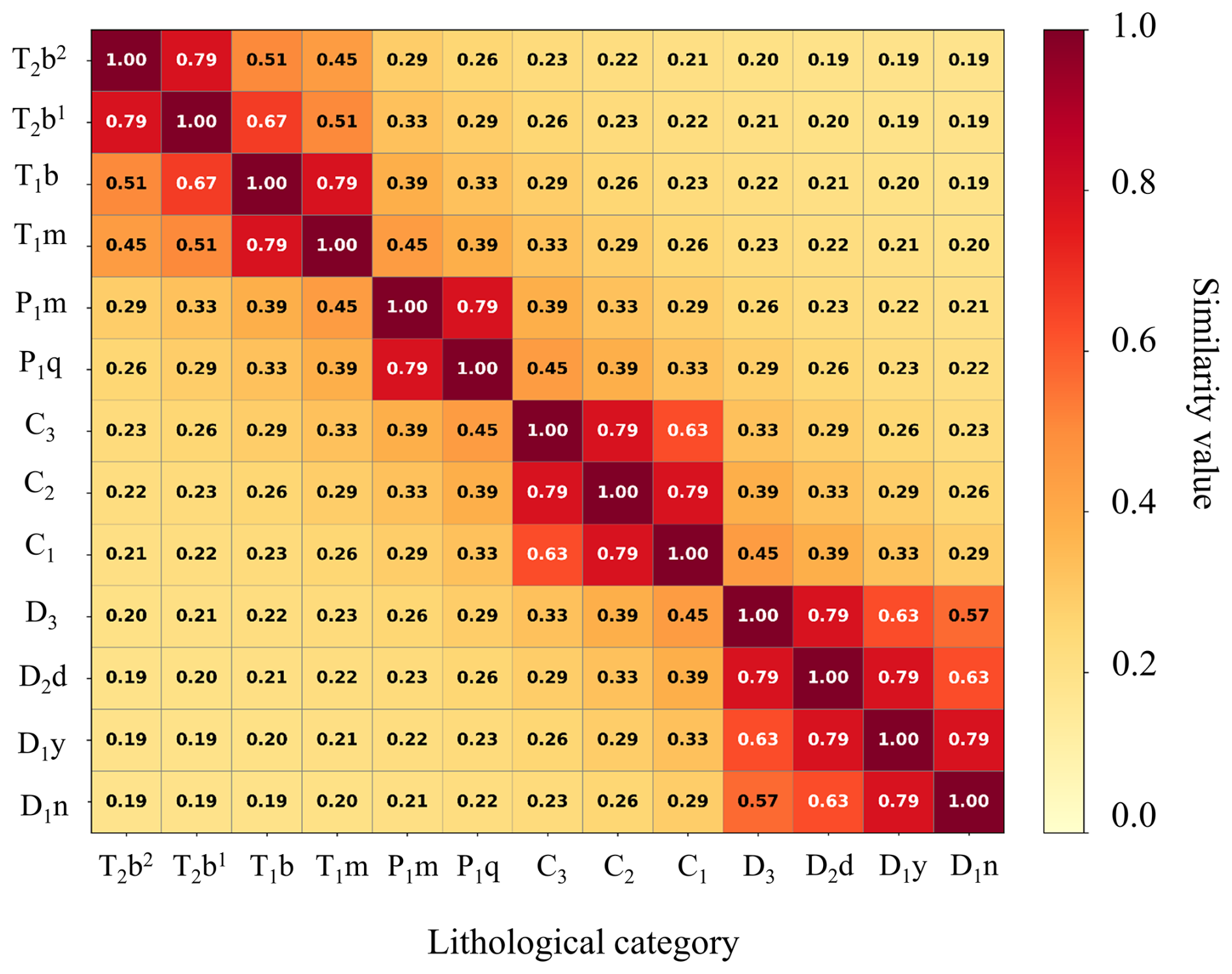
When predicting scalar values, for the h attention head, the enhancing attention for node pair (i,j) is as follows:

$$\begin{array}{}\text{(6)}& A_{s\mathit{\_}ij}^{\left(h\right)}=\text{softmax}\left(S_{\text{base},ij}^{\left(h\right)}+S_{\text{age}}^{\left(h\right)}+S_{\text{contact}}^{\left(h\right)}\right)\end{array}$$

where $S_{\text{contact}}^{\left(h\right)}$ is the similarity of adjustable contact relationship.

When lithology classification, for the h attention head, the enhancing attention for node pair (i,j) is as follows:

$$\begin{array}{}\text{(7)}& A_{l\mathit{\_}ij}^{\left(h\right)}=\text{softmax}\left(S_{\text{base},ij}^{\left(h\right)}+S_{\text{seq}}^{\left(h\right)}\right)\end{array}$$

The SAN mechanism begins by computing standard base attention scores through linear projection of node features and their division into multiple attention heads. Its key innovation is the concurrent incorporation of stratigraphic sequence domain knowledge as prior constraints. For any node pair (i,j), where S_base is the standard query key feature similarity used by conventional attention, S_age is an explicit function of the geological ages of the two nodes' lithologies, S_seq is the learnable lithological similarity that decays with ordinal stratigraphic distance, and S_contact encodes the conformable or unconformable contact relationship. Because these terms are added before the softmax, each attention weight admits an exact additive attribution into a learned feature similarity component and named stratigraphic prior components; the contribution of every prior to any aggregation is therefore transparent and auditable. The two prior terms are monotone in geological proximity. S_age and S_seq raise the weight for node pairs that are close in the stratigraphic sequence and lower it for distant pairs. After the softmax, aggregation is thus biased toward stratigraphically coherent neighbours irrespective of incidental feature resemblance. When S_base is ambiguous (two candidate neighbours with similar features but on opposite sides of a fault or across an unconformity), the prior terms dominate the sum and steer attention to the geologically correct neighbour, which is the mechanism by which cross fault propagation is suppressed and within unit aggregation is sharpened.

2.1.3 Dual-Task Prediction Module

Following the extraction of spatial perceptual features by the SAN, a dual-task learning head is employed to simultaneously perform lithology classification and scalar field prediction, as illustrated in Fig. 6.

Figure 6 Dual-task of lithology classification and scalar field prediction.

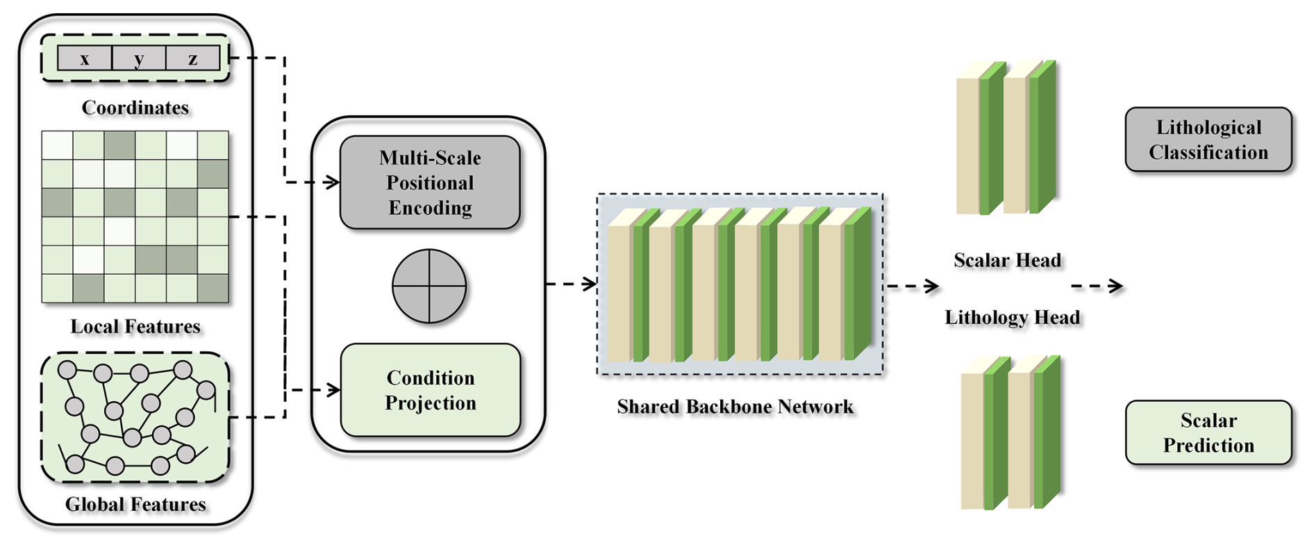
The two branches are coupled at three levels rather than merely sharing a backbone. (1) Reading the same SAN-refined node embedding, so gradients from the two tasks jointly shape the shared representation, forcing features to be simultaneously predictive of the scalar value and of the lithology. (2) The stratigraphy-aware attention injects lithological similarity, geological-age and contact similarity, so the aggregation is tied to stratigraphic structure for both tasks. (3) The cross-task loss explicitly links the two predictions, the KL term (soft) aligns the classifier distribution with the distribution implied by the predicted scalar field, and the compatibility term (hard) penalises scalar predictions that fall outside the admissible interval of the predicted lithology.

2.2 Loss Functions

Three-dimensional geological modeling is a quintessential multi-constrained optimization issue. This study developed the scalar field loss function (ℒ_scalar), attitude loss function (ℒ_orientation), lithology category loss function (ℒ_litho) and scross-task loss function (ℒ_cross). Figure 7 demonstrates ℒ_scalar measures the discrepancy between the observed scalar value S_v at a sampling point and the predicted scalar value $S_v^{\text{scalar}}$ produced by Geo-SAN. The lithological loss ℒ_litho quantifies the disparities between the actual lithological labels and the predicted categories of the model. ℒ_orientation evaluates the discrepancy between the measured direction at orientation sampling points and the direction derived obtained from the predicted scalar field at the corresponding nodes. ℒ_cross converts lithological similarity metrics of stratigraphic sequence into differentiable restrictions, directing neural networks to acquire predictions aligned with stratigraphy principles. The a priori probability distribution of each lithological categories can be computed and determined according to predicted scalar values. Lithological predictions of the model are then regularized to the prior model with the help of the Kullback-Leibler (KL) divergence penalty, which serves as a soft probabilistic constraint. Meanwhile, a compatibility loss term imposes strict penalties on scalar field predictions falling outside the stratigraphically admissible intervals for corresponding lithological categories. Thus, the cross-task constraint may enforce consistency with stratigraphic sequences to yield geologically meaningful predictions.

Figure 7 Loss functions.

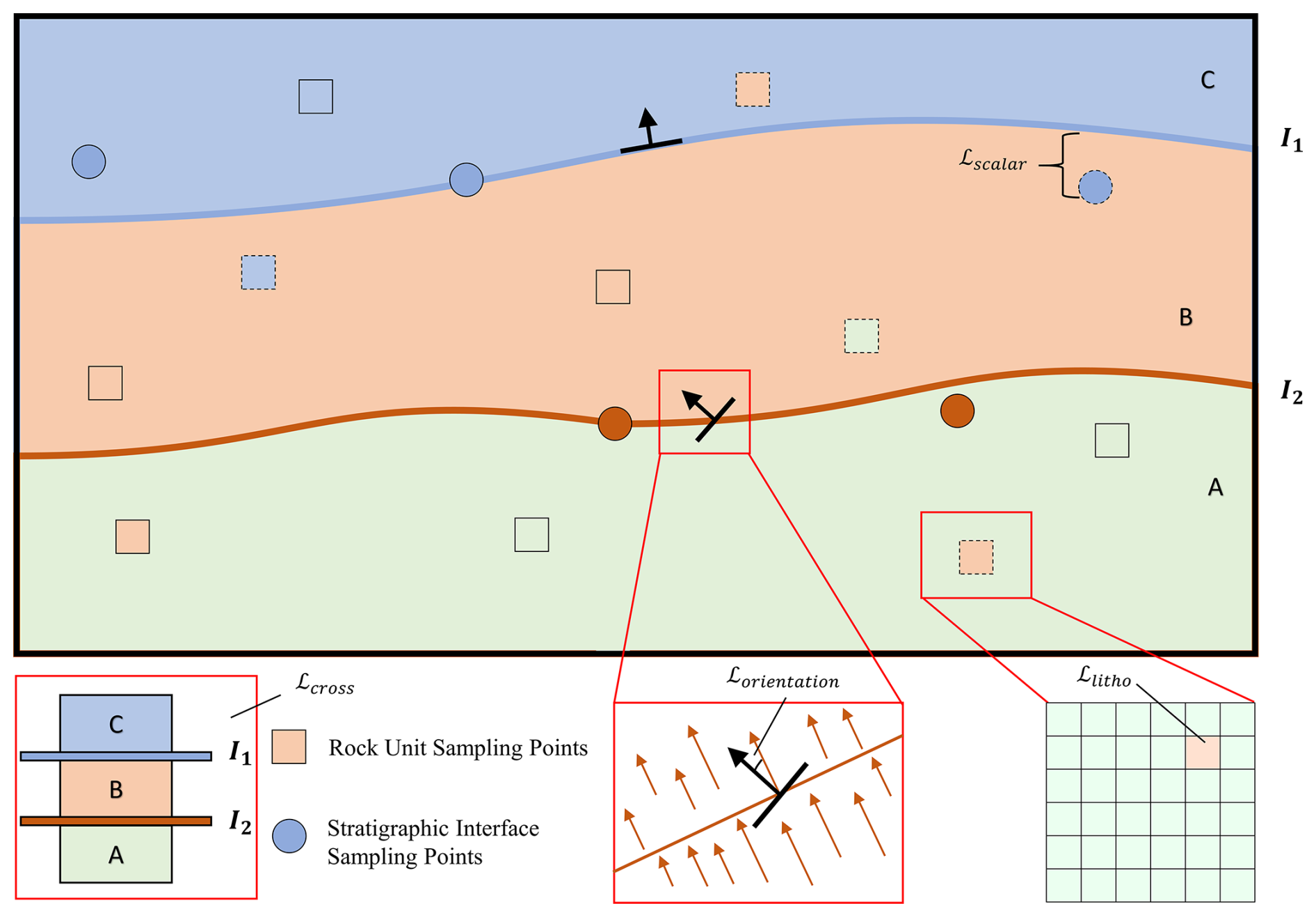
2.2.1 Scalar Field Loss Function

Geo-SAN predicts the scalar field f_v, which is constrained by stratigraphic interfaces and orientation points like dip angle and strike. We can define 3D space as a scalar function f(v), where represents the scalar field values at each point v in 3D space. A series of H stratigraphic interfaces can be articulated as:

$$\begin{array}{}\text{(8)}& f_{\mathrm{1}}>\mathrm{\cdots }>f_H\end{array}$$

where f₁ to f_H represent the scalar values of the oldest to newest stratigraphic interfaces, respectively.

For a certain stratigraphic interface I with a scalar field value f_I, the subset of graph nodes sampled from it can be denoted as:

$$\begin{array}{}\text{(9)}& I=\mathit{\{}v\in \mathit{V}|f_v=f_I\mathit{\}}\end{array}$$

The loss functions ℒ_scalar can be used to find the difference between the scalar field at the stratigraphic interface sampling point and the predicted scalar field by Geo-SAN, as follows:

$$\begin{array}{}\text{(10)}& {\mathcal{L}}_{\text{scalar}}={\displaystyle \frac{\mathrm{1}}{N}}{\sum }_{i=\mathrm{1}}^N({\widehat{f}}_i-f_i{)}^{\mathrm{2}}\end{array}$$

2.2.2 Attitude Loss Function

Nodes with attitudes can be extracted from geological maps, which represent the local morphology of the strata at these nodes. A unit vector n in the normal direction of the stratigraphic interfaces can be transformed from the attitudes:

$$\begin{array}{}\text{(11)}& \mathit{n}=\left[\begin{array}{c}\sin \mathit{\theta }\cdot \sin \mathit{\delta }\\ \cos \mathit{\theta }\cdot \sin \mathit{\delta }\\ \cos \mathit{\delta }\end{array}\right]\end{array}$$

where θ and δ are the strike and dip angles of the stratum, respectively.

To measure predicted gradient and the actual direction of angular error, the gradient of the predicted scalar field is gained at these graph nodes. This study employs the first-order Taylor series approximation of the scalar field in the node's first-order neighborhood to estimate the scalar field gradient, as follows:

$$\begin{array}{}\text{(12)}& {\mathit{P}}_v^T{\mathit{P}}_v\mathbf{\nabla }{f}_v={\mathit{P}}_v^T\left[\begin{array}{c}{f}_u-f_v\\ \mathrm{⋮}\end{array}\right]\end{array}$$

where the angle between the gradient at node v and the known vector $\mathbf{\nabla }{f}_v=(\partial f_v/\partial x,\partial f_v/\partial y,\partial f_v/\partial z)$ can be used to measure the angular error, and u is the neighbor of node v.

$$\begin{array}{}\text{(13)}& {\mathit{P}}_v=\left[\begin{array}{ccc}{x}_u^{\ast }-x_v^{\ast }& y_u^{\ast }-y_v^{\ast }& z_u^{\ast }-z_v^{\ast }\\ \mathrm{⋮}& \mathrm{⋮}& \mathrm{⋮}\end{array}\right],\forall u\in {\mathit{N}}_v\end{array}$$

where x^∗, y^∗, and z^∗ are the normalized spatial coordinates of the given node.

The estimated angle between the gradient ∇f_v at node v and the known vector α_v in the observed attitude node-set o is utilized to formulate the loss function, as follows:

$$\begin{array}{}\text{(14)}& \begin{array}{rl}{\mathcal{L}}_{\text{orientation}}& ={\sum }_{v\in o}\cos \left(\mathbf{\nabla }{f}_v,{\mathit{\alpha }}_v\right)\\ & ={\sum }_{v\in o}{\displaystyle \frac{{\mathit{\alpha }}_v\cdot \mathbf{\nabla }{f}_v}{\Vert {\mathit{\alpha }}_v\Vert \Vert \mathbf{\nabla }{f}_v\Vert }}\end{array}\end{array}$$

2.2.3 Lithology Category Loss Function

In the lithology node-set R, comprising N_classes lithology categories, each lithology node is associated with a one-hot encoded vector l_v, denoting its respective lithology category. The loss function employed for lithology nodes is the cross-entropy loss function, as follows:

$$\begin{array}{}\text{(15)}& {\mathcal{L}}_{\text{litho}}=-{\sum }_{v\in R}({\mathit{l}}_v\cdot \log ({\widehat{\mathit{l}}}_v\left)\right)\end{array}$$

where ${\widehat{\mathit{l}}}_v$ is the predicted probability distribution for node v, and the predicted lithology category is determined based on the highest probability from the softmax distribution of ${\widehat{\mathit{l}}}_v$.

2.2.4 Cross-Task Loss Function

The KL divergence loss function (soft constraint) is utilized to measure the discrepancy between lithology classification and scalar field prediction, thus encouraging models to adhere to stratigraphic sequence patterns, as follows:

$$\begin{array}{}\text{(16)}& {\mathcal{L}}_{\text{KL}}=\text{KL}(\widehat{\mathit{l}}\Vert \widehat{\mathit{l}\mathit{f}})={\sum }_{i=\mathrm{1}}^N{\sum }_{j=\mathrm{1}}^K{\widehat{\mathit{l}}}_i^j\log {\displaystyle \frac{{\widehat{\mathit{l}}}_i^j}{{\widehat{\mathit{l}\mathit{f}}}_i^j}}\end{array}$$

where ${\widehat{\mathit{l}}}_i^j$ denote that model's predicted probability distribution over jth lithological category at ith node, and ${\widehat{\mathit{l}\mathit{f}}}_i^j$ denote that the probability distribution derived from stratigraphic scalar field.

The compatibility loss function evaluates whether expected scalar field conform to the acceptable range for lithological category, imposing penalties on forecasts that contravene geological principles, as follows:

$$\begin{array}{}\text{(17)}& {\mathcal{L}}_{\text{compat}}={\displaystyle \frac{\mathrm{1}}{N}}{\sum }_{i=\mathrm{1}}^N\left(\mathrm{1}-\exp \left(-{\displaystyle \frac{\mathrm{\Delta }f\left(i\right)}{F}}\right)\right)\end{array}$$

where F denotes exceeding the upper or lower threshold. The deviation Δf(i) measures how far the predicted scalar value is outside the valid range:

$$\begin{array}{}\text{(18)}& \mathrm{\Delta }f\left(i\right)=max(\mathrm{0},{\widehat{f}}_i-t{l}_i)+max(\mathrm{0},b{l}_i-{\widehat{f}}_i)\end{array}$$

where tl_i and bl_i are the top and bottom interface scalar values according to the observed lithological category at node i. When $b{l}_i\le \widehat{f}\le t{l}_i$, then Δf(i)=0 (perfect compatibility). The cross-task loss function is expressed as:

$$\begin{array}{}\text{(19)}& {\mathcal{L}}_{\text{cross}}={\mathcal{L}}_{\text{KL}}+{\mathcal{L}}_{\text{compat}}\end{array}$$

The overall loss function is as follows:

$$\begin{array}{}\text{(20)}& \mathcal{L}=\mathit{\alpha }{\mathcal{L}}_{\text{scalar}}+\mathit{\beta }{\mathcal{L}}_{\text{orientation}}+\mathit{\gamma }{\mathcal{L}}_{\text{litho}}+\mathit{\delta }{\mathcal{L}}_{\text{cross}}\end{array}$$

In this study, the GradNorm (Gradient Normalization) method is introduced to optimize the training process (Chen et al., 2018). GradNorm adaptively adjusts the weights of each task's loss function to ensure that the gradients of each task have similar magnitudes during training, improving the stability and efficiency of training.

2.3 Experimental Environment

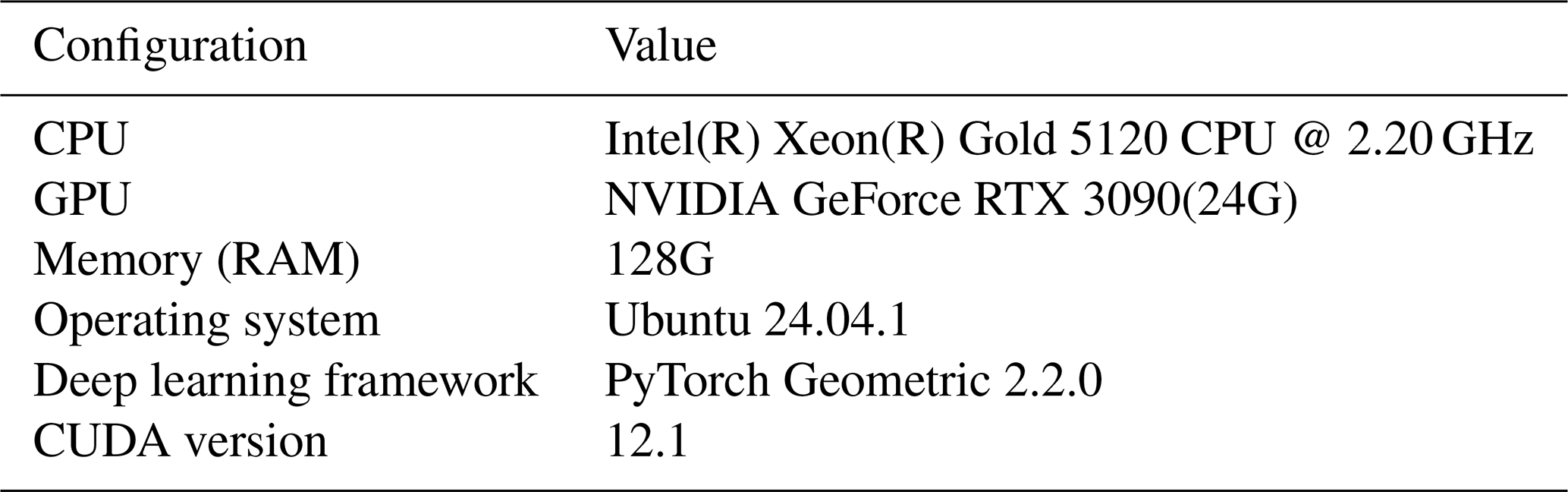
The experiments in this study are based on the PyTorch Geometric graph machine learning library (Fey and Lenssen, 2019), as shown in Table 1.

Table 1 Experimental environmental.

3 Study Area and Dataset

The study area is situated in the Lingnian-Ningping area in Guangxi Zhuang Autonomous Region (GZAR), China (Fig. 8). The area predominantly exhibits strata from the Late Paleozoic onwards, therein, strata from the Late Permian (P₃) and Late Triassic to Pleistocene (T₃–N₂) are absent. The Middle Permian (P₂) and Early Triassic (T₁) strata exhibit parallel unconformity, whereas the Middle Triassic (T₂) and Quaternary (Q) strata display angular unconformity. In the central region of the study area, a left-lateral strike-slip reverse fault, the Nacha Fault, intersects the Maokou Formation and Carboniferous strata, dipping southeast at approximately 70° and extending roughly 12 km outside the study area. Within the area, there exist two synclines (I and III) and one anticline (II). Syncline III, located at the center of the study area, has high symmetry, featuring a northeast-trending axial trace, and is truncated along its southern limb by the Nacha Fault. Anticline II is situated in the northwestern section of the study area, demonstrating a notable symmetry and a northeast-oriented axis. Sampling points for stratigraphic interfaces, lithologies, and attitudes were extracted from a planar and four cross-section geological maps (Fig. 9) to constitute the modeling dataset. There are 1410 stratigraphic interface sampling points, 18 619 lithology sampling points, and 34 attitude points.

Figure 8 Geological map of the study area, modified after Zhang et al. (2023a).

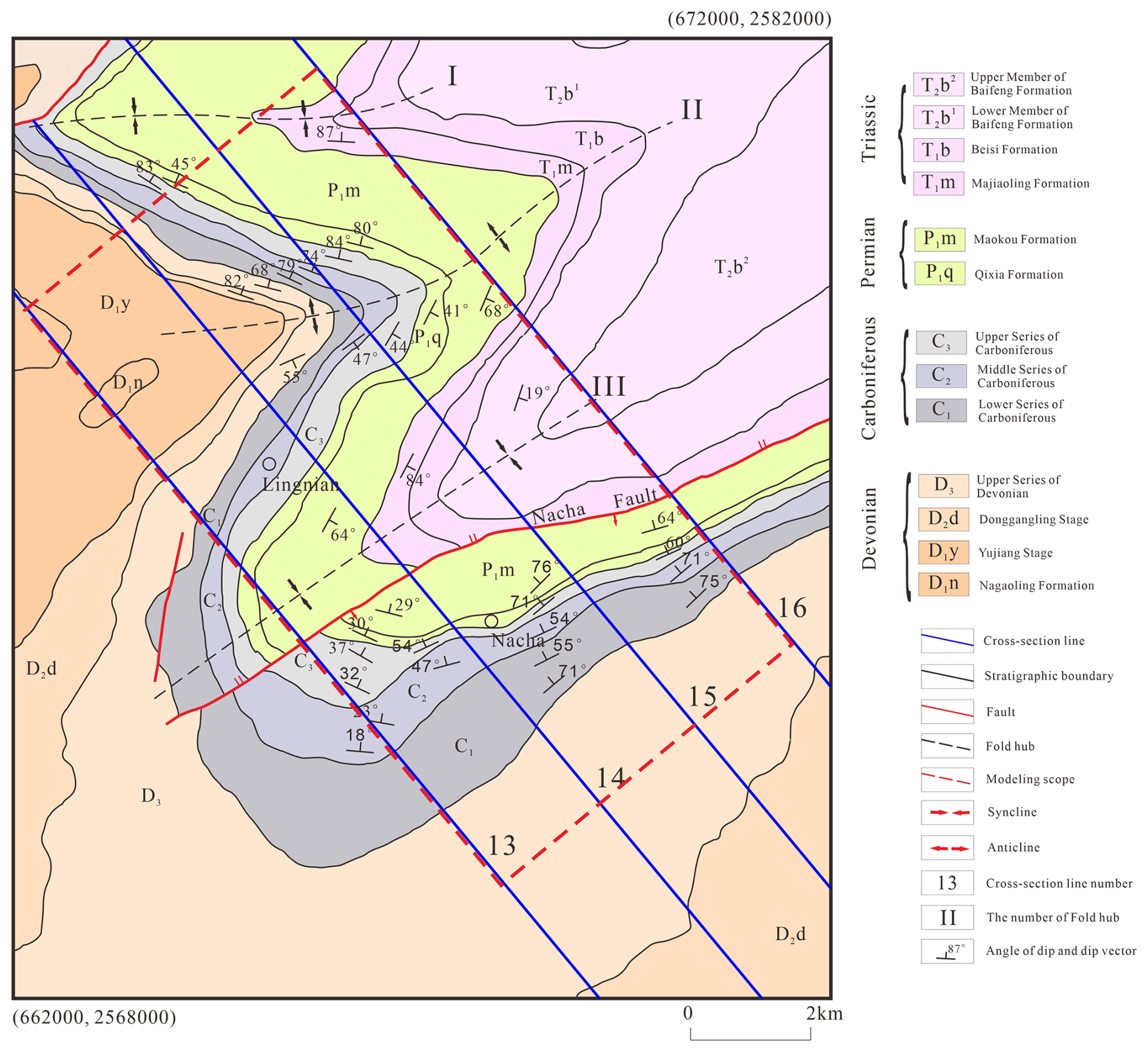
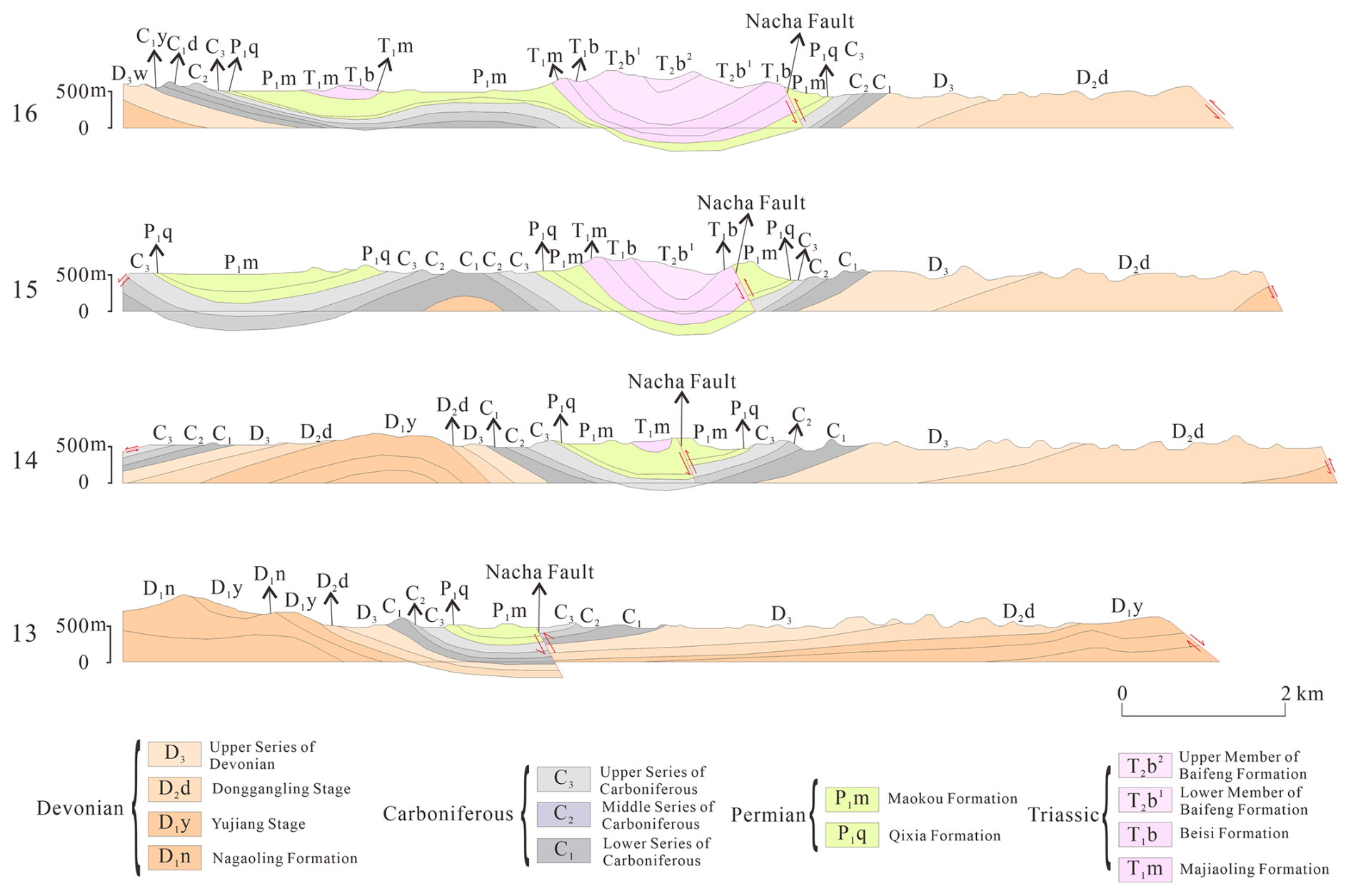
Figure 9 Geological cross-section maps of the study area, modified after Zhang et al. (2023a).

4 Results

4.1 Model Performance

During model training, various configurations significantly affect performance. To isolate the individual contributions of the stratigraphy aware attention (SAN) mechanism and the dual-task learning head, four models were designed on an identical graph neighborhood aggregation backbone that alternately integrates GAT and GraphSAGE, as detailed in Table 2. Model M1 (GAT-GraphSAGE) is the baseline, using only the GAT/GraphSAGE embedding with the two prediction branches trained independently. Model M2 (GAT-GraphSAGE-DT) additionally activates the dual-task cross-task constraint, the KL-divergence and compatibility terms (ℒ_cross) that couple the scalar field and lithology branches, while excluding SAN. Model M3 (GAT-GraphSAGE-SAN) adds the SAN mechanism to the baseline while keeping the two branches decoupled. Model M4 (GAT-GraphSAGE-SAN-DT) incorporates both SAN and the dual-task constraint, constituting the complete Geo-SAN framework. In all configurations both prediction branches are retained, R² and RMSE or accuracy are reported for every model; the Dual-Task toggle controls only whether the cross-task coupling ℒ_cross is applied.

Table 2 Ablation experiments.

The ratio of training dataset to testing dataset is set as 8:2, with all models trained according to hyperparameters specified in Table 3.

Table 3 Model hyperparameters.

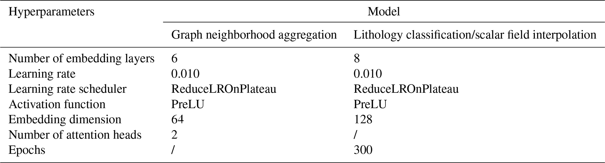
Figure 10 presents scalar field prediction metrics, all four models converge after roughly 300 epochs. Both components improve scalar field interpolation relative to the baseline M1 (R²=0.931, RMSE=0.086): enabling SAN raises R² to 0.961 and lowers RMSE to 0.073 (from M1 to M3), while enabling the dual-task constraint raises R² to 0.955 and lowers RMSE to 0.072 (from M1 to M2). Their effects are complementary, and the full model M4 attains the best result (R²=0.971, RMSE=0.062). The gain from SAN is slightly larger on R², consistent with its explicit injection of stratigraphic age and contact relationship priors, which regularizes the continuous scalar field and yields smoother, more geologically consistent transitions.

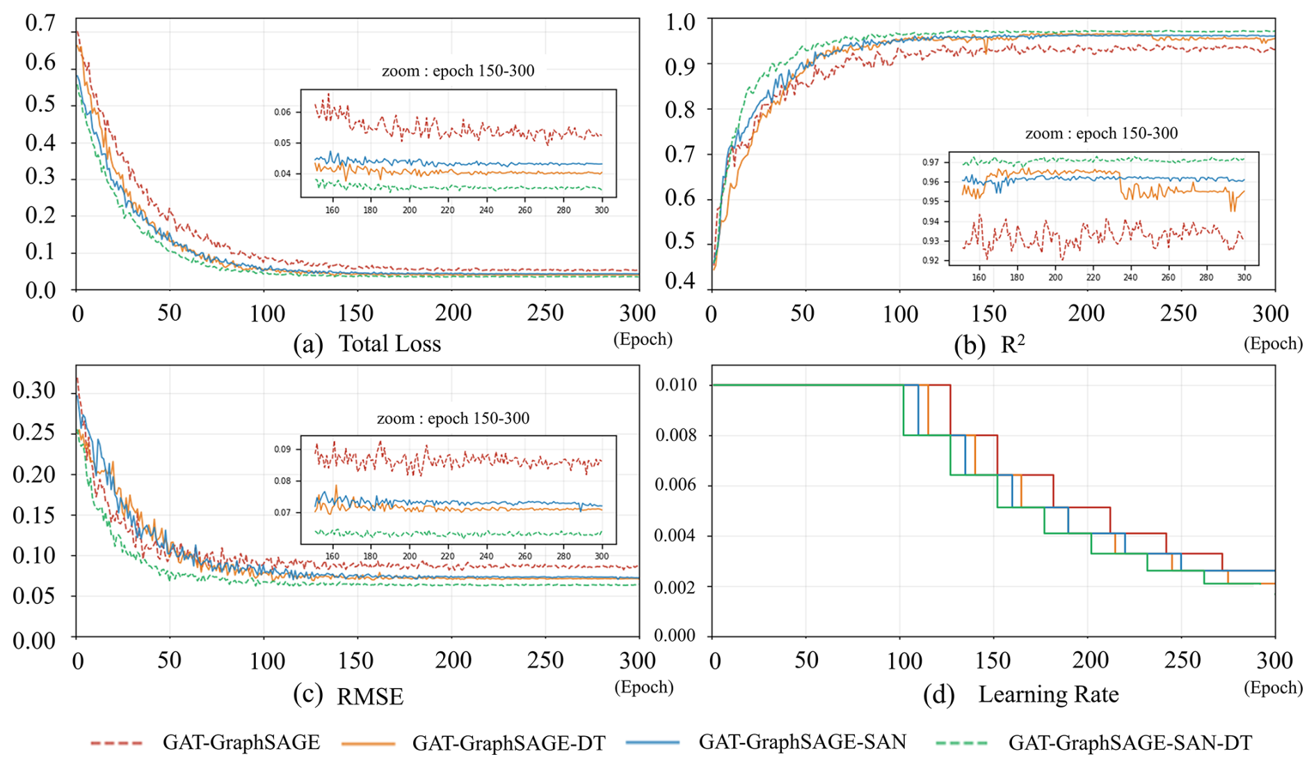
Figure 10 Model evaluation metrics for scalar field interpolation training processes: (a) total loss, (b) R², (c) RMSE, and (d) learning rate.

The lithology classification training curves are shown in Fig. 11. Relative to the baseline M1 (accuracy=0.841), adding the SAN mechanism improves accuracy to 0.879 (from M1 to M3), and with the dual-task constraint, from 0.841 to 0.899 (from M1 to M2), adding the dual-task constraint and SAN mechanism improves accuracy from 0.841 to 0.921 (from M1 to M4). Both factors therefore contribute positively and roughly additively, with the cross-task constraint contributing somewhat more to lithology classification than SAN. The SAN improvement reflects the geological principle that lithologies adjacent in the stratigraphic sequence tend to be similar, explicitly incorporating lithology similarity and stratigraphic sequence constraints. The dual-task improvement reflects the cross-task coupling that regularizes lithological predictions against the stratigraphic scalar field.

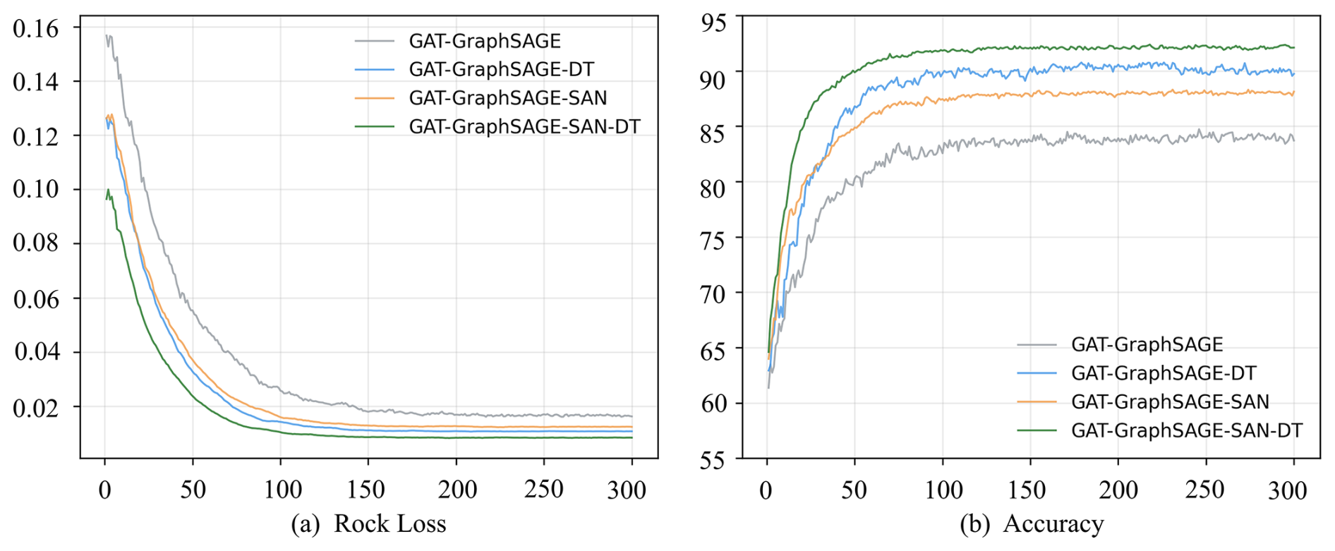
Figure 11 Model evaluation metrics in lithology classification training processes: (a) loss, and (b) accuracy.

To benchmark Geo-SAN against mainstream learning-based interpolators, Table 4 evaluates three standalone GNN backbones, GCN (M5), GAT (M6), and GraphSAGE (M7), each without the SAN prior and without dual-task coupling, on the identical graph, feature set, and sampling split.

Table 4 Comparison experiments.

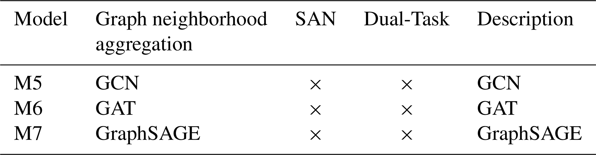
Table 5 summarizes the metrics of the ablation models (M1–M4) and the comparison models (M5–M7). The full model M4 performs best on both tasks (R²=0.971, RMSE=0.062, and accuracy=0.921). Relative to the baseline M1, SAN and the dual-task constraint yield consistent gains but favor different tasks: SAN contributes more to scalar field prediction (M3 vs. M2, R² 0.961 vs. 0.955), whereas the dual-task constraint contributes more to classification (M2 vs. M3, accuracy 0.899 vs. 0.879). The declining cross-task loss shows that the two components reinforce each other, and the 8.0 % accuracy gain of M4 over M1 stems from both jointly rather than from either alone. Under the baseline setting, the single backbone models rank GraphSAGE > GAT > GCN on both tasks (accuracy of 0.828, 0.810, and 0.805; R² of 0.920, 0.904, and 0.879), reflecting the suitability of GraphSAGE's regional aggregation for stratified structures. The alternating GAT+GraphSAGE backbone (M1) surpasses all single backbones (R²=0.931, accuracy=0.841) at comparable cost, confirming that multi-scale aggregation extracts more representative features from sparse and irregular samples.

Table 5 Model performance evaluation metrics (300 epochs).

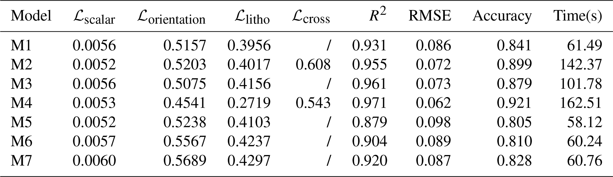
Viewed from the overall architecture, the three modules address complementary bottlenecks: the alternating GAT+GraphSAGE backbone strengthens feature extraction from sparse, irregular samples, the SAN module injects stratigraphic constraints as additive attention terms and thus benefits scalar field interpolation most, while the cross-task loss regularizes the classifier against the predicted scalar field and thus benefits lithology classification most.

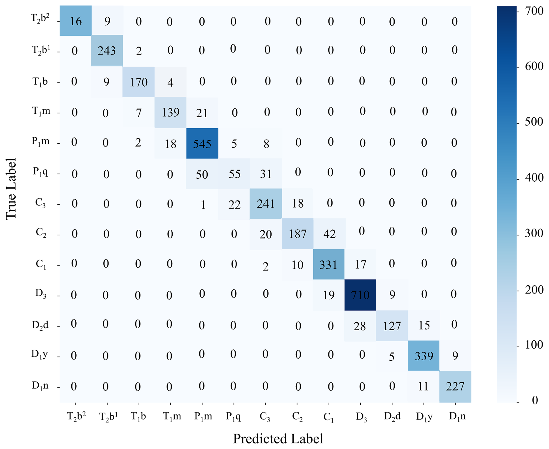
The confusion matrix (Fig. 12) shows that the proposed model performs well in all thirteen lithological categories. The model's highest classification accuracy is for D₃ and P₁m lithologies. T₂b¹, C₃, C₁, D₁y, and D₁n have over 85 % correctly identified samples, demonstrating strong generalization and stable prediction. Although T₁m and P₁m, and D₂d and D₁y are slightly confused, the overall misclassification remains low, learning meaningful feature representations for each lithological category. Results show three major benefits: (1) Thirteen lithological categories are accurately recognized; (2) Most predictions are correctly along the diagonal with few off-diagonal errors; And (3) residual confusion is between lithologies with similar stratigraphic attributes or transitional relationships. The proposed Geo-SAN model performs well in automated lithology classification under complex geological conditions and provides an intelligent foundation for 3D geological modelling.

Figure 12 Geo-SAN lithology classification confusion matrix.

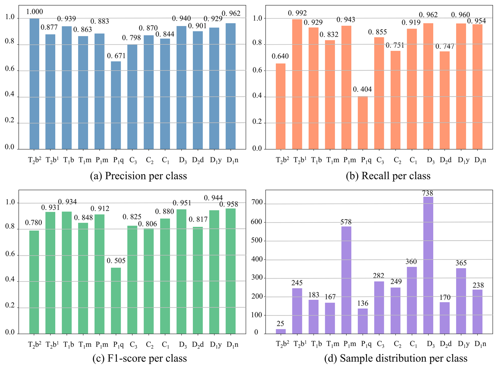
According to category-wise performance metrics (Fig. 13), the model demonstrates well in lithology classification. Most lithological categories have F1-scores above 0.80, with T₂b¹, P₁m, D₃, D₁y, and D₁n having values above 0.90, indicating high classification reliability. Most lithology categories, except P₁q (0.671), have precision between 0.79 and 0.99, indicating good false positive control. Most categories maintain recall values between 0.74 and 0.99, indicating high true positive detection rates. The model's robustness under extreme sample imbalance (25 samples of T₂b² to 738 samples of D₃) is noteworthy. This shows the Geo-SAN architecture's powerful feature-learning capability and the training strategy's efficacy. Although the recall of P₁q is relatively low (0.404), likely due to its feature similarity with adjacent lithologies, the model still achieves F1-scores above 0.82 for most sparse categories, demonstrating strong small-sample generalization. The model exhibits three major strengths: (1) balanced precision and recall, with most lithological categories achieving values above 0.90 for both metrics; (2) high resilience to sampling imbalance, maintaining stable performance even under severely skewed sample distributions; (3) strong lithology classification applicability, with F1-scores ranging from 0.50 to 0.95.

Figure 13 Geo-SAN model lithology classification evaluation metrics.

4.2 Scalar Field

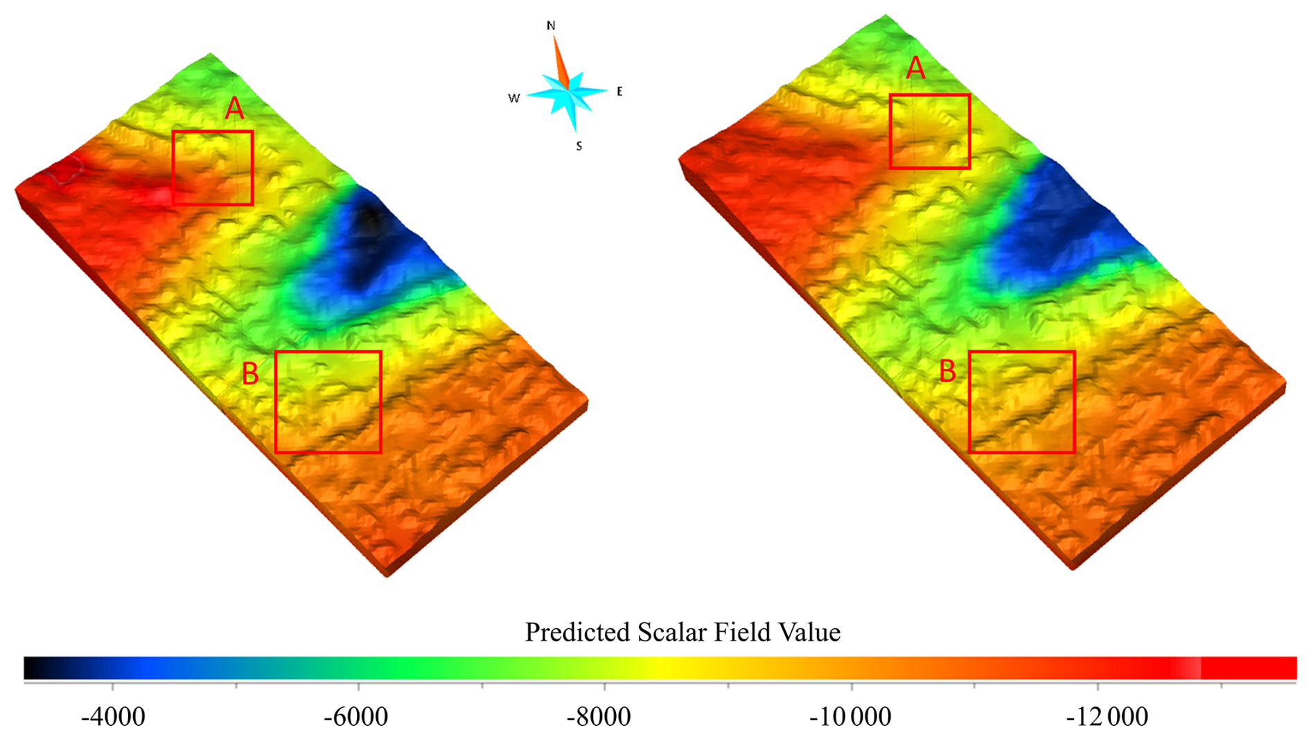
Comparative analysis of scalar fields by Geo-SAN and gradient-adaptive Hermite radial basis function (AdaHRBF) (Zhang et al., 2023a), as shown in Fig. 14, shows that both modeling approaches exhibit a broad consistency of large-scale trends and accurately describes the smooth changes of the scalar fields. The AdaHRBF method creates several inharmonious changes in values of scalar fields in structurally complicated areas that are attributed to uneven distribution of sampling points in the spaces and presence of noise which may lead to instability and local distortion. On the other hand, the scalar field generated by Geo-SAN has more gradual and geological smooth transitions in the same areas. The Geo-SAN method improves robustness and local adaptivity by combining SAN and graph-based neighborhood aggregation, creating more robust scalar field representations in complex geological settings.

Figure 14 Three-dimensional scalar fields modeled by (a) AdaHRBF and (b) Geo-SAN.

4.3 Lithology Classification

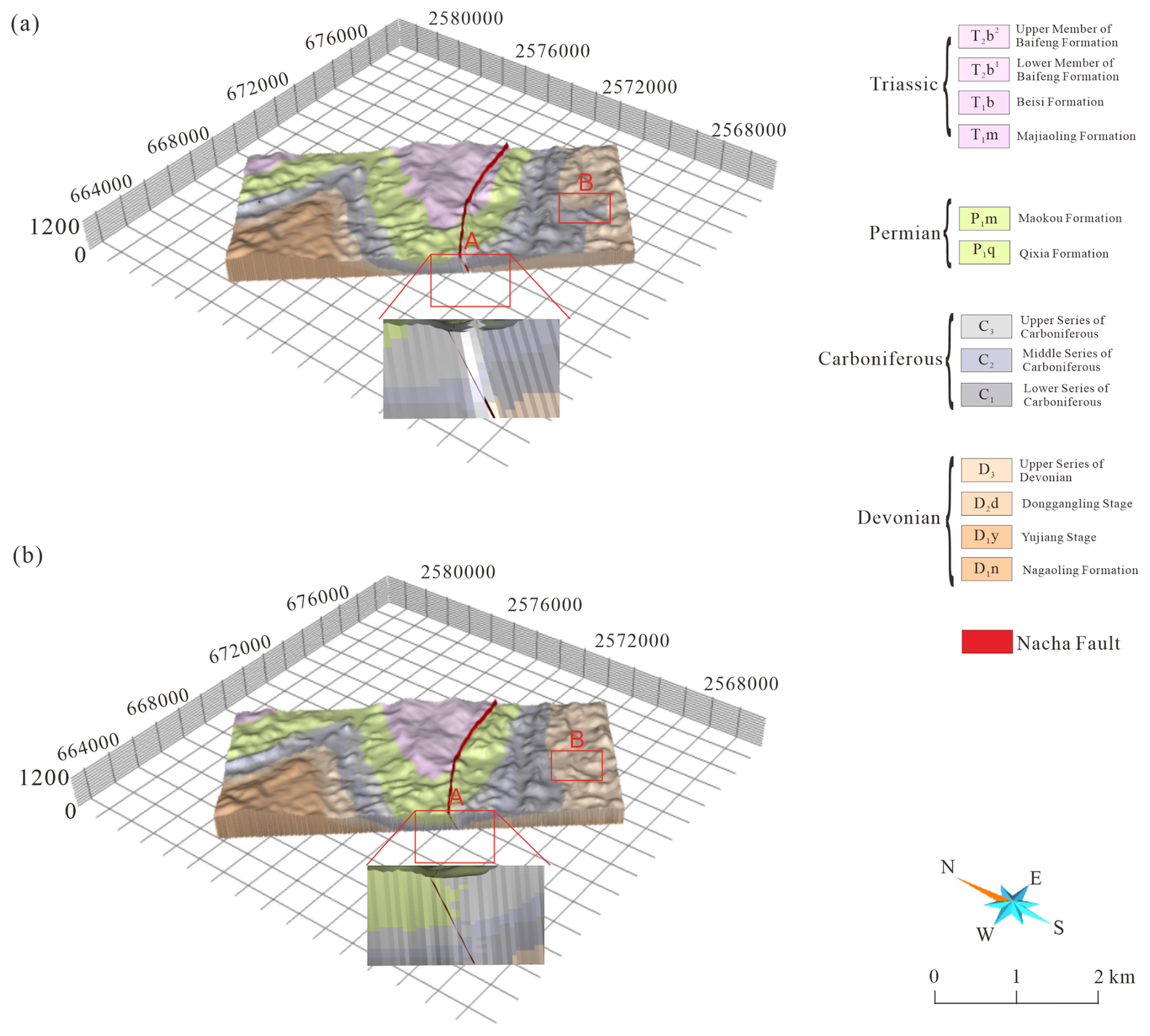
The proposed Geo-SAN method establishes an inherent coupling between scalar field and lithological categories, thereby enabling direct prediction of lithological classes. In contrast, the AdaHRBF method derives lithological categories indirectly through inequalities of scalar field. Constrained by the DEM surface, two stratigraphic models were reconstructed (Fig. 15). Both approaches yield stratigraphic models that reasonably reproduce the major geological structures in the study area, including Synclines I and III and Anticline II. The stratigraphic model generated by the AdaHRBF method, however, has local unnatural stratigraphic forms(marked in red), and high levels of inconsistency in stratigraphic ordering and thickness distribution on both sides of fault-involved areas. In contrast, the Geo-SAN-based model has good stratigraphic continuity within these structurally complex areas and displays no apparent stratigraphic sequence or thickness anomaly.

Figure 15 Three-dimensional stratigraphic models by (a) AdaHRBF and (b) Geo-SAN.

Four geological cross-sections are extracted out of the 3D stratigraphic models by AdaHRBF and Geo-SAN, as shown in Fig. 16. Cross-sections gained in the AdaHRBF model indicate unnatural stratigraphic forms that show pronounced inequalities in stratigraphic sequence and changes in thickness on both sides of fault-involved areas. Conversely, the Geo-SAN approach exhibits remarkable stratigraphic consistency in these regions, with no discernible sequence flaws.

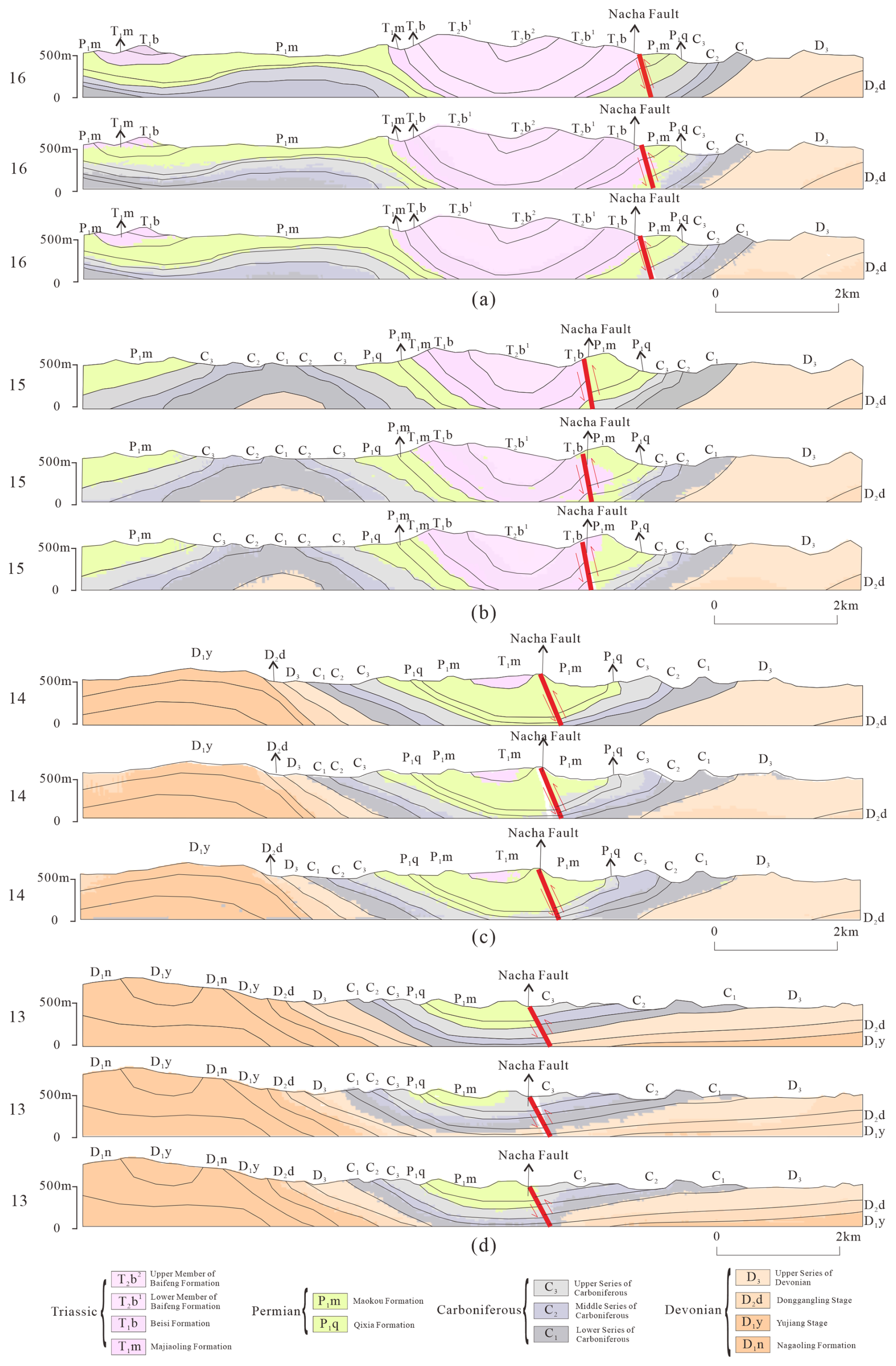
Figure 16 Compare the cross-section nos. of (a) 16, (b) 15, (c) 14, and (d) 13 generated by actual, AdaHRBF and Geo-SAN models.

5 Discussions

This study presents a 3D geological modelling framework, Geo-SAN, which is founded upon a dual-task stratigraphy-aware attention network. Unlike conventional implicit modelling methods, which rely on interpolation algorithms and the solution of large-scale linear equations, the suggested method utilizes the message-passing capabilities of GNNs to obtain the multi-scale aggregation of geological data, which is highly effective in overcoming the spatial modelling issues of sparse and irregular sampling points. The scheme is capable of dynamically modifying its feature aggregation strategy based on the lithological similarity and stratigraphic relationship so that a smooth incorporation of data-driven learning and knowledge-driven stratigraphic sequence constraints can be incorporated.

Among NNG approaches, CNNs require resampling onto regular grids (Bi et al., 2022; Zhang et al., 2024), and MLPs discard explicit topology (Chu et al., 2024; Hillier et al., 2023), whereas GNNs retain irregular sampling topology (Hillier et al., 2021; Gao and Wellmann, 2025; Liao et al., 2026); in all of these, however, aggregation weights derive from feature similarity alone and the prediction branches are not explicitly coupled. Under an identical graph, feature set, and sampling split, Geo-SAN improves R² from 0.920 to 0.971 and accuracy from 0.828 to 0.921 relative to the strongest single backbone (GraphSAGE, M7), indicating that the gain originates from the stratigraphic priors and the cross-task coupling rather than from the backbone itself.

Ablation experiments further disentangle the two proposed components: the SAN mechanism contributes 2.2 %–3.8 % and the dual-task constraint 4.2 %–5.8 % to lithology classification accuracy, together accounting for the 8.0 % improvement of the full model over the baseline. This underscores the complementary roles of stratigraphic sequence prior knowledge and cross-task coupling in constraining feature aggregation and improving model robustness.

Despite these advances, there are still several limitations. First, the cross-task constraint narrows but does not eliminate this overlap where some ambiguity is irreducible where lithologies are genuinely similar and contacts are gradational. This is consistent with geological reality and delimits the scope of the coupling. Second, a closed set supervised classifier can only predict lithologies present in the training set. For a stratigraphic unit absent from the training data, the current model would then assign it to the nearest known class. Third, the existing framework is highly developed to stratified geological bodies and its applicability to more complex geological structures, including igneous intrusions, salt domes, and heterogeneous mixed rocks, has not been confirmed. Fourth, faults are encoded as a one-hot node feature, which marks the presence of a discontinuity but does not represent fault displacement, fault type (normal, reverse, or strike-slip), or the detailed offset across the fault. Therefore, future improvements are suggested on: (1) active learning to optimize sampling strategy and minimize reliance on the spatial distribution of dataset, (2) handling this “untrained-unit” case requires open-set recognition (flagging out-of-distribution nodes as “unknown”), semi-supervised or self-training strategies, or continual/transfer learning, (3) adding structural constraint pattern or modeling strategies that use topological relationships to better express irregular boundaries, complicated contact relationships, and spatial topology, and (4) for oblique-slip structures such as the Nacha Fault, encoding the slip vector and displacement magnitude, thereby further improving the prediction of near fault stratigraphic thickness.

6 Conclusions

This study addresses the computational inefficiency, limited capacity for constraint integration, and inadequate treatment of spatial discontinuities commonly encountered by traditional geological implicit modelling methods when dealing with complex geological structures. We introduce a 3D geological modelling framework, Geo-SAN, which consists of a dual-task stratigraphy-aware attention network, and allows the joint optimization of lithology classification and scalar field interpolation. The proposed method obtains a lithology classification accuracy of 92.1 % and an R² of 0.971 to predict scalar field.

The principal contributions of the study include the following: (1) A multi-scale graph neighborhood aggregation mechanism is developed by alternately integrating GAT and GraphSAGE message-passing layers, which effectively extracts representative features from sparse and irregular sampling data; (2) The stratigraphy-aware attention mechanism is proposed, which uses knowledge of stratigraphic sequence and lithological similarity directly as a part of the feature aggregation mechanism; (3) A dual-task learning architecture is constructed that will complete the task of lithology classification and scalar field prediction simultaneously.