Turbulence-driven nutrient supply sustains ice-algal growth in the Arctic: a modeling approach with CICE 6.1 coupled to Icepack 1.2, and with SIMBA 2.0

Fluxes of nutrients at the ice-ocean interface are affected by the smooth or turbulent nature of the flow under the ice. The nature of the flow depends on the friction velocity, which determines the thickness of the molecular sublayer, and on the roughness of the ice bottom. Based on in situ boundary layer studies, the range of variability of the thickness of the molecular sublayer and that of bottom roughness suggest that the flow under sea ice may easily shift from smooth to turbulent. This transition enhances nutrient exchanges at the ice-ocean interface. Despite the importance of such turbulent nutrient exchanges for sea-ice algae, no current biogeochemical model accounts for the dependence of fluxes on the nature of the flow, while different approaches were previously implemented to compensate for the perceived overestimation of nutrient limitation on ice algal growth. In the present study, we implement and test a Reynolds number-based parameterization that accounts for shifts between smooth and turbulent flow, weighting the contributions of viscosity and turbulence, in two sea-ice biogeochemical models. The results of three different case studies show that with increasing roughness, the turbulent nature of the flow contributes to larger fluxes of nutrients from the ocean to the ice. Nutrients accumulate during the winter, up to concentrations comparable to surface waters of the ocean. When light levels are sufficient to initiate algal growth, enhanced fluxes can support higher total production over a longer period, resulting in biomass accumulation more than twice that achieved under smooth flow conditions. In nutrient-rich waters, turbulence can supply sufficient nutrients to bring model outputs closer to observations. Our parameterization provides a more realistic representation of nutrient exchange at the sea ice–ocean interface, avoiding the need to “overtune” other model processes to reproduce observations. However, other processes – particularly the representation of light limitation – play a critical role in determining the timing of algal growth onset and strongly affect the agreement with observations.

1 Introduction

Sea ice in polar regions provides a unique habitat for marine algae (Tedesco et al., 2025). These ice-associated (sympagic) algae, together with phytoplankton, represent the foundation of the marine ecosystem of polar oceans that provide organic carbon to the greater foodweb. Algal phenology is constrained by the life-time of sea ice (time of ice formation and melt) and is driven by the interplay of light and nutrients as major limiting factors. The growth of ice-associated algae begins in spring with the relief of light limitation, and in the Arctic, it is predominantly concentrated in the bottom most centimeters of the sea ice. The availability of light to ice algae is regulated by factors such as latitude, time of year, and by ice and snow attenuation (Light et al., 2008; Castellani et al., 2022). After the onset of an algal bloom, the accumulation of algal biomass is mainly limited by the amount of nutrients available since the demand of nutrients increases to support sustained growth. Thus, ultimately the availability of nutrients limits the magnitude of algal growth (Smith et al., 1997; Leu et al., 2015; Dalman et al., 2019). Nutrient supply to bottom-ice algae is largely sustained by interactions with the ocean beneath the ice. These processes are linked to brine dynamics and can be categorized as follows (Duarte et al., 2022; Castellani et al., 2025): (1) entrapment during sea-ice growth (and release during ice melt); (2) flushing from the surface, active only during summer surface melting and rain events; (3) brine gravity drainage, driven by density instability of the brines; (4) molecular diffusion; and (5) turbulent diffusion, driven by friction velocity at the ice-ocean interface (e.g., Cota and Horne, 1989; Cota and Sullivan, 1990; Duarte et al., 2017; Mortenson et al., 2017). The ability of biogeochemical models to properly represent algal phenology thus relies to a great extent on their capacity to simulate both light transmission through snow-covered sea ice, and the exchange of nutrients at the ice-ocean interface.

Existing sea-ice biogeochemical models apply different approaches to compute nutrient fluxes between the ocean and the ice bottom (Castellani et al., 2025). Most models treat such exchanges as a diffusive process (Arrigo et al., 1993, 1997; Jin et al., 2006, 2012; Nishi and Tabeta, 2005; Deal et al., 2011; Pogson et al., 2011; Elliott et al., 2012; Mortenson et al., 2017, 2018; Hayashida et al., 2019). Only few models account for the entrapment/release during ice growth/melt (Vancoppenolle et al., 2010; Tedesco et al., 2010; Tedesco and Vichi, 2014; Watanabe et al., 2015) and even fewer models account for the contribution of turbulence (Sibert et al., 2010; Haddon et al., 2024). Recently, driven by the perception that nutrient limitation may be overestimated in some models, Duarte et al. (2022) included turbulence-driven nutrient exchanges in the Jeffery et al. (2011) model. Their results indicate that, when light limitation is relieved, simulated algal growth increases substantially due to the alleviation of nutrient limitation under turbulent conditions. These findings support our argument that the characteristics of the under-ice flow should be explicitly considered when describing fluxes at the ice–ocean interface.

The physical representation of flow beneath sea ice is grounded in the ocean boundary layer studies of McPhee (1979, 1982, 1983). Based on under-ice measurements, Shirasawa and Ingram (1991a) showed that the flow can be hydraulically smooth (so of viscous nature), or hydraulically rough (of turbulent nature), or in transition between the two regimes. Eddy-covariance studies (Long et al., 2012) confirmed that the under-ice environment may be dominated by viscosity or turbulence. The shift between viscosity- and turbulence-dominated regimes under sea ice results from an interplay between current velocity and sea-ice bottom roughness (Shirasawa and Ingram, 1991b). The roughness Reynolds number (Re^*), which measures the ratio between inertial and viscous forces, may thus be used to evaluate the type of regime dominating the flow (Olsen et al., 2019, and references therein).

The main goal of this study is to implement and test a formulation to compute nutrient exchanges at the ice-ocean interface that weighs the contribution of viscosity and that of turbulence based on shear velocity and sea-ice bottom roughness. The formulation is applied to two sea-ice biogeochemical models: the Los Alamos sea ice model CICE + Icepack (Hunke et al., 2015) and the Sea Ice Model for Bottom Algae SIMBA (Castellani et al., 2017). This provides experimental evidence to the conclusions presented in Duarte et al. (2022) by evaluating the effect of this parameterization in three case studies covering diverse sea-ice regimes: The Multidisciplinary Drifting Observatory for the Study of Arctic Climate (MOSAiC) expedition, the Norwegian young sea ICE cruise (N-ICE2015), and observations from Resolute Passage in the Canadian Arctic Archipelago. Section 2 presents the parameterization developed and the models used. Section 3 outlines the main results that are then discussed in Sect. 4. Finally, a summary and conclusion are provided in Sect. 5.

2 Methodology

2.1 Parameterizing the role of turbulence on nutrient exchanges

The oceanic boundary layer under sea ice is conceptually divided into a thin molecular sublayer in which viscous effects dominate, a transition region influenced by both viscous and turbulent flow, and a fully turbulent region in which the ocean current is well represented by a logarithmic law known as the “law of the wall” (Shirasawa and Ingram, 1991a). The thickness and structure of these different layers is affected by the velocity profile and by the roughness of the surface, as was shown by previous studies for the case of general surfaces (e.g., Kadivar et al., 2021) and for the particular case of sea ice (McPhee, 2008). Surface roughness increases flow instability near the wall, which can lead to increased localized turbulence disrupting the molecular sublayer. This concept was described in Nikuradse (1933), where the author experimentally quantified how roughness determines a shift from the smooth flow regime to the turbulent one. In the smooth regime, the molecular sublayer is still intact and the exchange processes at the ice-ocean interface can be well described by molecular diffusion in a scheme similar to that of Lavoie et al. (2005):

$$\begin{array}{}\text{(1)}& F_{\mathrm{Diff}}=-K_{\mathrm{D}}{\displaystyle \frac{C_{\mathrm{w}}-C_{\mathrm{i}}}{\mathit{\delta }Z}},\end{array}$$

where K_D is the molecular diffusion coefficient taken as in Mann and Lazier (2005) equal to 10⁻⁹ m² s⁻¹, C_w,i are the nutrient concentrations in the ocean and at the ice-ocean interface, respectively, and δZ is the thickness of the molecular sublayer. In the turbulent regime, however, the molecular sublayer may be destroyed by the interaction between the flow and the roughness elements, and thus the exchange process can be described by turbulent exchange as presented in Duarte et al. (2022), following McPhee (2008):

$$\begin{array}{}\text{(2)}& F_{\mathrm{Turb}}=-{\mathit{\alpha }}_{\mathrm{s}}\cdot u^{*}\left(C_{\mathrm{w}}-C_{\mathrm{i}}\right),\end{array}$$

where u^∗ is the friction velocity (m s⁻¹), and α_s is an interface salt–nutrient exchange coefficient (dimensionless) that ranges between 8.6 × 10⁻⁵ and 0.006 (McPhee, 2008).

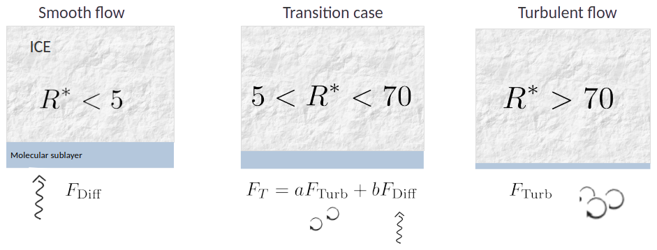
Figure 1 Conceptual representation of the parameterization developed which accounts for the nature of the flow under the ice (smooth vs turbulent) by weighting the contribution of molecular diffusivity and turbulent exchange in the transition case (for $\mathrm{5}<R{e}^{*}<\mathrm{70}$). The two weights a and b vary linearly between 0 and 1 as a function of the Reynolds number (Eqs. 5–6).

We developed a conceptual model that takes into account the different flow regimes i.e., smooth or turbulent, that can occur at the bottom of the ice, as well as the transition between the two (Fig. 1). The total flux F_T is then a weighted contribution of the two regimes:

$$\begin{array}{}\text{(3)}& F_{\mathrm{T}}=a{F}_{\mathrm{Diff}}+b{F}_{\mathrm{Turb}}.\end{array}$$

The two weights a and b are defined so that a=1 and b=0 in the full smooth regimes, and vice versa in the full turbulent regime. Between these two regimes, a and b decrease/increase linearly between 0 and 1. In order to define a and b, we used the roughness Reynolds number (Shirasawa and Ingram, 1991a) Re^*:

$$\begin{array}{}\text{(4)}& R{e}^{*}={\displaystyle \frac{h_{\mathrm{s}}{u}^{*}}{\mathit{\nu }}},\end{array}$$

where h_s is the mean height of the surface protrusions and ν is the kinematic viscosity ($\mathit{\nu }=\mathrm{2.1}\times {\mathrm{10}}^{-\mathrm{6}}$ m² s⁻¹). For computing the friction velocities we used a drag coefficient of $C_{\mathrm{d}}^{\mathrm{w}}=\mathrm{5.36}\times {\mathrm{10}}^{-\mathrm{3}}$ in both models following the standard approach of CICE + Icepack (Hunke et al., 2015). Previous studies (Nikuradse, 1933; Shirasawa and Ingram, 1991a) showed that the flow is hydraulically smooth for $R{e}^{*}<\mathrm{5}$ and hydraulically rough for $R{e}^{*}>\mathrm{70}$. In the case $\mathrm{5}<R{e}^{*}<\mathrm{70}$ the flow is in transition and is influenced by both viscosity and turbulence, thus the total flux of nutrients is given by Eq. (3) with the two weights assuming the form (see also the Supplement):

$$\begin{array}{}\text{(5)}& {\displaystyle }a& {\displaystyle }=\text{max}\left(\text{min}\left(\mathrm{1}-{\displaystyle \frac{\mathrm{1}}{\mathrm{65}}}\cdot \left(R{e}^{*}-\mathrm{5}\right),\mathrm{1}\right),\mathrm{0}\right)\text{(6)}& {\displaystyle }b& {\displaystyle }=\text{max}\left(\text{min}\left({\displaystyle \frac{\mathrm{1}}{\mathrm{65}}}\cdot \left(R{e}^{*}-\mathrm{5}\right),\mathrm{1}\right),\mathrm{0}\right).\end{array}$$

The mean height of the ice bottom protrusions h_s needs to be prescribed. The literature values vary between less than a millimeter to a few centimeters. Here, based on measurements by McPhee (2002, 2008) we used values between a minimum of $h_{\mathrm{s}}=\mathrm{0.6}\times {\mathrm{10}}^{-\mathrm{3}}$ m in the case of very smooth ice bottom, and a maximum of h_s=0.18 m, for a rough bottom. As described in Sect. 3 such values encompass the different flow regimes from fully smooth to fully turbulent.

2.2 Model description

We implemented and tested the Reynolds number parameterization in the Los Alamos (CICE + Icepack) (https://bb.cgd.ucar.edu/cesm/forums/cice-consortium.146/, last access: 26 May 2026) (e.g. Hunke et al., 2015; Jeffery et al., 2016) and in the new version of the SIMBA (Castellani et al., 2017) models. The former includes a vertically resolved biogeochemical setup, whereas the latter is based on bottom ice biogeochemistry.

2.2.1 CICE + Icepack

The Los Alamos Sea Ice Model includes two independent packages: CICE, for computing ice dynamic processes, and Icepack, that computes ice column physics and biogeochemistry. The model set-up used in the present study is described in Duarte (2025a) and Duarte (2025b) and available at the git repositories (https://github.com/pduarte8/CICE, last access: 27 May 2026, and https://github.com/pduarte8/Icepack, last access: 27 May 2026). As explained in Duarte et al. (2022), both CICE + Icepack are used together by defining a 1D vertically resolved model with 1 snow layer and 15 ice layers and 5×5 horizontal cells. Therefore, ice column physics and biogeochemistry are calculated by Icepack, but CICE is the model driver. The input file is the same as the one used in Duarte et al. (2022) and we refer to their Tables S1 and S2 for a list of the initial parameters used. The methodology for tuning the model parameters to better align with observational data is outlined in Sect. 2.5 and expanded in the Supplement.

We implemented Eqs. (2)–(6) in Icepack file icepack_brine.F90, in the subroutine compute_microS_mushy. This implied adding the parameters h_iceruf (h_s in Eq. 4) and alpha_s (α_s in Eq. 2) to the file icepack_parameters.F90.

2.2.2 SIMBA

We used a new version of the SIMBA model that was further developed from its first application in Castellani et al. (2017) and has a Git repository (https://github.com/EyringMLClimateGroup/Castellani2025_GMD_SIMBA2, last access: 27 May 2026) under Castellani (2025b). Version 2 of SIMBA includes two more limiting nutrients: silic acid and phosphate, besides the original nitrate. Another development is the transition from a fixed cell stoichiometry to a variable Chl a:C ratio as a function of nutrients concentration and light availability. This choice is particularly relevant for sea ice, where algae experience wide fluctuations of irradiance, in order to enhance the realism of the model (Ayata et al., 2013). In SIMBAv2.0, nutrients are exchanged at the sea-ice–ocean interface during ice growth and melt, through molecular diffusion, turbulence, and by the combination of processes described in Eq. (3). In the way it is coded, SIMBAv2.0 allows high flexibility; indeed, through several flags, it is possible to switch on and off the different terms for the resupply of nutrients. Similarly, the use of flags allows to select the limiting nutrient(s). The model equations and parameters used are presented in Appendix A.

SIMBAv2.0 is only a biogeochemical module so it needs the physics to be prescribed as forcing. In this study, we used the results for ice thickness from CICE + Icepack as input for SIMBAv2.0 for all three case studies. For snow thickness, we used observations taken at the coring site for the MOSAiC case study, whereas for the N-ICE2015 and Resolute case we used the CICE + Icepack output. Moreover, SIMBAv2.0 resolves only biogeochemical processes in the bottom of the ice. The thickness of the bottom layer can be chosen according to the resolution of the data used for comparison – in the present study, we set it to 10 cm for MOSAiC and N-ICE2015, and to 3 cm for Resolute. The initial choice of parameters reflected what was used in CICE + Icapack, further tuning is explained in Sect. 2.5 and in the Supplement.

2.3 Forcing data

We applied the new parameterization of nutrient exchanges at the ice–ocean interface to both models and tested them in three case studies (Fig. 2) – two from the Nansen Basin (Arctic Ocean), based on forcing data and ice floes monitored during the N-ICE2015 (Granskog et al., 2019) and the MOSAiC (Nicolaus et al., 2012; Shupe et al., 2022; Rabe et al., 2022) expeditions, and one from Resolute Bay in the Canadian Arctic (Mortenson et al., 2017). Data from the N-ICE2015 expedition and from Resolute Bay were detailed in previous modeling studies (Duarte et al., 2017, 2022; Mortenson et al., 2017). Therefore, here we briefly present only the MOSAIC data.

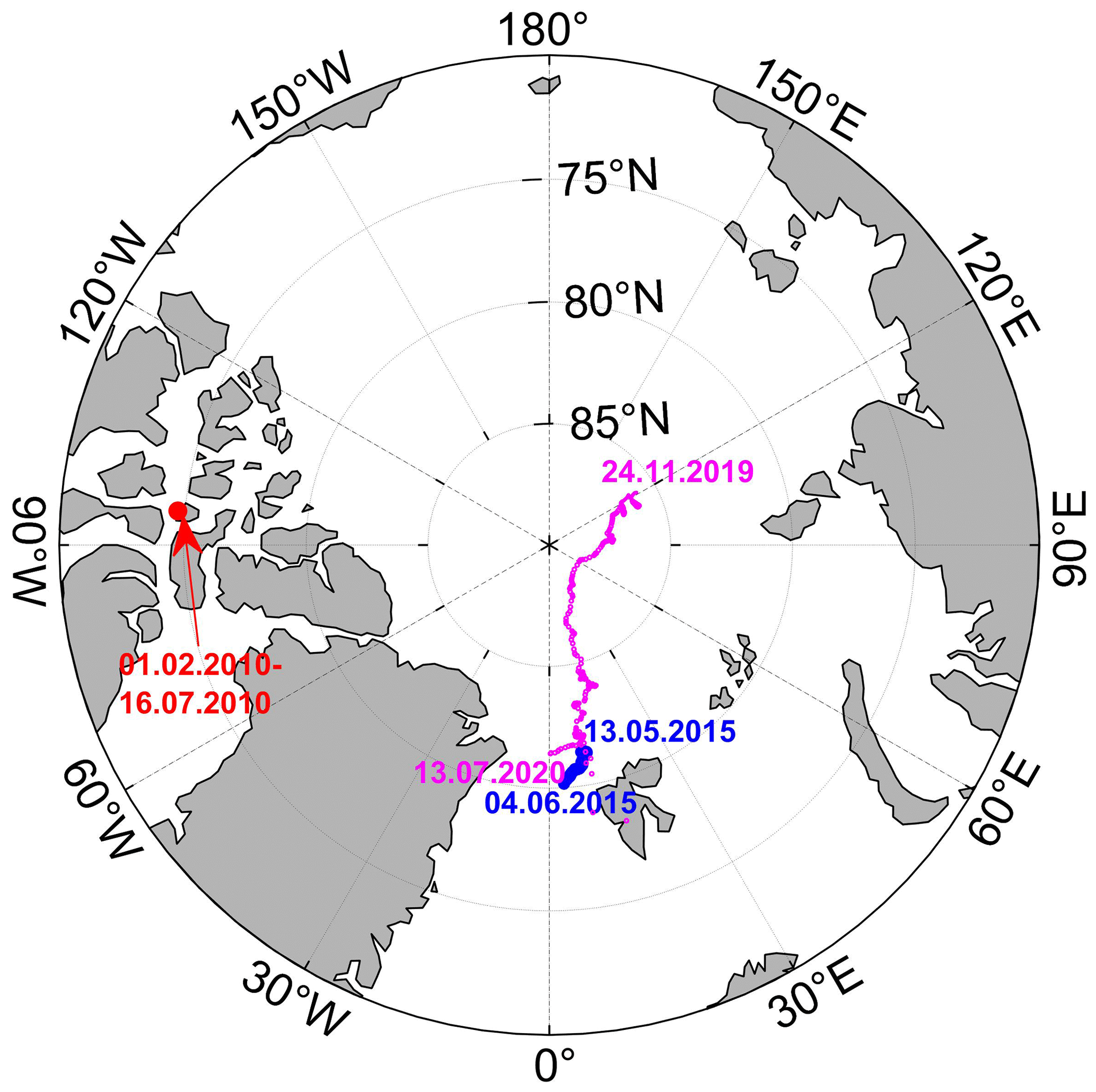
Figure 2 Map showing locations and time periods of the three data sets used for model comparison: MOSAiC – purple line, N-ICE2015 – blue line, and Resolute – Red dot.

The MOSAiC expedition took place from October 2019 to July 2020 with the aim of measuring a multitude of variables at a variety of spatial scales in the coupled atmosphere-ice-ocean system along the transpolar drift throughout a whole annual cycle. Expedition and data sampling are largely described in Shupe et al. (2022), Nicolaus et al. (2022), Rabe et al. (2022), and Fong et al. (2024), so we defer the reader to those references for a detailed description. The observational data collected during MOSAiC and used in this study to force the models are described in detail in Gu et al. (2024), here we will only provide a summary (see also Fig. 3). The atmospheric variables include: 6-hourly surface downward shortwave and longwave radiation, daily 2 m air temperature and specific humidity, 10 m wind speed, and precipitation. The oceanic data consist of daily 10 m sea temperature and salinity averaged from 8 CTD buoys, and 3 m sea temperature, salinity, and current velocity averaged from 4 autonomous ocean flux buoys. We forced the biogeochemistry module of CICE + Icepack and SIMBAv2.0 with observed nutrient concentrations in surface water (Torres-Valdés et al., 2024a, b, and Fig. 3f). Initial conditions for sea ice physical and biogeochemical variables are from ice coring data collected on 25 November 2019 (Oggier et al., 2024a, b; Hoppe et al., 2026). Observations of sea-ice draft and snow height from ice cores are shown in Fig. 3d, however we omitted a measurement taken at the end of March right after a rafting event (Angelopoulos et al., 2022), since with CICE + Icepack in the configuration used in the present study we can only simulate thermodynamic growth.

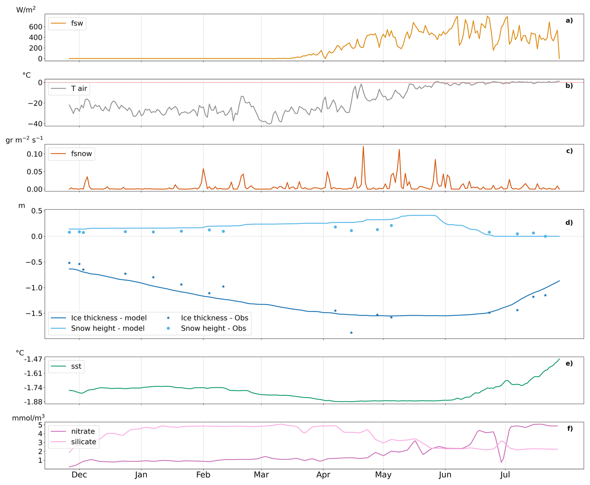
Figure 3 Overview of a subset of the forcing for the MOSAiC study case. Atmospheric forcing: (a) downward shortwave radiation (fsw), (b) 2 m atmospheric temperature (T_air), and (c) precipitation (fsnow). Panel (d) shows snow height and ice thickness as simulated by CICE + Icepack (line) together with observations collected during the coring events at the FYI site (dots/stars). Oceanic forcing: (e) sea surface temperature (sst), and (f) nutrients concentration in the water.

2.4 Model simulations

We compared the results of the runs performed with the new parameterization in which we varied the height of the bottom roughness protrusions h_s. The minimum value used is $h_{\mathrm{s}}=\mathrm{0.6}\times {\mathrm{10}}^{-\mathrm{3}}$ m, which corresponds to a fully molecular regime, and the maximum used is h_s=0.18 m, which corresponds to a fully turbulent regime (Sect. 3). The values in between are 0.0025, 0.005, and 0.01 m. In the MOSAiC case we performed simulations for the first-year ice (FYI). Table 1 lists the simulations performed and the main characteristics for each case study.

Table 1 Summary of simulations for the different case studies.

2.5 Tuning

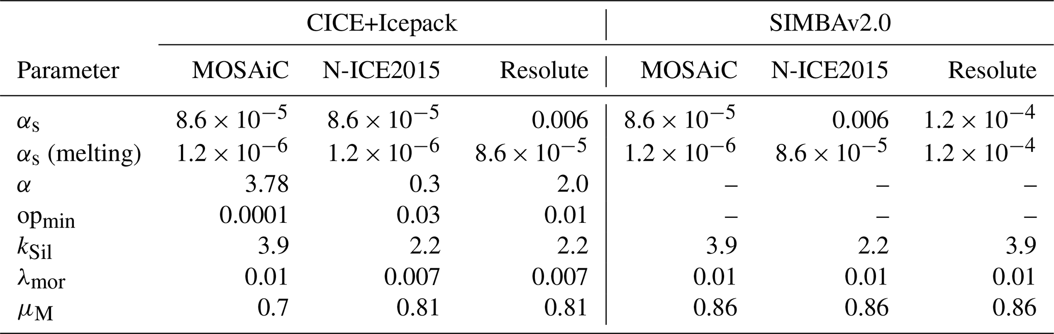
The CICE + Icepack configuration from Duarte et al. (2022) was originally tuned to represent the N-ICE2015 refrozen lead case. We used that set of parameters as initial control version of the model. The initial set of parameters for SIMBAv2.0 as used in Tedesco et al. (2026) has been modified to reflect what was used in CICE + Icepack. When simulating the MOSAiC case, however, CICE + Icepack model failed to represent the onset of algal growth. The reason lies in the fact that simulated snow height based on precipitation is larger than observations at the coring site (Fig. 3d) and algae remain light limited until the end of May (onset of surface melt). We thus tuned the light limitation parameter α of the CICE + Icepack model to match observations. Details of the tuning are presented in the Supplement, the tuned parameters are presented in Table 2. We aimed at keeping the values of parameters the same in both SIMBAv2.0 and CICE + Icepack, however this has not been possible due to intrinsic differences between the models. For example, to better reproduce the N-ICE2015 case with SIMBAv2.0 we had to increase the exchange coefficient α_s (see Table 2) and we had to allow algae to stick to the ice bottom (i.e., to not be released during melting). This tuning approach has already been discussed for the same case study with different models in Tedesco et al. (2026). In the Resolute case, for both SIMBAv2.0 and CICE + Icepack we used a larger value of the exchange coefficient α_s compared to the MOSAiC case to allow accumulation of biomass to the levels observed. For all case studies, we kept the exchange coefficient constant during the simulation period, but we accounted for stratification by lowering its values by ∼ 1 order of magnitude in the case of bottom melt following McPhee (2008). It has to be noted that the aim of this study is to test the sensitivity of the models in reproducing algal phenology to the parameterization of fluxes at the ocean-ice interface, so an in-depth tuning of the models to represent the different case studies is beyond the scope of this manuscript.

Table 2 Values of tuned parameters for CICE+Icepack and SIMBAv2.0. α_s is the exchange coefficient in Eq. (2), adimensional; α (m² W⁻¹) and op_min (adimensional) are parameters used to calculate light limitation in Icepack (Jeffery et al., 2016); k_Sil (mmol m⁻³) is the half saturation constant for silicate; λ_mor is the mortality rate (d⁻¹); μ_M is the maximum growth rate (d⁻¹). Note that SIMBAv2.0 calculates light limitation differently so it does not use the same α and op_min as Icepack.

3 Results

3.1 MOSAiC case study

The friction velocity u^* ranged between nearly zero and 0.02 m s⁻¹ (Fig. 4a). Although the Reynolds number Re^* correlated with u^*, its magnitude was largely dependent on h_s (Fig. 4b). With 0.0025 $\le h_{\mathrm{s}}\le$ 0.01 m, Re^* remained between 5 and 70, implying that the flow regime was in transition between smooth (viscosity-dominated) and turbulent. Therefore, both molecular diffusion and turbulence contributed to the nutrient fluxes. In the case of the lowest h_s (=0.6 × 10⁻³ m), Re^* was always <5, implying that the flow was smooth and nutrient exchanges were driven only by molecular diffusion. For the largest h_s value (=0.18 m), the Reynolds number was always above 70, so the fluxes were entirely driven by turbulence (Sect. 2.1).

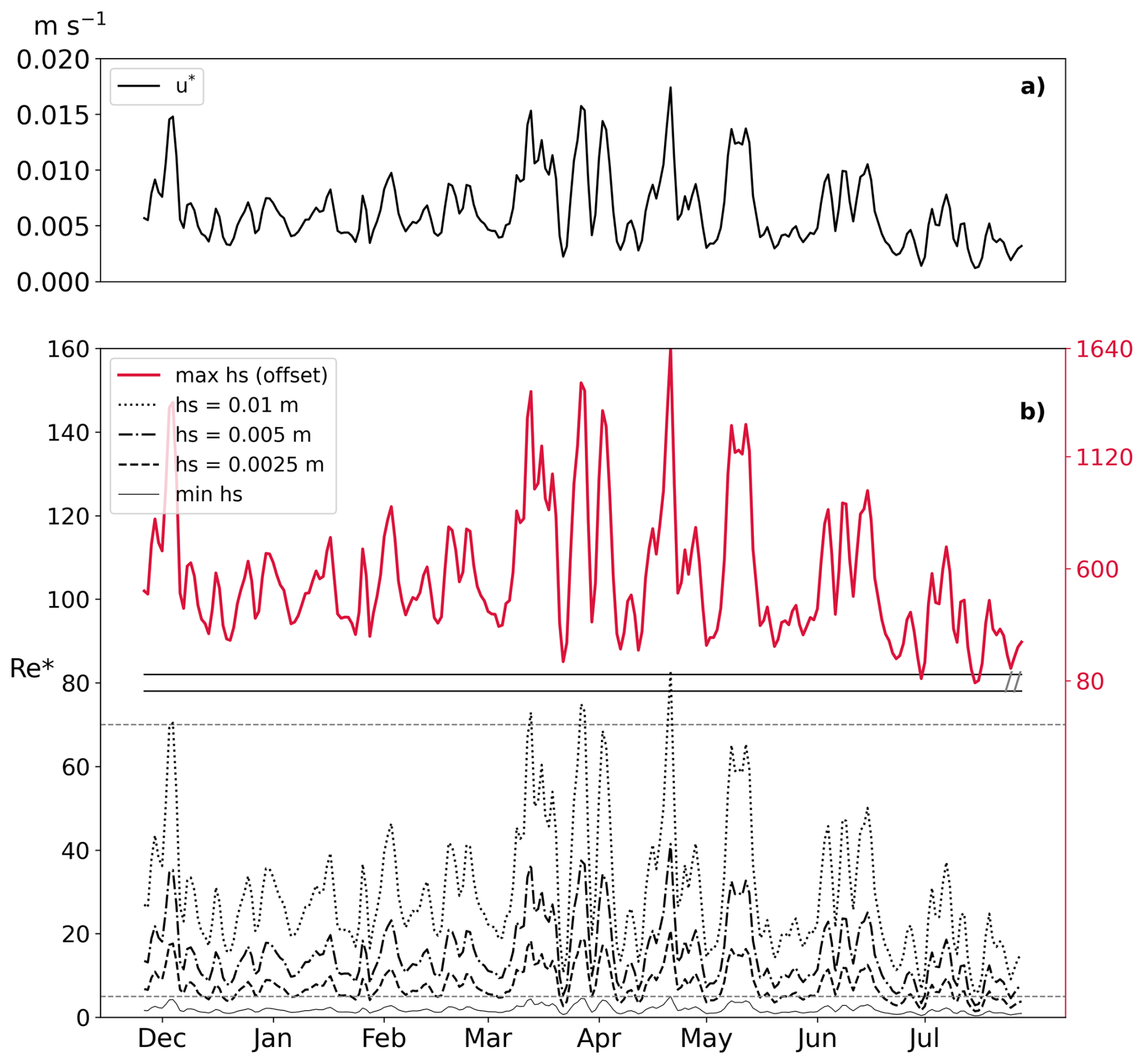
Figure 4 MOSAiC case study: (a) Friction velocity; (b) roughness Reynolds number Re^* for all the different sizes of roughness elements tested. The horizontal dashed lines at $R{e}^{*}=\mathrm{5}$ and $R{e}^{*}=\mathrm{70}$ depict the upper limit for a smooth flow and the lower limit for a rough turbulent flow, respectively. Note that the values of Re^* for the maximum roughness (red colour) are represented on a different scale (y-axis on the right side).

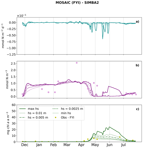
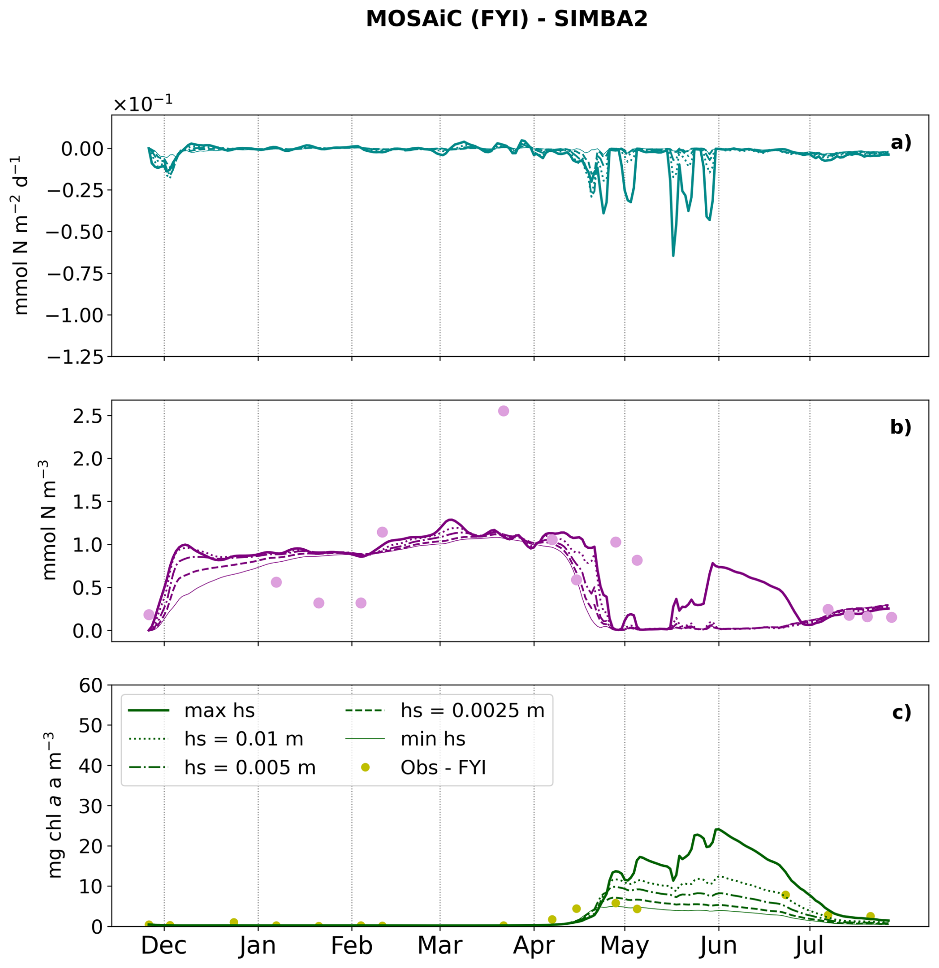
Our analysis will focus on nitrate, the primary nitrogen source for the spring bloom, and silicic acid (reported in the Supplement) to compare nutrient concentrations and fluxes across different simulations. The fluxes of nitrate at the ice-ocean interface were predominantly negative (from the ocean to the ice) and of the same order of magnitude using either CICE + Icepack or SIMBAv2.0 (Figs. 5a, 6a respectively). However, their value was slightly larger in the former model. The larger negative values occurred in spring-summer, precisely in April (in the case of CICE + Icepack) and May (SIMBAv2.0). The variability of fluxes preceding the spring period (before April) was relatively low. Fluxes increased with increasing h_s in both models. For very smooth ice, fluxes were nearly zero, but rose to approx. −1.25 × 10⁻¹ mmol m⁻² d⁻¹ in CICE +Icepack (and to approx. −0.75 × 10⁻¹ mmol m⁻² d⁻¹ in SIMBAv2.0) when the roughness increased to the maximum value tested. At the beginning of the simulation period (November–December) the gradient of nitrate between the sea-ice bottom and the ocean caused larger fluxes than during the rest of the winter. Fluxes of silicic acid are presented in the Supplement (Fig. S1).

Both models showed an initial increase in bulk nitrate concentration in the ice bottom (Figs. 5b and 6b). We note here that CICE + Icepack resolves biogeochemistry in 15 layers within the ice column. Thus, in order to select the bottom 10 cm we applied a weighted average of the number and portion of layers that are included in this depth range. In CICE + Icepack, concentrations stabilized around 0.5 mmol m⁻³ and showed no trend during winter. In SIMBAv2.0 the concentration of nitrate stabilized at values around 1.0 mmol m⁻³, and showed no or very little increase during winter. In both models, the bottom of the ice became depleted in nitrate in April–May. The depletion of nitrate corresponded with the co-occurring ice algal blooms (Figs. 5c and 6c). Compared with observations, CICE + Icepack exhibited bottom nutrient values lower than those measured (Fig. 5b), whereas SIMBAv2.0 showed larger values (Fig. 6b). Both models failed to capture the full variability observed, which may partly reflect spatial heterogeneity in the ice core data. In both models, when the ice was smooth (min h_s), the nitrate concentration began to decrease earlier, with the bottom of the ice completely nitrate-depleted earlier than in other cases, thus preventing further algal growth. In all other cases of bottom roughness, nutrients were depleted by early May. When turbulence was included (i.e., for all values of h_s above minimum), nutrient concentrations began to increase again after the peak of the algal bloom. Ice algal biomass is presented as chlorophyll a (chl a) concentration. In CICE + Icepack biomass is calculated in nitrate units, so we followed Duarte et al. (2017) and applied a conversion factor of 2.1 mg chl a mmol N⁻¹ (Smith et al., 1993). Differently, SIMBAv2.0 has a variable Chl a:C, and thus Chla:N, ratios so chl a content was computed at each time step. The time series of Chl a:C is shown in the Supplement. Chl a remained close to zero until spring and reached its maximum in June in both models. However, differences in algal phenology can be seen between the different values of the roughness parameters: Algal biomass reached a plateau in both models that remained approximately stable in May in all simulations, except the one with the fully turbulent case (h_s=0.18 m) where algae kept growing until a maximum. CICE + Icepack predicted larger ice algal biomass with a maximum about three times that in SIMBAv2.0. This is due to the tuning of the photophysiology parameter in CICE + Icepack: a larger light limitation factor α pushed algal bloom earlier in the season to match observations, but it also led to larger biomass accumulation. It has to be noted that observational data for chla a are unavailable from early May to late June – coinciding with the development of the spring algal bloom – making direct comparison between model and observations difficult. However, the model correctly simulated the onset of growth and captured the maximum in June, indicating the potential for a robust representation of algal phenology. The case that better matches the few observations available is the one with the lowest values of bottom roughness (when molecular exchanges dominate) for both models.

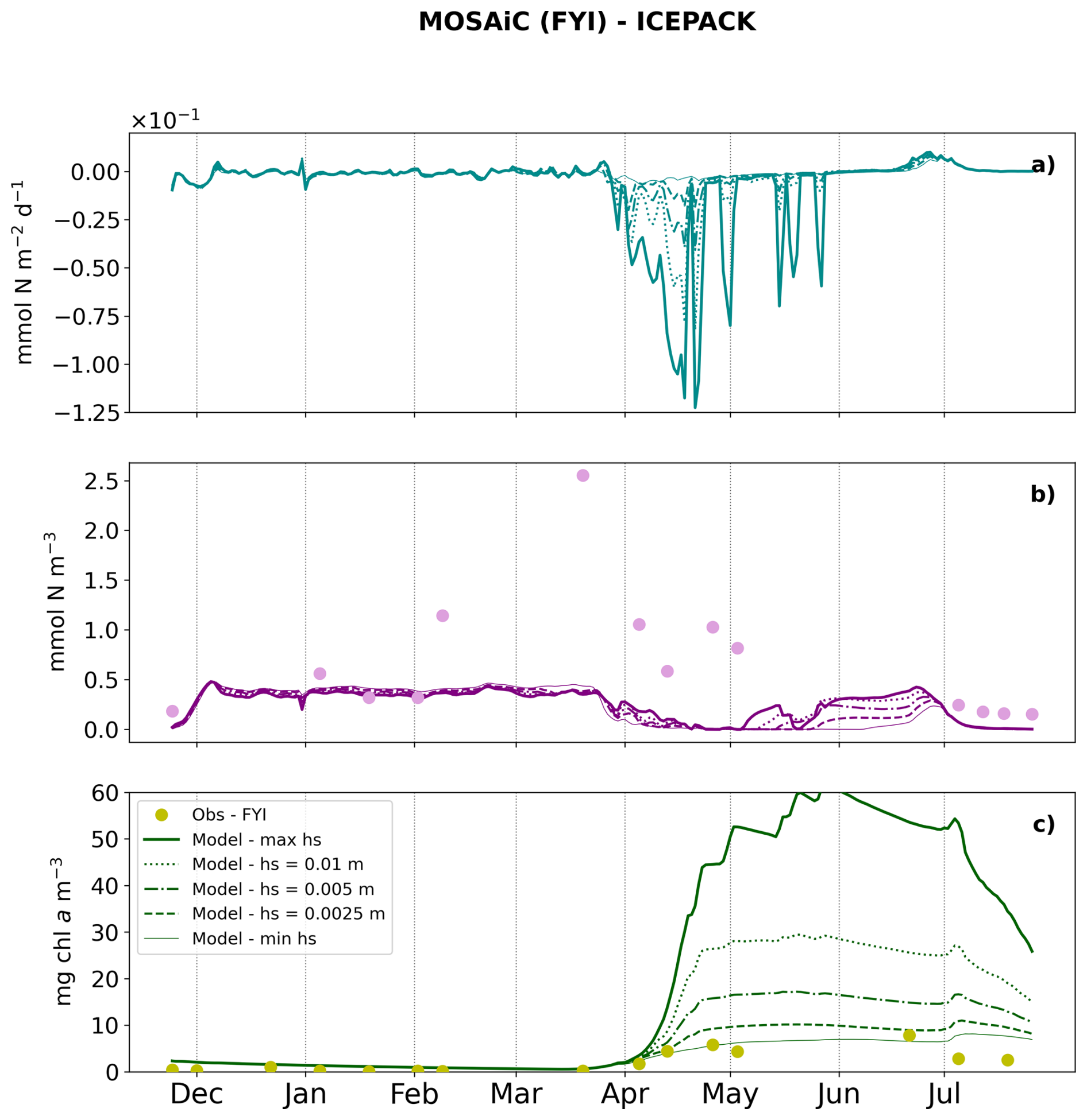
Figure 5 MOSAiC case study: CICE + Icepack results for all tested sea-ice roughness values: (a) Nitrate fluxes at the ice-ocean interface (negative when directed from the ocean to the ice); (b, c) Nitrate and chl a concentration in the sea ice bottom 10 cm, respectively. Dots represent observations from ice cores collected on FYI (Hoppe et al., 2026).

Figure 6 Same as Fig. 5 but for SIMBAv2.0 results.

In CICE + Icepack the bulk concentration of nitrate was larger in the bottom than in the ice interior (Fig. 7, lower row) for all values of h_s. In the case of smooth ice, the decrease in nutrient concentration seen at the end of March and beginning of April in the sea ice bottom (Fig. 5b) extended up to 50 cm in the ice column. For rougher ice, the concentration of nutrients recovered to its pre-bloom values in mid June in the bottom 25 cm of the sea ice. At the end of the simulations, nutrients were depleted from the entire ice column in all cases, coinciding with flushing of melted snow through the ice. Algae remained mostly concentrated at the ice bottom in all simulated cases.

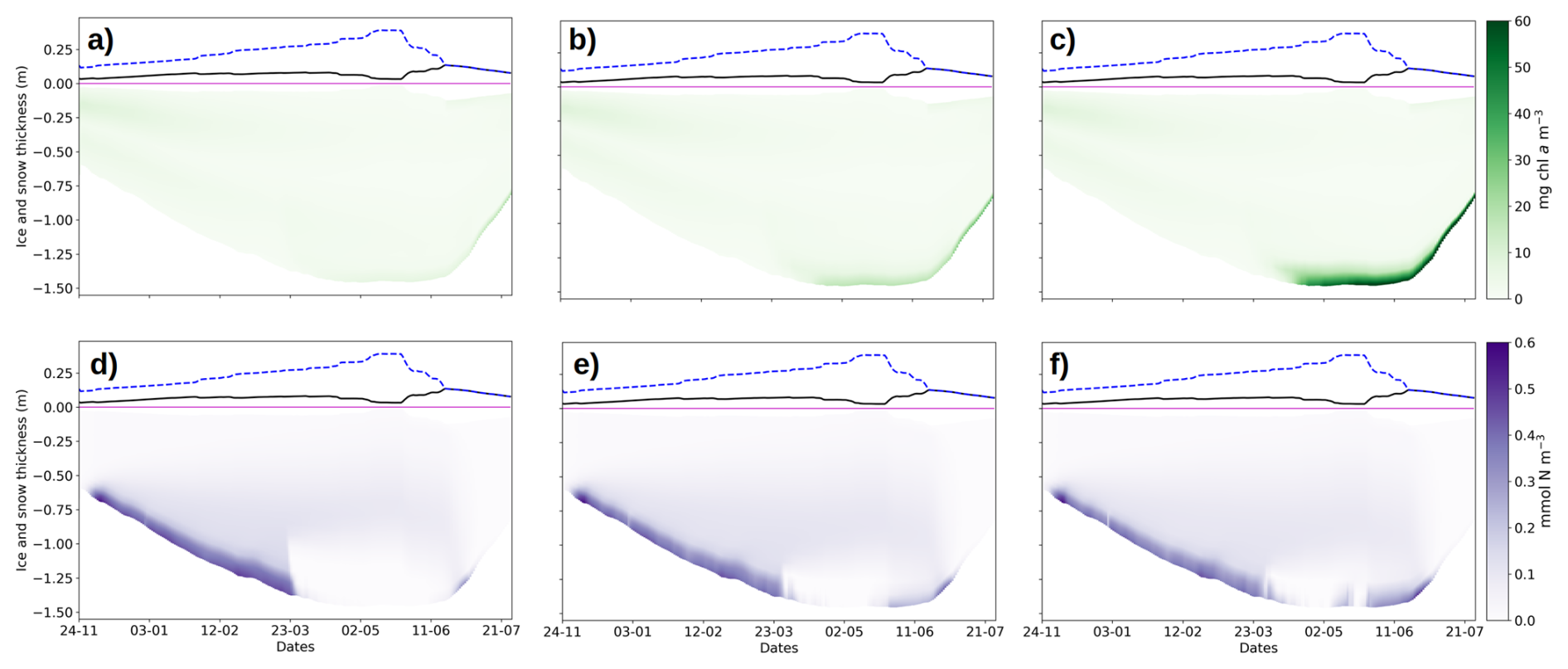
Figure 7 MOSAiC case study: Vertically resolved chl a and bulk nitrate concentration (top row and lower row, respectively) in CICE + Icepack in the case of (a–d) minimum h_s; (b–e) h_s=0.005 m; (c–f) maximum h_s. The blue dashed and the black lines represent snow height and freeboard, relative to the sea level (magenta line) as simulated by the model.

3.2 N-ICE2015 case study

The results presented here are from a refrozen lead detailed in previous studies and reaching a maximum ice thickness and snow height of ∼ 30 cm and a few millimeters, respectively (Duarte et al., 2017, 2022). The refrozen lead was monitored regularly between its formation on the 24 April until the beginning of June 2015. Friction velocities were in the same range of the MOSAiC case (0.0–0.02 m s⁻¹), but with fewer values exceeding 0.01 m s⁻¹ (Fig. 8a). Also in this case the flow was smooth under the smallest h_s, while for maximum roughness the flow was fully turbulent. For the values in between, the flow was in transition (Fig. 8b). Algal biomass followed the same pattern observed in the MOSAiC case for both models: greater sea-ice roughness led to increased algal growth (Fig. 9). The two models accumulated a comparable algal biomass and showed improved agreement with observations compared to the MOSAiC case. It should be noted, however, that CICE + Icepack was previously tuned using this dataset (Duarte et al., 2017) when only molecular diffusivity was implemented, therefore, it is not surprising that it reproduced observations more accurately in the N-ICE2015 case. The former version of SIMBAv2.0 was also tuned on this data set (Tedesco et al., 2026), but in its new model configuration SIMBAv2.0 was able to reproduce observations only when turbulence was considered.

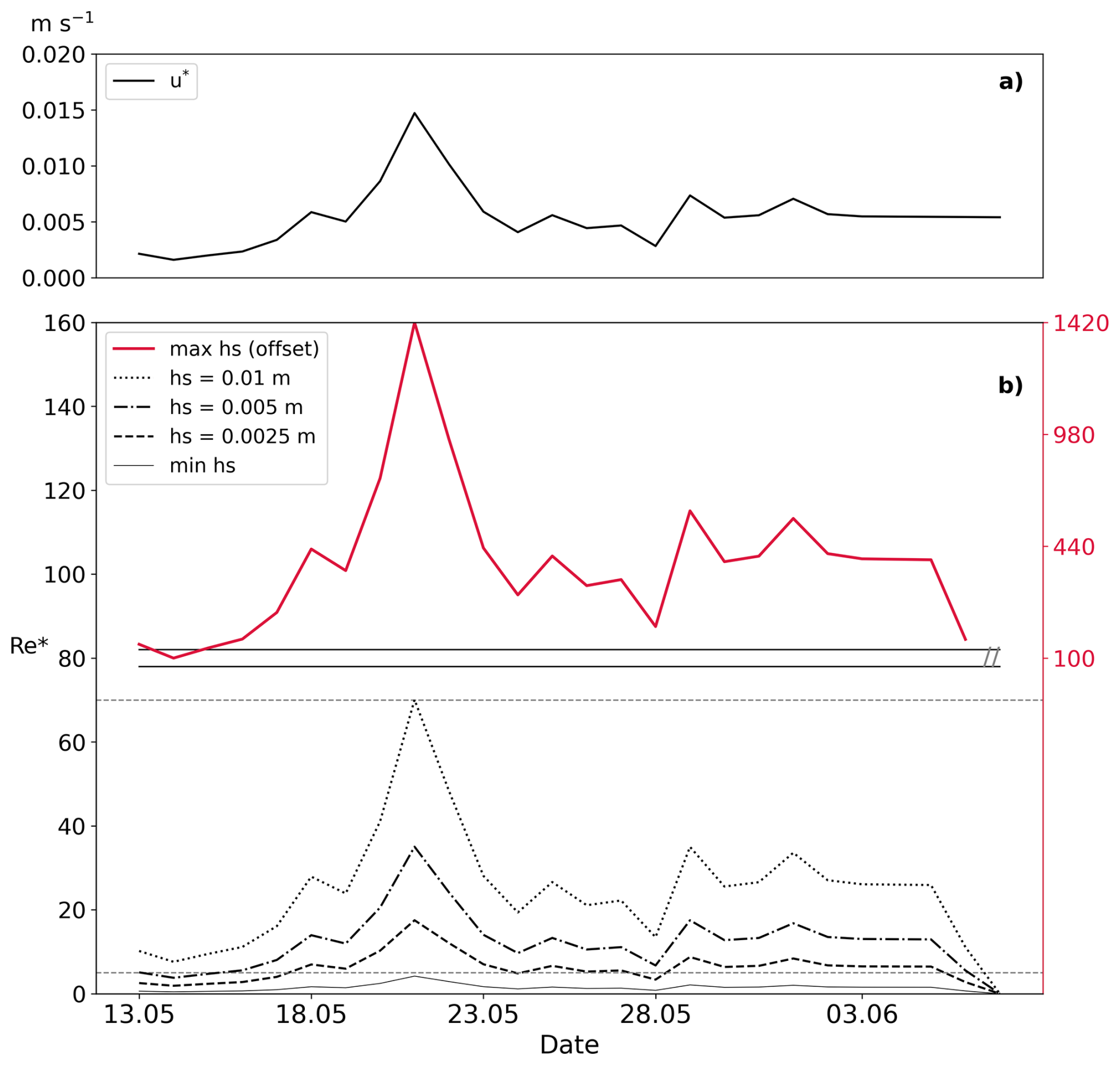
Figure 8 N-ICE2015 case study: (a) Friction velocity; (b) roughness Reynolds number Re^* for all the different sizes of roughness elements tested. The horizontal dashed lines at $R{e}^{*}=\mathrm{5}$ and $R{e}^{*}=\mathrm{70}$ depict the upper limit for a smooth flow and the lower limit for a rough turbulent flow, respectively. Note that the values of Re^* for the maximum roughness (red colour) are represented on a different scale (y-axis on the right side).

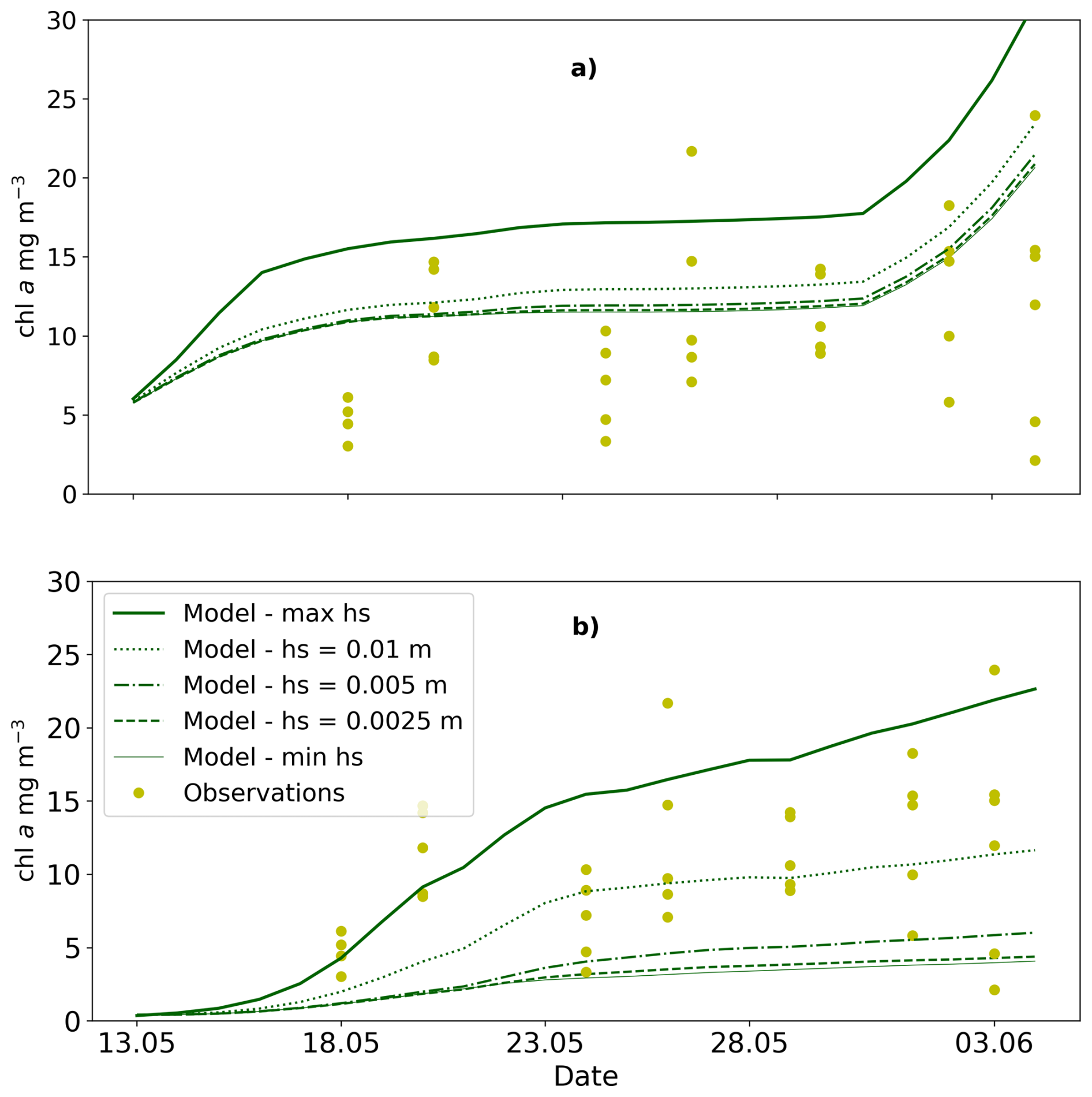
Figure 9 N-ICE2015 case study: Chl a concentrations in the sea-ice bottom 10 cm in (a) CICE + Icepack, and (b) SIMBAv2.0.

3.3 Resolute case study

Friction velocity remained always below 0.01 m s⁻¹ during the Resolute time series (Fig. 10a). For most of the roughness values above the minimum, however, the flow remained in transition between smooth and turbulent, despite the low Reynolds numbers ($R{e}^{*}<\mathrm{40}$). For the maximum roughness, the Reynolds number was above the limit for turbulent flow (Fig. 10b). For consistency with the depth range of the observations (Mortenson et al., 2017) we present average chl a concentrations for the bottom 3 cm (Fig. 11). Observed values in the sea-ice bottom were two orders of magnitude larger than those of the previous case studies. Both models predicted chl a concentrations proportional to h_s and were able to reach observed values only when turbulence was considered. Irrespective of the h_s chosen, the CICE + Icepack model predicted strong nitrate depletion (Fig. 12) that extends through the entire ice column. For roughness values above the minimum, the ice bottom was replenished with nutrients during algal growth, but the ice interior remained depleted, apart for a small amount of nutrients at the surface when snow melted around 20 June.

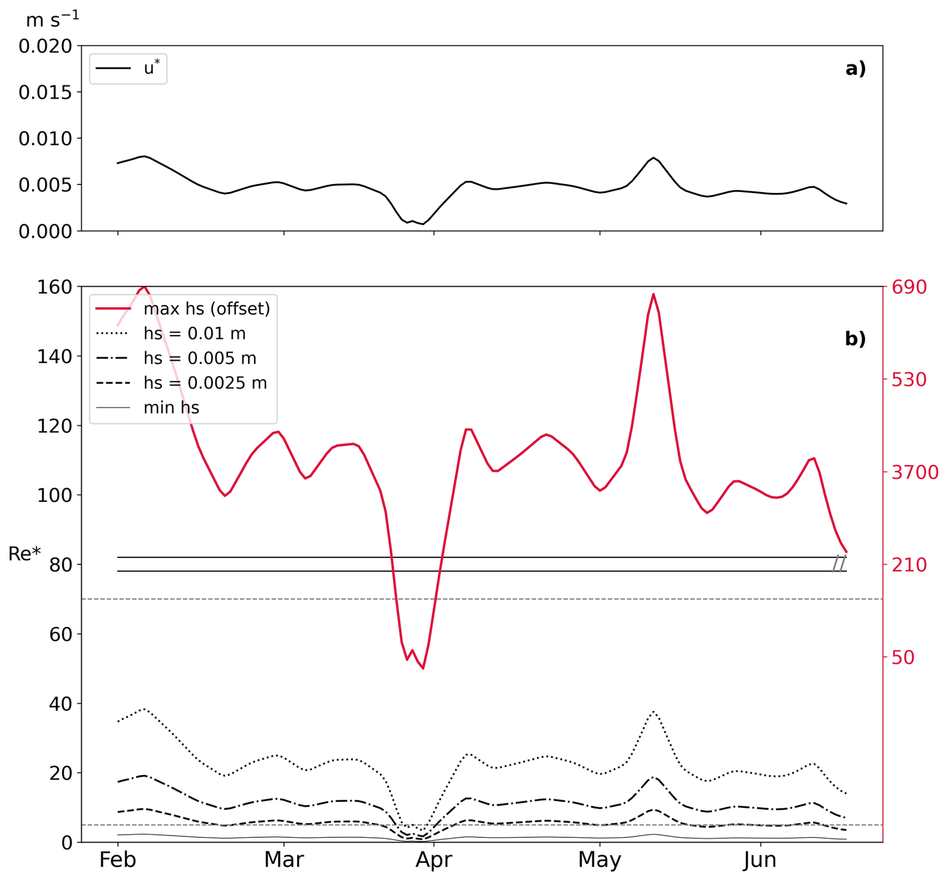
Figure 10 Resolute case study: (a) Friction velocity; (b) roughness Reynolds number Re^* for all the different sizes of roughness elements tested. The horizontal dashed lines at Re^*= 5 and $R{e}^{*}=\mathrm{70}$ depict the upper limit for a smooth flow and the lower limit for a rough turbulent flow, respectively. Note that the values of Re^* for the maximum roughness (red colour) are represented on a different scale (y-axis on the right side).

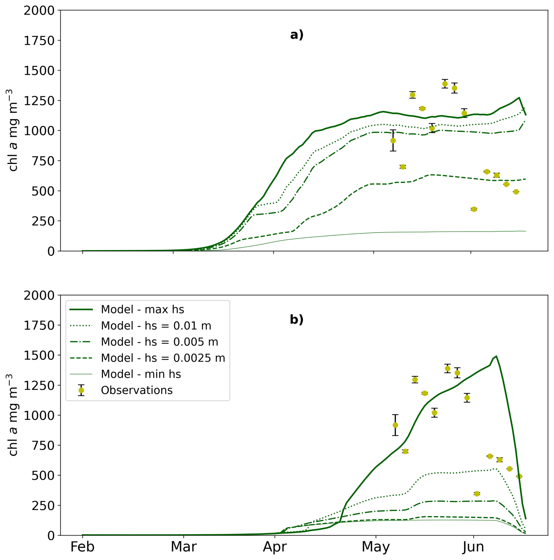
Figure 11 Resolute case study: Chl a concentrations in the sea-ice bottom 3 cm in (a) CICE + Icepack, and (b) SIMBAv2.0.

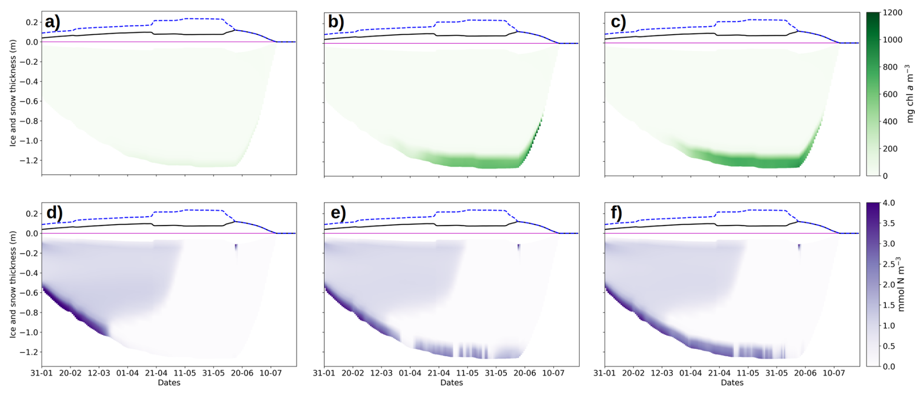
Figure 12 Resolute case study: Vertically resolved chl a and nitrate concentration (top row and lower rows, respectively) in CICE + Icepack in the case of (a–d) minimum h_s; (b–e) h_s=0.005 m; (c–f) maximum h_s. The blue dashed and the black lines represent snow height and freeboard, relative to the sea level (magenta line).

4 Discussion

4.1 Parameterization of Ocean Fluxes

The physics governing the fluxes of nutrients at the ice-ocean interface happen at small scales that are not resolved by current sea-ice models. The mixing and exchange processes therefore need to be parameterized. Based on boundary layer and eddy-covariance studies, the flow at the ice-ocean interface that determines such exchanges can be smooth or turbulent, leading to molecular diffusion or turbulent driven exchanges, respectively (e.g., McPhee, 2008; Long et al., 2012). Many sea-ice biogeochemical models include one of these exchange types, with a preference for the former. However, fluxes due to molecular diffusion (dominated by viscosity) are often too small to provide enough nutrients to explain the biomass accumulation observed in the field (Dalman et al., 2019; Van der Linden et al., 2020; Roukaerts et al., 2021). This may be the reason why Lavoie et al. (2005) used a formulation based on molecular diffusion where the thickness of the boundary layer is calculated as a function of friction velocity. Similarly, Jin et al. (2006) used a diffusion coefficient 4 orders of magnitude higher than the molecular diffusivity, and Watanabe et al. (2015) assumed that ice algae may uptake nutrients directly from seawater, based on a study by Boetius et al. (2013). However, this last study was focused on Melosira arctica, which forms aggregates or macroscopic strand colonies at the bottom-ice interface, whereas our focus is on the more common occurrence of ice algae living within the brine network and skeletal layer. Very few models parameterize the exchange fluxes as turbulent (e.g. Haddon et al., 2024), and none include the contribution of both viscosity and turbulence dominated regimes. In the present study, we developed and implemented a new parameterization that accounts for the contribution of the two regimes, allowing the flow to be in a transitional stage between smooth and turbulent. The fluxes are thus the result of a weighted contribution of both processes.

In our three case studies, we found that the friction velocity was in the range of previous observations (e.g., McPhee, 2008). Furthermore, we found that the friction velocity was generally high enough to keep the flow in a transition between smooth and turbulent. With low current velocity and, thus, low friction velocity, viscous forces gain importance and the thickness of the molecular sublayer limits the exchange fluxes. This was shown by Long et al. (2012) during an eddy-covariance study in a southwest Greenland fjord, where stratification and low current velocities prevented the determination of oxygen fluxes during more than half of the instrument deployment time. In addition to velocity, the flow regime is also determined by the roughness of the ice bottom. It is indeed the ratio between the thickness of the molecular sublayer (function of u^*) and the height of the roughness elements h_s that determines the nature of the flow (Nikuradse, 1933; Shirasawa and Ingram, 1991a, b; Kadivar et al., 2021). When roughness elements at the ice-ocean interface are larger than the thickness of the molecular sublayer the flow may shift from smooth to rough (see Supplement of Olsen et al., 2019, and references therein). This thickness of the molecular sublayer δz can be estimated with (Lavoie et al., 2005, and references therein):

$$\begin{array}{}\text{(7)}& \mathit{\delta }z={\displaystyle \frac{\mathit{\nu }}{u^{*}}}.\end{array}$$

For friction velocities in the range of the MOSAiC case study, the thickness of the molecular sublayer ranges between a maximum of 2 mm and a minimum of 0.1 mm. In Lavoie et al. (2005) the thickness of this sublayer was <1 mm. The bottom roughness in multiyear ice during the SHEBA experiment was 0.0048–0.007 m, i.e. around 6 mm (McPhee, 2002) and larger than our estimates of δz. We do not have information on the small scale roughness of the ice bottom in our three case studies, thus we tested different values covering the literature range. The range of variability of the thickness of the molecular sublayer and that of the bottom roughness suggests that the flow under the sea ice may easily shift from smooth to turbulent, since the latter is larger than the former. The dependence on sea-ice roughness is a limitation of the current parameterization, since roughness measurements are usually not conducted during sea-ice monitoring. Moreover, it should be noted that the Reynolds number depends on the value of the oceanic drag coefficient through the friction velocity. We could have changed the value of the drag coefficient, which itself is a measure of bottom roughness, rather than the roughness parameter directly. However, the drag coefficient in CICE + Icepack is also used in the momentum equation, thus we would have introduced other effects difficult to disentangle in our analysis. When considering large scale applications, a simple approach would be to rely on a fixed value of h_s in the middle range of those tested in the present study. Another approach could be based on the determination of the value of such parameter based on ice type/age. For those models that include deformation processes, values of bottom roughness could be based on the amount of deformation per grid cell (e.g., Castellani et al., 2018). However, the scale of deformation may not be relevant for the scale of the molecular sublayer and targeted observations are needed to better relate nutrient fluxes to ice deformation.

In the MOSAiC case, our parameterization led to a simulated increase in ocean-ice nutrient fluxes that was proportional to roughness. The concentration of nutrients in the ice bottom did not vary substantially for most of the study, but large changes occurred as soon as algal growth began, after release from light limitation. The two models showed different equilibrium concentrations with SIMBAv2.0 showing higher concentration in the bottom ice. Differences between the two models can be explained by discetization and complexity, indeed SIMBAv2.0 does not compute brine fraction but it uses a fixed value for the skeletal layer, whereas Icepack calculates brine fraction in each layer based on thermodynamic processes. Differences in brine fraction between the models would lead to differences in bulk concentrations. Both models, though, agreed with observations (panel (b) in Figs. 5 and 6), since the latter are scattered around 0.5 and 1.0 mmol N m⁻³, except for one large value at the end of March. This “outlier” may be attributed to a rafting event (Angelopoulos et al., 2022), and it is thus of a dynamic nature (unresolved by our models). In July, observed values are lower and simulations with both models agreed well. In both models nutrients flushed into the ice were then transferred upwards. However, the two models are very different in nature (i.e., CICE + Icepack is vertically resolved and calculates brine convection, whereas SIMBAv2.0 has only bottom algae and the transport of nutrients upwards is only due to remapping during ice growth/melt). The trend in nutrients is visible in the vertically integrated time series for Icepack (shown in the Supplement) and in the concentration of nutrients in the upper layer of the ice in SIMBAv2.0. It has to be noted that in SIMBAv2.0 the nutrients are simply stored in the above layer and are not used for any biological production.

4.2 Algal Phenology

In the MOSAiC case, modelled algal bloom started in April. Algal growth led to an increase in nutrient fluxes, especially in CICE + Icepack case. This increase in nutrient fluxes did not lead to larger accumulation of nutrients in the ice bottom, but nutrients were rather utilized immediately by algae to sustain the growth. The higher the bottom roughness parameter (thus, the higher the turbulence), the more algae could grow in both models. In SIMBAv2.0 the maximum biomass accumulated in the case of fully turbulent flux was almost four times larger than in the case of molecular diffusion, and it was even larger for CICE + Icepack. Initiation of growth, as well as timing of maximum biomass were not affected by the nature of the exchanges, but rather by light limitation. SIMBAv2.0 was forced with snow observations collected at the coring site and was able to represent the algal increase in April without tuning. In CICE + Icepack we had to tune the value of the light limitation factors to match observations (see Supplement). The reason for such tuning is that, based on precipitations, the model predicted thicker snow cover on the order of 25 cm (Fig. 7) at the time of the observed algal growth. Such thick snow cover prevented the initiation of the bloom. It should however be noted that this early growth in observations was unexpected (Hoppe et al., 2024) and probably due to very efficient light use from sea-ice algae. Thus, it is no surprise that a tuning of the light limitation parameter was needed in the model to represent such early growth. Between the beginning of May and mid July, no observations are available (Fong et al., 2024), thus it is not possible to know what was the maximum biomass accumulated during that time. Maximum biomass was reached at the same time for all different roughness values, and in both models it occured at the end of May. Models represented better observations in the case of molecular diffusivity only. The explanation could reside in two possible mechanisms: it is possible that the ice bottom was so smooth to not develop any turbulent exchange. On the other hand, during MOSAiC a freshwater layer was observed (Smith et al., 2022, 2025) that accumulated under the ice. Such layer was isolating the bottom of the ice from the more nutrients-rich sea water, thus impeding nutrients resupply to the ocean-ice interface. This points to the large complexity of both collecting measurements (nutrient concentrations in water should be measured close to the ice bottom) and modeling sea-ice physical and biogeochemical processes to represent observations.

In the MOSAiC case, observations are sporadic so it is difficult to constrain model results. However, both in the N-ICE2015 and Resolute cases observations are available at higher time resolution. In the N-ICE2015 case, both models agreed with observations for at least 2–3 values of bottom roughness considered. Both models simulated algal biomass accumulation, which was recorded in the refrozen lead. It has to be noted that CICE + Icepack was tuned (Duarte et al., 2017) to simulate the refrozen lead case before the parameterization was introduced, and when only molecular diffusion was considered (the default process in Icepack biogeochemistry). This explains why the case of minimum sea-ice roughness was able to capture the right accumulation of biomass. It should also be noted that the tuning carried out in Duarte et al. (2017) was independent of the flux parameterization. Specifically, Duarte et al. (2017) reduced the half-saturation constant for silicate uptake by almost 50 %. While this adjustment affects ice-algal physiology and illustrates how tuning can be used to compensate for the absence of a more physically based representation of the system, such tuning may also reduce the model’s realism by shifting physiological parameters away from observed or experimentally derived values. In SIMBAv2.0 the observed algal accumulation was properly simulated only when the contribution of turbulence was taken into account. Resolute is a particular case characterized by very large biomass accumulation (Mortenson et al., 2017). Here, both models accumulated larger biomass compared to the other two cases, mainly due to the larger ocean nutrient concentrations than in the previous case studies. Both models were able to reproduce observations only when the contribution of turbulence was taken into account. This shows the potential importance of turbulence in sustaining growth and in representing algal accumulation without relying on tuning parameters that are not well constrained by observations. For CICE + Icepack we also had to increase the light limitation parameter α (Table 2). The 1D model intercomparison of Tedesco et al. (2026) showed that the parameters that are often tuned to match observations are the half saturation constants and the maximum chl-specific growth rate. Although such tuning strategies allow better representation of observed phenology, they still fail in representing nutrient concentrations in the ice. The model intercomparison of Tedesco et al. (2026) was focusing on Arctic data, however recently Lim et al. (2019) tuned the half saturation constant for silic acid in order to match a 17 d time series of biogeochemical sea-ice observations from Davis in East Antarctica.

The response of the two models to the new parameterization was consistent: turbulence enhanced the nutrient fluxes at the ice-ocean interface. This led to a reduction in nutrient limitation and a significant increase in chl a biomass accumulation in the ice, particularly in the bottom-ice. The parameterization performance was comparable in the two models presented in this study, so it may be used in models with different complexity. The fluxes have no influence on the onset of the bloom, which is determined by light availability. In the MOSAiC case, we had to increase the light limitation parameter in CICE + Icepack to reproduce the observed algal growth, even though the model still indicated thick snow cover. This suggests a fundamental limitation in the current modeling framework: while the model simulates snow accumulation based on precipitation and standard thermodynamic physics, it may not accurately represent the true snow height or distribution – particularly in regions where local processes such as wind-driven snow redistribution, rafting, or ridging events significantly alter the snow cover. These sub-grid-scale processes, which are not captured in a one-dimensional (1D) model, can lead to localized thinning of snow and enhanced light availability, thereby enabling algal growth despite seemingly unfavorable conditions. Thus, the need to adjust the light limitation parameter may reflect a symptom of missing physical realism in the snow–ice–light coupling rather than a real need for biological tuning, thus underscoring the importance of incorporating higher-resolution or process-based representations of snow dynamics in future model developments. On the other hand, algal physiology may be such that in reality algae can start growing at very low light levels (Hoppe et al., 2024) but the model is not able to represent such physiological trait, suggesting that a variable photosynthetic efficiency α could be more appropriate than one constant value. In contrast, SIMBAv2.0 offers a more practical alternative for process evaluation and model–observation comparison, as it does not simulate the underlying physical processes (e.g., snow accumulation, ice growth, or brine dynamics) but instead relies on prescribed ice and snow thicknesses. This allows the model to be directly forced by observations, making it easier to isolate and evaluate biogeochemical responses. Despite the fact that SIMBAv2.0 is only a biogeochemical model, so it does not resolve physics, the main differences between the two models lie in the complexity of the biological processes. For example, CICE + Icepack includes ammonia; a temperature dependent description of mortality; a zooplankton term; a different parameterization of light limitation where light inhibition is also considered; and algal growth is also salinity and temperature dependent. The simplified structure of SIMBAv2.0 and its reduced number of parameters make it more straightforward to tune and interpret, particularly when assessing the sensitivity of algal growth to environmental drivers.

5 Conclusions

We developed a parameterization that is well-grounded on the physics of the ocean-ice boundary layer, and accounts for the nature of the flow under sea ice, whether this is of smooth nature, of turbulent nature, or a combination of the two. The parameterization was implemented in two sea-ice biogeochemical models of different complexity to test its effects on the fluxes of nutrients at the ice-ocean interface. Our results show that when turbulence is taken into account, the fluxes of nutrients are much higher than those we could obtain with molecular diffusion alone. These enhanced fluxes can sustain larger accumulation of biomass for longer periods, consistently in both models. In two out of three case studies the models are able to reproduce observations only when turbulent fluxes are considered. This seems to fill the “nutrient deficit” that pushed modelers to over-tune some physiological parameters in their models, or to accept that ice algae have direct access to ocean nutrients. At the same time, tuning of parameters such as those representing light limitation may help enhancing realism by compensating a poor representation of the physics in the models. Our results show that turbulence should be considered when parameterizing nutrient exchanges. The implementation of the parameterization presented here can avoid the “cascading” changes that may incur when tuning a model, while at the same time adding realism to the simulations.

Appendix A: SIMBAv2.0

The Sea Ice Model for Bottom Algae (SIMBA) in its version 2.0 consists of three to five state variables describing the rate of change of ice algae, detritus, and one to three nutrients according to how many nutrients are used (nitrate, silicic acid, phosphate). The equation for sea-ice algae is:

$$\begin{array}{}\text{(A1)}& {\displaystyle \frac{\partial C_{\mathrm{Al}}}{\partial t}}=\mathit{\mu }{C}_{\mathrm{Al}}-\left({\mathit{\lambda }}_{\mathrm{Res}}+{\mathit{\lambda }}_{\mathrm{Mor}}\right)C_{\mathrm{Al}}+{\displaystyle \frac{\stackrel{\mathrm{̃}}{M}}{\mathit{\delta }z}}{C}_{\mathrm{Al}},\end{array}$$

where C_Al is the concentration of ice algae (mmol N m⁻³) in the bottom of the ice δz. The thickness of the ice bottom can be set according to the resolution of the available observations. The second term on the right hand side of Eq. (A1) represents the algal loss due to mortality (λ_Mor) and respiration (λ_Res), both taken as constant with value of 0.01 d⁻¹ for mortality and value of 0.005 d⁻¹ for respiration. The last term accounts for algae lost due to basal melt with $\stackrel{\mathrm{̃}}{M}$ representing the basal melt rate (m s⁻¹), whereas the first term represents the rate of algal growth due to primary production, which depends on nutrients and Photosynthetic Active Radiation (PAR):

$$\begin{array}{}\text{(A2)}& \mathit{\mu }={\mathit{\mu }}_{\mathrm{M}}\text{min}\left(L_{\mathrm{nit}},L_{\mathrm{sil}},L_{\mathrm{phos}},L_{\mathrm{PAR}}\right),\end{array}$$

where μ_M represents the specific growth rate. The parameter μ_M is a tuning parameter and for the present study we use a value of 0.86 d⁻¹ (see Table 2). The nutrient limitation functions are based on the Monod formulation (Monod, 1949):

$$\begin{array}{}\text{(A3)}& L_{\mathrm{N}}={\displaystyle \frac{C_{\mathrm{N}}}{k_{\mathrm{N}}+C_{\mathrm{N}}}},\end{array}$$

where C_N represents the concentrations of nitrate (mmol N m⁻³), silicic acid (mmol Si m⁻³) or phosphate (mmol P m⁻³). k_N is the half saturation constant for the nutrient chosen. Standard values in SIMBAv2.0 are k_nit=1.6, k_sil=3.9, and k_phos=0.24 (Castellani et al., 2025). The light limitation function (L_PAR) is taken as in Jassby and Platt (1976):

$$\begin{array}{}\text{(A4)}& L_{\mathrm{PAR}}=\tanh \left({\displaystyle \frac{\mathit{\alpha }\mathrm{PAR}}{P_{\mathrm{m}}}}\right).\end{array}$$

In Eq. (A4) the photosynthetic efficiency α [gC (g Chl a h µE m⁻² s⁻¹)] represents the increase of carbon assimilation per gram of chlorophyll for each unit increase in PAR. It indicates how quickly ice algae reach their light-saturated specific photosynthetic rate P_m [gC (g Chl a h)⁻¹]. Various values are used in literature (see e.g., Lavoie et al., 2005), in the present study we use a value of α=0.055. In SIMBAv2.0 we set only the value of α since we express P_m using Geider et al. (1998):

$$\begin{array}{}\text{(A5)}& P_{\mathrm{m}}={\mathit{\mu }}_{\mathrm{M}}{\displaystyle \frac{L_{\mathrm{N}}}{r_{\mathrm{C}}^{\mathrm{Chl}}}}.\end{array}$$

We introduce in Eq. (A5) the Chl:C ratio $r_{\mathrm{C}}^{\mathrm{Chl}}$ (g g⁻¹) which we compute following Sibert et al. (2010):

$$\begin{array}{}\text{(A6)}& r_{\mathrm{C}}^{\mathrm{Chl}}=r_{\mathrm{C}}^{\mathrm{Chl}}{|}_{\max }\left[\mathrm{0.25}+\mathrm{0.75}\exp \left(-{\displaystyle \frac{\mathrm{1}}{\mathrm{2}}}{\displaystyle \frac{\text{PAR}}{k_{\mathrm{E}}}}\right)L_{\mathrm{N}}\right],\end{array}$$

where the half saturation parameter k_E is taken as 10 µE m⁻² s⁻¹, and the maximum Chl:C ratio is taken as 0.1. The equations for the nutrients and for the detritus are given by:

$$\begin{array}{}\text{(A7)}& {\displaystyle \frac{\partial C_{\mathrm{nit}}}{\partial t}}=-\left(\mathit{\mu }+{\mathit{\lambda }}_{\mathrm{Res}}\right)C_{\mathrm{Al}}+{\mathit{\lambda }}_{\mathrm{rm}}{C}_{\mathrm{Det}}+\mathit{\beta }+\mathit{\gamma },\text{(A8)}& {\displaystyle \frac{\partial C_{\mathrm{sil}}}{\partial t}}=-R_{\mathrm{sn}}\left(\mathit{\mu }+{\mathit{\lambda }}_{\mathrm{Res}}\right)C_{\mathrm{Al}}+R_{\mathrm{sn}}{\mathit{\lambda }}_{\mathrm{rm}}{C}_{\mathrm{Det}}+\mathit{\beta }+\mathit{\gamma },\text{(A9)}& {\displaystyle \frac{\partial C_{\mathrm{phos}}}{\partial t}}=-R_{\mathrm{pn}}\left(\mathit{\mu }+{\mathit{\lambda }}_{\mathrm{Res}}\right)C_{\mathrm{Al}}+R_{\mathrm{pn}}{\mathit{\lambda }}_{\mathrm{rm}}{C}_{\mathrm{Det}}+\mathit{\beta }+\mathit{\gamma },\text{(A10)}& {\displaystyle \frac{\partial C_{\mathrm{Det}}}{\partial t}}={\mathit{\lambda }}_{\mathrm{Mor}}{C}_{\mathrm{Al}}-{\mathit{\lambda }}_{\mathrm{rm}}{C}_{\mathrm{Det}},\end{array}$$

where β is the source/sink of nutrients given by the parameterization described in Sect. 2.1 and γ accounts for entrapment/release of nutrients during growth/melt. Silicic acid and phosphate are converted into nitrate units with the conversion factors R_sn=1.8 for silicic acid to nitrate, and R_pn=0.07 for phosphate to nitrate.