Implementing methane dynamics into the LPJmL6 model

We extend the Dynamic Global Vegetation Model LPJmL to version 6.0 by explicitly representing methane (CH₄) dynamics within the coupled carbon–nitrogen–water system. The implementation (i) prognoses water-table depth and wetland extent using a CTI–TOPMODEL framework, (ii) solves sub-daily, vertically explicit mass balances for CH₄ and O₂ including diffusion, ebullition, and plant-mediated transport, (iii) represents methanogenesis and methanotrophy with temperature- and moisture-dependent kinetics, and (iv) integrates land-use and rice management effects alongside inundation-tolerant plant functional types. This architecture enables consistent simulation of CH₄, carbon dioxide (CO₂) and nitrous oxide (N₂) emissions from natural wetlands and managed systems together with the soil CH₄ sink. Extensive benchmarking against global datasets shows that LPJmL6 reproduces the magnitude and regional–temporal variability of CH₄ flux pathways while maintaining strong skill in the simulated terrestrial carbon, nitrogen, and water budgets. The model thus provides a coherent, process-based framework to quantify CH₄ within the coupled carbon–nitrogen–water system, elucidate interactions with vegetation and soils, and assess how land-use, wetland conservation and restoration, and rice management options affect methane and overall greenhouse–gas budgets in support of climate-mitigation strategies.

1 Introduction

Wetlands, including ponds, lakes, rivers, and marshes are responsible for approximately 30 % of global methane (CH₄) emissions (Saunois et al., 2020). These unique ecosystems are characterized by water-saturated conditions that create anoxic environments promoting methanogenic processes. However, wetland dynamics, such as changes in its water balance and vegetation, can significantly impact CH₄ emissions (Yang et al., 2022).

The variability in wetland CH₄ emissions is governed by several environmental factors, including water table depth, temperature, vegetation type, nutrient availability, and air pressure (Whalen and Reeburgh, 1991; Bartlett and Harriss, 1992; Moore et al., 2011; Turetsky et al., 2014; Bloom et al., 2017b). These factors regulate the balance between oxic and anoxic decomposition, which determine CH₄ production and release under anoxic conditions and carbon dioxide production and release under oxic conditions. Water table depth, controlled by precipitation, evapotranspiration, and soil conditions, is a key driver of anoxic conditions necessary for methanogenesis. A high water table limits O₂ diffusion, promoting CH₄ production, while a low water table fosters oxic decomposition and CH₄ oxidation (Turetsky et al., 2014; Whalen and Reeburgh, 1991). Temperature also influences CH₄ emissions by affecting microbial activity, with soil temperature driving methanogenesis rates and water temperature influencing gas solubility and diffusion (Moore et al., 2011). Vegetation impacts CH₄ fluxes by transporting CH₄ via aerenchyma tissues and contributing organic substrates that fuel microbial processes (Bartlett and Harriss, 1992). Nutrient availability further shapes microbial activity, influencing the balance between CH₄ production and oxidation (Bloom et al., 2017a). Atmospheric pressure and vapor pressure deficit (VPD) indirectly affect emissions by influencing gas diffusion and soil moisture dynamics (Moore et al., 2011).

These interrelated factors underscore the complexity of CH₄ emissions from wetlands and their role in global greenhouse gas budgets. While the emission sources are diverse (including fossil fuel and waste (Saunois et al., 2020)), this paper focuses on the specific issue of CH₄ emissions from land use (excluding direct livestock emissions, which are governed by feed quantity, quality and livestock stocking densities (Heinke et al., 2023)) and from natural peatlands. Understanding and quantifying these emissions is vital for developing effective climate mitigation strategies and improving insights into the carbon cycle and its role in global climate systems.

Process-based representations of wetland CH₄ emissions in land surface and Earth system models have developed substantially over the past two decades. Early model formulations established the core mechanistic structure still used in many current approaches, resolving CH₄ production under anoxic conditions, oxidation in oxic soil layers, and the main transport pathways to the atmosphere, including diffusion, ebullition, and plant-mediated transport (Walter and Heimann, 2000). These concepts were subsequently embedded in dynamic vegetation and land surface models, allowing wetland CH₄ emissions to respond interactively to soil temperature, water table dynamics, substrate availability, vegetation composition, and permafrost or peatland processes. Examples include LPJ-WHyMe, which introduced a methane module into a dynamic global vegetation model with explicit peatland hydrology and permafrost processes (Wania et al., 2010); ORCHIDEE-based wetland methane formulations used to investigate climate–CH₄ feedbacks (Ringeval et al., 2011); CLM4Me, which coupled CH₄ production, oxidation, and transport to land surface biogeochemistry and hydrology (Riley et al., 2011); and later peatland- or wetland-specific developments such as ORCHIDEE-PEAT/ORCHIDEE-PCH4 and WETMETH (Salmon et al., 2022; Nzotungicimpaye et al., 2021). Model intercomparison projects such as WETCHIMP further demonstrated that differences in simulated wetland extent, inundation dynamics, soil thermal and hydrological states, and process parameterizations remain major sources of uncertainty in global wetland CH₄ estimates (Melton et al., 2013; Wania et al., 2013). These studies show that a realistic representation of wetland CH₄ emissions requires tight coupling between hydrology, soil redox conditions, carbon substrate supply, vegetation transport pathways, and soil-atmosphere gas exchange.

We have implemented the main processes controlling CH₄ dynamics in an updated version of the Dynamic Global Vegetation Model, LPJmL (Lund-Potsam-Jena managed land;  Schaphoff et al., 2018; von Bloh et al., 2018). This enhanced model simulates the intricate dynamics of natural and land-use-related CH₄ emissions within the terrestrial biosphere, integrating wetland and permafrost dynamics as part of the coupled global carbon and water cycles.

In this work, we extend the LPJmL model from version 5.10 (von Bloh et al., 2018; Lutz et al., 2019; Wirth et al., 2024) to version 6.0 by incorporating processes that represent CH₄ dynamics. Specifically, we introduce a dynamic representation of the water table to determine the surface area influenced by the unconfined aquifer. This, combined with simulated O₂ and CH₄ concentrations in soil layers, enables the estimation of wetland distribution and anaerobic soil conditions. Consequently, the model now simulates CH₄ production, soil-layer CH₄ concentrations, CH₄ oxidation, and fluxes to the atmosphere through diffusion, ebullition, and plant-mediated transport, fully integrated with the hydrological and biogeochemical processes of LPJmL. Land-use-related CH₄ emissions considered in the present study include rice systems. Livestock-related CH₄ emissions are represented in a previous LPJmL5.0 development (Heinke et al., 2023), but are not evaluated or further described here. Sub-grid open-water CH₄ emissions from lakes, ponds, and river networks are not explicitly represented in the current implementation. Following the documentation of this new implementation, we provide a global evaluation of key processes related to wetland and CH₄ dynamics, along with other relevant processes, to assess the overall performance of LPJmL6.

Following the documentation of this new implementation, we provide a global evaluation of key processes related to wetland and CH₄ dynamics, along with other relevant processes, to assess the overall performance of LPJmL6.

2 Module description

This module description focuses on the newly developed part of the model. A general description of the LPJmL model can be found in Schaphoff et al. (2018) and in subsequent descriptions and evaluations of further model extensions, i.e. von Bloh et al. (2018); Lutz et al. (2019); Wirth et al. (2024). Additional changes are documented in the Supplement and together constitute LPJmL5.10.2. Wetlands are the primary natural sources of CH₄ production, while agricultural land is a major source of human-caused CH₄ emissions. In LPJmL6, we consider both natural and anthropogenic sources of CH₄ emissions. Given the large computational cost of the simulation of CH₄ soil processes, this can be turned off for simulations with LPJmL6 that are not aiming at studying CH₄ dynamics (see the Supplement).

Each grid cell is divided into several sub-regions, called stands, which represent different land-cover and land-use types. We distinguish a natural wetland stand, natural upland stand, several agricultural stands, pasture stands and setaside stands. Managed land-cover types are further distinguished into rainfed and irrigated stands. The introduction of the natural wetland stand makes the conversion of different land-use types more complex in LPJmL6 compared to earlier versions (see Sect. 2.5).

2.1 Wetland representation

We compute the water–saturated area in each 0.5° grid cell annually from the compound topographic index (CTI), which describes the propensity of a location to accumulate water (Beven and Kirkby, 1979) and is defined as

$$\begin{array}{}\text{(1)}& {\text{CTI}}_i=\ln \left({\displaystyle \frac{{\mathit{\alpha }}_i}{\tan \left({\mathit{\beta }}_i\right)}}\right),\end{array}$$

where α_i is the upslope contributing area and β_i the local surface slope at point i. In our implementation, CTI and slope statistics at 0.5° resolution are taken from the topographic datasets described in the Sect. 4.1. Within each grid cell, CTI values are used to represent subgrid-scale variations in wetness and to derive the saturated fraction following a TOPMODEL–type approach (Beven and Kirkby, 1979; Sivapalan et al., 1987; Kleinen et al., 2012).

To relate CTI_i to water-table depth we follow the TOPMODEL framework Beven and Kirkby (1979):

$$\begin{array}{}\text{(2)}& z_{{\mathrm{\Delta }}_i}={\overline{z}}_{\mathrm{\Delta }}+{\displaystyle \frac{\mathrm{1}}{f}}\cdot ({\text{CTI}}_i-\stackrel{\mathrm{‾}}{\text{CTI}}),\end{array}$$

where $z_{{\mathrm{\Delta }}_i}$ is the local stand specific water table depth at point i (measured relative to the soil surface, with $z_{{\mathrm{\Delta }}_i}=\mathrm{0}$ at the surface), ${\overline{z}}_{\mathrm{\Delta }}$ is the annual mean water-table depth simulated for the 0.5° grid cell, $\stackrel{\mathrm{‾}}{\text{CTI}}$ is the grid cell mean CTI, and f (m⁻¹) is a soil-dependent parameter describing the exponential decline of transmissivity with depth (see Table S1 in the Supplement). Areas are considered saturated when the water table reaches the soil surface, i.e. when $z_{{\mathrm{\Delta }}_i}=\mathrm{0}$. The corresponding threshold CTI value for saturation CTI_sat follows from Eq. (2):

$$\begin{array}{}\text{(3)}& \mathrm{0}={\overline{z}}_{\mathrm{\Delta }}+{\displaystyle \frac{\mathrm{1}}{f}}\cdot ({\text{CTI}}_{\text{sat}}-\stackrel{\mathrm{‾}}{\text{CTI}})\end{array}$$

Rearranging Eq. (3) yields:

$$\begin{array}{}\text{(4)}& {\text{CTI}}_{\text{sat}}=\stackrel{\mathrm{‾}}{\text{CTI}}-f\cdot {\overline{z}}_{\mathrm{\Delta }}.\end{array}$$

Within each grid cell, the gamma distribution is parameterized from the stored moments of the sub-grid CTI field, namely its mean, standard deviation, and skewness (see Sect. 4.1). For a given simulated grid-cell mean water-table depth, the corresponding saturation threshold CTI_sat is computed from Eq. (4), following the TOPMODEL concept that local saturation is related to the sub-grid distribution of topographic wetness (Beven and Kirkby, 1979; Sivapalan et al., 1987; Kleinen et al., 2012). The saturated fraction of the grid cell is then determined as the probability that CTI_i≥ CTI_sat, i.e. as the upper tail of the prescribed gamma distribution computed from its cumulative distribution function. This probability represents the sub-grid fraction where local topographic conditions are sufficiently wet for the local water table to reach the soil surface and thus defines the inundated area of the grid cell. The resulting fraction is therefore not prescribed directly by CTI, but emerges from the combination of the prescribed CTI distribution and the dynamically simulated grid-cell mean water-table depth, and defines the simulated wetland fraction.

The calculation is repeated annually using the annual mean of ${\overline{z}}_{\mathrm{\Delta }}$. Thus, temporal changes in simulated water-table depth translate into changes in wetland extent, while the CTI distribution provides the fixed sub-grid topographic constraint on where saturation is most likely to occur. The computation of ${\overline{z}}_{\mathrm{\Delta }}$ is described in Sect. 2.2.

2.2 Soil water balance

Soil water dynamics are represented by a multi-layer model with layer thicknesses of 200, 300, 500, 1000, and 1000 mm. Vertical soil moisture transport in this model is governed by infiltration and percolation. Water is lost from the soil column through transpiration, soil evaporation, surface and lateral runoff, and sub-surface drainage, which in LPJmL6 is influenced by interactions with groundwater (see below).

2.2.1 Infiltration

The processes of vertical water movement in the soil column have remained unchanged since their initial description by Schaphoff et al. (2018) and Lutz et al. (2019). However, infiltration of daily rainfall and applied irrigation amounts (P; in mm) is now influenced by topography and is modified by accounting for a contribution to surface runoff (β_HAG), which depends on the mean slope gradient of the stand (β):

$$\begin{array}{}\text{(5)}& \mathrm{infil}=P\cdot (\mathrm{1}-{\mathit{\beta }}_{\mathrm{HAG}}+\mathit{\alpha }\cdot {\mathit{\beta }}_{\mathrm{HAG}}),\end{array}$$

where α is the factor representing the dependence on soil water conditions as described in Schaphoff et al. (2018):

$$\begin{array}{}\text{(6)}& \mathit{\alpha }={\left(\mathrm{1}-{\displaystyle \frac{W_{\mathrm{liq}\left(\mathrm{1}\right)}+W_{\mathrm{ice}\left(\mathrm{1}\right)}}{({\mathit{\theta }}_{\mathrm{sat}\left(\mathrm{1}\right)}-w_{\mathrm{pwp}\left(\mathrm{1}\right)})\cdot z_{\left(\mathrm{1}\right)}}}\right)}^{\frac{\mathrm{1}}{{\mathrm{\Phi }}_{\inf }}},\end{array}$$

based on the first layer's relative volumetric soil water content at saturation (${\mathit{\theta }}_{{\mathrm{sat}}_{\left(\mathrm{1}\right)}}$), the relative soil water content at the wilting point (w_pwp(1)), and its actual soil water content ($W_{{\mathrm{liq}}_{\left(\mathrm{1}\right)}}$ in mm) and the actual ice content ($W_{{\mathrm{ice}}_{\left(\mathrm{1}\right)}}$ in mm) of the first layer. z₍₁₎ is the layer thickness (in mm). The factor α is scaled with Φ_inf, a dimensionless infiltration parameter that controls the sensitivity of infiltration to the relative soil water content of the upper soil layer and is adjusted according to the actual above-ground litter layer cover fraction as described in Lutz et al. (2019). To improve numerical stability during vertical soil-water routing, precipitation was internally partitioned into increments of at most 4 mm, which were sequentially routed through the soil column within the daily time step. The newly added Haggard function relates the slope gradient (β) to the fraction of non-infiltrating water contributing to surface runoff (Haggard et al., 2005):

$$\begin{array}{}\text{(7)}& {\mathit{\beta }}_{\mathrm{HAG}}={\displaystyle \frac{\mathrm{0.06}\cdot \ln (\mathit{\beta }+\mathrm{0.1})+\mathrm{0.22}}{\mathrm{0.43}}}.\end{array}$$

Infiltrated water is routed through the soil column depending on the hydraulic conductivity of the soil layer and the soil moisture of the layer below (Schaphoff et al., 2018; Lutz et al., 2019) down to the layer of the water table. The percolation of the last unsaturated layer recharges the ground water, and thus the model is able to simulate the temporal variation of the water stored in the unconfined aquifer (W_a). Lateral runoff is determined by the groundwater–soil water interactions which is adopted from the CLM4.5 model (Riley et al., 2011; Niu and Yang, 2006; Niu et al., 2005).

2.2.2 Drainage

Subsurface drainage (i.e. groundwater discharge) (q_drain) is distinguished between completely and partially frozen and completely unfrozen conditions of the layers below the groundwater table. In the unfrozen state:

$$\begin{array}{}\text{(8)}& q_{\text{drain}}=q_{\text{drain,max}}\cdot \exp (-f_{\text{drain}}\cdot z_{\mathrm{\Delta }}),\end{array}$$

where f_drain=2.0 m⁻¹ is the decay factor controlling the exponential reduction of subsurface drainage with increasing mean water-table depth $\left({\overline{z}}_{\mathrm{\Delta }}\right)$, following the default CLM 2.0 parameterization described by Niu et al. (2005). The local maximum subsurface drainage rate (q_drain,max at z_Δ=0) depends on the stand-specific topographic slope β:

$$\begin{array}{}\text{(9)}& q_{\mathrm{drain},\max }={\text{max}}_{\text{drain}}\cdot {\tan }^{\mathrm{2}}\left(\mathit{\beta }\right).\end{array}$$

The reference parameter max_drain is set to 50 mm d⁻¹ following Christen et al. (2006). For agricultural land, max_drain is increased to 100 mm d⁻¹ and interpreted as an effective upper limit for managed drainage rather than as a site-specific drainage parameter. This reflects the assumption of enhanced water removal on agricultural land and prevents unrealistically persistent waterlogging under managed conditions. The subsurface drainage rate for the at least partially frozen state is:

$$\begin{array}{}\text{(10)}& q_{\text{perched}}={\mathrm{\Theta }}_{\text{ice}}\cdot {\text{max}}_{\text{perch}}\cdot k_{\text{s}}\cdot (z_{\text{frost}}-z_{\mathrm{\Delta }}).\end{array}$$

Lateral drainage above the frozen soil column depends on the saturated hydraulic conductivity (k_s), and the maximum rate max_perch, equivalent to max_drain for sub-soil dynamics, is assumed to be 50 mm d⁻¹, but is strongly limited by Θ_ice that gives the ice impedance factor (Swenson et al., 2012a). z_frost is the depth at which the soil is frozen. Drainage only occur when z_frost>z_Δ. Θ_ice is calculated from the ice content of the layer that is partly frozen. It describes the increased tortuosity of the water flow when parts of the pore space are filled with ice:

$$\begin{array}{}\text{(11)}& {\mathrm{\Theta }}_{\text{ice}}={\mathrm{10}}^{-\mathrm{\Omega }\cdot \text{icefrac}}\end{array}$$

and

$$\begin{array}{}\text{(12)}& \text{icefrac}=\underset{\mathrm{0}}{\overset{\text{soildepth}}{\int }}{F}_{\text{ice}}\left(z\right)/\text{soildepth}\mathrm{d}z,\end{array}$$

where $F_{\text{ice}}=\frac{{\mathit{\theta }}_{\text{ice}}}{{\mathit{\theta }}_{\text{sat}}}$ is the frozen part of the water filled pore space relating θ_sat, the relative water content at saturation (m³ water pro m³ soil), to the ice content relative to the soil porosity. If the soil is saturated and all water is frozen F_ice is at unity. Ω is a parameter set to 6 following Swenson et al. (2012b), to meet the impedance of frozen ground.

2.2.3 Water table depth calculation

This section describes how the water table depth (and therefore the groundwater level) changes depending on the exchange of water between the saturated zone (below the water table) and the unsaturated zone (above it). The equilibrium matric potential and corresponding water content follow the hydrostatic formulation of Zeng and Decker (2009), as implemented in the Community Land Model-CLM4.5 (Oleson et al., 2013), and used for dynamic groundwater–soil coupling and recharge calculation following Swenson and Lawrence (2014). The recharge rate q_recharge of the water table depth can be determined by applying Darcy's law to z_Δ:

$$\begin{array}{}\text{(13)}& q_{\text{recharge}}=-k_{\text{aq}}\cdot {\displaystyle \frac{{\mathrm{\Psi }}_{\mathrm{\Delta }}-{\mathrm{\Psi }}_{\text{(lwt)}}}{z_{\mathrm{\Delta }}-z_{\text{(lwt)}}}},\end{array}$$

where Ψ_Δ and Ψ_(lwt) are the soil matric potential at z_Δ and of the layer above z_Δ, where lwt is the index of this layer. k_aq is the hydraulic conductivity of the layer which contains the water table and is calculated as follows:

$$\begin{array}{}\text{(14)}& k_{\text{aq}}={\mathrm{\Theta }}_{\text{ice,(lwt+1)}}\cdot k_{\mathrm{s}}\cdot {\left({\displaystyle \frac{{\mathit{\theta }}_{(\mathrm{lwt}+\mathrm{1})}}{{\mathit{\theta }}_{\text{sat},(\text{lwt}+\mathrm{1})}}}\right)}^{\mathrm{2}\cdot B_{(\text{lwt}+\mathrm{1})}+\mathrm{3}}.\end{array}$$

Ψ_(lwt) is not simply a constant, it depends on how the soil would behave under hydrostatic equilibrium at the current water–table depth (z_Δ). Ψ_(lwt) represents the equilibrium potential at the interface between saturated and unsaturated zones and is described by the saturated soil matric potential of the different soil types (Ψ_sat), the relation of the volumetric water content above the water table (θ_(lwt) in m³ water pro m³ soil) and θ_sat:

$$\begin{array}{}\text{(15)}& {\mathrm{\Psi }}_{\text{(lwt)}}={\mathrm{\Psi }}_{\text{sat,(lwt)}}\cdot {\left({\displaystyle \frac{{\mathit{\theta }}_{\text{(lwt)}}}{{\mathit{\theta }}_{\text{sat},\text{(lwt)}}}}\right)}^{-B_{\text{(lwt)}}}.\end{array}$$

The Clapp – Hornberger exponent (B_(lwt)) is an empirical parameter that controls the steepness of the soil water retention curve (Clapp and Hornberger, 1978), describing how rapidly soil suction increases as the soil dries. When the soil is saturated (θ=θ_sat), the matric potential is close to zero and the soil water is under little or no tension. As the soil dries, the matric potential becomes increasingly negative, reflecting stronger capillary and adsorptive forces that hold water within smaller pores. Following the approach from Lawrence and Slater (2008), both B_(lwt) and Ψ_sat,(lwt) are adjusted based on the soil's fraction of organic material using a weighted combination approach:

$$\begin{array}{}\text{(16)}& B_{\text{(lwt)}}=(\mathrm{1}-f_{\text{sc,(lwt)}})\cdot B_{\text{min}}+f_{\text{sc,(lwt)}}\cdot B_{\text{sc}}\end{array}$$

and

$$\begin{array}{}\text{(17)}& {\mathrm{\Psi }}_{\text{sat,(lwt)}}=(\mathrm{1}-f_{\text{sc,(lwt)}})\cdot {\mathrm{\Psi }}_{\text{min}}+f_{\text{sc,(lwt)}}\cdot {\mathrm{\Psi }}_{\text{sc}},\end{array}$$

where f_sc,(lwt) is the fraction of organic material in this layer and B_min is the Clapp – Hornberger exponent for mineral soils (Table S1) and B_sc=2.7 for organic soils respectively Ψ_min the saturated matric potential for mineral soils and Ψ_sc=10.3 for organic soils (parameters for mineral soils are given in Table S1).

Within the soil bucket, the equilibrium state between the water table and the layers above is reached when the water entering the soil layer equals the water leaving it. The adjustment of the water table reflects the balance of water fluxes between the saturated zone and the unsaturated zone.

q_recharge determines from the hydraulic properties (Eq. 13) if the water table rises or falls. z_Δ is initially set to the maximum soil depth and gradually reaches equilibrium during the spin-up simulation. This adjustment is based on changes in saturated zone storage. From the balance of the recharge rate (q_recharge) and drainage (q_drain or q_perched for partly frozen soils) the water table can be adjusted using the following equation:

$$\begin{array}{}\text{(18)}& \mathrm{\Delta }{z}_{\mathrm{\Delta }}={\displaystyle \frac{q_{\text{recharge}}-q_{\text{drain}}}{S_y}},\end{array}$$

where S_y is the specific yield ranging between 0 an 1. It depends on the water table location and saturated soil properties:

$$\begin{array}{}\text{(19)}& S_y={\mathit{\theta }}_{\text{sat,(lwt)}}\left(\mathrm{1}-{\left(\mathrm{1}+{\displaystyle \frac{z_{\mathrm{\Delta }}}{{\mathrm{\Psi }}_{\text{sat,(lwt)}}}}\right)}^{\frac{-\mathrm{1}}{B_{\text{(lwt)}}}}\right).\end{array}$$

The stand-specific aquifer (W_a in mm) represents a vertically and spatially constrained water pool that is associated with individual stands within a grid cell. Its volume is limited to a maximum of 5000 L and is updated by the balance of q_recharge and q_drain if the water table is below the calculated soil column W_a:

$$\begin{array}{}\text{(20)}& W_{\text{a}}=q_{\text{recharge}}-q_{\text{drain}}.\end{array}$$

W_a is stand specific and becomes hydraulically active and declines only when the water table falls below the maximum soil depth or the maximum storage is not reached, allowing the compartment to store additional water or release it through drainage. For the ground water dynamics an additional pool is introduced as described in Sect. 2.2.4.

2.2.4 Groundwater Pool Representation and Baseflow Recession Approach

A spatially explicit groundwater storage compartment was implemented for each grid cell to account for subsurface water dynamics. The groundwater pool is recharged by two components: (i) the percolation flux, defined as the downward drainage from the bottom soil layer, and (ii) the lateral runoff generated in the lowest saturated soil layer, representing subsurface flow contributing to groundwater recharge.

To simulate the temporal evolution of groundwater discharge, we apply a baseflow‐recession approach (Beck et al., 2013). The dimensionless baseflow recession coefficient ($k_{\mathrm{bf}}\in [\mathrm{0},\mathrm{1}]$) characterises the rate at which baseflow declines (Fig. A1). The specific formulation used here was developed in the ERMITAGE project (Gerten et al., 2018) and is defined separately for each grid cell to account for spatial heterogeneity in hydrogeological properties such as aquifer transmissivity, soil texture and topographic gradient. High values of k_bf denote fast‐draining soils or shallow aquifers, leading to rapid groundwater release, whereas low values represent deep or low‐conductivity aquifers with slow recession and more sustained baseflow contributions. The release of groundwater to streamflow (baseflow) is described by a first‐order linear recession function:

$$\begin{array}{}\text{(21)}& Q_{\mathrm{bf}}\left(t\right)=k_{\mathrm{bf}}\cdot \mathrm{GW}\left(t\right),\end{array}$$

where Q_bf(t) denotes the baseflow at time t, GW(t) is the current groundwater storage.

The residual groundwater storage after baseflow release is retained in the groundwater compartment and contributes to subsequent discharge events, thereby introducing a memory effect in the hydrological system. This parameterization ensures both spatial differentiation and temporal delay in the subsurface runoff component, improving the realism of long-term streamflow simulations.

In cells with irrigated agriculture the groundwater storage pool also serves as an additional source for irrigation that is accessed only when surface water availability is insufficient to meet irrigation demand.

2.2.5 Stand-specific slope calculation

As the slope has an enormous importance for the infiltration and the runoff formation, but there is no information about the exact location of different stands within the grid cell, we distinguish only the mean slope for the wetland (β_wet) and for the upland area (β_up), respectively. To derive stand-specific slopes for wetlands and uplands, we therefore make a simple statistical assumption about the subgrid distribution of slope. Within each grid cell, the subgrid slope m is treated as a random variable which is assumed to follow a negative exponential probability distribution with cumulative distribution function (CDF)

$$\begin{array}{}\text{(22)}& F\left(m\right)=\mathrm{1}-\exp (-\mathit{\lambda }m).\end{array}$$

The rate parameter λ is chosen such that the mean of this distribution equals the DEM-derived grid-cell mean slope (β_mean)

$$\begin{array}{}\text{(23)}& \mathbb{E}\left[m\right]={\displaystyle \frac{\mathrm{1}}{\mathit{\lambda }}}={\mathit{\beta }}_{\text{mean}}.\end{array}$$

where 𝔼[m] denotes the expectation (statistical mean) of m. After computing the wetland area fraction (A_wet) of the grid cell (see Sect. 2.1), we determine a threshold slope m_w,max such that $F\left(m_{\mathrm{w},\max }\right)=A_{\text{wet}},$ assuming that the fraction of the cell with $m\le m_{\mathrm{w},\max }$ is equal to the wetland area fraction. Using the inverse CDF of the exponential distribution this yields

$$\begin{array}{}\text{(24)}& m_{\mathrm{w},\max }=-{\displaystyle \frac{\mathrm{1}}{\mathit{\lambda }}}\ln (\mathrm{1}-A_{\mathrm{wet}}),\end{array}$$

which is then constrained to the range [m_min,m_max] of the grid cell. Slopes between m_min and m_w,max are assigned to the wetland stand, and slopes between m_up,min and m_max to the upland (natural or agricultural) stand. The mean slope of the wetland part is obtained from the truncated exponential distribution over $[m_{\text{min}},m_{\mathrm{w},\max }]$ as

$$\begin{array}{}\text{(25)}& {\mathit{\beta }}_{\mathrm{wet}}={\displaystyle \frac{{\int }_{m_{\text{min}}}^{m_{\mathrm{w},\max }}m\mathit{\lambda }{e}^{-\mathit{\lambda }m}\mathrm{d}m}{{\int }_{m_{\text{min}}}^{m_{\mathrm{w},\max }}\mathit{\lambda }{e}^{-\mathit{\lambda }m}\mathrm{d}m}},\end{array}$$

and is additionally constrained not to exceed β_mean. In the code these integrals are evaluated analytically using the antiderivative $-\exp (-\mathit{\lambda }m)(m+\mathrm{1}/\mathit{\lambda })$. Analogously, the upland mean slope β_up is computed as the conditional mean of the same exponential distribution over $[m_{\mathrm{w},\max },m_{max}]$ (see Fig. 1). The DEM-derived minimum and maximum slopes of the cell are denoted m_min and m_max. All non-rice agricultural stands are assigned the upland mean slope, whereas rice paddies are assumed to be levelled fields and therefore receive a slope of exactly zero.

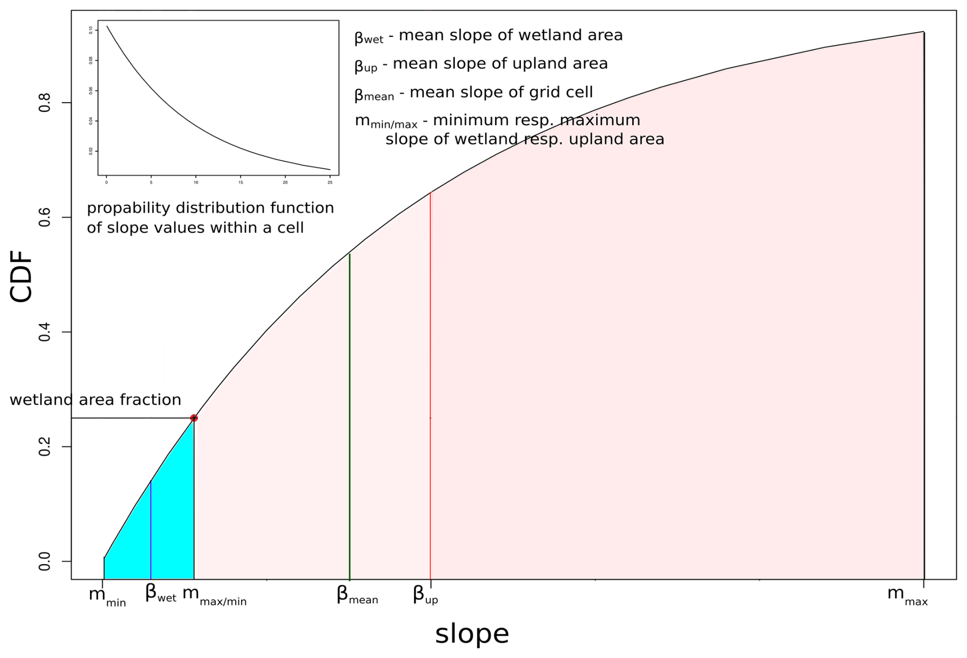
Figure 1 Determination of the slope values of wetland and upland stands depending on the fraction of the wetland area within a grid cell.

2.3 Methane cycle

CH₄ dynamics within the terrestrial biosphere arise from both natural biogeochemical cycles and anthropogenic influences. Natural CH₄ emissions are predominantly driven by anaerobic microbial methanogenesis in O₂-deprived environments such as wetlands, peatlands, and rice paddies, where the decomposition of organic matter under anoxic conditions facilitates CH₄ production. Anthropogenic processes – such as those associated with intensive livestock farming, rice cultivation, fossil fuel extraction, and land-use modifications – contribute additional CH₄ through altered substrate availability and ecosystem disruption. Within LPJmL 6.0, soil CH₄ dynamics are resolved at sub-daily time steps that simulate the CH₄ pool by accounting for concurrent production and oxidation (see Fig. 2). The CH₄ flux to the atmosphere is computed as the sum of ebullition, molecular diffusion, and plant-mediated transport. The magnitude of each pathway responds to soil moisture (saturation and air-filled porosity), substrate availability (labile carbon), and the soil redox state (oxygen availability), which together regulate both production and oxidation rates.

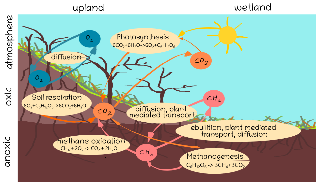
Figure 2 Newly added or modified soil processes in the LPJmL6 model. CO₂ diffusion is assumed to be instantaneous as in earlier versions of LPJmL (Schaphoff et al., 2018) and there is no interaction of CO₂ with the soil during the diffusion process, whereas the diffusion processes of oxygen and CH₄ are explicitly modeled because the time and position in the soil column is important for the CH₄ dynamics.

2.3.1 Balance of Methane and Oxygen Concentrations in Soils

The evolution of the CH₄ concentration in the soil is characterized by the diffusive transport of CH₄ through the soil column (first part of the equation) and the production of CH₄ (methanogenesis (R_prod)) and losses through CH₄ oxidation above the water saturated layer if enough oxygen is available (R_oxic), the de-gassing through forming of bubbles in water filled pores (ebullition (Q_ebull)), and the plant mediated transport ($Q_{\mathrm{plant},{\mathrm{CH}}_{\mathrm{4}}}$) by vascular plants through their aerenchyma:

$$\begin{array}{}\text{(26)}& \begin{array}{rl}{\displaystyle }{\mathit{ϵ}}_{{\mathrm{CH}}_{\mathrm{4}}}& {\displaystyle \frac{\partial C_{{\mathrm{CH}}_{\mathrm{4}}}(z,t)}{\partial t}}={\displaystyle \frac{\partial }{\partial z}}\left[D_{{\mathrm{CH}}_{\mathrm{4}}}\left(z\right){\displaystyle \frac{\partial C_{{\mathrm{CH}}_{\mathrm{4}}}(z,t)}{\partial z}}\right]\\ {\displaystyle }& {\displaystyle }-Q_{\mathrm{ebull}}^{\mathrm{out}}(z,t)+Q_{\mathrm{ebull}}^{\mathrm{in}}(z,t)-Q_{\mathrm{plant},{\mathrm{CH}}_{\mathrm{4}}}(z,t)\\ {\displaystyle }& {\displaystyle }+R_{\mathrm{prod}}(z,t)-R_{\mathrm{oxic}}(z,t).\end{array}\end{array}$$

The O₂ concentration is calculated analogously to the CH₄ concentration equation including the O₂ consuming processes of oxic decomposition of soil organic matter ($R_{{\mathrm{CO}}_{\mathrm{2}}}$),the plant mediated transport ($Q_{\mathrm{plant},{\mathrm{O}}_{\mathrm{2}}}$), nitrification of NH${}_{\mathrm{4}}^{+}$ to NO${}_{\mathrm{3}}^{-}$ ($R_{{\text{NO}}_{\mathrm{3}}^{-}}$), and aerobic root respiration (R_root):

$$\begin{array}{}\text{(27)}& \begin{array}{rl}{\displaystyle }{\mathit{ϵ}}_{{\mathrm{O}}_{\mathrm{2}}}\left(z\right)& {\displaystyle \frac{\partial C_{{\mathrm{O}}_{\mathrm{2}}}(z,t)}{\partial t}}={\displaystyle \frac{\partial }{\partial z}}\left[D_{{\mathrm{O}}_{\mathrm{2}}}\left(z\right){\displaystyle \frac{\partial C_{{\mathrm{O}}_{\mathrm{2}}}(z,t)}{\partial z}}\right]\\ {\displaystyle }& {\displaystyle }-Q_{\mathrm{plant},{\mathrm{O}}_{\mathrm{2}}}(z,t)\\ {\displaystyle }& {\displaystyle }-{\displaystyle \frac{W_{{\mathrm{O}}_{\mathrm{2}}}}{W_{\mathrm{C}}}}{R}_{{\mathrm{CO}}_{\mathrm{2}}}(z,t)-\mathrm{2}{\displaystyle \frac{W_{{\mathrm{O}}_{\mathrm{2}}}}{W_{{\mathrm{CH}}_{\mathrm{4}}}}}{R}_{\text{oxic}}(z,t)\\ {\displaystyle }& {\displaystyle }-\mathrm{2}{\displaystyle \frac{W_{{\mathrm{O}}_{\mathrm{2}}}}{W_{\mathrm{N}}}}{R}_{{\mathrm{NO}}_{\mathrm{3}}^{-}}(z,t)-{\displaystyle \frac{W_{{\mathrm{O}}_{\mathrm{2}}}}{W_{\mathrm{C}}}}{R}_{\text{root}}(z,t).\end{array}\end{array}$$

where ${\mathit{ϵ}}_{{\mathrm{O}}_{\mathrm{2}}}$ resp. ${\mathit{ϵ}}_{{\text{CH}}_{\mathrm{4}}}$ are the O₂ and CH₄ porosities, that convert concentration per soil volume to the gas concentration per air volume and are calculated as

$$\begin{array}{}\text{(28)}& {\mathit{ϵ}}_{{\text{O}}_{\mathrm{2}}}=v+\mathit{\varphi }\cdot {\mathit{\theta }}_{\mathrm{sat}}\cdot B_{{\text{O}}_{\mathrm{2}}},{\mathit{ϵ}}_{{\text{CH}}_{\mathrm{4}}}=v+\mathit{\varphi }\cdot {\mathit{\theta }}_{\mathrm{sat}}\cdot B_{{\text{CH}}_{\mathrm{4}}},\end{array}$$

where ϕ is the volumetric soil water content expressed per unit pore volume (mm³ of water per mm⁻³ of soil porous volume; here θ_sat is used as an equivalent measure of the pore‐volume fraction), and v is the soil air content (m³ air per m³ soil). W_C, $W_{{\text{O}}_{\mathrm{2}}}$, and $W_{{\text{CH}}_{\mathrm{4}}}$ are the molar masses of Carbon (12 g mol⁻¹), O₂ (32 g mol⁻¹), and CH₄ (16 g mol⁻¹), respectively. The Bunsen coefficients of O₂ ($B_{{\mathrm{O}}_{\mathrm{2}}}$) and CH₄ ($B_{{\mathrm{CH}}_{\mathrm{4}}}$) describe the solubility of these gases in water as a function of temperature. Due to the decreasing capacity of water to dissolve gases with rising temperature, this dependence is commonly expressed using exponential decay functions. Following Yamamoto et al. (1976) and Wiesenburg and Guinasso (1979), we apply the following empirical relationships:

$$\begin{array}{}\text{(29)}& \begin{array}{rl}{B}_{{\mathrm{O}}_{\mathrm{2}}}& =\mathrm{0.0647}\cdot e^{-\mathrm{0.0257}\cdot T_{\mathrm{soil}}},\\ & B_{{\mathrm{CH}}_{\mathrm{4}}}=\mathrm{0.0523}\cdot e^{-\mathrm{0.0236}\cdot T_{\mathrm{soil}}}.\end{array}\end{array}$$

The net CH₄ flux to the atmosphere, F_atm, represents the total upward CH₄ transfer from the soil to the atmosphere. It is considered positive when the soil acts as a net CH₄ source and negative when it acts as a net sink. This flux is composed of three contributing terms

$$\begin{array}{}\text{(30)}& \begin{array}{rl}{F}_{\text{atm}}\left(t\right)& ={\left(-D_{{\mathrm{CH}}_{\mathrm{4}}}\left(z\right){\displaystyle \frac{\partial C_{{\mathrm{CH}}_{\mathrm{4}}}(z,t)}{\partial z}}\right)}_{z=\mathrm{0}}+Q_{\mathrm{ebull}}^{\mathrm{out}}(\mathrm{0},t)\\ & +F_{\mathrm{plant}}\left(t\right),\end{array}\end{array}$$

where the diffusive flux at the soil-atmosphere interface, $-D_{{\mathrm{CH}}_{\mathrm{4}}}\left(z\right)\frac{\partial C_{{\mathrm{CH}}_{\mathrm{4}}}(z,t)}{\partial z}$, and the ebullition flux, $Q_{\text{ebull}}^{\mathrm{out}}(z=\mathrm{0},t)$, escape directly to the atmosphere. Note that ebullition contributes directly to the atmospheric flux only from the surface layer (z=0), as ebullition from deeper layers is transferred to the layer above instead of escaping directly (see Sect. 2.3.5). The third term, F_plant(t), represents the flux of CH₄ transported through plant tissues (see Sect. 2.3.6), particularly aerenchyma structures, which provide a low-resistance conduit for CH₄ transfer from anaerobic soil layers directly to the atmosphere, bypassing diffusion and ebullition pathways.

2.3.2 Soil organic matter decomposition into CO₂ and CH₄

Oxic decomposition of organic carbon follows the principles described by Schaphoff et al. (2018). The anoxic decomposition model is adapted from Khvorostyanov et al. (2008). Aerobic conditions promote the generation of CO₂ in all soil carbon pools and anaerobic conditions lead to CH₄ production. The soil carbon pools consist of an intermediate and a slow pool with turnover rates for the oxic decomposition of 0.03 and 0.001 respectively at 10 °C and a fast so-called active pool with a turnover rate of 0.3 (Schaphoff et al., 2018). For realistic decomposition dynamics, Schaphoff et al. (2013) introduced a vertical soil distribution (Jobbagy and Jackson, 2000) which improved the simulation of the carbon, which can be released by permafrost thawing (see also Schaphoff et al., 2013). Decomposition follows first order kinetics:

$$\begin{array}{}\text{(31)}& {\displaystyle \frac{\partial C(z,t)}{\partial t}}=R_{{\mathrm{CO}}_{\mathrm{2}}}(z,t)-R_{\mathrm{prod}}(z,t)\cdot {\displaystyle \frac{W_{\mathrm{C}}}{W_{{\mathrm{CH}}_{\mathrm{4}}}}},\end{array}$$

where oxic ($R_{{\mathrm{CO}}_{\mathrm{2}}}$) and anoxic decomposition (R_prod) is reciprocally exclusive.

Soil respiration – oxic decomposition

Oxic decomposition is computed as

$$\begin{array}{}\text{(32)}& R_{{\text{CO}}_{\mathrm{2}}}(z,t)=\text{min}\left[k_{\mathrm{1}}(z,t)\cdot C(z,t),{\displaystyle \frac{\partial C_{\text{max}}(z,t)}{\partial t}}\right]\end{array}$$

where C is the carbon pool size at time t and soil depth z, k₁ is the daily oxic decomposition rate, and ∂C_max is the mass of carbon corresponding to O₂ which is available for oxic decomposition:

$$\begin{array}{}\text{(33)}& {\displaystyle \frac{\partial C_{\text{max}}(z,t)}{\partial t}}={\text{O}}_{\mathrm{2}}(z,t)\cdot {\displaystyle \frac{W_{\text{C}}}{W_{{\text{O}}_{\mathrm{2}}}}}\end{array}$$

O₂(z) is the mass of molecular soil O₂ at depth z. The oxic decomposition rate is expressed as:

$$\begin{array}{}\text{(34)}& k_{\mathrm{1}}(z,t)=k\cdot g\left(T_{\text{soil}}\right(z,t\left)\right)\cdot f\left(\mathit{\varphi }\left(z\right)\right).\end{array}$$

k₁ incorporates the rate constant (k) that represents the reciprocal of the mean residence time τ for the litter components, as described by Schaphoff et al. (2018) for the litter components. Additionally, k₁ is influenced by the temperature dependency function g(T_soil(z,t)), and the soil moisture function f(ϕ_z) as outlined in Schaphoff et al. (2018) related to the non–frozen water. The temperature dependence function is based on an Arrhenius relationship as described in Schaphoff et al. (2018)

$$\begin{array}{}\text{(35)}& \begin{array}{rl}& g\left(T_{\text{soil}}(z,t)\right)=\\ & \exp [\mathrm{308.56}\cdot ({\displaystyle \frac{\mathrm{1}}{\mathrm{56.02}}}-{\displaystyle \frac{\mathrm{1}}{T_{\mathrm{soil}}(z,t)+\mathrm{46.02}}}\left)\right],\end{array}\end{array}$$

where T_soil is the soil temperature in degree Celsius. The soil moisture function has its maximum around field capacity of the soil and is given by

$$\begin{array}{rl}f\left(\mathit{\varphi }\right(z\left)\right)& =\mathrm{0.0402}-\mathrm{5.005}\cdot \mathit{\varphi }(z{)}^{\mathrm{3}}\\ & +\mathrm{4.269}\cdot \mathit{\varphi }(z{)}^{\mathrm{2}}+\mathrm{0.719}\cdot \mathit{\varphi }(z).\end{array}$$

Methanogenesis – anoxic decomposition

The anoxic decomposition (R_prod) is calculated as follows:

$$\begin{array}{}\text{(36)}& R_{\text{prod}}(z,t)=k_{\mathrm{2}}(z,t)\cdot C(z,t).\end{array}$$

The methanogenesis rate (k₂) is expressed as

$$\begin{array}{}\text{(37)}& k_{\mathrm{2}}(z,t)=k\cdot r_k\cdot \exp \left({\displaystyle \frac{-C_{{\text{O}}_{\mathrm{2}}}(z,t)}{{\mathrm{O}}_{\mathrm{2}}^{*}}}\right)\cdot g\left(T_{\text{soil}}\right(z,t\left)\right).\end{array}$$

$C_{{\text{O}}_{\mathrm{2}}}(z,t)$ is the O₂ concentration at depth z, while O${}_{\mathrm{2}}^{*}$ represents a threshold O₂ concentration of 10 g m⁻³. As demonstrated by Duval and Goodwin (2000) methanogenesis is significantly suppressed by higher O₂ concentrations. r_k is an empirical parameter reflecting the reduced methanogenesis rate under anoxic conditions, which is considerably slower than oxic decomposition and is set to 0.1 for the fast soil carbon pool and 0.5 for the fast decomposing litter pool. Components of the carbon pool, such as lignin, degrade much more slowly in anoxic environments due to their recalcitrant structure and resistance to microbial breakdown, further limiting methanogenesis. The decomposition rate under anoxic conditions is 4–10 times lower than under oxic conditions, with reported rates ranging from 0.02 to 1.44 mg CH₄ g⁻¹ over 500 d (Lee et al., 2012). This corresponds to a decomposition rate between $\mathrm{1.46}\times {\mathrm{10}}^{-\mathrm{5}}$ and 0.00105. Methanogenesis rate k₂ has the same temperature dependence g(T_soil(z,t)) and rate constant (k) as the oxic decomposition.

2.3.3 Methane oxidation (R_oxic)

The representation of the CH₄ oxidation (R_oxic) follows the approach by Walter and Heimann (2000). R_oxic occurs above the saturated soil layer, where enough O₂ is available.

$$\begin{array}{}\text{(38)}& \begin{array}{rl}{R}_{\text{oxic}}(z,t)& =min[{\displaystyle \frac{V_{max}\cdot W_{{\text{CH}}_{\mathrm{4}}}\cdot C_{{\text{CH}}_{\mathrm{4}}}\left(z,t\right)}{K_{\text{m}}\cdot W_{{\text{CH}}_{\mathrm{4}}}+C_{{\text{CH}}_{\mathrm{4}}}\left(z,t\right)}}\\ & \cdot g\left(T_{\text{soil}}\left(z,t\right)\right),C_{{\text{O}}_{\mathrm{2}}}\left(z,t\right)\cdot {\displaystyle \frac{W_{{\text{CH}}_{\mathrm{4}}}}{\mathrm{2}{W}_{{\text{O}}_{\mathrm{2}}}}}\cdot {\text{O}}_{\mathrm{2},\text{frac}}],\end{array}\end{array}$$

where K_m and V_max are the Michaelis-Menten coefficients. These are defined in the model for K_m=5 µM and $V_{max}=\mathrm{20}$ µM h⁻¹ (Walter and Heimann, 2000). $C_{{\text{CH}}_{\mathrm{4}}}$ is the CH₄ concentration at time t and depth z in g m⁻³. g(T_soil) is the temperature response function given in Eq. (35). V_max and K_m need to be multiplied by the molecular mass of CH₄. O₂ consumption is limited by O${}_{\mathrm{2},\text{frac}}=\mathrm{0.95}$, accounting for O₂ use for oxidation of reduced compounds, where 5 % is assumed (Conrad, 1996; Xu et al., 2010; Saunois et al., 2020). O₂ consumption from aerobic microbial respiration, plant root respiration. nitrification and CH₄ oxidation is taken into account by reducing the O₂ content of the respective layer.

For the temperature dependency of CH₄ oxidation a Q₁₀ relationship is used

$$\begin{array}{}\text{(39)}& g\left(T_{\text{soil}}(z,t)\right)=Q_{\mathrm{10}}^{\frac{T_{\text{soil}}(z,t)-T_{\text{soil,mean}}\left(z\right)}{\mathrm{10}}}\end{array}$$

where T_soil,mean is the annual mean soil temperature and the Q₁₀ is set to 1.8.

2.3.4 Diffusion of Methane from soil (F_diff)

CH₄ diffusion, which describes the movement of gas from higher to lower concentrations between layers and the air, is governed by Fick’s law:

$$\begin{array}{}\text{(40)}& F_{\text{diff}}\left(z,t\right)=D_{{\text{CH}}_{\mathrm{4}}}\left(z\right)\cdot {\displaystyle \frac{\partial C_{{\text{CH}}_{\mathrm{4}}}}{\partial x}}\left(z,t\right),\end{array}$$

where $D_{{\text{CH}}_{\mathrm{4}}}\left(z\right)$ is the diffusivity at depth z and $C_{{\text{CH}}_{\mathrm{4}}}\left(z,t\right)$ is the CH₄ concentration at time t and depth z. $D_{{\mathrm{CH}}_{\mathrm{4}}}$ is calculated depending on soil water conditions:

$$\begin{array}{}\text{(41)}& D_{{\mathrm{CH}}_{\mathrm{4}}}=(D_{{\text{air}}_{{\mathrm{CH}}_{\mathrm{4}}}}\cdot v+D_{{\text{water}}_{{\mathrm{CH}}_{\mathrm{4}}}}\cdot w\cdot {\mathit{\theta }}_{\text{sat}}\cdot B_{{\text{CH}}_{\mathrm{4}}})\cdot \mathit{\eta }\end{array}$$

where $D_{{\text{air}}_{{\mathrm{CH}}_{\mathrm{4}}}}$ is the diffusivity of air ($\mathrm{1.82}\times {\mathrm{10}}^{-\mathrm{5}}$ m² s⁻¹, Massman, 1998) and $D_{{\text{water}}_{{\mathrm{CH}}_{\mathrm{4}}}}$ the diffusivity of water ($\mathrm{1.6}\times {\mathrm{10}}^{-\mathrm{9}}$ m² s⁻¹, Khvorostyanov et al., 2008). $B_{{\text{CH}}_{\mathrm{4}}}$ is the Bunsen coefficient for CH₄ (see Eq. 29) and $\mathit{\eta }=\mathrm{2}/\mathrm{3}$ denotes the soil tortuosity. O₂ diffusion is calculated analogous to Eqs. (40) and (41). Initial conditions of all soil layers are:

$$\begin{array}{ll}{\displaystyle }{\text{C}}_{{\text{CH}}_{\mathrm{4}}}& {\displaystyle }=\mathrm{1.207}{\text{ g\hspace{0.17em}m}}^{-\mathrm{3}},\\ {\displaystyle }{\text{C}}_{{\text{O}}_{\mathrm{2}}}& {\displaystyle }=\mathrm{266}{\text{ g\hspace{0.17em}m}}^{-\mathrm{3}}\end{array}$$

The lower boundary for both CH₄ and O₂ conditions are:

$$\begin{array}{}\text{(42)}& {\displaystyle \frac{\partial C_{{\mathrm{CH}}_{\mathrm{4}}}(z=\mathrm{soildepth})}{\partial z}}={\displaystyle \frac{\partial {\mathrm{O}}_{\mathrm{2}}(z=\mathrm{soildepth})}{\partial z}}=\mathrm{0}\end{array}$$

and the upper boundary conditions are:

$$\begin{array}{}\text{(43)}& C(z=\mathrm{0})={\displaystyle \frac{p_{\mathrm{s}}}{R\cdot T_{\text{air}}}}\cdot {\text{AC}}_{\text{gas}}\cdot W,\end{array}$$

where p_s is the atmospheric surface pressure (101 000 Pa), T_air is the air temperature (in K), AC_gas is the atmospheric content (0.209 for O₂, transient over time for CH₄), W is the molar mass of O₂ and CH₄, respectively and R is the universal gas constant (8.314 J mol⁻¹ K⁻¹).

2.3.5 Methane ebullition (Q_ebull)

CH₄ ebullition is the process by which CH₄ gas produced in anaerobic soil environments escapes into the atmosphere through gas bubbles. This occurs when the concentration of dissolved CH₄ in soil porewater exceeds its solubility threshold, causing bubble nucleation and release. The process is modulated by factors such as CH₄ concentration, soil moisture, and vegetation cover, which influence both the formation and migration of gas bubbles. The change in CH₄ concentration in a soil layer over time due to ebullition is governed by a balance between CH₄ loss via ebullition and CH₄ flux received from the layer below.

Ebullition is active only when the local CH₄ concentration exceeds a critical threshold required for bubble formation (Walter and Heimann, 2000), and the outgoing ebullition flux is then calculated as

$$\begin{array}{}\text{(44)}& Q_{\text{ebull}}^{\text{out}}(z,t)=k_{\mathrm{e}}\cdot max\left(\right(C_{{\text{CH}}_{\mathrm{4}}}(z,t)-C_{\text{thresh}}),\mathrm{0}),\end{array}$$

where k_e is the ebullition efficiency constant controlling the rate of CH₄ release, which typically ranges between 0.1 to 1 d⁻¹, and C_thresh is the threshold CH₄ concentration for bubble formation. In this study we set k_e=1. The functional form of the threshold concentration is given by

$$\begin{array}{}\text{(45)}& C_{\text{thresh}}=C_{\text{min}}\cdot \left(\mathrm{1}+\mathrm{1}-\sum _{\text{pft}=\mathrm{1}}^{n_{\text{PFT}}}({\mathit{\alpha }}_{\text{pft}}^e\cdot {\text{FPC}}_{\text{pft}})\right),\end{array}$$

Experimental studies have shown that the presence of vegetation can substantially suppress CH₄ ebullition due to competition with plant-mediated transport and structural alterations to sediment or soil (Deshmukh et al., 2020). Therefore, to represent the vegetation-dependent reduction in ebullition flux, we introduce plant functional type (PFT)-specific suppression (α^e) factors in the model (see Tables S3 and S4 for parameter values). These account for the observed differences in ebullition across vegetated and non-vegetated systems, as supported by field measurements. FPC is the fractional plant cover of the PFT, which influences bubble formation by altering gas exchange dynamics. C_min is the minimum CH₄ concentration required for bubble formation under standard conditions and has been observed to range between 500 and $\mathrm{1000}\times {\mathrm{10}}^{-\mathrm{6}}$ M (Khvorostyanov et al., 2008) which corresponds to 0.008 to 0.016 g m⁻³. We use 0.012 g m⁻³ in LPJmL6. Eq. (44) ensures that ebullition only occurs when the gas pressure exceeds the critical pressure threshold.

The outgoing ebullition flux is transferred upwards and is added to the incoming ebullition flux $Q_{\mathrm{ebull}}^{\mathrm{in}}(z,t)$ in a layer above in case of z<0, or to the atmosphere in case of z=0. At the shallowest soil depth, there is no overlying material to impede the upward migration of gas bubbles. Therefore, the ebullition flux originating from this depth contributes directly to the CH₄ flux emitted to the atmosphere.

At deeper soil depths, the fate of CH₄ released via ebullition depends on the moisture content of the overlying soil column. If the overlying layer is not saturated (θ<0.9), the bubbles are trapped and remain in the overlying layer, preventing direct transfer. However, if the overlying layer is water-saturated (soil moisture >0.9), bubbles migrate further upward and are transferred to the next layer above.

This recursive upward propagation continues through the saturated soil profile until an unsaturated soil layer is found or the surface is reached. This mechanism determines whether CH₄ from deeper soil zones contributes to atmospheric emissions or remains retained within the subsurface environment.

2.3.6 Plant-Mediated Transport (Q_plant)

Certain vascular plants possess aerenchyma, a specialized tissue forming interconnected air-filled channels within their stems, leaves, and roots. This tissue facilitates the movement of O₂ and CH₄ between the plant and its environment, playing a crucial role in gas exchange, particularly in waterlogged or anaerobic soils. O₂ is transported from the atmosphere through the stems and leaves into the roots, supporting root respiration. Conversely, CH₄ produced in anaerobic soils can diffuse into the aerenchyma through the roots and be transported upward through the plant, being released into the atmosphere, bypassing the oxidizing zones in the soil. We hypothesize that this gas exchange via aerenchyma is more prominent in grasses compared to trees, as aerenchyma is predominantly observed in herbaceous plants and is largely absent in woody species (Takahashi et al., 2014; Colmer, 2003). To quantify these processes, we adopt the approach outlined by Wania et al. (2010) which shows that gas diffusion through aerenchyma (F_plant) depends on both the cross-sectional area of plant tillers available for gas transport (A_tiller, in m²) and the volumetric soil liquid water content (θ_liq, in m³):

$$\begin{array}{}\text{(46)}& F_{\text{plant}}\left(t\right)=\stackrel{\text{soilsurface}}{\underset{\text{rootingdepth}}{\int }}{Q}_{\text{plant}}\left(z,t\right)\cdot \text{d}z,\end{array}$$

where

$$\begin{array}{}\text{(47)}& \begin{array}{rl}{Q}_{\text{plant}}(z,t)& =\left(C_{\text{gas}}(z,t)-C_{\text{gas}{}_{\text{air}}}\right)\\ & \cdot \exp \left({\displaystyle \frac{-k_{\text{gas}}\cdot A_{\mathrm{tiller}}}{{\mathit{\theta }}_{\text{liq}}(z,t)}}\right).\end{array}\end{array}$$

This equation is applied to both O₂ and CH₄ in the model, reflecting the bidirectional transport of these gases. A_tiller is defined as:

$$\begin{array}{}\text{(48)}& A_{\text{tiller}}=max\left(\mathrm{0.001},\mathit{\pi }\cdot r_{\text{tiller}}^{\mathrm{2}}\cdot N_{\text{tiller}}\cdot {\mathit{\varphi }}_{\text{tiller}}\right),\end{array}$$

where r_tiller is the radius of an individual plant tiller defined to be r_tiller=0.0345 m (Nascimento et al., 2021). The variable ϕ_tiller is the porosity of the tiller structure, expressed as a dimensionless fraction (ϕ_tiller=0.7). The use of the max function ensures that A_tiller maintains a minimum value of 0.001 m², preventing numerical instability when the calculated tiller area becomes very small. N_tiller represents the tiller fraction, which depends on plant biomass and root distribution within the soil layer:

$$\begin{array}{}\text{(49)}& N_{\text{tiller}}={\text{C}}_{\mathrm{leaf}}\cdot (\mathit{\gamma }/W_{\mathrm{tiller}})\cdot F_{\mathrm{root}\left(l\right)},\end{array}$$

where C_leaf is the leaf carbon per square meter for PFTs that are able to form aerenchyma and γ is the phenology status of the PFT. W_tiller=0.22 g (Wania et al., 2010) is the weight of the tillers and F_root(l) is the fraction of the root in the respective layer.

The gas exchange coefficient, (k_gas in m d⁻¹), represents the piston velocity between the water and the atmosphere. Following Wania et al. (2010), (k_gas) is obtained by scaling a reference transfer velocity for a Schmidt number (Sc) of 600, (k₆₀₀=2.07 m d⁻¹) with the actual Schmidt number of the respective gas:

$$\begin{array}{}\text{(50)}& k_{\text{gas}}=k_{\mathrm{600}}\cdot {\left({\displaystyle \frac{S{c}_{\mathrm{gas}}}{\mathrm{600}}}\right)}^{n_p},\end{array}$$

where n_p is the Schmidt-number exponent, here set to −0.5. Sc can be calculated specifically for O₂ and CH₄:

$$\begin{array}{}\text{(51)}& S{c}_{{\mathrm{CH}}_{\mathrm{4}}}=\mathrm{1898}-\mathrm{110.1}\cdot T_{\mathrm{air}}+\mathrm{2.834}\cdot T_{\mathrm{air}}^{\mathrm{2}}-\mathrm{0.02791}\cdot T_{\mathrm{air}}^{\mathrm{3}}\end{array}$$

and

$$\begin{array}{}\text{(52)}& \begin{array}{rl}S{c}_{\mathrm{O}{}_{\mathrm{2}}}& =\mathrm{1800.6}-\mathrm{120.1}\cdot T_{\mathrm{air}}+\mathrm{3.7818}\cdot T_{\mathrm{air}}^{\mathrm{2}}\\ & -\mathrm{0.047608}\cdot T_{\mathrm{air}}^{\mathrm{3}}\end{array}\end{array}$$

In summary, CH₄ and O₂ fluxes are based on concentration gradients, gas transfer velocities, and tiller geometry, while accounting for soil moisture, porosity, and air content. These fluxes reflect the dynamic movement of gases between the soil and atmosphere, influenced by soil properties, plant structure, and environmental conditions.

2.3.7 Oxygen consumption by nitrification and root respiration

Dissolved oxygen in each soil layer is consumed by nitrification of ammonium and aerobic root respiration. Nitrification is represented by the overall reaction

$${\mathrm{NH}}_{\mathrm{4}}^{+}+\mathrm{2}{\mathrm{O}}_{\mathrm{2}}\to {\mathrm{NO}}_{\mathrm{3}}^{-}+\mathrm{2}{\mathrm{H}}^{+}+{\mathrm{H}}_{\mathrm{2}}\mathrm{O},$$

i.e. one mole of N nitrified requires two moles of O₂. For the nitrification rate $R_{{\mathrm{NO}}_{\mathrm{3}}^{-}}(z,t)$ (g N m⁻³ s⁻¹), the associated O₂ consumption is

$$\begin{array}{}\text{(53)}& S_{{\mathrm{O}}_{\mathrm{2}}}^{\text{nitr}}(z,t)=\mathrm{2}{\displaystyle \frac{W_{{\mathrm{O}}_{\mathrm{2}}}}{W_{\mathrm{N}}}}{R}_{{\mathrm{NO}}_{\mathrm{3}}^{-}}(z,t),\end{array}$$

where W_N is the molar mass of N (14 g mol⁻¹). In the numerical implementation $R_{{\mathrm{NO}}_{\mathrm{3}}}(z,t)$ corresponds to the depth-dependent analogue of the nitrification flux $F_{{\mathrm{NO}}_{\mathrm{3}}^{-}}$ limited by O₂, NH${}_{\mathrm{4}}^{+}$ availability, soil moisture, temperature and pH (see von Bloh et al., 2018).

Aerobic root respiration represents the metabolic consumption of O₂ by living roots to sustain maintenance and growth. The model provides a depth-dependent root respiration rate R_root(z,t) (g C m⁻³ s⁻¹), which is distributed over the soil profile according to the vertical root density. Because the O₂ balance is formulated in units of O₂ mass, this carbon–based respiration flux is converted into an equivalent O₂ sink $S_{{\mathrm{O}}_{\mathrm{2}}}^{\text{root}}$ using a constant mass-conversion factor, yielding

$$\begin{array}{}\text{(54)}& S_{{\mathrm{O}}_{\mathrm{2}}}^{\text{root}}(z,t)={\displaystyle \frac{W_{{\mathrm{O}}_{\mathrm{2}}}}{W_{\mathrm{C}}}}{R}_{\text{root}}(z,t).\end{array}$$

2.3.8 Numerical scheme

Numerical solutions to the CH₄ and O₂ diffusion equations are obtained using the finite difference method for the heat diffusion problem described by Alexiades and Solomon (1993, Sect. 4.1). For time stepping the forward Euler, Crank-Nicolson and backward Euler methods were tested. The backward Euler scheme was the only method that provided sufficient stability and was thus chosen for the solution of the diffusion problems. All other elements of the methane and oxygen balance, including the reaction terms, are solved using the forward Euler method.

Experiments with the time step showed that the default daily time step of LPJmL is not sufficient to obtain accurate and stable numerical solutions for the coupled methane and oxygen balance. A baseline sub-daily time step of 4 h was therefore adopted. Additionally, an adaptive sub-stepping scheme was implemented that rejects this baseline time step and reduces it to six 40 min increments whenever the baseline time step causes a relative change of CH₄ or O₂ concentration larger than 20 % in any soil layer.

The numerical errors resulting from the temporal discretization were estimated by performing a global run of LPJmL6 using a smaller baseline time step of 80 min while leaving the adaptive sub-stepping scheme untouched. The global sum and temporal mean of CH₄ and O₂ concentrations in soils changed by less than 1 % compared to the default 4 h baseline time step. Global methane emissions decreased by 5.2 % when switching to the increased temporal resolution.

2.4 Inundation feedback on vegetation

Inundation harms trees, grasses and crops that are not tolerant of water-saturated soils. These damages can cause (potentially lethal) productivity losses. The most important factor determining plant survival is the duration of inundation (Parolin and Wittmann, 2010). To account for the effect of inundation on vegetation we have introduced a feedback of inundation on gross primary production (GPP) and added three new PFTs which are tolerant to inundation: a tropical broadleaved evergreen flood-tolerant tree, a C3 graminoid herbaceous plant and sphagnum moss. The last two were already implemented in the LPJWhy model by Wania et al. (2009). The tropical tree is parameterized similarly to the default tropical broadleaved evergreen tree in previous LPJmL versions but with a parameterization tolerant of inundations.

Inundation areas are often not flooded constantly. To account for inundation stress we have introduced two new parameters as suggested by Wania et al. (2009). The inundation stress height (ist_m) defines at which water table depth a PFT experiences inundation stress and the inundation duration (idt_d) defines how long a PFT can endure inundation. The inundation-tolerant PFTs have a higher inundation stress height and endure longer inundation periods (Table S3). The stress factor (S_inun) is applied to GPP whenever the water table exceeds ist_m ($\mathrm{GPP}=\mathrm{GPP}\cdot (\mathrm{1}-S_{\text{inun}})$):

$$\begin{array}{}\text{(55)}& \begin{array}{rl}& S_{\text{inun}}=\\ & min\left(\mathrm{1},max\left(\mathrm{0},\left[{\displaystyle \frac{\mathrm{1}}{\mathrm{1}+\exp \left(-k\cdot (N_{\text{inun}}-{\mathrm{idt}}_d)\right)}}-\mathrm{0.5}\right]\times \mathrm{2}\right)\right),\end{array}\end{array}$$

where N_inun counts the number of days with inundation stress. Table S3 gives the parameter values of idt_d for the different PFTs, representing their tolerable inundation duration. Values from Wania et al. (2009) were adjusted, i.a. because PFTs TrBrEv and PoHe are not present in the implementation of Wania et al. (2009). The parameters for crop functional types (CFTs) in Table S4 take into account that the different CFTs suffer differently from inundation (Kaur et al., 2020). The parameter k (0.2 in d⁻¹) controls how rapidly stress increases once the inundation duration exceeds the threshold, with larger values producing a steeper rise. When the inundation threshold (ist_m) is no longer exceeded, the duration counter decreases in accelerated daily steps (five per day), representing a faster recovery of the plants relative to the length of the preceding inundation period.

Additionally, inundation stress increases tree mortality, contributing an additional mortality component (mort_inun) that increases the overall tree mortality rate. This contribution is capped at a maximum increase (inun_max) of 10 % relative to the potential mortality rate (mort_max):

$$\begin{array}{}\text{(56)}& {\text{mort}}_{\text{inun}}={\text{mort}}_{\text{max}}\cdot (\mathrm{1}-{\text{inun}}_{\text{max}}^{S_{\text{inun}}}),\end{array}$$

where mort_max represents the PFT-specific baseline mortality rate as described in Schaphoff et al. (2018).

2.5 Land-use change and rice cultivation

To account for the actual land cover, the model had to be extended for land-use change on wetlands. Previous versions of LPJmL distinguish a rainfed and an irrigated stand on which rainfed and irrigated crop cultivation as well as the off season is simulated, respectively. Here we assume that rice cultivation takes place on wetland areas if natural wetlands are present in the respective grid cell. Therefore, a new wetland setaside stand is introduced from which cropland is sourced for rice cultivation upon sowing/transplanting. If not enough upland (dry) natural land is available in the cell to satisfy land use demand, wetland area can also be converted to managed grasslands and, as a last resort, to cropland for crops other than rice. Soil water on rice fields is filled up above field capacity through irrigation to simulate permanent inundation. There is no explicit simulation of drainage systems for non-rice cultivation on wetland areas. A land use overview scheme is given in the Supplement Fig. S1.

3 Modelling protocol

To demonstrate the performance of LPJmL6 to model the newly implemented process dynamics, it was initialized with a spin-up period of 4000 years, using repeated climatic data from 1901 to 1930 to simulate pre-industrial conditions and achieve dynamic equilibrium in vegetation structure and composition as well as in carbon and nitrogen pools, representing a hypothetical stable pre-industrial state. To account for historical land-use dynamics, an additional 420 years of spin-up simulation were performed between the initial spin-up and the transient historical simulation, ensuring accurate representation of land-use history and its effects on biogeochemical pools and cycles. Following this, a transient simulation was conducted, covering the period 1901 to 2019.

4 Data used

4.1 Input data

LPJmL6 was here driven by GSWP3-W5E5 climate data (Lange et al., 2023) at a daily time step. This dataset combines W5E5 v2.0 (Cucchi et al., 2020; Lange et al., 2021) for the period 1979–2019 with GSWP3 v1.09 (Kim, 2017) for the period 1901–1978. GSWP3 data have been bias-adjusted towards W5E5 to reduce discontinuities at the 1978/1979 transition (Mengel et al., 2021). Annual atmospheric CO₂ concentrations are taken from the TRENDY project (Friedlingstein et al., 2023). Annual atmospheric CH₄ concentrations are taken from the NOAA Global Monitoring Laboratory (NOAA Global Monitoring Laboratory, 2025). Land-use data are generated with the LandInG toolbox (Ostberg et al., 2023). LandInG integrates and harmonises a number of gridded source datasets such as cropland and pasture extent from HYDE v3.2.1 (Klein Goldewijk et al., 2017a), multiple-cropping suitability from GAEZ v3 (IIASA/FAO, 2012), and crop-specific harvested areas for the year 2000 (Monfreda et al., 2008), with census data at national scale from FAOSTAT (FAO, 2020b), AQUASTAT (FAO, 2020a) and MIRCA2000 (Portmann et al., 2010a, b) to derive gridded time series of crop-specific growing patterns (with a distinction of rain-fed and irrigated areas) and pasture areas. As fallow land is currently not supported as a separate land-use category by LPJmL, fallow land from LandInG is assigned to the “others” crop category in LPJmL. LandInG also integrates crop-specific fertilizer application patterns for the year 2000 (Mueller et al., 2012; Mueller, 2012) with national-scale fertilizer application trends (Hurtt et al., 2020) to derive gridded time series of crop-specific nitrogen fertilizer application rates. Manure application rates are based on Zhang et al. (2017a, b). Crop-specific growing periods are based on the GGCMI phase 3 crop calendar (Jägermeyr et al., 2021). Grazing management is simulated on prescribed pasture areas (see above), with livestock densities based on Heinke (2025). Soil texture and soil acidity (pH) inputs are based on HWSD v1.21 (FAO/IIASA/ISRIC/ISSCAS/JRC, 2012), which has been aggregated from the source resolution by selecting parameters representative of the most prevalent soil type in each LPJmL grid cell (Ostberg et al., 2023). River network topology is based on STN-30 (Vörösmarty et al., 2000). Prescribed lake surface areas are based on GLWD (Lehner and Döll, 2004). Dam and reservoir characteristics are based on GRanD (Lehner et al., 2011; Biemans et al., 2011). Water use for households, industry and livestock in each grid cell is taken from Flörke et al. (2013) (prioritized over irrigation; accounting for 201 km³ in the year 2000). We use the ISLSCP II HYDRO1k elevation-derived products at 0.5° spatial resolution (Verdin et al., 2011), which provide, for each grid cell, statistics of the compound topographic index (CTI) including its mean, standard deviation and skewness; these moments are used to parameterise the gamma distribution of CTI in our wetland scheme (Sect. 2.1). The ISLSCP II product is derived from the original 1 km HYDRO1k database (U.S. Geological Survey, 2007b). The slope values are taken directly from the USGS fine-resolution 30 arcsec GTOPO30 slope product (U.S. Geological Survey, 2007a), from which we derive the mean, maximum and minimum slope of each 0.5° cell for the slope–dependent wetland parameterisation.

4.2 Validation data

A combination of geographically detailed data is used to evaluate the LPJmL6 model's ability to simulate wetland extent. Kaplan (2007) provides a global wetland map at 0.5° resolution, combining regional and global inventories, geomorphic and hydrological data, and satellite observations. It broadly defines wetlands, including permanently and seasonally inundated areas, and waterlogged soils. The Global Lakes and Wetlands Database (GLWD) by Lehner and Döll (2004) offers high-resolution (1 km) data on lakes, reservoirs, and wetlands, classifying water bodies by size, hydrology, and ecological features. While we use the GLWD lake area as an input to the model (Sect. 4.1) we use the GLWD wetland extent for validating the simulated global dynamics of wetland extent. Gumbricht et al. (2017) present the SWAMP dataset, a high-resolution (231 m) map of tropical and subtropical wetlands, integrating geomorphic classification, hydrological modeling, and satellite imagery. Zhang et al. (2021a) developed WAD2M, a dataset on monthly wetland extent for 2000–2018 at 25 km resolution (using the mean annual extent), focused on permanently vegetated wetlands by excluding permanent water bodies, coastal wetlands, and rice paddies.

Estimates of CH₄ emissions from rice cultivation were derived from a combination of empirical field data, synthesis studies, and global-scale inverse modeling frameworks, as follows. The resulting CH₄ emission values represent cumulative seasonal emissions (in gCH₄ m⁻²) from flooded rice systems, calculated by multiplying observed or reported mean daily CH₄ emission rates (gCH₄ m⁻² d⁻¹) with region-specific growing season lengths. This approach allows for spatially explicit interregional comparison of seasonal CH₄ release, facilitating benchmarking of biogeochemical models and identifying emission hotspots. A comprehensive synthesis by Wang et al. (2018) compiled over 600 site-years of CH₄ flux data collected from 1990 to 2014, encompassing diverse rice-growing environments and management regimes. Their dataset provided country-level mean emission rates and associated 95 % confidence intervals, reflecting spatial heterogeneity across sites. These values were further stratified by continent and climate zone to support global upscaling. Complementing this synthesis, Zhu and Li (2024) incorporated more recent CH₄ flux observations from East Asia, including multi-cropping systems and long-term experimental sites. Their dataset included some of the highest recorded emissions, particularly in southern China, and expanded the representativeness of regional variability. In South Asia, Gupta et al. (2021) reported empirical data on daily CH₄ fluxes from irrigated rice paddies in northern India under varying water and residue management practices, highlighting the mitigation potential of alternate wetting and drying regimes. Earlier field-based estimates provided by Wassmann et al. (2000) focused on major rice ecosystems in Southeast Asia, using controlled experiments and standardized chamber measurements under the IRRI-GTZ collaboration. Their regional emission ranges from the 1990s remain influential for emission factor development and baseline scenario assessment.

While these sources generally provide spatial uncertainty bounds, they do not fully capture interannual variability, which may be significant under shifting climate and agronomic conditions. To contextualize and constrain bottom-up estimates, we integrated global atmospheric inversion data from the CarbonTracker-CH₄ framework (NOAA Global Monitoring Laboratory, NOAA Global Monitoring Laboratory (2025); Bruhwiler et al. (2014)). This system assimilates atmospheric CH₄ concentrations from NOAA’s global flask and in situ measurement network (NOAA Global Monitoring Laboratory, 2025) to infer regional and global emission patterns. Wetland and rice cultivation emissions were treated as distinct sectors, enabling partial attribution of seasonal CH₄ enhancements to rice-growing regions in Asia. Additional global source data and attribution uncertainty ranges were taken from the Global Methane Budget reports by Saunois et al. (2020, 2025), which combine bottom-up inventories, top-down atmospheric inversions, and process-based models. To analyze how CH₄ emissions vary with latitude across different datasets, the LPJmL6 model is compared with the WetCHARTs v1.0 dataset provided by Bloom et al. (2017a). WetCHARTs (Wetland and Climate CH₄ Intercomparison of Models) offers a global dataset of wetland CH₄ emissions at a 0.5° resolution, along with associated uncertainties. This dataset integrates multiple emission models, remote sensing data, and atmospheric observations to provide a comprehensive and harmonized view of CH₄ emissions from wetlands.

Monthly river discharge observations were used to evaluate monthly simulated river discharge at the basin scale. The observational compilation comprises 285 gauging stations with reported upstream drainage areas exceeding 10 000 km². The dataset was assembled by combining (i) pan-Arctic discharge records from R-ArcticNET (v4.0) (Lammers et al., 2001, 2016) and (ii) global monthly discharge records from the RivDIS database (v1.1) distributed by the ORNL DAAC (NASA Earthdata) (Vörösmarty et al., 1998), where the latter was restricted to stations belonging to the dataset’s major basins.

We used eddy-covariance flux tower data to benchmark simulated fluxes of net ecosystem exchange (NEE), evapotranspiration (ET), and methane (CH₄), providing direct and continuous measurements of ecosystem–atmosphere exchanges of carbon dioxide, CH₄, and water vapor at the ecosystem scale. In this study, tower-derived NEE, CH₄, and ET were compared against the corresponding model outputs. While the evaluation allows for a direct assessment of the model’s ability to reproduce observed flux dynamics, it is subject to several limitations. These include differences in spatial scale between the grid-based simulations and the footprint of the flux towers, potential mismatches in vegetation composition due to the model’s dynamic PFT representation, and the use of large-scale meteorological forcing instead of site-specific weather observations. For CH₄ in particular, this scale mismatch can be especially relevant because tower footprints often represent small, locally heterogeneous wetland areas that may not be representative of the grid-cell mean wetland fraction and hydrological conditionssimulated by the model.

To assess vegetation structure, we contrasted LPJmL6 PFT distributions with the ESA CCI-derived product of Harper et al. (2023), a 29-year (1992–2020) 300 m dataset that harmonizes land cover into fractional PFTs, enabling scale-aware, spatially explicit comparisons with model output (Harper et al., 2023).

For system-level context, we drew on the Global Carbon Budget (GCP, Friedlingstein et al., 2023), which synthesizes atmospheric CO₂ growth, ocean uptake, and land-sink estimates together with fossil and land-use emissions and reports an annual budget imbalance as an integrated constraint. We also applied the International Land Model Benchmarking framework (ILAMB), detailed at https://www.ilamb.org/ (last access: 17 November 2024), to place our results in a standardized multi-metric context (bias, RMSE, seasonal phase/amplitude, spatial distribution) and to summarize performance with an overall score (see Collier et al., 2018 and ILAMB documentation).

5 Model evaluation

5.1 ILAMB comparison

As part of our evaluation process, we conducted an extensive benchmarking analysis using the ILAMB framework (full report is available at Zenodo: https://doi.org/10.5281/zenodo.17877397, Schaphoff et al., 2025a). The ILAMB project provides a standardized system for assessing the performance of land surface models against a variety of observational datasets. This framework is widely recognized for its ability to objectively evaluate model fidelity across multiple environmental and ecological variables, including carbon, water, and energy fluxes. For our analysis, we applied the ILAMB methodology to the LPJmL6 model in comparison to LPJmL5.10 shown for separate simulations with actual land use and for potential natural vegetation, producing comprehensive benchmarking outputs to compare its performance against observational data. This approach ensures a rigorous and transparent evaluation, highlighting both strengths and areas for improvement in LPJmL6's ability to simulate terrestrial ecosystem processes. The results of this benchmarking exercise serve as a valuable reference point for future model development and intercomparison efforts, contributing to the broader goal of improving Land Surface Model performance.

5.2 Wetland area and distribution

Wetland distribution simulated by LPJmL6 depend on the CTI of the cell and the simulated water table depth as described in Sect. 2.1. In the comparison of simulated and observed wetland area we do not exclude grid cells with rice cultivation. Because rice is typically established on wet or formerly wet soils, an expansion of rice area can therefore appear as an increase in wetland area in our evaluation against simulations for natural vegetation (LPJmL6-PNV), even though these sites often represent wetlands that have been converted to cropland. The simulated wetland area is overall comparable to other independent estimates (Table 1), but systematic discrepancies between datasets are evident. SWAMP includes only the wetland area south of 39° N, which explains the absence of high-latitude wetlands in this dataset and its focus on tropical regions, particularly the Amazon (Gumbricht et al., 2017). In contrast, GLWD indicates by far the greatest extent north of 60° N, reflecting its strong emphasis on boreal and permafrost wetlands (Lehner and Döll, 2004). LPJmL6 produces a much lower extent in these regions, closer to the estimates by Zhang et al. (2021a), yet this underestimation of boreal wetlands compared to GLWD indicates that LPJmL6 does not translate permafrost-induced flooding into wetlands. Conversely, LPJmL6 is able to reproduce the strong tropical maximum in the Amazon region that dominates the SWAMP dataset.

Kaplan (2007)Zhang et al. (2021a)

Table 1 Wetland area (in 10⁶ km² according to different data products, compared to simulations with LPJmL6 (with land‐use change) and LPJmL6-PNV (potential natural vegetation only).

^* area only partly represented

The latitudinal distribution (Fig. 3) highlights these contrasting signals: GLWD exhibits a pronounced peak in the high northern latitudes, SWAMP primarily represents tropical wetlands, and LPJmL6 shows a more balanced distribution with clear tropical hotspots and additional mid-latitude wetlands in Eurasia. These differences also have direct implications for global methane budgets, as both tropical floodplains and high-latitude permafrost wetlands are recognized as key but highly uncertain contributors to natural CH₄ emissions (Saunois et al., 2020; Hugelius et al., 2020). The strong disagreement in global totals across models and observational datasets (ranging from 3.6 to 11.4×10⁶ km²) underlines the need for improved observational constraints and harmonized definitions of wetlands.

To complement the latitudinal evaluation, we provide additional spatial and topographic diagnostics in the Supplement. These include maps of wetland fraction and absolute differences between LPJmL6 and four observation-based or inventory-based wetland products (Fig. S2) as well as binned comparisons of the wetland-fraction anomaly against mean grid-cell slope and CTI (Figs. S3–S4). These diagnostics indicate where the largest spatial disagreements occur and whether they are systematically associated with the topographic controls used in the wetland-fraction parameterization.

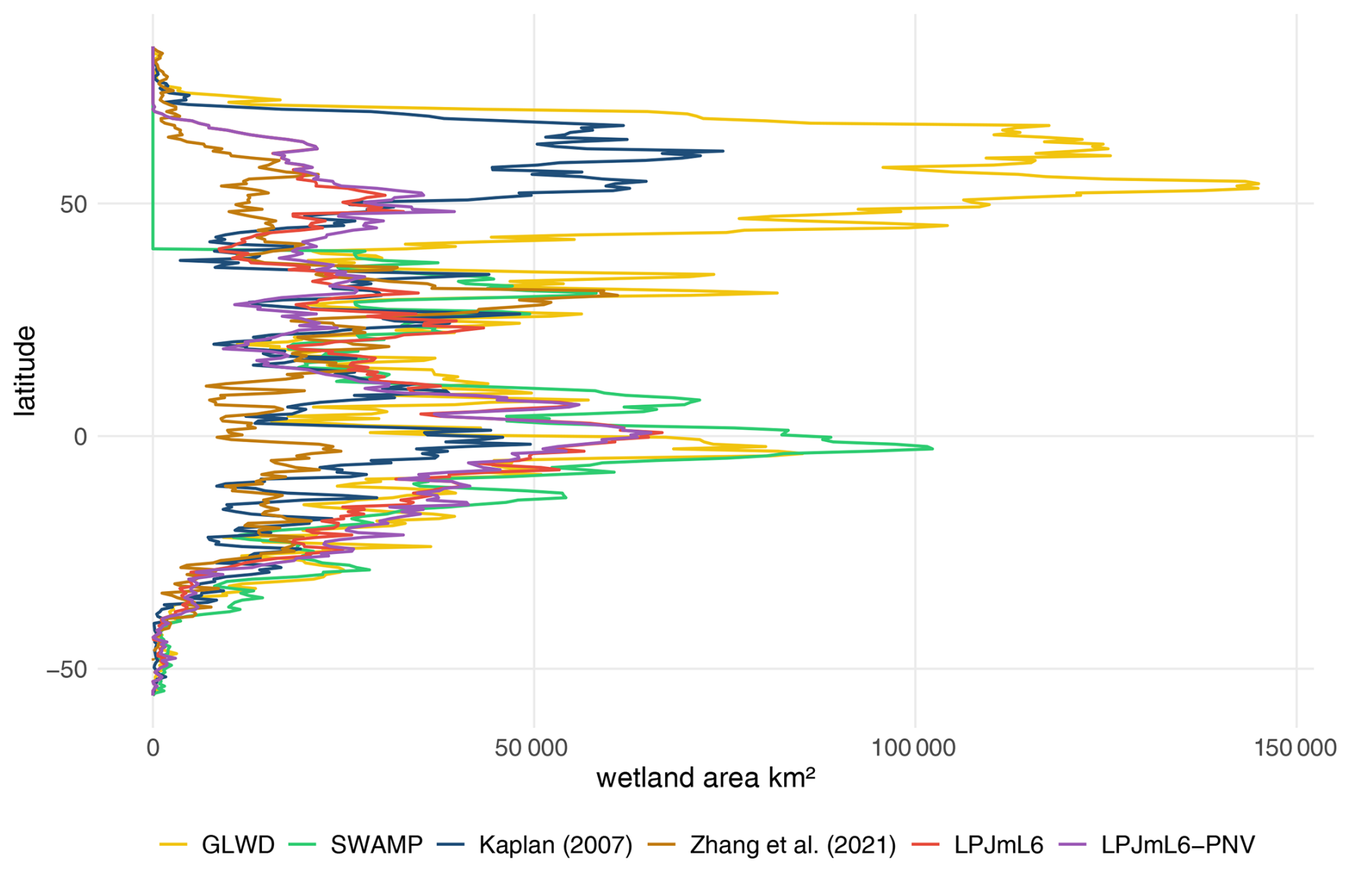
Figure 3 Latitudinal distribution of zonal wetland area from different data products and from LPJmL6 (with land-use change) and LPJmL6–PNV (potential natural vegetation). Wetland area is integrated along longitude for each half degree latitude band (km²).

5.3 Methane budget

In this section, we confront the land CH₄ budget simulated by LPJmL6 with independent constraints on the global CH₄ budget. The global budget is determined by the balance between all surface sources and atmospheric sinks of CH₄ and is constrained by the observed atmospheric CH₄ burden, its temporal growth and estimates of the atmospheric CH₄ lifetime (Stevenson et al., 2020; Saunois et al., 2020; He et al., 2021; Saunois et al., 2025). These constraints define a range of total CH₄ emissions and, by subtraction of quantified source categories, a residual range attributable to net land sources.

LPJmL6 represents a subset of the global CH₄ cycle, namely emissions from natural wetlands, rice cultivation, wildfires and other agricultural soils, as well as aerobic soil CH₄ uptake. We refer to the sum of these components (emissions minus soil uptake) as the LPJmL6 land CH₄ budget. To relate this modelled land budget to the global CH₄ budget, we combine LPJmL6 fluxes with independent estimates of other anthropogenic and natural sources that are not simulated by LPJmL6 (enteric fermentation and manure management, landfills and waste, fossil fuel-related emissions, biomass and biofuel burning, and additional natural sources). This allows a consistent comparison of LPJmL6 with bottom-up (BU) and top-down (TD) global estimates and with the lifetime-based constraints on total emissions.

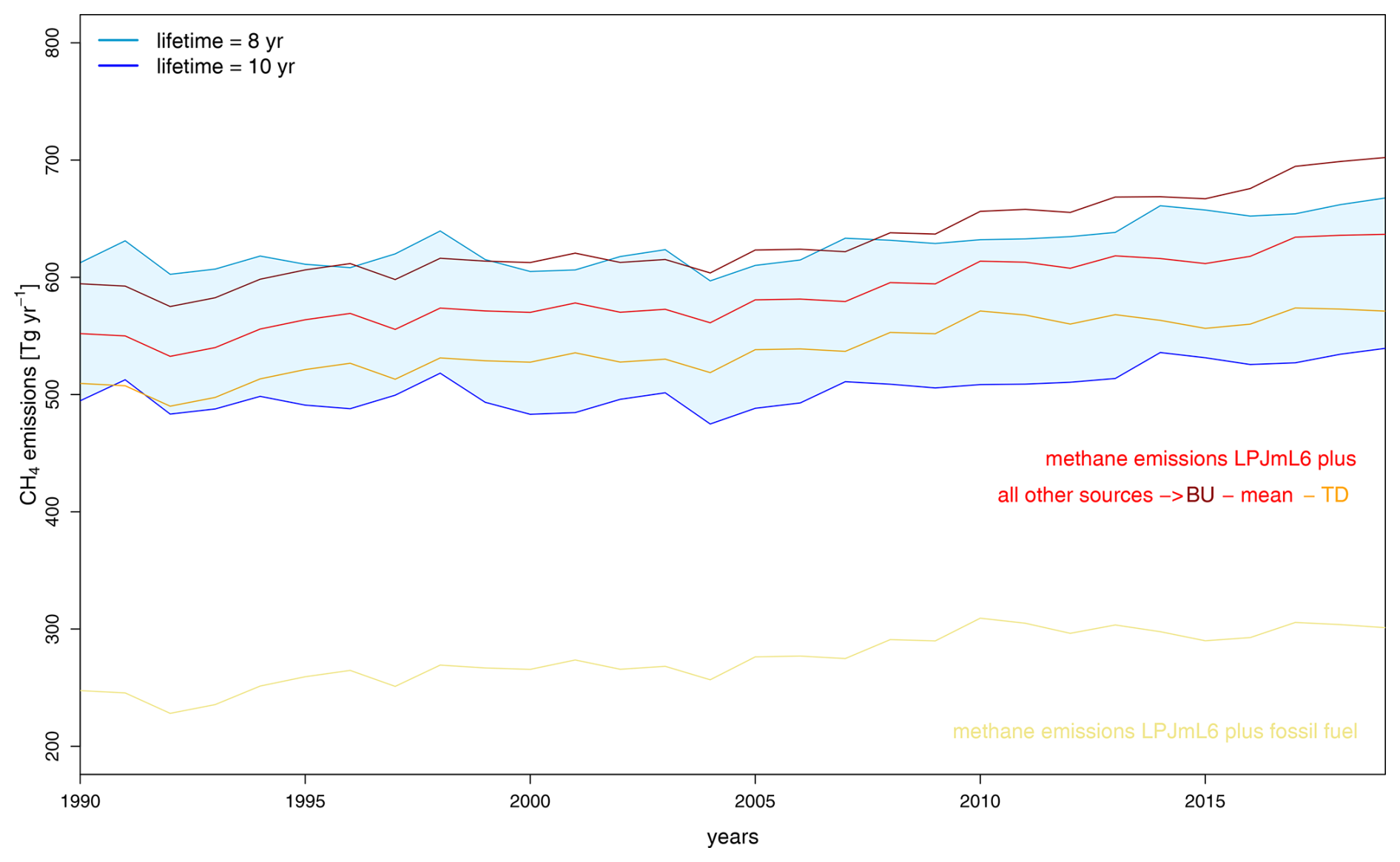
Figure 4 Global methane budget calculated from the atmospheric methane concentration and estimated lifetime of methane and the atmospheric growth resulting in the estimated overall methane sink that gives the range of the assumed methane emissions. Methane sources are anthropogenic (enteric fermentation& manure, landfills & waste, biomass & biofuel burning) and natural (incl. freshwater, geological, wildfires, termites, oceanic) (Saunois et al., 2025) and the range of the atmospheric methane lifetime is given by Stevenson et al. (2020). The two blue lines (labelled lifetime = 8 years and lifetime = 10 years) and the blue shaded area between them represent the atmospheric constraint, indicating the range of total global methane emissions, i.e. the region in which the sum of all sources and the soil sink should lie for a closed global methane budget. Bottom-up (BU) and top-down (TD) estimates, given as decadal means for 2000–2009 and 2010–2019, are converted to continuous annual values by linear interpolation between these two means; the resulting BU and TD time series are added to the simulated LPJmL6 methane sources and define the range shown by the orange and dark red lines. LPJmL6 simulated net methane sources include emissions from wetlands, rice cultivation, and wildfires and the soil sink.

5.3.1 Methane emissions

The global constraints on CH₄ sources and sinks outlined above allow a more detailed comparison of LPJmL6-simulated emissions with other global estimates. LPJmL6 simulates CH₄ emissions from wetlands, rice fields, and wildfires, and can distinguish between emissions from agricultural land and natural land. Furthermore, LPJmL6 explicitly represents soil CH₄ uptake via diffusion from the atmosphere into the soil. To derive the possible range of CH₄ emissions compatible with observations, source categories that are not explicitly calculated by LPJmL6 have to be added. These include anthropogenic emissions from enteric fermentation and manure management, and from landfills and waste (about 170–205 TgCH₄ a⁻¹), as well as fossil fuel–related emissions (about 145 TgCH₄ a⁻¹) (NOAA Global Monitoring Laboratory, 2025) and biomass combustion (about 28 TgCH₄ a⁻¹). Together, these account for 462–481 TgCH₄ a⁻¹ (Saunois et al., 2025, 2020; Li et al., 2021; Stanley et al., 2016). Additional natural sources not represented in LPJmL6, such as emissions from freshwater systems, geological sources, termites and the ocean, account for a further 64–259 TgCH₄ a⁻¹, with particularly large uncertainty for freshwater emissions. For the illustrative period 2010–2019, the atmospheric CH₄ sink is estimated to be between 523 and 649 TgCH₄ a⁻¹.

Depending on the estimated CH₄ lifetime in the atmosphere given by Stevenson et al. (2020), between 31 and 242 TgCH₄ a⁻¹ remain attributable to land net sources, for which LPJmL6 simulates about 142.1 TgCH₄ a⁻¹ (wetlands, fire, rice cultivation, and other agricultural soil emissions and the explicitly simulated soil sink; mean over the years 2000 to 2019; see Table 3). If, however, we enforce global budget consistency by combining the lower (upper) estimates of the atmospheric sink with the lower (upper) estimates of CH₄ sources not simulated by LPJmL6, the residual range attributable to land net sources narrows to 116–157 TgCH₄ a⁻¹, which still encompasses the LPJmL6 estimate (see Fig. 4).

When all emissions simulated by LPJmL6 are combined with estimates for the remaining anthropogenic and natural sources, the resulting overall CH₄ budget matches well with the observationally constrained overall emissions Fig. 4. We construct two such combined estimates: one using bottom-up (BU) values for the non-LPJmL sources and one using top-down (TD) values. Adding the same LPJmL6 land emissions to these two source data sets shifts both curves upwards by the modelled land flux; in our set-up this makes the BU-based combination systematically higher and the TD-based combination lower. Consequently, the BU+LPJmL6 series forms the upper envelope and the TD+LPJmL6 series the lower envelope of the total-budget range shown by the red and orange lines in Fig. 4, respectively.

Table 2 summarizes CH₄ emissions from wetlands as estimated by the Global Methane Budget project (Kirschke et al., 2013; Saunois et al., 2016, 2020, 2025). For the period 2000–2009, BU estimates range between 147 and 175 TgCH₄ a⁻¹, whereas TD estimates range from 180 to 217 TgCH₄ a⁻¹. The discrepancy between these methodologies is evident across all decades examined. Notably, the differences are largest in the 1980s and 1990s, exceeding 50 TgCH₄ a⁻¹. MOre recent estimates show reduced discrepancies, with TD estimates decreasing significantly while BU estimates remain relatively stable. LPJmL6 aligns closely with BU estimates, reflecting its process-based methodology and explicit integration of wetland hydrology.

Kirschke et al. (2013)Saunois et al. (2016)Saunois et al. (2020)Saunois et al. (2025)

Table 2 Global methane emissions in TgCH₄ a⁻¹ from natural wetlands across four decades, presenting values separately for bottom-up (BU) and top-down (TD) methods. The variation reflects the methodological differences and uncertainties in emission processes.

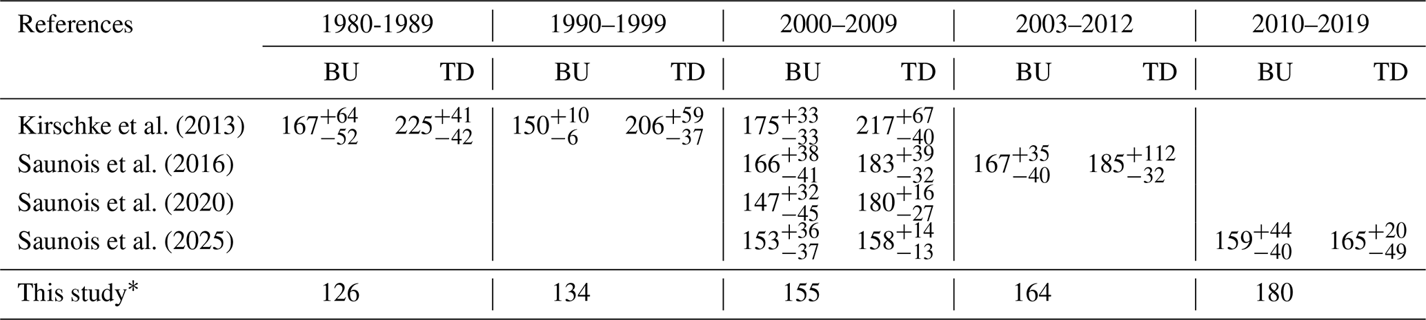
^* here we report data from the simulation with actual vegetation, but exclude emissions from rice fields for consistency with the reference data

The site-level comparison, shown in the Supplement (Figs. S5–S21), indicates that LPJmL6 reproduces the observed seasonal and cumulative CH₄ emissions at some sites, for example RU–Ch2, US–Tw1, and US–Myb, but performs less well at others. This behaviour is expected because eddy-covariance CH₄ measurements often represent relatively small and heterogeneous source areas, whereas LPJmL6 simulates grid-cell mean fluxes. Individual tower footprints may therefore be dominated by local wetland patches, drainage features, vegetation composition, management, or water-table dynamics that are not representative of the corresponding 0.5° grid cell. Consequently, mismatches at individual sites do not necessarily indicate a failure of the large-scale model process representation, but may reflect a scale mismatch between local observations and grid-cell averages.

The cumulative comparison is often more robust than the month-to-month comparison because it integrates over short-term variability and gaps in the observations. However, the FLUXNET-CH₄ records are frequently incomplete, and missing periods can affect both monthly sums and cumulative totals, especially when data gaps occur during peak emission periods. Therefore, the site-level evaluation should mainly be interpreted as a diagnostic of seasonal timing and order-of-magnitude agreement, rather than as a strict validation of local flux magnitudes at every site.

Figure 5 compares the spatial and latitudinal distribution of wetland CH₄ emissions simulated by LPJmL6 with the WetCHARTs ensemble (Bloom et al., 2017b). Both data sets show a pronounced tropical maximum in the latitudinal profile, reflecting the dominant contribution of tropical wetlands to the global wetland CH₄ emissions. In terms of zonally summed emissions, LPJmL6 agrees reasonably well with the WetCHARTs ensemble median across broad latitude bands and remains mostly within the WetCHARTs min–max range, particularly outside the tropical peak region.

However, the spatial comparison indicates that similar latitudinal totals can arise from different regional emission patterns. The anomaly map shows regional offsets between LPJmL6 and the WetCHARTs median, including areas where LPJmL6 underestimates or overestimates emissions relative to WetCHARTs despite comparable zonal sums. This suggests that agreement in the latitudinal profile should not be interpreted as full spatial agreement. Part of this mismatch is expected because the comparison is made only against the WetCHARTs ensemble median, while the ensemble spread reflects substantial uncertainty in wetland extent and CH₄ flux estimates. In addition, LPJmL6 is run on a coarse spatial grid and does not explicitly represent bank infiltration or river–floodplain exchange processes, which limits its ability to resolve narrow floodplains, riparian wetlands, and seasonal inundation features that can contribute substantially to local CH₄ emissions.

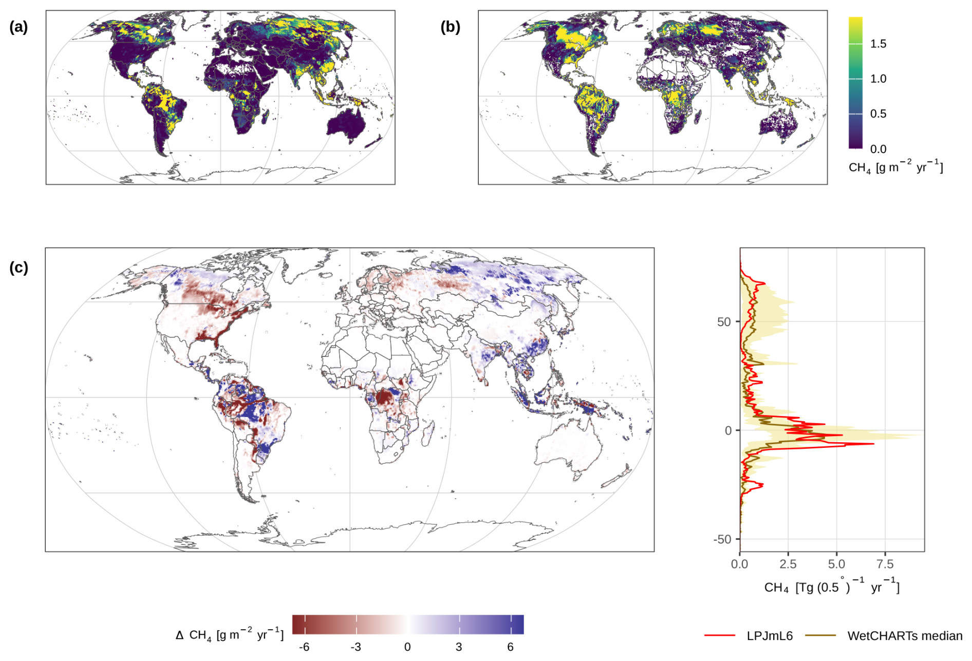
Figure 5 Spatial and latitudinal comparison of wetland CH₄ emissions simulated by LPJmL6 with the WetCHARTs ensemble (Bloom et al., 2017b). Maps show (a) LPJmL6 wetland CH₄ emissions, (b) the WetCHARTs ensemble median, and (c) the anomaly between LPJmL6 and WetCHARTs, calculated as LPJmL6 minus the WetCHARTs median. Map values are shown as annual flux densities in g CH₄ m⁻² a⁻¹. The latitudinal profile shows area-weighted zonal sums in Tg CH₄ (0.5°)⁻¹ a⁻¹. The WetCHARTs min–max range is shown as a shaded band, and the ensemble median is shown as a solid line.

5.3.2 Methane emissions from the different flux components

Quantifying the exact global contribution of each pathway is challenging because of spatial and temporal variability in wetland extent, hydrology and vegetation, as well as differences in wetland types and environmental conditions. Table 3 therefore summarises the LPJmL6 global methane budget separated into atmospheric flux pathways (diffusion, plant-mediated transport, ebullition and fire emissions) and source categories (natural wetlands, rice fields, grasslands and other cropland), together with soil oxidation and the resulting net methane sink. This pathway- and source-resolved budget provides a process-level decomposition of the simulated CH₄ emissions and complements the spatial evaluation against WetCHARTs. It allows the relative importance of the main atmospheric transport pathways to be assessed separately from the contributions of different land-use and wetland source categories. In this way, the table provides an additional diagnostic for interpreting the model behaviour beyond the total wetland CH₄ flux and the latitudinal emission patterns.

Table 3 LPJmL6 estimates of global methane balance differentiated for different components in TgCH₄ a⁻¹.

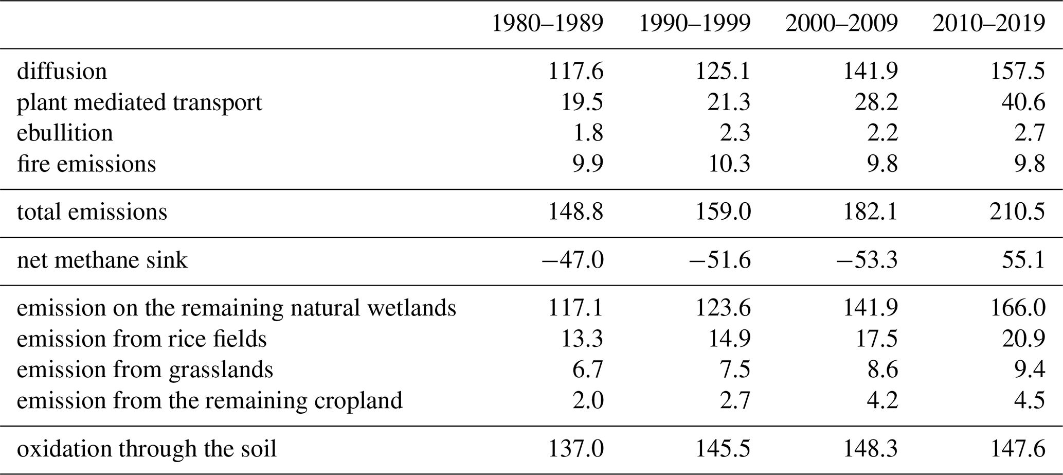
The atmospheric flux partitioning shows that diffusion remains by far the dominant CH₄ emission pathway, with global emissions increasing from 117.6 to 157.5 Tg CH₄ a⁻¹ between the 1980s and 2010–2019. Plant-mediated transport roughly doubles from 19.5 to 40.6 Tg CH₄ a⁻¹ over the same period, whereas ebullition remains comparatively small (about 2 Tg CH₄ a⁻¹) and exhibits no clear trend, in line with the minor contribution of ebullition reported by Bieniada and Strack (2021). Fire emissions are simulated at around 10 Tg CH₄ a⁻¹, consistent with independent estimates of global wildfire CH₄ emissions of approximately 10 Tg CH₄ a⁻¹ and contributing about 5 % of the total natural source (Saunois et al., 2025).

The soil methane sink in LPJmL6 can be compared with independent constraints. Murguia-Flores et al. (2018) estimated a global soil CH₄ sink of 33.5 Tg CH₄ a⁻¹ for 1990–2009, whereas LPJmL6 simulates a stronger net uptake of about 52 Tg CH₄ a⁻¹ over the same period (Table 3). A key difference is that LPJmL6 does not explicitly represent the atmospheric CH₄ sink associated with methanotrophic activity in well-aerated soils; instead, CH₄ oxidation is treated as part of the soil CH₄ balance. The gross soil oxidation flux in LPJmL6 is close to 150 Tg CH₄ a⁻¹, reflecting the substantial fraction of CH₄ that is oxidized while diffusing through the unsaturated zone. Despite these structural differences, the simulated net soil sink lies within, albeit towards the upper end of, the range of 9–51 Tg CH₄ a⁻¹ reported by atmospheric inversions and bottom-up estimates (Saunois et al., 2025).

Because LPJmL6 explicitly represents both natural and managed ecosystems, including land use and land-use change, it can attribute global CH₄ emissions to distinct source categories. In our simulations, emissions from natural wetlands increase from 117 to 166 Tg CH₄ a⁻¹ between the 1980s and 2010–2019, while emissions from rice fields rise from 13.3 to 20.9 Tg CH₄ a⁻¹. This corresponds to an increase of about 57 % in rice-field emissions compared to only about 13 % growth in harvested rice area. Emissions from other agricultural land (excluding rice and grasslands) grow from 2.0 to 4.5 Tg CH₄ a⁻¹, and grassland emissions from 6.7 to 9.4 Tg CH₄ a⁻¹. For comparison, EPA (2012) estimated that other agricultural CH₄ sources contribute roughly 20 Tg CH₄ a⁻¹ for 2005–2020, which is higher than the LPJmL6 estimate but broadly consistent when considering that the EPA category also includes savanna and residue burning. Overall, all simulated source categories exhibit increasing CH₄ emissions over recent decades, likely reflecting the combined effects of climate change and evolving land management; however, the relative contributions of these drivers warrant further investigation.

Another important aspect of LPJmL6 is the explicit representation of both natural and managed ecosystems, including land-use and land-use change dynamics. This structure allows us to attribute simulated changes in global CH₄ emissions to distinct source categories and regions across the terrestrial surface and to link emerging trends to underlying drivers. Such source-resolved information is essential for understanding, and ultimately mitigating, the role of wetlands and agricultural systems in global greenhouse gas budgets. The LPJmL6 model allows us to separately quantify global CH₄ emissions from natural wetlands, rice fields, grasslands and other agricultural land. In the simulations, emissions from natural wetlands increase from 117 Tg CH₄ a⁻¹ in the 1980s to 166 Tg CH₄ a⁻¹ in 2010–2019. Emissions from rice fields rise from 13.3 to 20.9 Tg CH₄ a⁻¹ over the same period, corresponding to an increase of about 57 %, whereas harvested rice area increases by only about 13 %. Emissions from other agricultural land (excluding rice and grasslands) grow from 2.0 to 4.5 Tg CH₄ a⁻¹, and grassland emissions from 6.7 to 9.4 Tg CH₄ a⁻¹. Over the same period, simulated global grassland area increases by only about 5 %, implying that the roughly 40 % rise in grassland CH₄ emissions is driven primarily by changing environmental conditions and management rather than by areal expansion alone. For comparison, EPA (2012) estimated that other agricultural CH₄ sources contribute roughly 20 Tg CH₄ a⁻¹ for 2005–2020, which is higher than the LPJmL6 estimate but broadly consistent when considering that the EPA category also includes savanna and residue burning. Overall, all simulated source categories exhibit increasing CH₄ emissions over recent decades, consistent with the combined effects of changing climate conditions and evolving agricultural practices; however, the relative contributions of these drivers require further investigation.

5.3.3 Emission from rice cultivation, grasslands and other agricultural land

Table 4 summarizes literature estimates of global CH₄ emissions from rice cultivation, aggregated over the growing seasons, together with the corresponding LPJmL6 simulations. Most literature values are multi-year means for the period indicated in the table (rather than single-year snapshots). They are based on a range of methodological approaches, including emission-factor inventories, statistical upscaling from field measurements, and FAOSTAT-based accounting, and span roughly 18.3 to 38.8 TgCH₄ a⁻¹. LPJmL6 simulates an increase from a global mean of 13.0 TgCH₄ a⁻¹ in the 1980s to 20.4 TgCH₄ a⁻¹ during 2010–2019, which places our results toward the lower end of the published range (Table 4). A likely explanation is that the current representation of rice production systems assumes one cropping season per grid cell, whereas multi-cropping (double or even triple rice) is widespread in parts of South and Southeast Asia and eastern China (Waha et al., 2025, 2020). In such regions, annual emissions exceed the values simulated by LPJmL6 because emissions from multiple growing seasons within a calendar year are not explicitly represented. In annual sums of LPJmL6 simulated emissions, we combine planted rice area with those from wetland-setaside emissions on these fields, which captures major biogeochemical controls but may still under-represent management effects such as straw incorporation, organic amendments, and deliberate drainage. In the LPJmL6 simulations, the unproductive (non-growing) period contributes about 4 TgCH₄ a⁻¹. While the emission estimates obtained with other methodologies are strongly influenced by how the contributing days are defined, the very wide range of 8–78 Tg CH₄ a⁻¹ simulated by by the process-based model CH4MOD (Hu et al., 2024) is mainly driven by differing assumptions about management.

Yan et al. (2009)Hu et al. (2024)Pazhanivelan et al. (2024)FAO (2020c)EPA (2012)Wang et al. (2023a)Saunois et al. (2025)

Table 4 Global CH₄ emissions from rice cultivation during the growing season.

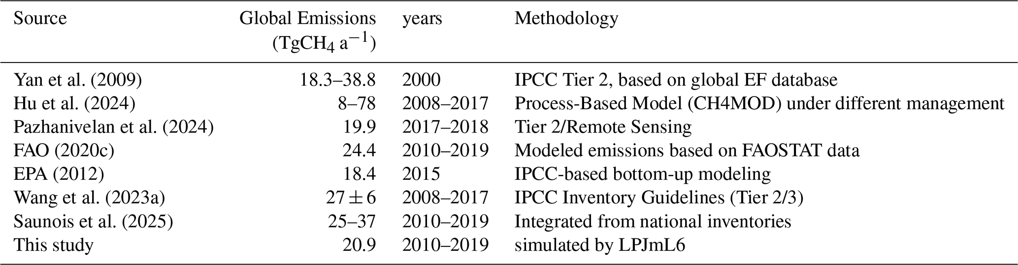
Table 5 Country-level cumulative CH₄ emissions from rice fields during the growing season simulated by LPJmL6 (1990–2014 mean, gCH₄ m⁻² a⁻¹). For each country, the table reports the mean, minimum, and maximum emissions within the national rice area.

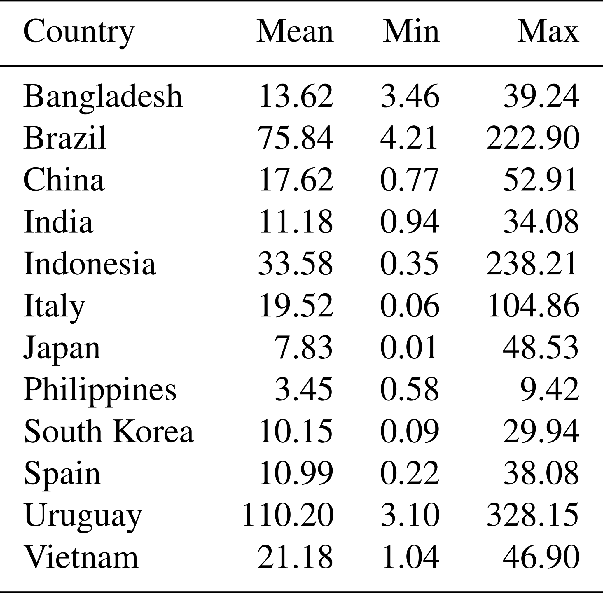
Across rice-growing regions, methane emissions from rice fields exhibit strong spatial and temporal variability. LPJmL6 simulates country-mean cumulative growing-season emissions that range from a few to more than 100 gCH₄ m⁻² a⁻¹, with local grid-cell values reaching up to 328 gCH₄ m⁻² a⁻¹ in the most strongly emitting areas (Table 5). The observed values compiled in Table 6 span a comparable order of magnitude, with maximum values extending from about 13 up to 347.5 gCH₄ m⁻² a⁻¹, indicating pronounced sub-national heterogeneity within the sampled regions. Independent field studies further highlight the very strong variability of rice CH₄ emissions. Wang et al. (2022) report substantial year-to-year differences in growing-season emissions from Chinese rice fields, with high emissions of 36.8 gCH₄ m⁻² a⁻¹ in 2018 and low emissions of 5.3 gCH₄ m⁻² a⁻¹ in 2019, while Qian et al. (2023) document even higher plot-scale values approaching 580 gCH₄ m⁻² a⁻¹ under specific conditions, illustrating the potential for extreme fluxes in certain regions or management settings. It is important to note that LPJmL6 always provides spatially complete coverage of each national rice area, whereas most literature values in Table 6 are derived from individual sites or sub-regions and therefore cannot be interpreted as true national means, even in the comparatively extensive dataset of Wang et al. (2018). This mismatch in spatial representativeness, together with differences in local management practices, environmental conditions and measurement protocols, explains part of the discrepancies between simulated and observed ranges, while the overall overlap in magnitude supports the ability of LPJmL6 to capture first-order patterns of rice CH₄ emissions.

Wang et al. (2018)Zhu and Li (2024)Wang et al. (2018)Wang et al. (2018)Wang et al. (2018)Gupta et al. (2021)Bhatia (2013)Wang et al. (2018)Wang et al. (2018)Wassmann et al. (2000)Wang et al. (2018)Wang et al. (2018)Wang et al. (2018)Wang et al. (2018)Wang et al. (2018)Wang et al. (2018)

Table 6 Observed cumulative CH₄ emissions from rice fields during the rice-growing season (gCH₄ m⁻² a⁻¹), compiled from field studies and grouped by region. Reported minimum and maximum values denote the lowest and highest growing-season emissions observed across the years covered in each study.

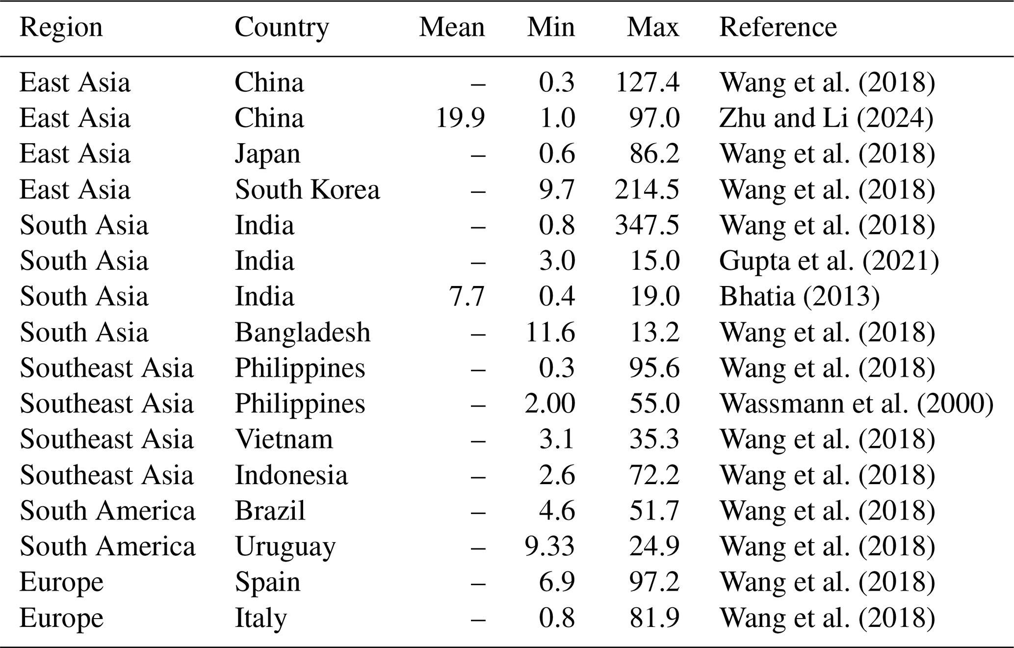
Globally, grasslands exhibit simulated CH₄ emissions that are half those from rice paddies, as indicated in Table 3. This important source of CH₄ emissions arises from two primary factors. First, the vast spatial extent of grasslands worldwide provides a substantial area for CH₄ production and emission, despite the generally lower CH₄ fluxes per unit area compared to rice paddies. Second, many grassland regions, particularly those converted from historical peatlands, are characterized by drained organic soils. The drainage of these former peatlands for agricultural use not only alters the hydrological regime but also influences the soil carbon dynamics, creating conditions conducive to CH₄ emissions (van den Pol-van Dasselaar, 1998). Residual croplands constitute a small but non-zero CH₄ source that is highly sensitive to field-scale hydrology. Even in nominally aerated systems, shallow or perched water tables, episodic waterlogging after irrigation or storms, and poorly drained depressions can create anoxic microsites where methanogenesis occurs. The resulting emissions are intermittent and heterogeneous, governed primarily by water-table depth and inundation frequency. Although flux magnitudes are typically far lower than those from wetlands, such emissions can be regionally relevant in poorly drained landscapes and in wet seasons, and they carry high spatial and interannual variability.

5.4 Carbon pools and fluxes

The implementation of the anoxic decomposition also influences the organic carbon pools and the CO₂ fluxes into the atmosphere. Therefore the LPJmL6 model needs to be benchmarked for the other important carbon cycle variables as well.

5.4.1 Net biome production

The release of soil carbon is decelerated due to the representation of wetlands in the LPJmL6 models. The anoxic decomposition is about 10 times slower and thus carbon is sequestered in soils for a much longer time. Thus the model can well reproduce the magnitude of the global carbon sink – including land-use change (LUC) emissions – within the estimate range of the Global Carbon Budget (GCB) 2023 (Friedlingstein et al., 2023) from Dynamic Global Vegetation Models (DGVM) and from the bookkeeping approach (DGVM-LU-BK) (see Table 7 and Fig. 6). Table 7 shows that LPJmL6 reproduces decadal terrestrial sink magnitudes within the GCB 2023 DGVM and DGVM-LU-BK uncertainty ranges and exhibits the expected strengthening from the 1990s to the 2010s; across the two GCB methods, residual differences can be traced to land-use-change treatment – bookkeeping versus implicit DGVM dynamics – and no systematic decadal bias is evident; this also holds for LPJmL6, indicating robust, method-invariant trends in the net land carbon sink. In Fig. 6, the simulated terrestrial sink follows the independently constrained apparent sink and the atmospheric CO₂ growth rate with comparable interannual variability, indicating that LPJmL6 captures the major climate-driven fluctuations and the multi-decadal increase in sink strength without long-term divergence from independent estimates.

Table 7 Net biome production-Terrestrial land sink including land use change emissions estimated by Global Carbon Budget 2023 and simulated by LPJmL6.

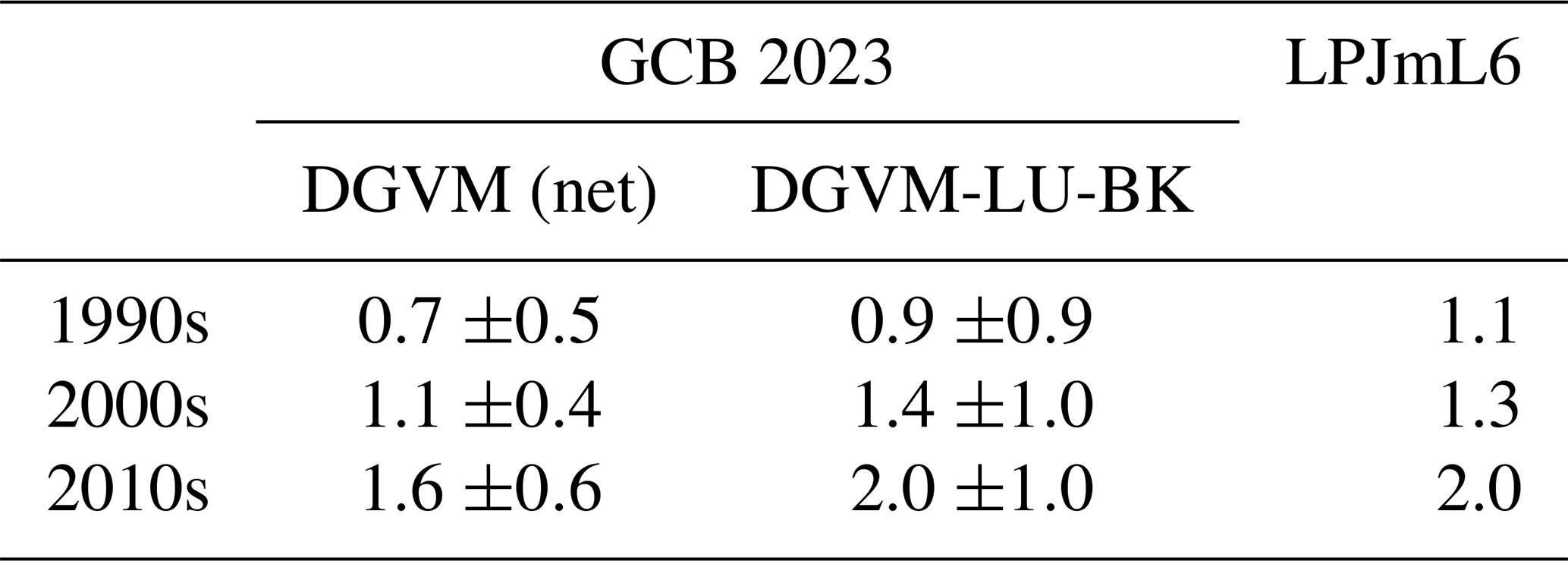
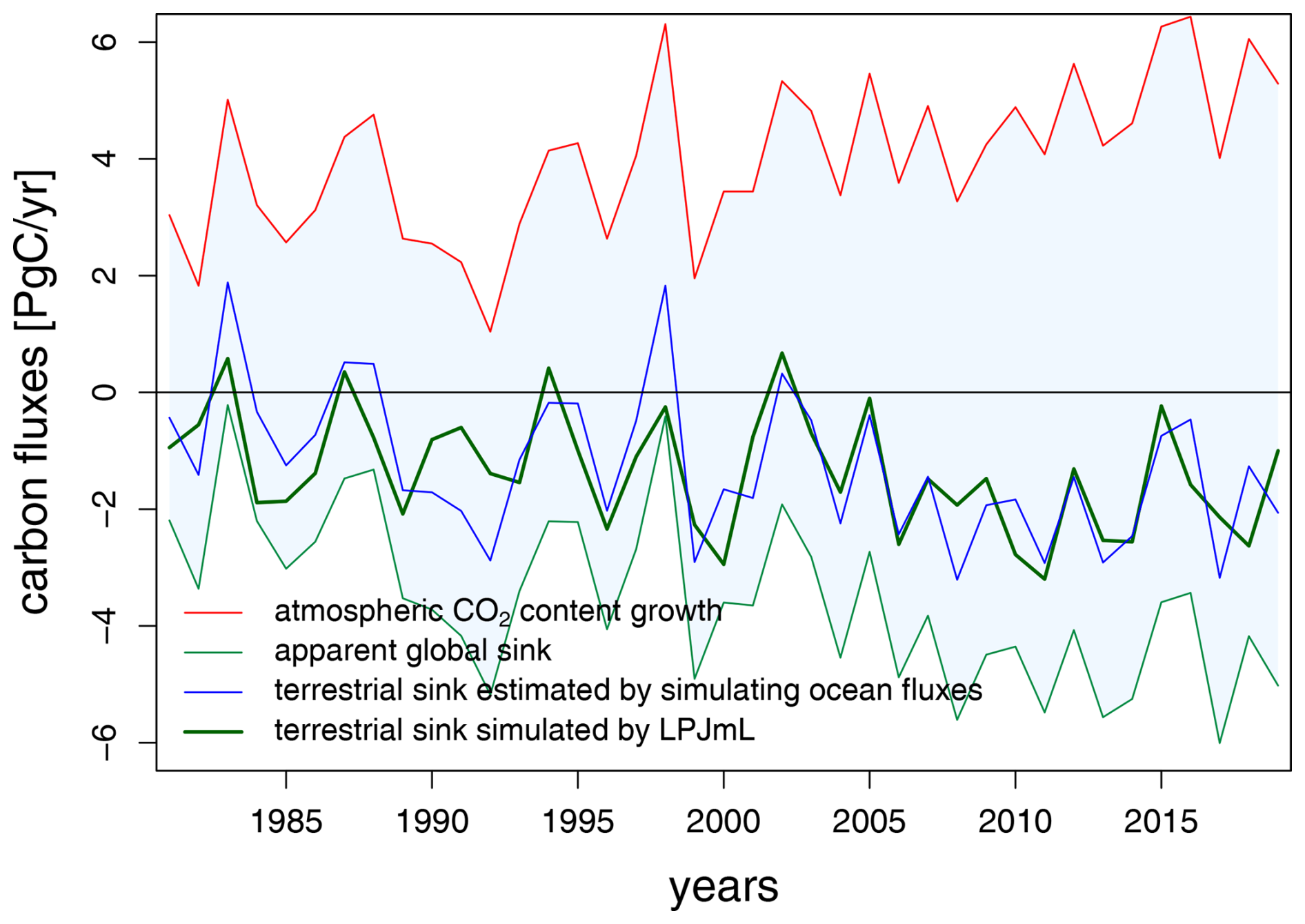
Figure 6 Terrestrial sink estimated by LPJmL6 and Global Carbon Budget 2023 (Friedlingstein et al., 2023).

5.4.2 Net ecosystem exchange

We used eddy-covariance flux tower data to benchmark simulated NEE (Fig. 7; full data description in Sect. 4.2). As noted there, comparisons are constrained by scale mismatches between grid cells and tower footprints, possible vegetation (PFT) mismatches, and the use of large-scale meteorological forcing rather than site-specific observations, which limits the ability to capture site-specific variability in carbon fluxes.

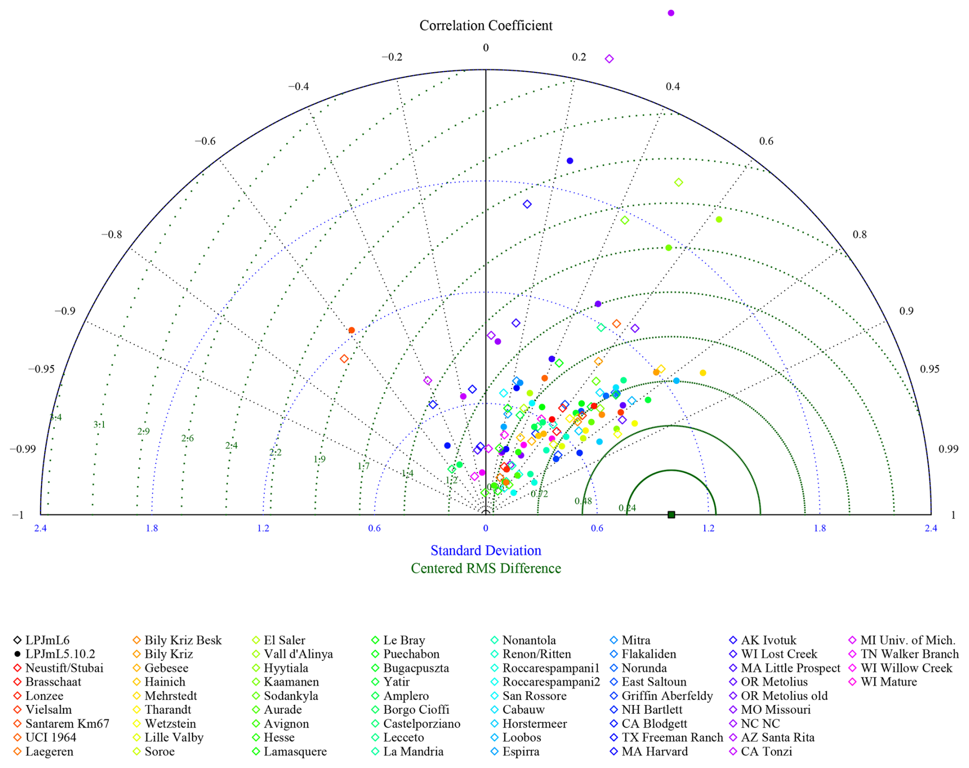
Figure 7 Taylor diagram showing the comparison of simulated net ecosystem exchange (NEE) against eddy-covariance flux tower measurements. Observational data are derived from the FLUXNET network, which provides standardized eddy-covariance measurements of ecosystem–atmosphere carbon and water fluxes (Pastorello et al., 2020).

Nevertheless, the comparison demonstrates that correlations between simulated and observed fluxes are generally high across many sites, indicating that the model captures the overall temporal dynamics of NEE reasonably well. However, the centered root mean square difference (CRMSD) and the normalized standard deviation reveal larger discrepancies, suggesting that while the timing of seasonal and interannual variability is reproduced, the magnitude of fluxes is often either over- or underestimated.

5.4.3 GPP

The ILAMB comparison demonstrates that the model successfully reproduces gross primary production (GPP) within the same order of magnitude as reported by Jung et al. (2011) (global mean 119 ± 6 PgC a⁻¹ for 1982–2008 vs. 126 PgC a⁻¹ simulated by LPJmL6). This agreement is also in line with later FLUXCOM syntheses that place global GPP roughly in the 106–130 PgC a⁻¹ range, depending on predictors and machine-learning methods used (Jung et al., 2020).

5.4.4 Aboveground biomass (AGB)

Across the ILAMB benchmark, reference biomass products differ in scope (forest AGB vs. all vegetation; above- vs. below-ground components), spatial/temporal coverage, and retrieval/inversion methodology, yielding a wide spread in implied global stocks. LPJmL6 estimates global woody biomass to be 422 PgC (mean 2000–2019). Among reference datasets, products that resolve high biomass in humid tropical and high-latitude forests report totals comparable to LPJmL6, for example, GEOCARBON 408 PgC (GEO, 2014); the Xu–Saatchi synthesis 381 ± 2 PgC for 2000–2019 (Xu et al., 2021). By contrast, ESA CCI Biomass provides forest AGB of 300 PgC (above-ground forest only) (GEO, 2014; Santoro et al., 2021), and NBCD2000 is regional (conterminous U.S., sim∼2000 baseline), serving primarily for spatial pattern evaluation rather than global sums (Kellndorfer et al., 2012). These definitional and methodological contrasts account for the spread in ILAMB intercomparisons and explain why LPJmL6 aligns more closely with datasets emphasizing woody stocks across humid tropical and boreal forests, whereas ESA CCI implies lower global totals.

From the reference data sets used in ILAMB, only the Xu–Saatchi (Xu et al., 2021) product (381 PgC) aligns closely with the LPJmL6 simulation result of 422 PgC, whereas most other datasets imply substantially higher global biomass totals ranging from 300 to 408 PgC.

5.5 Water fluxes

We assess the large-scale terrestrial water cycle to ensure that the CH₄ implementation operates within a physically consistent land-surface framework. The analysis combines global budgets with spatial diagnostics (renewable water resources and groundwater recharge) and skill metrics for multi-decadal river discharge and evapotranspiration (ET) simulations.

5.5.1 Global water fluxes

Table 8 synthesizes ranges of data-driven and model-based estimates for the principal terrestrial water fluxes – evapotranspiration (ET), transpiration (T), total runoff from land, groundwater recharge, and irrigation withdrawals. ET (62×10³ km³ a⁻¹) and T (39×10³ km³ a⁻¹) fall within published model ranges and are near the lower bounds of data-driven syntheses, indicating a conservative global partitioning of ET. Total runoff and river discharge (47 and 40×10³ km³ a⁻¹) lie near the centers of reported ranges, consistent with independent constraints. Groundwater recharge (31×10³ km³ a⁻¹) exceeds data-driven and modeled estimates; this difference reflects varying definitions (diffuse vs. focused recharge and return flows), considered land areas, and averaging periods, also examined spatially in Sect. 5.5.2, with discharge and ET evaluations provided in Sect. 5.5.3 and 5.5.4. Nevertheless, the LPJmL6 estimate is near the upper end of published values and coincides with greater groundwater storage in the simulations than reported Müller Schmied et al. (2021) (Fig. 8).

Table 8 Simulated global terrestrial water fluxes, and ranges of data-driven and modeled estimates (in 10³ km³ a⁻¹). Evapotranspiration and transpiration represent long-term land averages (1982–2011); runoff and discharge are multi-decadal climatologies (1982–2011 land means); infiltration denotes diffuse groundwater recharge; irrigation withdrawals (around 2010) include both surface and groundwater abstraction.

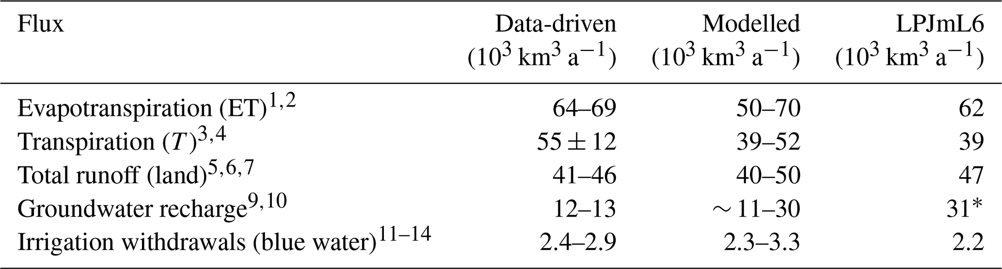
References:¹ Pan et al. (2020); ² Wild et al. (2015); ³ Jasechko et al. (2013); ⁴ Good et al. (2015); ⁵ Schneider et al. (2017); ⁶ Godoy et al. (2021); ⁷ Döll et al. (2016); ⁸ Mohan et al. (2018); ⁹ Döll and Fiedler (2008); ¹⁰ FAO (2020a); ¹¹ Wada and Bierkens (2014); ¹² Wada et al. (2014); ¹³ Huang et al. (2018); ¹⁴ FAO (2020a); ^* including return flows from irrigation

5.5.2 Groundwater recharge and renewable storage

Figure 8 compares long-term mean groundwater storage (GWS) and groundwater recharge for 1981–2010 from WaterGAP 2.2 (Müller Schmied et al., 2021) and LPJmL6. Recharge is highest in humid tropics and monsoon regions (Amazon, Congo, SE Asia, eastern India), and is moderate in temperate wet zones, and near zero across arid belts (Sahara, Arabian Peninsula, central Australia); orographic bands (Andes, Himalaya) are evident. Storage broadly tracks persistently wet lowlands and large sedimentary basins, with minima in deserts and high-latitude regions. LPJmL6 tends to display sharper spatial gradients and stronger orographic signals, while WaterGap is smoother and often more conservative in semi-arid interiors.

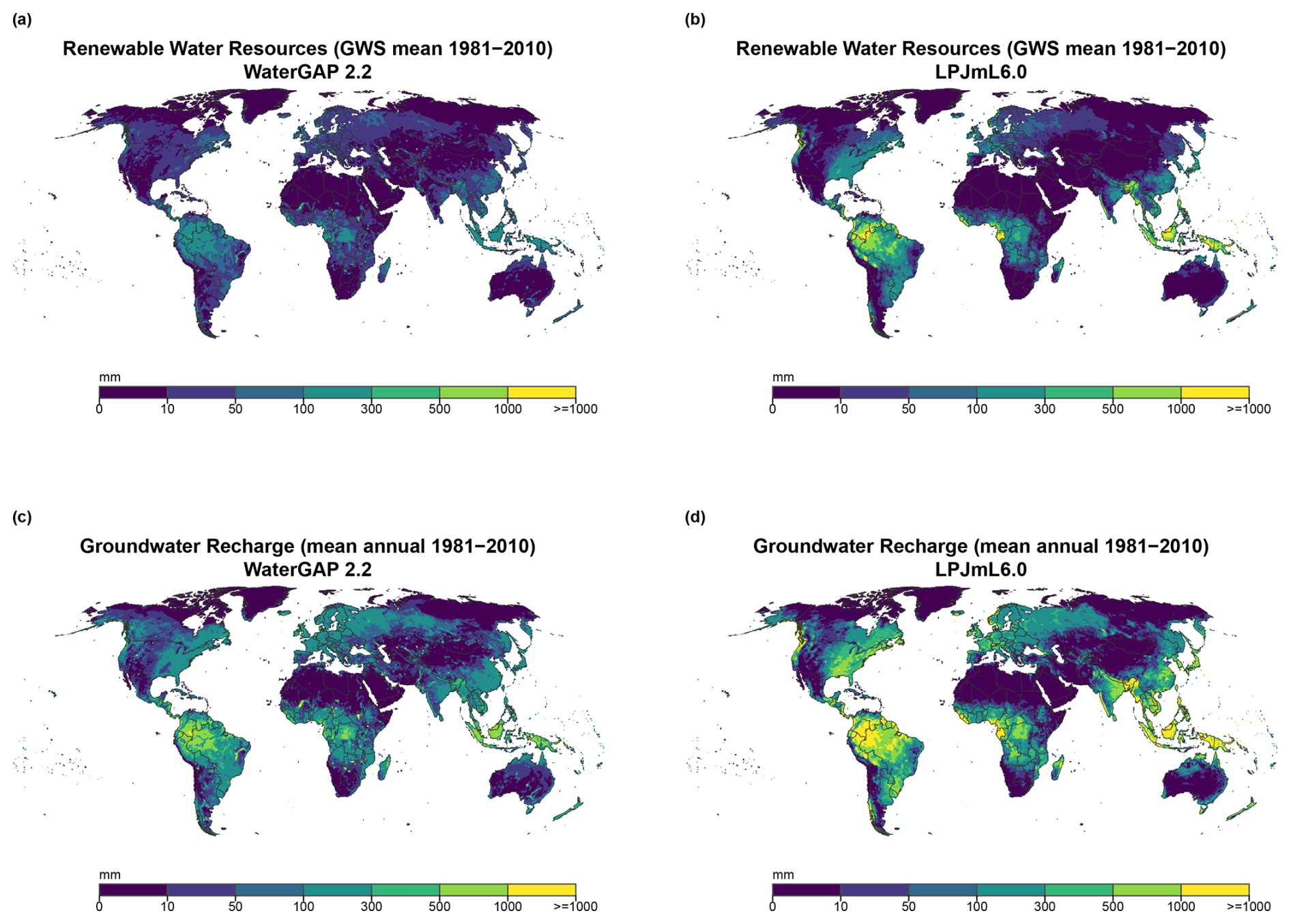
Figure 8 Comparison of WaterGAP 2.2 (Müller Schmied et al., 2021) and LPJmL6 maps of (a, b) renewable groundwater storage (GWS; multi-year mean, 1981–2010) and (c, d) groundwater recharge (mean annual, 1981–2010). Colors show discrete classes for storage in mm; for recharge the units are mm a⁻¹.

5.5.3 Discharge for large river basins

The comparison of discharge data shows that LPJmL6 is able to reproduce the seasonal hydrographs (see Fig. 9 and in the Supplement Fig. S28, especially in the southern latitudes. There are small improvements compared to LPJmL5.10. The far northern discharge levels are also reproduced quite well, with the largest discrepancy in the mid-latitudes. In some regions with low R², errors are dominated by timing mismatch: the model typically leads the observed cycle (peaks occur earlier), while amplitudes are reasonably captured (see the Supplement Fig. S28).

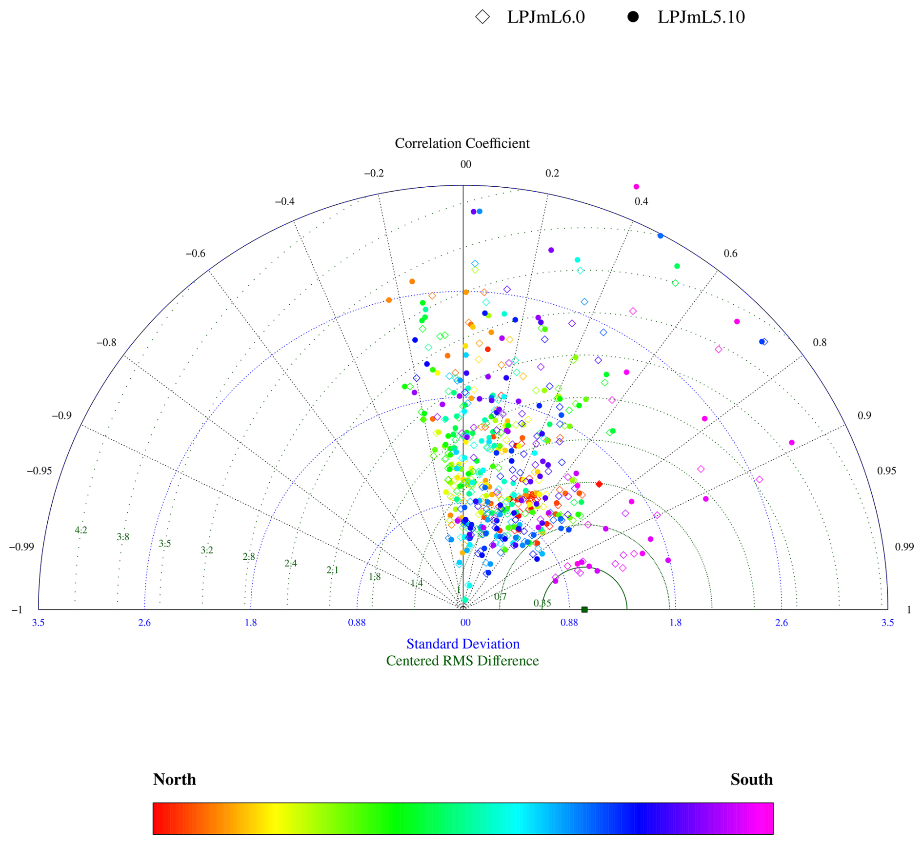
Figure 9 Comparison of simulated discharge with 286 gauges provided by ArcticNET and UNH/GRDC. Stations with basin area > 10 000 km² are taken into account. Gauges are ordered from north to south by color (see legend).

5.5.4 Evapotranspiration fluxes

Simulated ET was compared against eddy-covariance flux tower measurements. While towers provide high-frequency and highly localized ET estimates, the coarse spatial resolution of the simulations introduces a scale mismatch similar to that encountered for NEE.

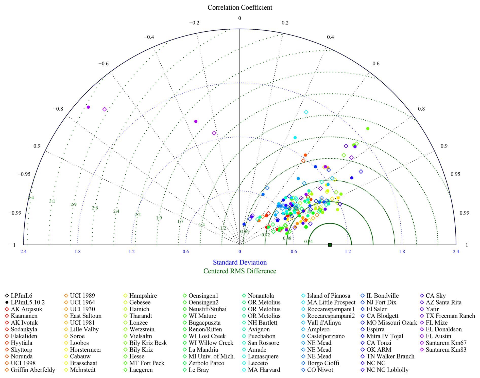
Figure 10 Taylor diagram showing the comparison of simulated evapotranspiration fluxes against eddy-covariance flux tower measurements. Observational data are derived from the FLUXNET network, which provides standardized eddy-covariance measurements of ecosystem–atmosphere carbon and water fluxes (Pastorello et al., 2020).

Model-data agreement of ET is even higher than for NEE, in terms of both correlation coefficients (the model reproduces the temporal variability of ET with greater accuracy) and the CRMSD and the normalized standard deviation (the magnitude of ET fluxes is represented more consistently across sites). This likely reflects the fact that ET is primarily controlled by atmospheric demand and canopy conductance, processes that are more directly constrained by meteorological forcing and vegetation structure in the model, whereas NEE additionally depends on complex carbon turnover processes and ecosystem-specific dynamics.

5.6 Vegetation distribution

A comparison of LPJmL6-simulated actual land cover (natural vegetation plus managed cropland and grassland) witj ESA CCI LC4 land-cover product (Harper et al., 2023) reveals a generally good match in spatial patterns for PFTs (Fig. 11). However, in the temperate and southern boreal zone, ESA CCI LC4 data predominantly show broadleaved summergreen trees, while LPJmL6 simulates a substantially lower abundance of this PFT. Part of this divergence likely stems from the LC-to-PFT reclassification applied to ESA CCI LC4, which can inflate broadleaved summergreen fractions in mosaic and open-forest landscapes and has been shown to introduce spatially structured errors, including overestimation near the taiga–tundra ecotone (Wang et al., 2023b). In the inner tropics, LPJmL6 dominantly simulates broadleaved evergreen trees in line with the observed data, yet it also produces a minor fraction of broadleaved deciduous cover, consistent with the common deciduous–evergreen coexistence in tropical forests (Muehleisen et al., 2024), reflecting the influence of rainfall variability. Mora et al. (2014) suggest that remote sensing data, such as the ESA CCI LC4 dataset, may overestimate the extent of broadleaved evergreen trees in these regions due to challenges in distinguishing between evergreen and deciduous species under dense canopies and during certain seasons. Factors contributing to this misclassification include mixed pixel composition, seasonal variations in leaf phenology, and limitations in sensor resolution. For instance, the complexity of tropical forest structures and the similarity in spectral signatures between different tree species can lead to inaccuracies in classification (Zhong et al., 2024). Finally, while the model effectively simulates the presence of needleleaved deciduous trees in appropriate areas, aligning well with ESA observations, LPJmL6 tends to over-represent their overall abundance in the high-latitude boreal forests of Eurasia and North America.

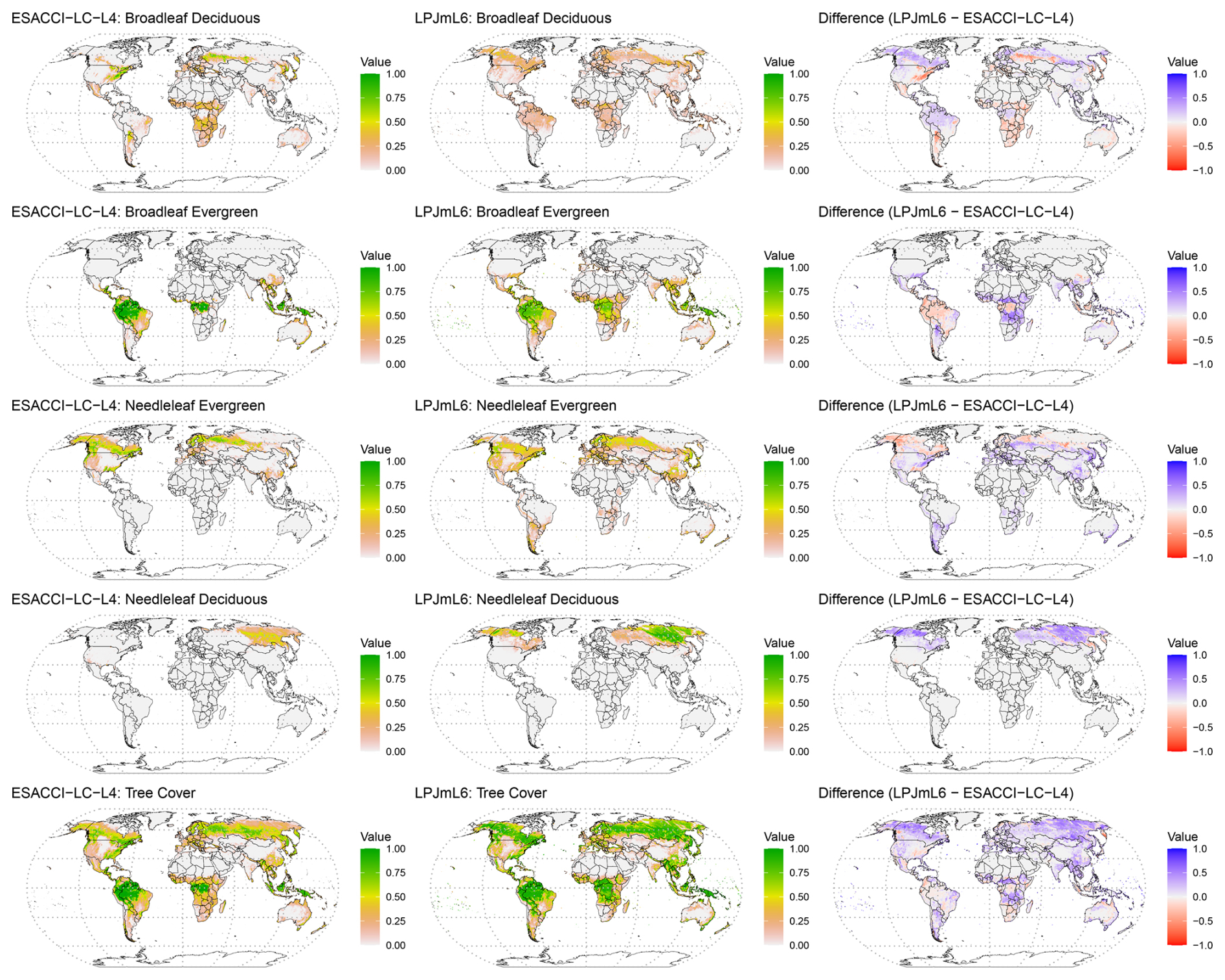
Figure 11 Vegetation distribution of LPJmL6 compared to ESACCI−LC−L4 data (Harper et al., 2023).

Uncertainties also arise from the representation of land use, both in observational products and in the prescribed land-use forcing used to drive LPJmL6. Reconstructions and scenarios of cropland and pasture area differ substantially among datasets, particularly in regions with smallholder or mosaic agriculture, leading to divergent estimates of the area available for natural and managed PFTs (e.g. Prestele et al., 2016; Hurtt et al., 2020; Klein Goldewijk et al., 2017b). These discrepancies propagate into both the LC-to-PFT reclassification of ESA CCI LC4 and the land-use trajectories imposed on LPJmL6, so part of the mismatch between simulated and observed PFT patterns likely reflects uncertainties in land-use data rather than Vegetation dynamics alone.

6 Conclusions

We present LPJmL version 6, including a newly developed process-consistent CH₄ module that links hydrological, vegetation dynamical and biogeochemical processes to atmospheric CH₄ exchange. A new wetland scheme combines a dynamic water table with a CTI-based inundation fraction that is recalculated from the grid-cell CTI distribution, enabling the simulation of spatially and temporally varying anoxic areas within each cell.

Evaluation demonstrates (i) agreement in global wetland area with several inventories, while highlighting a persistent, first-order observational divergence (3.6–11.4 million km²) that translates into different emission potentials; LPJmL6 captures the tropical signal and part of the mid-latitude peak but remains conservative in boreal zones relative to GLWD. (ii) global CH₄ emissions that are consistent with atmospheric measurement constraints when combined with non-modeled sectors that bring the modeled net flux into the 506–630 Tg CH₄ a⁻¹ corridor for 2008–2017. (iii) mechanistic attribution showing diffusion as a leading pathway and ebullition as small, with fires contributing 5 % of natural sources.

LPJmL6 successfully simulates the interactions between environmental factors such as temperature, soil moisture, and vegetation, which govern CH₄ production, oxidation, and transport. Its ability to capture regional and temporal emission trends aligns well with observational datasets and other global estimates, particularly in high-emission regions like tropical wetlands and rice cultivation areas. At the same time, the model highlights remaining uncertainties in CH₄ emissions from agricultural land and high-latitude regions, emphasizing the need for improved constraints on wetland dynamics, managed water fluxes, and small-scale CH₄ sources. Uncertainties are dominated by wetland extent in high latitudes and by agricultural sources, including rice-area dynamics and management, which LPJmL6 now resolves explicitly but for which observational constraints remain limited.

The wetland evaluation should also be interpreted in light of the prescribed CTI representation used by the TOPMODEL formulation. In LPJmL6, CTI does not directly prescribe wetland extent, but provides a fixed sub-grid topographic template that translates the simulated grid-cell mean water-table depth into a saturated fraction. Regional biases in simulated wetland extent may therefore arise either from errors in the simulated water balance and water-table depth, or from limitations of the prescribed CTI distribution and its assumed gamma-shaped sub-grid variability. These limitations are particularly relevant in regions where wetland occurrence is not controlled by local topographic convergence alone. In very flat lowlands, small uncertainties in elevation or slope can strongly affect the inferred CTI distribution, whereas in steep terrain narrow riparian or valley-bottom wetlands may remain unresolved at the model resolution. In floodplains, coastal regions, and managed systems, wetland extent may additionally depend on river inundation, groundwater convergence, backwater effects, drainage, or water management, which are only partly represented by a static CTI-based approach. Consequently, agreement with observed large-scale latitudinal wetland patterns does not imply that the spatial wetland distribution is equally reliable in all regions.

A related uncertainty concerns the agricultural water-input threshold used to represent enhanced drainage on managed land. This threshold is a pragmatic model assumption rather than a parameter derived from site-specific drainage data. It is interpreted as an effective upper limit intended to account for enhanced drainage and water management on agricultural land. Future applications could refine this representation using spatially explicit information on drainage infrastructure, irrigation, and soil hydraulic properties.

Despite these uncertainties, LPJmL6 aligns with bottom-up wetland emission estimates across decades, while recent top-down estimates have converged downward, reducing the historical bottom-up–top-down gap and supporting the process-based approach implemented here. A systematic sensitivity analysis of the newly introduced and modified parameters is an important next step. Such an analysis would help quantify the robustness of the simulated wetland extent, agricultural CH₄ emissions, and total land–atmosphere CH₄ exchange to individual parameter choices and their interactions. Future model development should therefore focus on identifying the most influential parameters and constraining them with independent hydrological, biogeochemical, land-management, and CH₄ flux observations where available.

The implementation of CH₄ dynamics in LPJmL6 represents a significant advancement in the modeling of terrestrial land surface dynamics and, in particular, CH₄ emissions. By integrating CH₄ processes within the broader framework of the global carbon, nitrogen, and water cycles, the model allows for detailed assessments of emissions from different land-use groups, here reported separately for natural wetlands, rice paddies, grasslands, and the remaining cropland. The dynamic representation of wetlands and permafrost processes, combined with hydrological modeling, enhances the understanding of CH₄ flux variability across diverse ecosystems. CH₄ emissions from land use and wetlands are a significant contributor to climate change. Forested wetlands, wetland dynamics, permafrost, and various anthropogenic and natural sources contribute all to the global CH₄ budget. By understanding the complex dynamics of CH₄ emissions and their environmental regulation, effective strategies for mitigating climate change can be developed. Continued research and monitoring of CH₄ emissions are essential for improving our understanding of this potent greenhouse gas and its impact on the planet.

LPJmL6 is a robust tool for understanding the complexities of CH₄ dynamics under current and future climate conditions. These advances allow for more accurate projections of CH₄ emissions, critical for formulating effective climate-mitigation policies. Continued refinement of CH₄-related processes, such as improved parameterization of wetland extents and anthropogenic emission factors, will further increase the realism of LPJmL6-derived surface fluxes. When these fluxes are used in, or coupled to, atmospheric transport and chemistry modules within Earth system modelling frameworks, they can help to better constrain the global CH₄ budget and attribution of observed concentration trends, thereby supporting more robust climate-impact assessments. In addition to enhancing CH₄ representation, the improvements made to the soil water status significantly advance the model's ability to capture land surface dynamics. This enhancement is particularly impactful for simulating water stress in natural vegetation and crops, leading to more accurate representation of plant-water interactions. Notably, this advancement represents a co-benefit of the CH₄-focused implementation, offering improvements beyond CH₄ simulations by strengthening the model’s capacity to simulate hydrological processes and their influence on terrestrial ecosystems.

Appendix A

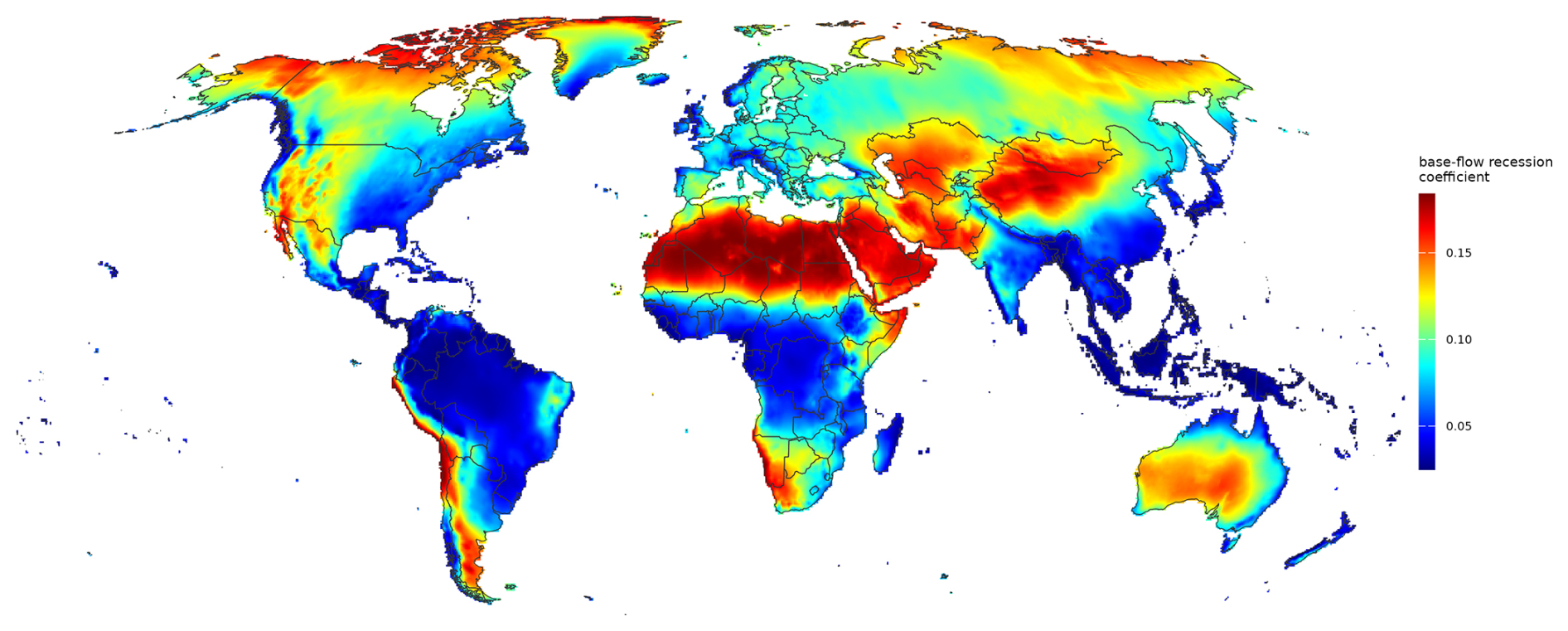
Figure A1 Base-flow recession coefficient determining the outflow rate from groundwater stores as a fraction of the store (Gerten et al., 2018).