BinMod1D v1.0.10: a Python package for explicitly simulating 1D collisional coalescence/breakup processes with corresponding polarimetric radar signatures

This paper details a computationally efficient and versatile Python package (BinMod1D v1.0.10) that explicitly evolves spectral bin distributions and corresponding polarimetric radar variables for rain or snow according to atmospheric collisional coalescence and breakup processes. BinMod1D can be executed as a box model, a 1D steady-state model in height, or a full (time and height) 1D column model utilizing multiple particle categories, each of which can have their own densities, aspect ratios, and fall speeds. Forward simulations of polarimetric radar variables are implemented using standard Rayleigh analytic scattering equations. Two-moment (mass and number) or one-moment (mass only) particle interaction calculations follow a source-based spectral bin method. Bin interaction computations are parallelized using just-in-time (JIT) compilation for high performance. BinMod1D box model solutions are validated using analytic solutions of collision-coalescence using a variety of kernels as well as for breakup and the steady-state balance of coalescence with breakup. BinMod1D capabilities are demonstrated through steady-state simulations of rainfall and snow signatures, as well as vertical profiles of diverse meteorological scenarios. Convergence and timing tests are provided for the meteorological scenario of a cloud to rain transition using a realistic collision kernel and fragment distribution. BinMod1D is intended to enable cloud microphysics and weather radar researchers to efficiently simulate vertical profiles of complex weather events. Such a tool can be used to provide reference solutions for training machine learning models and validating various retrieval methodologies.

1 Introduction

Reference solutions to complex weather phenomena provide a useful way to develop and evaluate new methods for retrieving microphysical variables from weather radar measurements. Such retrievals can involve simple analytic formulas (e.g., Ryzhkov and Zrnić, 2019) or more involved machine learning models (e.g., Chase et al., 2021) that connect radar products like reflectivity to microphysical parameters such as rain or snow rates. Typically, these retrieval equations are developed through a combination of theory and observations, but often without rigorous consideration of microphysical and scattering uncertainties as well as the precise nature of the simulated particle size distribution (PSD). Instead, parameteric approaches, often by assuming an underlying exponential or gamma distribution, are used to connect observed radar variables to desirable microphysical quantities. As a result, however, these parametric approaches sever the important connections between the quantities that are inferred from radar signatures with their underlying microphysical causes.

Of the many microphysical processes in precipitation physics, collision-coalescence and collisional breakup represent two of the most important yet difficult to explicitly simulate. This difficulty can be seen directly from the general equation for collision-coalesence and collsional breakup in time and in height (ignoring horizontal advection terms), which can be expressed as (cf. Mitchell, 1991)

$$\begin{array}{}\text{(1)}& \begin{array}{rl}& {\displaystyle \frac{\partial n(m,z,t)}{\partial t}}+{\displaystyle \frac{\partial \left[v_t\left(m\right)n(m,z,t)\right]}{\mathrm{d}z}}=\\ & {\displaystyle \frac{\mathrm{1}}{\mathrm{2}}}\underset{x=\mathrm{0}}{\overset{m}{\int }}C(m-x,x)n(m-x,z,t)n(x,z,t)\mathrm{d}x\\ & -n(m,z,t)\underset{x=\mathrm{0}}{\overset{\mathrm{\infty }}{\int }}C(m,x)n(x,z,t)\mathrm{d}x+\\ & {\displaystyle \frac{\mathrm{1}}{\mathrm{2}}}\underset{x=\mathrm{0}}{\overset{\mathrm{\infty }}{\int }}\underset{y=\mathrm{0}}{\overset{\mathrm{\infty }}{\int }}B(x,y)P\left(m\right|x,y\left)n\right(x,z,t\left)n\right(y,z,t)\mathrm{d}y\mathrm{d}x-\\ & n(m,z,t)\underset{y=\mathrm{0}}{\overset{\mathrm{\infty }}{\int }}{\displaystyle \frac{B(m,y)n(y,z,t)}{m+y}}\mathrm{d}y\underset{x=\mathrm{0}}{\overset{m+y}{\int }}xP\left(x\right|m,y)\mathrm{d}x,\end{array}\end{array}$$

where $n(m,z,t)$ is the number distribution function for mass m, height z, and time t; v_t(m) is the fall speed for particles of mass m; C(x,y) and B(x,y) are the collision-coalescence and collision-breakup kernels, respectively; and $P\left(m\right|x,y)$ is the conditional fragment distribution that determines the number of mass m fragments generated from collisions involving particles of mass x and y. The left hand side of Eq. (1) represents the tendency and sedimentation terms of the evolving PSD (in terms of mass) whereas the first two right hand side terms represent the gain and loss terms for coalescence and the last two terms represent the gain and loss terms for breakup. Equation (1) reduces to the well-known Smoluchowski equation (Smoluchowski, 1917) when the sedimentation and breakup terms are neglected. The Smoluchowski equation is also frequently referred to by many other names such as the coagulation equation, the stochastic collection equation (Tzivion et al., 1987; Feingold et al., 1988; Bott, 2000; Simmel et al., 2002; Prat and Barros, 2007a), the kinetic collection equation (Alfonso et al., 2008) and the scalar transport equation (McLeod, 1964; Drake, 1972; Drake and Wright, 1972). Equation (1) is difficult to solve for several reasons. First, the integro-differential equation is functional in the coalescence gain term through $C(m-x,x)$ and $n(m-x,z,t)$. As such, standard finite difference numerical methods are not sufficient for directly solving Eq. (1). Secondly, the integral regions are constrained by the particle masses themselves as seen in Eq. (1) with the coalescence gain term and the breakup loss term. This entails that different integration methods are potentially required for different particle m masses. Finally, there are large uncertainties involving the nature and form of the breakup conditional distribution $P\left(m\right|x,y)$. By its nature, $P\left(m\right|x,y)$ should respect detailed mass conservation in the loss term (i.e., $\underset{x=\mathrm{0}}{\overset{m+y}{\int }}xP\left(x\right|m,y)=m+y$), however this condition isn't always exactly met (Feingold et al., 1988). For rain collisional breakup, this has led to several intricate methods that use mixture distributions involving, for example, Gaussian and lognormal distributions to represent the different types of breakup events (i.e., filament, sheet, or disk) as constrained by laboratory measurements (Low and List, 1982a, b; McFarquhar, 2004; Straub et al., 2010).

The complexity of Eq. (1) has historically led to roughly three different types of numerical solution methods: point-based methods, target-based spectral moment methods, and source-based spectral moment methods.

Point-based approaches such as the Berry and Reinhardt (1974) method approximate the number distribution function as a set of discrete points and attempt to solve Eq. (1) by interpolating the functional gain term. This approach is computationally intensive compared to other methods but is considered to be quite accurate and is often used to provide reference solutions for other methods (e.g., Wang et al., 2007). The gain and loss terms are handled separately which leads to mass not being exactly conserved, although with enough points this lack of conservation can be mitigated somewhat.

Target-based spectral moment methods instead evolve bin moments (i.e., number and/or mass) and were originally developed by Bleck (1970) and Enukashvily (1980) and improved upon by Tzivion et al. (1987) and Feingold et al. (1988). In the moment-based approach, Eq. (1) is integrated for each k bin with the kernel x^rdx from the left bin edge x_k to the right bin edge x_k+1. This transforms Eq. (1) into

$$\begin{array}{}\text{(2)}& \begin{array}{rl}& {\displaystyle \frac{\partial M_k^r(z,t)}{\partial t}}+{\displaystyle \frac{\partial S_k^r(z,t)}{\mathrm{d}z}}=\\ & {\displaystyle \frac{\mathrm{1}}{\mathrm{2}}}\underset{m=x_k}{\overset{x_{k+\mathrm{1}}}{\int }}{m}^r\mathrm{d}m\underset{x=\mathrm{0}}{\overset{m}{\int }}C(m-x,x)n(m-x,z,t)n(x,z,t)\mathrm{d}x-\\ & \underset{m=x_k}{\overset{x_{k+\mathrm{1}}}{\int }}{m}^{r}n(m,z,t)\mathrm{d}m\underset{x=\mathrm{0}}{\overset{\mathrm{\infty }}{\int }}C(m,x)n(x,z,t)\mathrm{d}x+\\ & {\displaystyle \frac{\mathrm{1}}{\mathrm{2}}}\underset{m=x_k}{\overset{x_{k+\mathrm{1}}}{\int }}{m}^r\mathrm{d}m\underset{x=\mathrm{0}}{\overset{\mathrm{\infty }}{\int }}\underset{y=\mathrm{0}}{\overset{\mathrm{\infty }}{\int }}B(x,y)P\left(m\right|x,y)\\ & n(x,z,t)n(y,z,t)\mathrm{d}y\mathrm{d}x-\\ & \underset{m=x_k}{\overset{x_{k+\mathrm{1}}}{\int }}{m}^{r}n(m,z,t)\mathrm{d}m\underset{y=\mathrm{0}}{\overset{\mathrm{\infty }}{\int }}{\displaystyle \frac{B(m,y)n(y,z,t)}{m+y}}\mathrm{d}y\\ & \underset{x=\mathrm{0}}{\overset{m+y}{\int }}xP\left(x\right|m,y)\mathrm{d}x,\end{array}\end{array}$$

where $M_k^r(z,t)\equiv \underset{m=x_k}{\overset{x_{k+\mathrm{1}}}{\int }}{m}^{r}n(m,z,t)\mathrm{d}m$ is the rth mass moment of bin k and $S_k^r(z,t)\equiv {\int }_{x_k}^{x_{k+\mathrm{1}}}{m}^r{v}_t\left(m\right)n(m,z,t)\mathrm{d}m$ is the bin's rth mass moment vertical flux. Often, Eq. (2) is used to generate ordinary differential equations for evolving the mass moment (r=1) and the number moment (r=0). While this integral transform increases the dimensionality by one, the advantage is that differential equations for evolving moments of the number distribution function can be represented, at least partially, in terms of the moments themselves. This can be seen schematically in Fig. 1 for collision-coalescence (panel a) and breakup (panel b). In Fig. 1a, each k bin of the target distribution is treated separately one-at-a-time. Each k bin integrates all i and j source bin regions that overlap with the k bin such that $x_k\le x+y\le x_{k+\mathrm{1}}$. This can be seen in Fig. 1a by the red “Gain” region created by the $x+y=x_k$ and $x+y=x_{k+\mathrm{1}}$ diagonal lines. This collision-coalescence gain term for bin k can be numerically calculated by splitting the full integral region (red) into quadrilateral regions of all i and j bin interactions where the individual interacting source i and j bin amounts are shown as black hashes. The loss region for the k bin (blue) is simply a rectangular integration region created by the k (i) bin interaction with each j bin. The gain term is often very lengthy and suffers from the problem of closure, i.e. the subregions are expressed in terms of higher-order moments of the i and j bins. This has led to different closure techniques. For example, Tzivion et al. (1987) uses a nondimensional integral parameter to connect higher order moments to lower order moments whereby the error is small and the maximum possible error can be determined using Schwarz's inequality for a given bin resolution. Because of this error, mass conservation might not be completely satisfied, however the error is apparently minimal. These tricky integral regions are even more complicated when considering collisional breakup as shown in Fig. 1b where these quadrilateral gain and loss regions are represented as three dimensional volumes that are constrained and separated by the $x+y=m$ and $x=y+m$ planes. Other methods such as used by Prat and Barros (2007a) have simplified the lengthy gain and loss integral terms by using the so-called “fixed-pivot” method pioneered by Kovetz and Olund (1969) and later by Kumar and Ramkrishna (1996). In this approach, particles are redistributed by conserving mass and number through a linear interpolation between bin edges and the newly generate particles from the gain terms.

Source-based spectral moment methods are perhaps the most conceptually simple to understand and implement. In these approaches such as detailed in Bott (1998, 2000); Simmel et al. (2002); Wang et al. (2007), each bin-pair interaction (i.e., each pair of i and j bin) and integral region are computed separately and then redistributed to the target distribution bins according to the gain integral regions for each target bin that map to the bin-pair interaction source region. These methods utilize Eulerian geometric mass grids as this ensures that the redistribution will always include a maximum of two bins: a k bin and k+1 bin. By considering each source bin-pair interaction, mass conservation for each bin-pair interaction can be ensured unlike the first two methods. Various source-based models treat the k and k+1 bin partitioning differently. Bott (1998) uses an advection or “flux” scheme whereby the total mass of the i and j collection event are placed in the k bin and a certain fraction of this total mass is then transferred to the k+1 bin by calculating a fractional parameter that is analogous to a weighted Courant number. The Simmel et al. (2002) method is even simpler in that it approximates the collection kernel as a constant such that each source bin-pair interaction provides a fully closed set of ordinary differential equations in terms of the mass and number moments of the interacting distribution bins. A time-dependent linear distribution is then fit between the k and k+1 bins in order to partition the total mass and number between each gain bin.

The source-based method of the Bin Integral Method with Gauss Quadrature (BIMGQ) model by Wang et al. (2007) provided a more rigorous and exact way to perform the k and k+1 bin partitioning compared to the linear flux method of Bott (1998) and the improved version of Bott (2000) as well as the linear discrete method of Simmel et al. (2002). Wang et al. (2007) found that the source bin-pair integral area regions can be calculated exactly through purely geometric considerations and a bilinear approximation of the collection kernel leads to theoretically polynomial terms for each source bin pair. In this way, the gain terms for the k or k+1 bin are expressed in terms of the full source region defined by the i and j bin interaction. Therefore, only the k or k+1 integration calculation is needed as the other bin's calculation can be determined by subtracting the other bin's contribution from the total rectangular source region. In order to simplify these integration calculations, Wang et al. (2007) used a Gaussian quadrature routine which, with enough nodes, would yield the exact polynomial values. Wang et al. (2007) further uses the two predicted moments to diagnose a subgrid linear distribution using the inversion formulas of Enukashvily (1980). Thus, the model evolves both total k bin mass M_k and number N_k whereas Bott (1998) and Bott (2000) evolves the mass distribution function directly by transferring bin-pair interacting masses and then using this mass transfer to fit the new mass distribution function.

While classic Fortran-based collision-coalescence spectral bin solvers exist such as the TAU model (Feingold et al., 1988) and the Bott (1998, 2000) scheme, there has recently been an adoption toward more accessible, modern languages. This transition toward modern accessibility is also reflected in 1D column models and coalescence-based microphysics solvers. For instance, Python-based packages such as LCM1D (Unterstrasser et al., 2020) and PySDM (Bartman et al., 2022) use the Shima et al. (2009) Lagrangian super-droplet method to simulate coalescence. Similarly, Cloudy.jl from Bieli et al. (2022) provides a Julia-based bulk microphysics scheme for simulating cloud microphysics and coalescence. Python-based packages such as the DustPy package from Stammler and Birnstiel (2022) also simulate coagulation but for different disciplines such as astrophysics. For weather radar purposes, it is often not necessary to produce full 3D or 2D simulations when data is often displayed and analyzed in a time/height format such as for quasi-vertical profiles (Ryzhkov et al., 2016), range-defined quasi vertical profiles (Tobin and Kumjian, 2017), columnar vertical profiles (Murphy et al., 2020), Path-columnar vertical profiles (Bukovčić and Krause, 2026). In these cases, it would be convenient for users to specify some initial distribution and then efficiently produce corresponding spectral distributions as well as microphysical and forward simulated radar variables representing mean vertical profiles. Thus, users could use such a simplified model to investigate plausible microphysical explanations for observed vertical radar profiles or for developing retrieval methods from such vertical profiles.

To this end, this paper details a new class-based Python package “BinMod1D” which provides an efficient and versatile spectral bin model along with useful plotting methods. The previous collision-coalescence and breakup methods discussed above often focus on a box model setup and only account for interactions within a single particle class. In contrast, BinMod1D can incorporate as many particle classes as desired as well as custom coalescence and breakup kernels and fragment distributions. Furthermore, the model can be run as a box model, a height-based steady-state model, or a full 1D time/height model. In particular, the steady-state versions of Eqs. (1) and (2) are functionally distinct from the box model and 1D column model in the sense that the tendency term is omitted. Therefore, the ability of BinMod1D to directly simulate steady-state vertical profiles drastically decreases the computational time compared to running the 1D column model to its steady state as done in several rainshaft studies (e.g., Prat and Barros, 2007b; Prat et al., 2012; Kumjian and Prat, 2014). The BinMod1D model is based upon the source-based approach of Wang et al. (2007) but with several computational optimizations. For example, the model heavily utilizes Numba (Lam et al., 2015) which automatically parallelizes calculations for computationally intensive model runs. The model can also be run using the 2-moment (mass and number) subgrid linear distribution approach of Wang et al. (2007) or as a 1-moment (mass only) subgrid uniform distribution approach. The BinMod1D methodology is described in more detail in Sect. 2 along with the Python class architecture. Section 3 provides several box model, steady-state, and column model results derived from Jupyter notebook examples available in the BinMod1D v1.0.10 repository (Dunnavan, 2026a). Section 4 performs a computation speed and accuracy test using a realistic meteorological scenario for both two-moment and one-moment calculations. Finally, Sect. 5 discusses several potential uses of BinMod1D and likely future additions and improvements to the package.

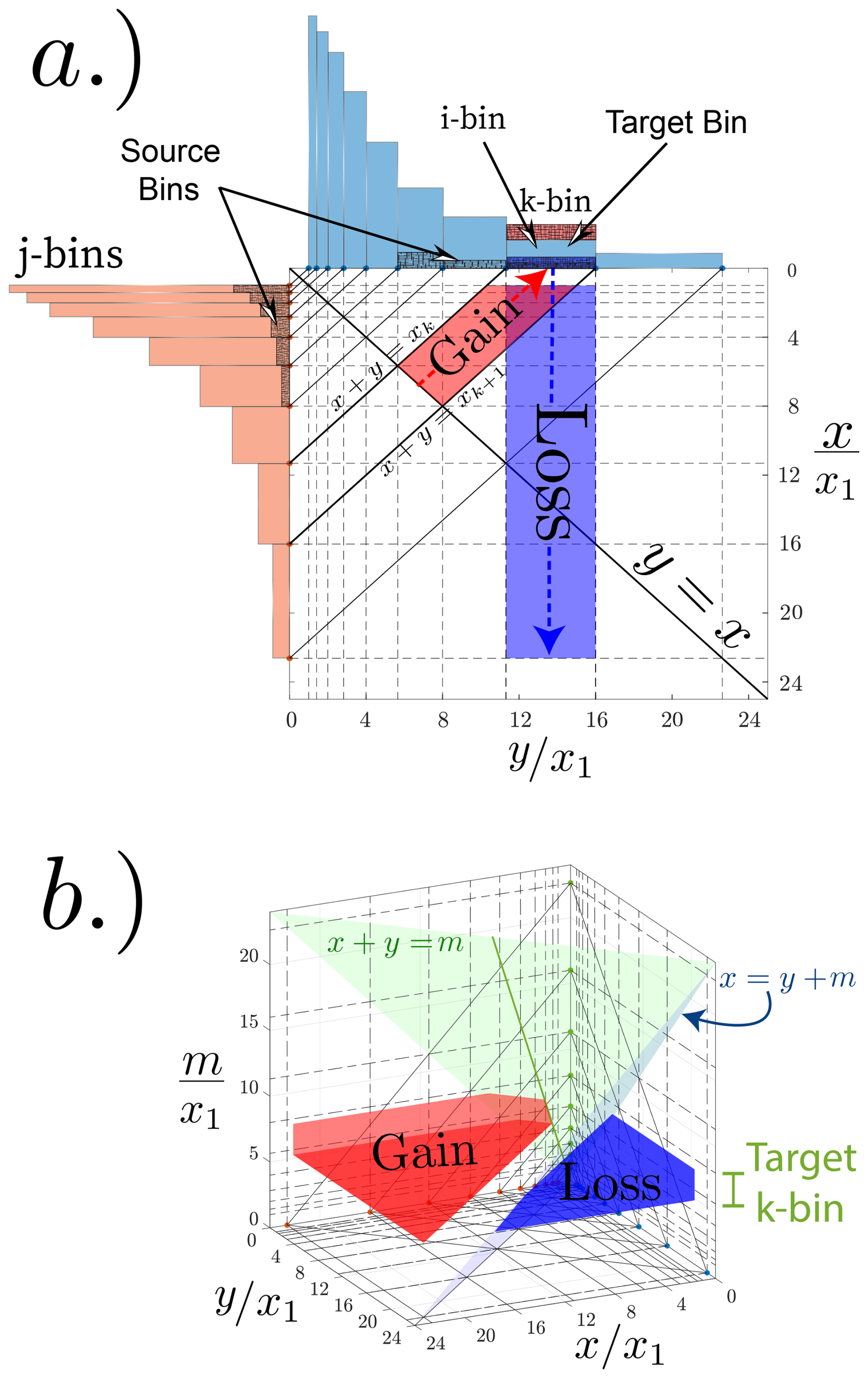
Figure 1 The spectral bin “method-of-moments” target-based integration regions from Feingold et al. (1988) for: (a) collision-coalescence and (b) collisional breakup where s_bin=2.

2 Methodology

2.1 Numerical integration method

For a single distribution with bin k, the moment equations (Eq. 2) can be cast in the following discrete form for moment order r:

$$\begin{array}{}\text{(3)}& \begin{array}{rl}& {\displaystyle \frac{\partial M_k^r(z,t)}{\partial t}}+{\displaystyle \frac{\partial \left[S_k^r(z,t)\right]}{\mathrm{d}z}}\approx {\displaystyle \frac{\partial M_k^r(z,t)}{\partial t}}+v_{t,k}{\displaystyle \frac{\partial M_k^r(z,t)}{\mathrm{d}z}}\\ & =\sum _{i+j\to k}{\widehat{C}}_{\mathrm{gain},k}^r(i,j,z,t)+\sum _{max(i,j)\ge k\to k}{\widehat{B}}_{\mathrm{gain},k}^r(i,j,z,t)\\ & -\sum _{i=k,j|i,j=k}{\widehat{D}}_{\mathrm{loss},k}^r(i,j,z,t)=I_k^r(z,t),\end{array}\end{array}$$

where ${\widehat{D}}_{\mathrm{loss},k}^r(i,j,z,t)\equiv {\widehat{C}}_{\mathrm{loss},k}^r(i,j,z,t)+{\widehat{B}}_{\mathrm{loss},k}^r(i,j,z,t)$ are the combined bin moment losses from the i−j bin-pair interaction¹, and the sedimentation shown as the second term on the left hand side of Eq. (3) is approximated using the bin mass midpoint fall speed value in order to achieve moment closure when solving the stochastic collection/breakup equation. The terms $C_{\mathrm{gain},k}^r(i,j,z,t)$ and $B_{\mathrm{gain},k}^r(i,j,z,t)$ are the gain terms for each k bin moment $M_k^r$ due to coalescence and breakup, respectively for i−j bin-pair. Each term on the right hand side represents a separate integral

$$\begin{array}{}\text{(4a)}& {\displaystyle }\begin{array}{rl}& {\widehat{C}}_{\mathrm{gain},k}^r(i,j,z,t)=\\ & \underset{{\mathrm{\Omega }}_k}{\int }{x}^{r}C(x,y|i,j\left)n_{x|i,j,z,t}\right(x\left)n_{y|i,j,z,t}\right(y)\mathrm{d}{\mathrm{\Omega }}_k\end{array}\text{(4b)}& {\displaystyle }\begin{array}{rl}& {\widehat{B}}_{\mathrm{gain},k}^r(i,j,z,t)=\underset{m=k}{\overset{k+\mathrm{1}}{\int }}{m}^r\underset{x=x_i}{\overset{x_{i+\mathrm{1}}}{\int }}\underset{y=y_i}{\overset{y_{i+\mathrm{1}}}{\int }}B(x,y|i,j\left)P\right(m|i,j)\\ & n_{x|i,j,z,t}\left(x\right)n_{y|i,j,z,t}\left(y\right)\mathrm{d}m\mathrm{d}x\mathrm{d}y\end{array}\text{(4c)}& {\displaystyle }\begin{array}{rl}& {\widehat{D}}_{\mathrm{loss},k}^r(i,j,z,t)=\underset{x=x_i}{\overset{x_{i+\mathrm{1}}}{\int }}\underset{y=y_i}{\overset{y_{i+\mathrm{1}}}{\int }}{x}^r\left[C(x,y|i,j)+B(x,y|i,j)\right]\\ & n_{x|i,j,z,t}\left(x\right)n_{y|i,j,z,t}\left(y\right)\mathrm{d}x\mathrm{d}y\end{array}\end{array}$$

where

$$\begin{array}{}\text{(5a)}& {\displaystyle }C(x,y|i,j)\equiv E_{\mathrm{col}}{E}_{\mathrm{s}}K(x,y|i,j)\text{(5b)}& {\displaystyle }B(x,y|i,j)\equiv E_{\mathrm{col}}(\mathrm{1}-E_{\mathrm{s}}\left)E_{\mathrm{b}}K\right(x,y|i,j),\end{array}$$

and $K(x,y|i,j)$ is the collection kernel which dictates the physics of the x and y interactions in the $x_i\le x\le x_{i+\mathrm{1}}$ and $y_i\le y\le y_{i+\mathrm{1}}$ rectangular space for the i−j bin-pair. Ω_k represents the region of the i−j bin-pair (x,y) space that leads to a gain in bin k.

The awkward summation notation in Eq. (3) indicates the conditions under which i−j bin-pair interactions leads to a gain or loss in the k bin. For the first term (coalescence), this means summing all i−j pairs where $x+y=m$ such that $x_k\le m\le x_{k+\mathrm{1}}$. For the second term (breakup) this means summing all i−j pairs where $k\le max(i,j)$ such that the bin-pair interaction leads to a gain in the k bin. For the third term (combined total loss), this means summing all i−j pairs that involve bin k. Note that cases of self-collection (i.e., collection of bins from the same distribution) necessarily requires the calculation of only one of these pairs. $I_k^r(z,t)$ therefore represents the full interaction of all i−j bin pairs that lead to moment changes in the k bin. Therefore, BinMod1D solves one of the three following equations depending upon the user's chosen mode

$$\begin{array}{}\text{(6a)}& {\displaystyle \frac{\mathrm{d}{M}_k^r\left(t\right)}{\mathrm{d}t}}=I_k^r\left(t\right)\text{(Box Model)}\text{(6b)}& {\displaystyle }{v}_{t,k}{\displaystyle \frac{\mathrm{d}{M}_k^r\left(z\right)}{\mathrm{d}z}}=I_k^r\left(z\right)\text{(Steady-state Model)}\text{(6c)}& {\displaystyle }\begin{array}{rl}& {\displaystyle \frac{\partial M_k^r(z,t)}{\partial t}}+v_{t,k}{\displaystyle \frac{\partial M_k^r(z,t)}{\partial z}}=I_k^r(z,t)\\ & \text{(Full 1D Column Model)},\end{array}\end{array}$$

for either r=1 (mass; 1 moment) or r=1 and r=0 (mass and number; 2 moments). These equations for $M_k^{\mathrm{1}}(z,t)\equiv M_k(z,t)$ (1 moment) or M_k(z,t) and $M_k^{\mathrm{0}}(z,t)\equiv N_{t,k}(z,t)$ (2 moment) are numerically solved using an upwind advection scheme in height and a generalized Runge-Kutta method (with options of 1st to 4th order) in time. Adaptive time steps are also employed to ensure numerical stability where the target timstep is determined from either the dt parameter or, for the steady-state mode, the calculated residence time for each bin while solving $I_k^r(z,t)$. Generally these split time steps are not necessary and are not even used. However, these additional steps become necessary in regimes with, for example, large numbers of particle interactions with aggressive breakup.

The main computational load and complexity of the BinMod1D package comes from using the Wang et al. (2007) approach to solve $I_k^r$ for r=1 (mass; one-moment prediction) or r=1 and r=2 (mass and number; two-moment prediction). Figure 2 shows a schematic of the Wang et al. (2007) approach using example interactions for self-collection (j−j) and cross-collection (i−j). For this schematic, it is assumed that a distribution with i bins is interacting with a distribution of j bins to produce particles that will be added to a distribution with k bins. Each time/height step therefore calculates each combination of i and j bin-pair interactions and transfers particles (i.e., total mass or total mass and number) from the i and j bin to the k and k+1 bins of a target distribution. Here, distribution k and j are assumed identical although the procedure works if k and j are different. As in Wang et al. (2007) and other coagulation solvers, BinMod1D uses a geometric mass grid where bin edges are determined by

$$\begin{array}{}\text{(7)}& x_i\equiv x_{\mathrm{1}}{\mathrm{2}}^{(i-\mathrm{1})/s_{\mathrm{bin}}}\end{array}$$

for $i=\mathrm{1},\mathrm{2},\mathrm{3},\mathrm{\dots },N_{\mathrm{bin}}+\mathrm{1}$ (see Eq. 9 from Wang et al., 2007) and s_bin in Eq. (7) is an integer resolution parameter which governs the number of bins per mass doubling. With the Eq. (7) mass grid, self-collection of an i=j and j bin results in a gain to the $k=j+s_{\mathrm{bin}}$ bin (green lines in Fig. 2a). This can be seen by $x_j+x_j=\mathrm{2}{x}_j\to x_{j+s_{\mathrm{bin}}}$ and $x_{j+\mathrm{1}}+x_{j+\mathrm{1}}=\mathrm{2}{x}_{j+\mathrm{1}}\to x_{j+s_{\mathrm{bin}}+\mathrm{1}}$ mappings (skewed green arrows). The gain integrals for cross-collection, in general, will cover two bins: k and k+1. An example of cross-collection is shown by the rectangular red/purple region in Fig. 2a. Here the $x+y=x_{k+\mathrm{1}}$ line which delineates the k and k+1 bins cuts directly through the rectangular source region defined by the i and j bin interaction. As a result, the quadrilateral region that is above this line maps to the k (red) bin whereas the quadrilateral region below this line maps to the k+1 (purple) bin. As shown by Fig. 2b, these quadrilateral regions can be segmented into rectangular and triangular parts, each of which can be integrated separately. As stated in Sect. 1, only one of these quadrilateral regions needs to be calculated as the other one can be determined through continuity with the full rectangular region integration needed for computing the loss term for the i and j bin interaction. While the projected integration region for the mass and number gain integrals cuts through both the k and k+1 bins, the values will be added to each respective bin in its entirely. This is shown schematically in Fig. 2 as “smearing” the total added amounts from the left bin edge to the right edge (shown here as red and purple colored transparencies). Each integration region type is therefore treated separately and the general solution is to treat each k or k+1 bin sub region as either a triangle, rectangle, or a triangle and a rectangle as in Fig. 2b. As in Wang et al. (2007), moment closure is ensured by performing a bilinear interpolation of the collision/coalescence kernel in the form: $K(x,y)\equiv a+bx+cy+dxy$, for each source bin-pair interaction. Notice that this form is slightly different than Eq. (22) in Wang et al. (2007) in order to elucidate the polynomial form of the bilinear collection kernel approximate in the integrand of each integral:

$$\begin{array}{}\text{(8)}& \begin{array}{rl}& K(x,y)n_x\left(x\right)n_y\left(y\right)\approx K_{\mathrm{00}}+K_{\mathrm{10}}x+K_{\mathrm{01}}y+K_{\mathrm{11}}xy\\ & +K_{\mathrm{20}}{x}^{\mathrm{2}}+K_{\mathrm{21}}{x}^{\mathrm{2}}y+K_{\mathrm{02}}{y}^{\mathrm{2}}+K_{\mathrm{12}}x{y}^{\mathrm{2}}+K_{\mathrm{22}}{x}^{\mathrm{2}}{y}^{\mathrm{2}}.\end{array}\end{array}$$

As can be seen from Eqs. (4) and (5), all integrals use the same collection kernel $K(x,y|i,j)$ where BinMod1D v1.0.10 considers only a single type of kernel (e.g., hydrodynamic) between each combination of distribution categories. Therefore, the four types of integrals that need to be solved for each term are

$$\begin{array}{}\text{(9a)}& {\displaystyle }\underset{{\mathrm{\Omega }}_{\mathrm{R}}}{\int }K(x,y)n_x\left(x\right)n_y\left(y\right)\mathrm{d}{\mathrm{\Omega }}_{\mathrm{R}}\left(\text{number loss/gain}\right)\text{(9b)}& {\displaystyle }\underset{{\mathrm{\Omega }}_{\mathrm{R}}}{\int }xK(x,y)n_x\left(x\right)n_y\left(y\right)\mathrm{d}{\mathrm{\Omega }}_{\mathrm{R}}\left(x\text{ mass loss}\right)\text{(9c)}& {\displaystyle }\underset{{\mathrm{\Omega }}_{\mathrm{R}}}{\int }yK(x,y)n_x\left(x\right)n_y\left(y\right)\mathrm{d}{\mathrm{\Omega }}_{\mathrm{R}}\left(y\text{ mass loss}\right)\text{(9d)}& {\displaystyle }\underset{{\mathrm{\Omega }}_{\mathrm{R}}}{\int }(x+y)K(x,y)n_x\left(x\right)n_y\left(y\right)\mathrm{d}{\mathrm{\Omega }}_{\mathrm{R}}(x+y\text{ mass gain}),\end{array}$$

where Ω_R is either a rectangular region, a triangular region, or a polygonal region that can be split into a triangular and a rectangular region. Rectangular regions can simply be integrated directly into polynomials of one degree higher than in the integrand. However, the number of polynomials from analytical integration of the triangular regions increases geometrically with higher order integrand polynomials. For these triangular regions, the number of monomials for the mass gain integrals becomes very high. To simplify the calculations, the Wang et al. (2007) quadrature idea is used to calculate these triangular region integrals using the 7-point Dunavant rule (Dunavant, 1985) to determine weights and locations for the quadrature rule. The 7-point rule is used here specifically because this rule produces exact values for triangular region integrations with polynomial integrands up to order 5 which is the maximum possible order for subgrid linear distributions of BinMod1D 2-moment scheme.

The Wang et al. (2007) method described above pertains to coalescence only. However, the same general source-based method can be extended to include collisional breakup as well. This new method for collisional breakup is shown schematically in Fig. 3 for an example i and j bin-pair interaction. The BinMod1D model first calculates the total breakup mass (1 moment) or mass and number (2 moments) for the i−j interaction using Eq. (4c). Then, the conditional fragment distribution $P\left(m\right|x,y)$ is determined by taking the assumed fragment distribution form P_f(m) and scaling this distribution by ensuring mass continuity with the total mass integral from the full rectangular i−j region (i.e., $P_{\mathrm{f},i-j}=P_{\mathrm{f}}/\mathrm{\Delta }{M}_{\mathrm{b},i-j}$). Then, the total mass (or mass and number) are binned by integrating each k bin from k=0 to $k=max(i,j)$². This is shown schematically as partitioning the full rectangular integration region into k rectangular subregions, each of which represents the integrated amounts added to each k bin for the j−i bin interaction. Users can specify various fragment distributions by either using examples from the habits.py module or by specifying the fragment dictionaries themselves. These integrations are computed beforehand for a fixed fragment distribution form.

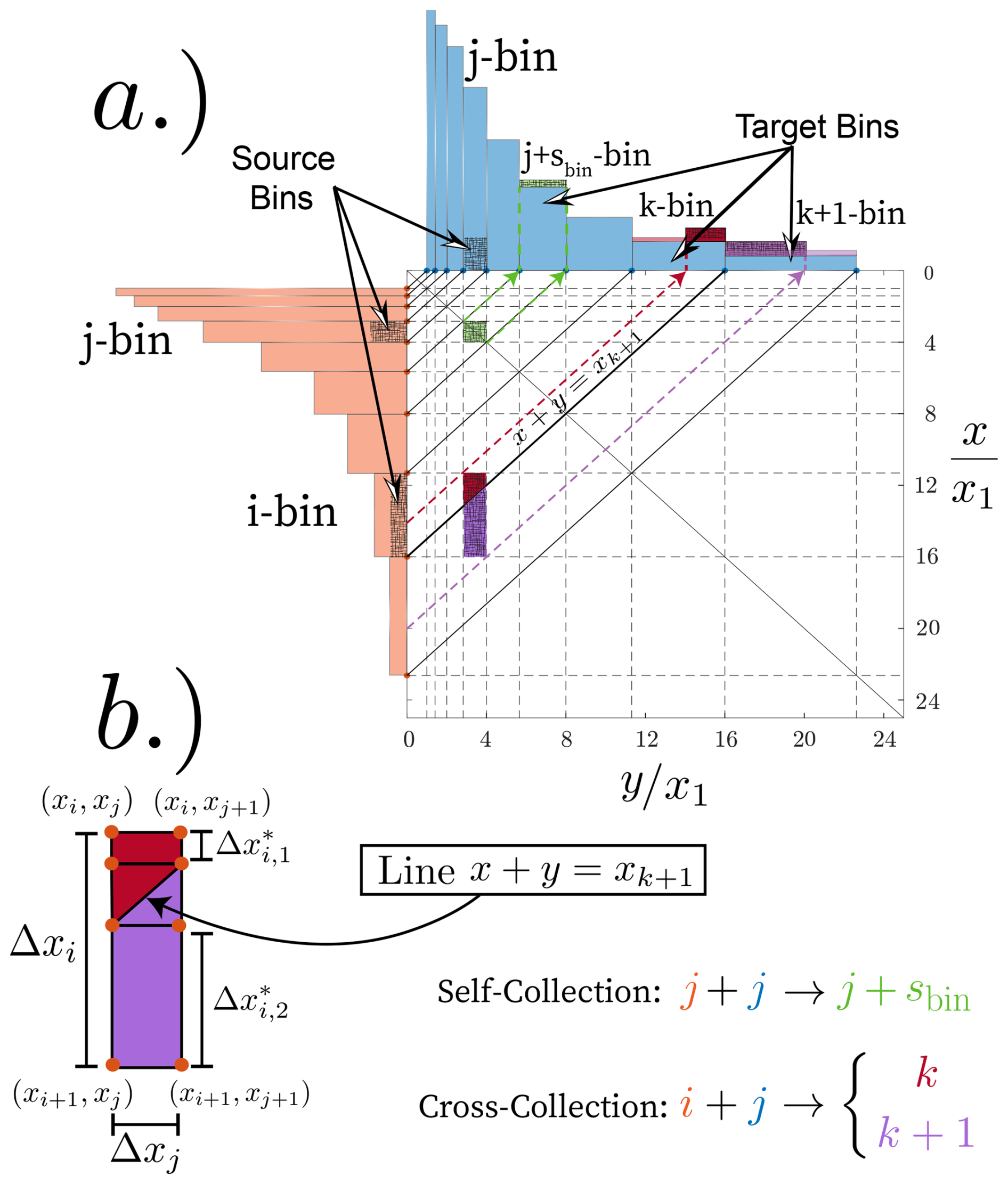
Figure 2 The source-based spectral bin model of Wang et al. (2007) (cf. their Fig. 2) using s_bin=2 resolution. (a) Shows an example of the self-collection square integration region and target mapping (j+j; green), whereas the rectangular region (b) illustrates cross-collection (i+j). The geometry in (b) illustrates how the integration is handled exactly by splitting the integrals into rectangles and triangles that are used to segregate the target amounts in k and k+1 bins (see Fig. 4 from Wang et al., 2007).

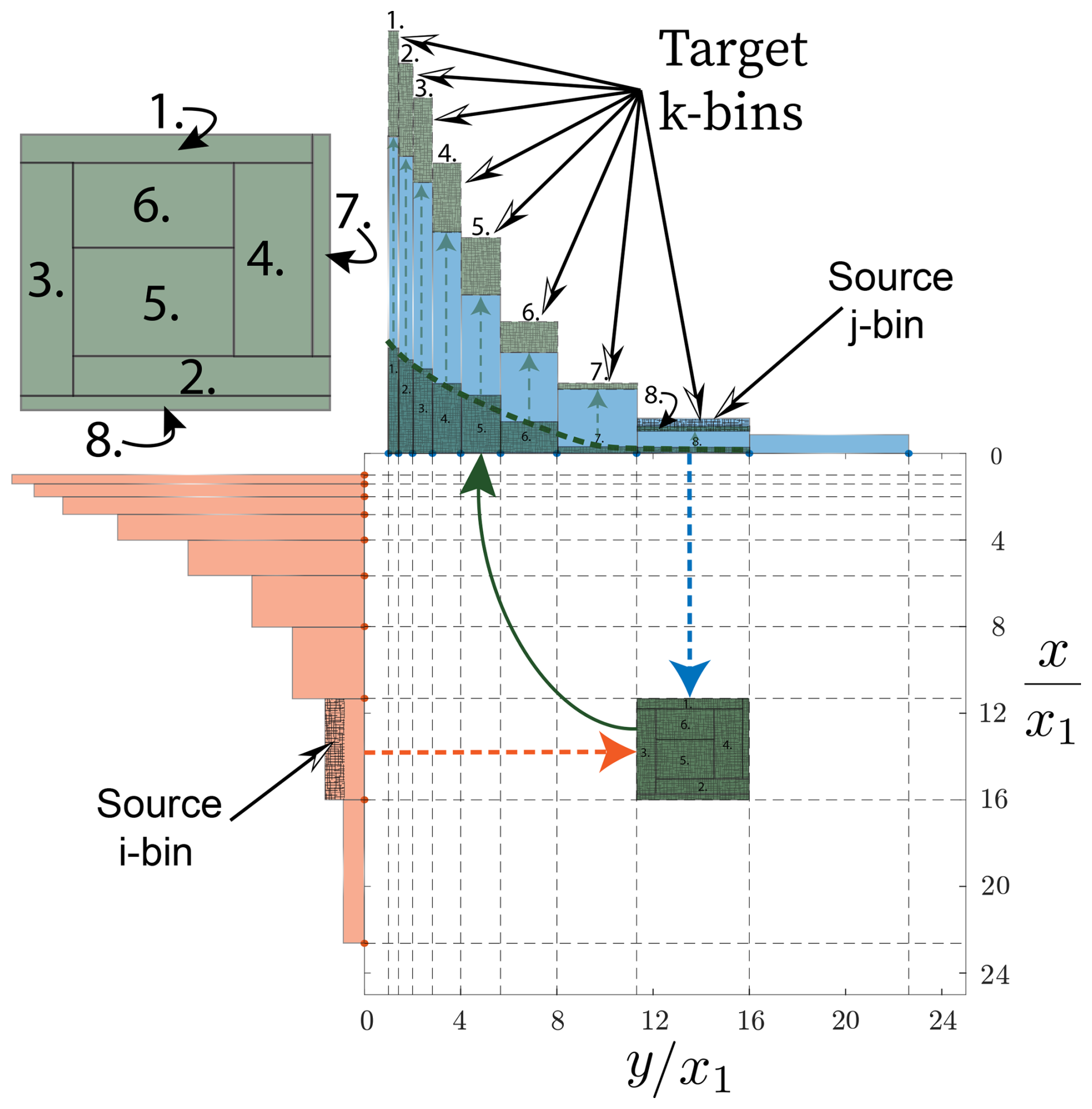
Figure 3 The collisional breakup methodology of BinMod1D. Each collision event between i and j bins represents a rectangular integration space from which the total mass is determined. The total mass is binned following the $P\left(m\right|x,y)$ conditional distribution (dashed green line) and then rescaled by ensuring mass continuity of the entire rectangular integral region. Schematically, this can be thought of as breaking the source bin-pair interaction integration region into k pieces (see inset) which are then normalized by the total mass, binned, and added to the k distribution (here shown to be identical to the j distribution).

BinMod1D diagnoses each distribution's linear subgrid distribution set of parameters after each time/height step when N_k and/or M_k evolves. This form is given as

$$\begin{array}{}\text{(10a)}& {\displaystyle }n\left(x\right)=a_{k}x+c_k,\text{2-moment}\text{(10b)}& {\displaystyle }n\left(x\right)=c_k\text{1-moment.}\end{array}$$

where the Eq. (10a) formulas for a_k and c_k can be derived from equations 15 through 20 in Wang et al. (2007). Each bin therefore has four separate parameters that govern the subgrid linear distribution function: a_k, c_k, x_k,1, and x_k,2. Note that when moments=1, a subgrid uniform distribution across each bin is used such that these parameters are diagnosed as: $x_{k,\mathrm{1}}=x_k$, $x_{k,\mathrm{2}}=x_{k+\mathrm{1}}$, a_k=0, and $c_k=\mathrm{2}{M}_k/(x_{k+\mathrm{1}}^{\mathrm{2}}-x_k^{\mathrm{2}})$ and $N_k=M_k/{\stackrel{\mathrm{‾}}{x}}_k$, where ${\stackrel{\mathrm{‾}}{x}}_k$ is the bin midpoint mass.

To simplify the calculations, each $I_k^r$ term is computed separately and then recombined for each k bin for each distribution. This is because each i−j interaction will generate gains in multiple, scattered bins. To perform these calculations, BinMod1D first flattens all arrays needed for each bin-pair interaction such that each bin-pair interaction has a unique set of integration values and destination bin indices. Then, BinMod1D efficiently utilizes “just-in-time” (JIT) compilation using the Numba Python package to perform the interaction integration calculations in parallel for all bin-pair interactions at all heights at once. This leads to BinMod1D effectively using machine code to loop through each possible bin-pair interaction even when utilizing multiple distributions in the full 1D column model mode for all heights at once. For coalescence, the loss and gain transfer calculations are performed for each bin-pair interaction first using Numba-compiled loops and are stored in arrays with the length of the total number of bin pairs. The transfer of the calculation from the i−j source space to the k and k+1 target space (Fig. 2) is performed through scattered addition using the Numpy add.at method after all integration calculations are performed and stored. Collisional breakup, on the other hand, uses additional Numba-compiled loops after the breakup gain amounts are calculated to transfer the breakup fraction of the total i−j bin-pair source loss to each k target bin (see Fig. 3) in the breakup distribution. Multidimensional temporary arrays are used to prevent race conditions during this transfer process where the Numba thread number, heights, and bins represent a three dimensional buffer array from which the transfer sequentially adds to each bin and height in the fragment distribution index for M_k (and N_k if 2 moments are used). Several core BinMod1D components, including the parallelizable interaction kernel computations, were algorithmically streamlined using Google Gemini Pro as a code-refinement tool to ensure maximum computational speed in standard Python environments.

2.2 BinMod1D class architecture and workflow

Comprehensive documentation and step-by-step tutorials that cover BinMod1D model initialization, parameter specification, customization, and more are provided in the software documentation (Dunnavan, 2026b). This section provides only a technical overview of the BinMod1D methodology and classes.

Regardless of how the model is run, the general workflow is the same. Users first initialize a spectral_1d object with a set of input parameters that govern the initial distribution, habit parameters, processes included, and model mode. Each spectral_1d object represents a separate model instance of BinMod1D where the object performs several tasks:

1. It uses the user's prescribed number of distributions and other input parameters and initializes an object of the Interaction class which is used to determine the bin-pair interactions when the run method is called. If moments=1 is specified, then bin-pair interactions for collision-coalescence is precalculated whereas moments=2 bin interaction calculations are computed during model runtime.

2. It runs the BinMod1D model with the run method which runs the model as a box model, a steady-state model, or a full 1D (time/height) model with either one or two predicted moments for each bin. The run mode selection depends upon the prescribed inputs for parameters t_max, z_bot and z_top. If $t_{max}>\mathrm{0}$ and z_bot=z_top then the box model is run, if $t_{max}=\mathrm{0}$ and z_bot<z_top then the steady-state model is run, and if $t_{max}>\mathrm{0}$ and z_bot<z_top then the full 1D model is run.

3. It stores each distribution's M_k or (M_k and N_k) value in a 4D array where the array is indexed by distribution, height, bins, and output time.

4. It plots the model results using methods that start with plot_ (e.g., spectral_1d.plot_dists()).

5. It writes model output after the run method is called to a netcdf file with the write_netcdf method.

Users can initialize the particle size distribution(s) using one of six different methods using the spectral_1d input init_method:

1. init_method = 'gamma': The initial distribution is a gamma distribution with parameters specified by the user as additional arguments in spectral_1d.

2. init_method = 'analytical':

   The initial distribution is defined using a custom Python lambda function.

3. init_method = 'empirical':

   The initial distribution is prescribed using edges and number distribution function value evaluated at the prescribed bin midpoints.

4. init_method = 'empirical_counts':

   As in init_method = 'empirical' but where users prescribe bin counts rather than number distribution function values.

5. init_method = 'direct':

   The user directly prescribes the bin masses (M_bins) and/or bin numbers (N_bins) along with bin edges.

6. empty:

   The initial distribution is initialized with no bin mass or number amounts.

When spectral_1d is first initialized, an initial distribution using the dist class is binned according to the user's input parameter specifications. If users use the input init_method = 'gamma' (default), then the initial binned distribution is calculated from a gamma distribution of the form

$$\begin{array}{}\text{(11)}& \begin{array}{rl}{n}_{\mathrm{0}}\left(D\right)& =\mathrm{1000}{\displaystyle \frac{N_{t,\mathrm{0}}}{\mathrm{\Gamma }({\mathit{\mu }}_{\mathrm{0}}+\mathrm{1})}}({\mathit{\mu }}_{\mathrm{0}}+\mathrm{4}{)}^{{\mathit{\mu }}_{\mathrm{0}}+\mathrm{1}}{\displaystyle \frac{\mathrm{1}}{D_{m,\mathrm{0}}}}{\left({\displaystyle \frac{D}{D_{m,\mathrm{0}}}}\right)}^{{\mathit{\mu }}_{\mathrm{0}}}\\ & \exp \left[-({\mathit{\mu }}_{\mathrm{0}}+\mathrm{4}){\displaystyle \frac{D}{D_{m,\mathrm{0}}}}\right]\end{array}\end{array}$$

where n₀(D) has units of m⁻³ mm⁻¹ with a full initial number concentration N_t,0 in L⁻¹, full mean volume diameter D_m in mm, and shape parameter μ. Note the prescribed N_t,0 and D_m,0 values represent values that are valid for the full distribution from (0,∞) whereas the total binned values for N_t and D_m will depend upon the bin resolution s_bin and the minimum and maximum bin masses (sizes). Users who instead prefer the gamma distribution form

$$\begin{array}{}\text{(12)}& n_{\mathrm{0}}\left(D\right)=N_{\mathrm{0}}{D}^{{\mathit{\mu }}_{\mathrm{0}}}\exp (-{\mathrm{\Lambda }}_{\mathrm{0}}D)\end{array}$$

can diagnose the spectral_1d parameters with the equations

$$\begin{array}{}\text{(13a)}& {\displaystyle }{\mathit{\mu }}_{\mathrm{0}}={\mathit{\mu }}_{\mathrm{0}}\text{(13b)}& {\displaystyle }{D}_{m,\mathrm{0}}={\displaystyle \frac{{\mathit{\mu }}_{\mathrm{0}}+\mathrm{4}}{{\mathrm{\Lambda }}_{\mathrm{0}}}}\text{(13c)}& {\displaystyle }{N}_{t,\mathrm{0}}=N_{\mathrm{0}}{\displaystyle \frac{\mathrm{\Gamma }({\mathit{\mu }}_{\mathrm{0}}+\mathrm{1})}{{\mathrm{\Lambda }}^{{\mathit{\mu }}_{\mathrm{0}}+\mathrm{1}}}},\end{array}$$

where Λ₀ has units of mm⁻¹ and N₀ has units of $\mathrm{m}{}^{-\mathrm{3}}{\mathrm{mm}}^{-({\mathit{\mu }}_{\mathrm{0}}+\mathrm{1})}$. The gam_norm parameter determines if instead the initial gamma distribution is normalized to have a total mass concentration of unity. Thus, when gam_norm=True the form of the initial gamma distribution is instead with respect to mass m and normalized as

$$\begin{array}{}\text{(14)}& {\stackrel{\mathrm{̃}}{n}}_{\mathrm{0}}\left(m\right)={\displaystyle \frac{N_{t,\mathrm{0}}}{\mathrm{\Gamma }\left({\mathit{\nu }}_{\mathrm{0}}\right)}}{\displaystyle \frac{\mathrm{1}}{\stackrel{\mathrm{‾}}{m}}}{\mathit{\nu }}_{\mathrm{0}}^{{\mathit{\nu }}_{\mathrm{0}}}{\left({\displaystyle \frac{m}{\stackrel{\mathrm{‾}}{m}}}\right)}^{{\mathit{\nu }}_{\mathrm{0}}-\mathrm{1}}\exp \left[-{\mathit{\nu }}_{\mathrm{0}}{\displaystyle \frac{m}{\stackrel{\mathrm{‾}}{m}}}\right],\end{array}$$

where ${\mathit{\nu }}_{\mathrm{0}}={\mathit{\mu }}_{\mathrm{0}}+\mathrm{1}$. Equation (11) is generally used in practice but Eq. (14) is often used when comparing numerical results to known analytical solutions of the stochastic collection equation (see Sect. 3.1 and the BM1D_analytical_examples.ipynb Jupyter notebook for example). When Eq. (14) is used for gam_norm=True, users will specify the N_t,0, M_t,0, μ₀, and x₀ parameters with dist_var="mass" (where $\stackrel{\mathrm{‾}}{m}\equiv M_{t,\mathrm{0}}/N_{t,\mathrm{0}}$) whereas when Eq. (11) is used for gam_norm=False users will specify N_t,0, D_m,0, μ₀, D₁ parameters along with dist_var="size". Alternatively, users can directly specify $\stackrel{\mathrm{‾}}{m}$ with the mbar0 input parameter. The D₁ (x₀) parameter determines the minimum left hand bin edge size (mass) used for the first bin when specifying dist_var="size" (dist_var="mass").

Users can specify the number and type of distributions used in spectral_1d by adding subsequent distributions to the list in the habit_params input parameter (e.g., habit_params=["snow","fragments"]). The length of habit_params determines the number of separate distributions that are solved where the names refer to the particle microphysical parameters in habits.py that are used for each distribution. The spectral_1d input parameter kernel determines the type of interaction kernel (i.e., K(x,y)) with the kernel input (e.g., kernel="Hydro", for the hydrodynamic or gravitational kernel). Users can explicitly set the cc_dest and br_dest input parameters when more than one distribution is specified. Here, cc_dest and br_dest determine the distribution (i.e., category) destination of coalesced and breakup bin-pair interactions, respectively where integer values are given from 1 to len(habit_params). For example, a two-category BinMod1D simulation where the first distribution represents a primary category such as ice crystals and the second category represents snow aggregates can be initialized with cc_dest=2 and habit_params=["snow","snow"]. Similarly, a two-category BinMod1D simulation with snow (and its aggregates) as one category and breakup fragments as the second category can be specified with cc_dest=1, br_dest=2, and habit_params=["snow","fragments"]. Only one distribution/category is used when cc_dest= br_dest=1 (the default behavior). Collision (E_col), coalescence (E_s) and breakup (E_b) efficiencies are treated as constants that can be passed into spectral_1d directly (e.g., spectral_1d(Ecol=1.0,Es=0.5,Eb=0.5)). Here, the total collision-coalescence efficiency is given by E_CC=E_colE_s whereas the total breakup efficiency E_BR is determined by: $E_{\mathrm{BR}}=E_{\mathrm{col}}(\mathrm{1}-E_{\mathrm{s}})E_{\mathrm{b}}$. In this way, E_b represents the fraction of collisions that occur that do not coalesce but do break up. Therefore, E_b=1.0 indicates the impossibility of rebounding whereas $\mathrm{0}<E_{\mathrm{b}}<\mathrm{1}$ indicates a combination of breakup and rebounding.

Finally, users can also programatically save their spectral_1d model runs using the write_netcdf method. This method saves the 4D mass and number bins for all distributions, heights, and times as well as model attributes. Users can also load back these model runs by initializing spectral_1d with the load input parameter.

2.3 Radar forward operator

BinMod1D v1.0.10 calculates radar reflectivity (Z), differential reflectivity (Z_DR), specific differential phase (K_dp), and correlation coefficient (ρ_hv). Radar calculations for each bin as well as for the entire distribution are calculated when radar=True for a spectral_1d object or when the calc_radar method is called. These polarimetric radar calculations follow the Rayleigh formulas from Ryzhkov et al. (2011) for rain and dry snow modeled as homogeneous soft spheroids. Scattering amplitudes are calculated at each bin edge with the formula (cf. Eq. 22 from Ryzhkov et al., 2011)

$$\begin{array}{}\text{(15)}& f_i^{a,b}={\displaystyle \frac{{\mathit{\pi }}^{\mathrm{2}}{D}_i^{\mathrm{3}}}{\mathrm{6}{\mathit{\lambda }}^{\mathrm{2}}}}{\displaystyle \frac{\mathrm{1}}{L_i^{a,b}+\frac{\mathrm{1}}{{\mathit{ϵ}}_i-\mathrm{1}}}},\end{array}$$

where λ is the radar wavelength (defaulted to S band with λ=110 mm), D_i is the equivolume diameter at bin edge i, $L_i^{a,b}$ is the spheroidal shape factor at bin edge i determined by the aspect ratio at i, and ϵ_i is the dieletric constant for bin edge i. Indices a and b refer to the radar scattering along the particle's major (a) and minor (b) axes, respectively. Angular moments for a two-dimensional axisymetric Gaussian orientation distribution (A₁ through A₇) are used along with these scattering amplitudes to calculate radar contributions for each bin edge with the formulas

$$\begin{array}{}\text{(16a)}& {\displaystyle }\begin{array}{rl}{g}_i^{Z_{\mathrm{h}}}& ={\displaystyle \frac{\mathrm{4}{\mathit{\lambda }}^{\mathrm{4}}}{{\mathit{\pi }}^{\mathrm{4}}|K_{\mathrm{w}}{|}^{\mathrm{2}}}}\left\{{\left|f_i^a\right|}^{\mathrm{2}}-\mathrm{2}{A}_{\mathrm{2}}\mathrm{Re}\left[{f_i^a}^{\ast }\left(f_i^a-f_i^b\right)\right]\right.\\ & \left.+A_{\mathrm{4}}{\left|f_i^a-f_i^b\right|}^{\mathrm{2}}\right\}\end{array}\text{(16b)}& {\displaystyle }\begin{array}{rl}{g}_i^{Z_{\mathrm{v}}}& ={\displaystyle \frac{\mathrm{4}{\mathit{\lambda }}^{\mathrm{4}}}{{\mathit{\pi }}^{\mathrm{4}}|K_{\mathrm{w}}{|}^{\mathrm{2}}}}\left\{{\left|f_i^a\right|}^{\mathrm{2}}+\mathrm{2}{A}_{\mathrm{1}}\mathrm{Re}\left[{f_i^a}^{\ast }\left(f_i^a-f_i^b\right)\right]\right.\\ & \left.+A_{\mathrm{3}}{\left|f_i^a-f_i^b\right|}^{\mathrm{2}}\right\}\end{array}\text{(16c)}& {\displaystyle }{g}_i^{K_{\mathrm{dp}}}={\displaystyle \frac{\mathrm{0.18}\mathit{\lambda }}{\mathit{\pi }}}{A}_{\mathrm{7}}\mathrm{Re}\left(f_i^a-f_i^b\right)\text{(16d)}& {\displaystyle }\begin{array}{rl}{g}_i^{Z_{\mathrm{hhvv}}}& ={\displaystyle \frac{\mathrm{4}{\mathit{\lambda }}^{\mathrm{4}}}{{\mathit{\pi }}^{\mathrm{4}}|K_{\mathrm{w}}{|}^{\mathrm{2}}}}\left[{\left|f_i^a\right|}^{\mathrm{2}}+A_{\mathrm{5}}{\left|f_i^a-f_i^b\right|}^{\mathrm{2}}\right.\\ & \left.-A_{\mathrm{1}}{f_i^a}^{\ast }\left(f_i^a-f_i^b\right)-A_{\mathrm{2}}{f}_i^a\left({f_i^a}^{\ast }-{f_i^b}^{\ast }\right)\right],\end{array}\end{array}$$

where ∗ denotes a complex conjugate and $|K_{\mathrm{w}}{|}^{\mathrm{2}}=\mathrm{0.93}$ is a dielectric constant for liquid water. Here, an assumed, fixed standard deviation of angles (σ) is used to calculate each angular moment according to the equations in Ryzhkov et al. (2011). Each habit therefore can be assigned a separate σ value in its habit_params dictionary. The left and right bin edge values of each g parameter are then used to determine a linear approximation from g_i to g_i+1 in the form: $g_i^{\prime }\left(m\right)=a_{g}m+c_g$, where

$$\begin{array}{}\text{(17a)}& {\displaystyle }{a}_g^V={\displaystyle \frac{g_{i+\mathrm{1}}^V-g_i^V}{\mathrm{\Delta }{x}_i}}\text{(17b)}& {\displaystyle }{c}_g^V=g_i^V-a_g^V{x}_i.\end{array}$$

The radar variables V for each bin are then analytically integrated from x_i to x_i

$$\begin{array}{}\text{(18)}& \begin{array}{rl}{V}_i& \approx \underset{x_i}{\overset{x_{i+\mathrm{1}}}{\int }}{g}_i^{\prime }\left(m\right)n_i\left(m\right)\mathrm{d}m=a_g^V{M}_{i,\mathrm{1}}+c_g^V{M}_{i,\mathrm{0}}\\ & =a_g^V{M}_i+c_g^V{N}_i,\end{array}\end{array}$$

where M_i is the total bin mass and N_i is the total bin number.

3 Example Results

Most of the results presented in this section are derived from Jupyter notebook examples: “BM1D_analytical_examples.ipynb”, “BM1D_steady_state_examples.ipynb”, and “BM1D_full_1D_examples.ipynb”, which are provided in the BinMod1D repository (Dunnavan, 2026a). Users can execute these examples locally or within a pre-configured Binder environment which can be accessed through the project's documentation interface in Dunnavan (2026b).

3.1 Box model examples

Several previous studies (see Tzivion et al., 1987; Bott, 1998; Wang et al., 2007, for example) have leveraged the analytical solutions of the stochastic collection equation outlined by Scott (1968) using the Safronov/Golovin (cf. Safronov, 1962; Golovin, 1963) or sum (i.e., $K(x,y)\propto x+y$), product (i.e., $K(x,y)\propto xy$), and constant (i.e., $K(x,y)=$ const.) kernels to validate their spectral models. Similarly, the BinMod1D model in this section is compared to these analytical solutions for μ₀=3 and for the normalized gamma distribution (Eq. 14) where $\stackrel{\mathrm{‾}}{m}$ is unity as in Scott (1968).

These comparisons are shown in Fig. 4 using a high-resolution mass grid (s_bin=32) in order to highlight the accuracy of the model. As in previous studies, these distributions are plotted with a log scaling³. Plotting in this way using the variable log (m) as the independent variable produces attractive bell-like plots that permit an easier way to compare these numerical solutions to the analytical solutions from Scott (1968). All plots here use the default moments=2 (i.e., two-moment solution) spectral_1d option. The Safronov/Golovin solution shows a rapid decrease in number at t=20 min near the initial gamma distribution mode and the emergence of a long tail which shifts the mass distribution mode to 10 times the initial gamma mode. The product solution at t=10 min, on the other hand, maintains the mass distribution mode at the initial $\stackrel{\mathrm{‾}}{m}$ value but produces a long tail toward much larger masses⁴. The constant kernel shows a much more gradual transition and shifting of the number and mass distribution modal values. Overall, the BinMod1D solutions are indistinguishable from the analytical solutions.

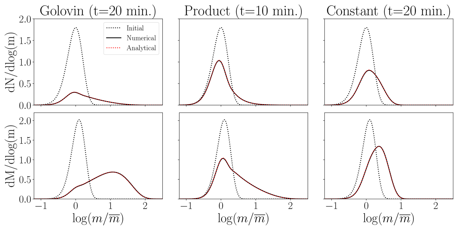
Figure 4 BinMod1D Jupyter notebook examples for the number (top row) and mass (bottom row) distribution functions with the Safronov/Golovin, product, and constant kernel (s_bin=32) with analytical solutions from Scott (1968) for μ₀=3 and Δt=1 s. Here, particle masses and mass distributions are normalized according to Scott (1968) such that the initial total number and total mass are both unity. The spectral_1d option moments=2 is used for all model runs.

Figure 5 shows examples of collisional breakup only and the steady-state balance of coalescence with breakup along with the analytical solutions from Feingold et al. (1988). In these cases, the mass distributions very closely match the analytical solutions. There are somewhat larger differences in the number distributions. However, it is important to realize that the validity of the Feingold et al. (1988) analytical solutions depend upon several assumptions. In particular, the Feingold solutions do not exactly preserve explicit mass conservation for each breakup event although it does conserve the overall total distribution mass. BinMod1D, by contrast, explicitly calculates each bin-pair interaction such that mass is always conserved for each interaction event regardless of the fragment distribution. In this way, BinMod1D represents a much more physically realistic way to explicitly simulate collisional breakup compared to the target-based method-of-moments models such as Feingold et al. (1988).

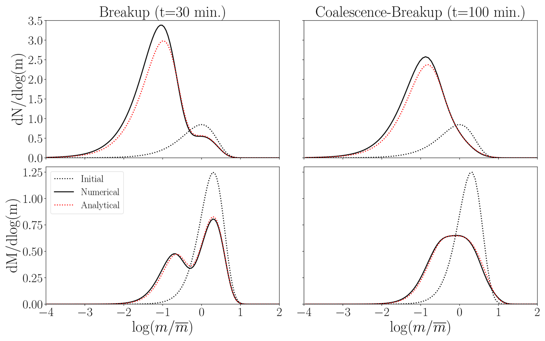
Figure 5 As in Fig. 4 but for the breakup (s=6, E_s=1.0, and E_b=0.1) and coalescence-breakup (s=4, E_s=0.8, E_b=1.0) constant kernel examples and analytical solutions from Feingold et al. (1988) assuming μ₀=0 and Λ_f=10 g⁻¹. The collision-coalescence and collisional breakup analytical solution is a steady-state solution.

3.2 Steady-state examples

Figure 6 shows two examples of the steady-state (i.e., height only) BinMod1D simulation for a rain case using the plot_moments_radar and plot_dists_height methods of the spectral_1d class. For these simulations, the initial distribution is given by $D_{m,\mathrm{0}}=\mathrm{0.8}$ mm, $N_{t,\mathrm{0}}=\mathrm{15}$ L⁻¹, and μ₀=0. A 3 km layer is considered here with ztop=3000., zbot=0., and Δz=10 m (dz=10.). For collision-coalescence only (E_s=0.8), number concentration and liquid water content (LWC) decrease with decreasing height whereas mean volume diameters increase with decreasing height. Similarly, Z, Z_DR, and K_dp all increase with decreasing heights as coalescence transfers mass from smaller sizes to larger sizes. This, in turn, increases raindrop sizes and decreases raindrop aspect ratios according to the Brandes et al. (2002) aspect ratio-diameter polynomial relationship. Figure 6 also shows the size distributions at 3.0, 1.5, and 0.0 km. As the size distributions evolve downward, the initial inverse-exponential distribution transitions to a more gamma-like shape.

Figure 6 also shows the same simulation but with the incorporation of breakup with E_b=0.005 and an exponential fragment distribution (frag_dist='exp'). By default, the mean volume diameter of frag_dist='exp' is 0.25 mm. The combined coalescence-breakup simulation overall is quite similar to the coalescence only simulation, however there is a noticable stagnation effect that is most obvious for D_m, liquid water content (LWC) and the radar variables. This stagnation effect results from the presence of breakup stunting the coalescence growth effects. The size distribution at 1.5 km is very similar to the coalescence only simulation, especially in the tail portion of the distribution. However, the exponential fragment distribution is clearly visible and becomes more pronounced at z=0.0 km.

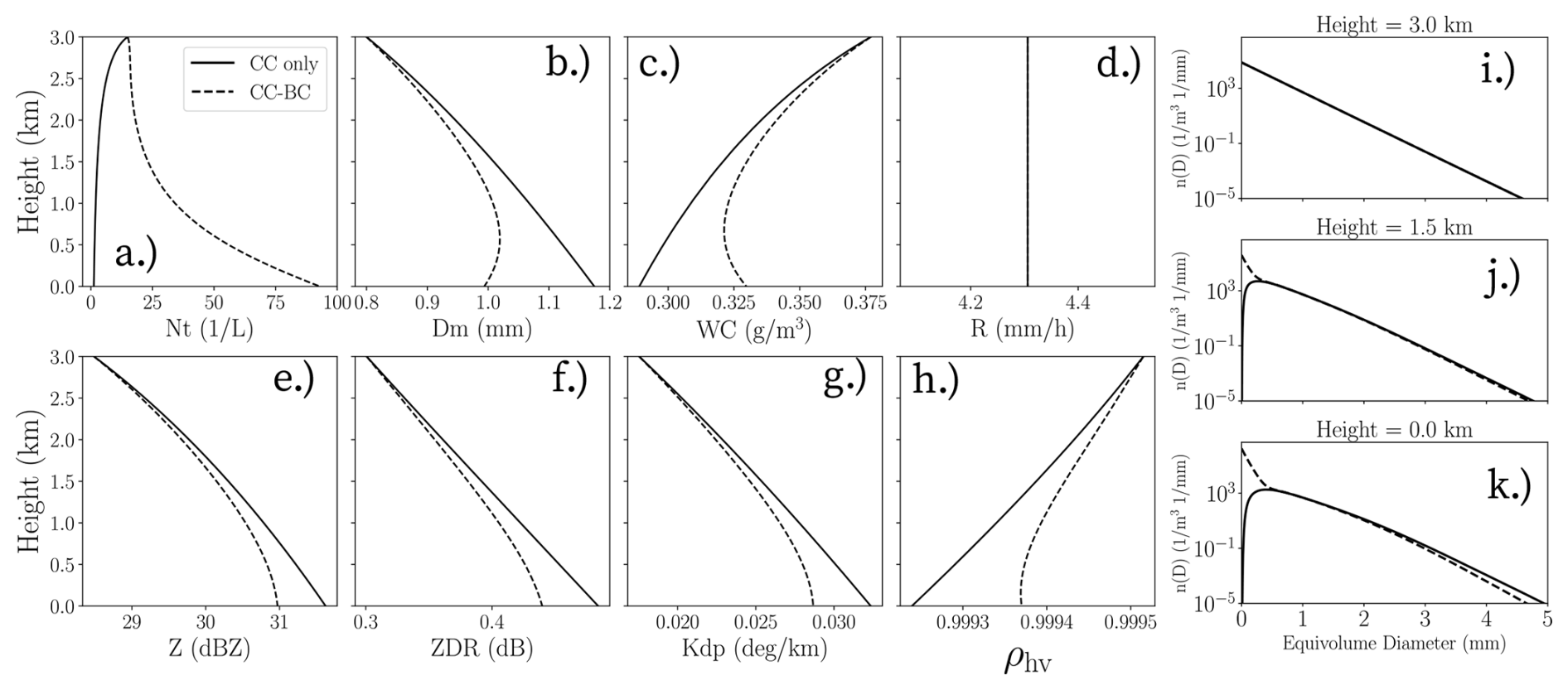
Figure 6 Various microphysical and radar variables for the steady-state rain example including: (a) Number concentration, (b) Mean volume diameter, (c) Liquid water content, (d) Rain rate, (e) Radar reflectivity, (f) Differential reflectivity, (g) Specific differential phase, and (h) Correlation coefficient. Solid lines represent the collision-coalescence only simulation (CC only) whereas dashed lines show the combined collision-coalescence/collisional-breakup (CC-BC) simulations. Subpanels (i) through (k) show the number distribution function at 3.0, 1.5, and 0.0 km, respectively.

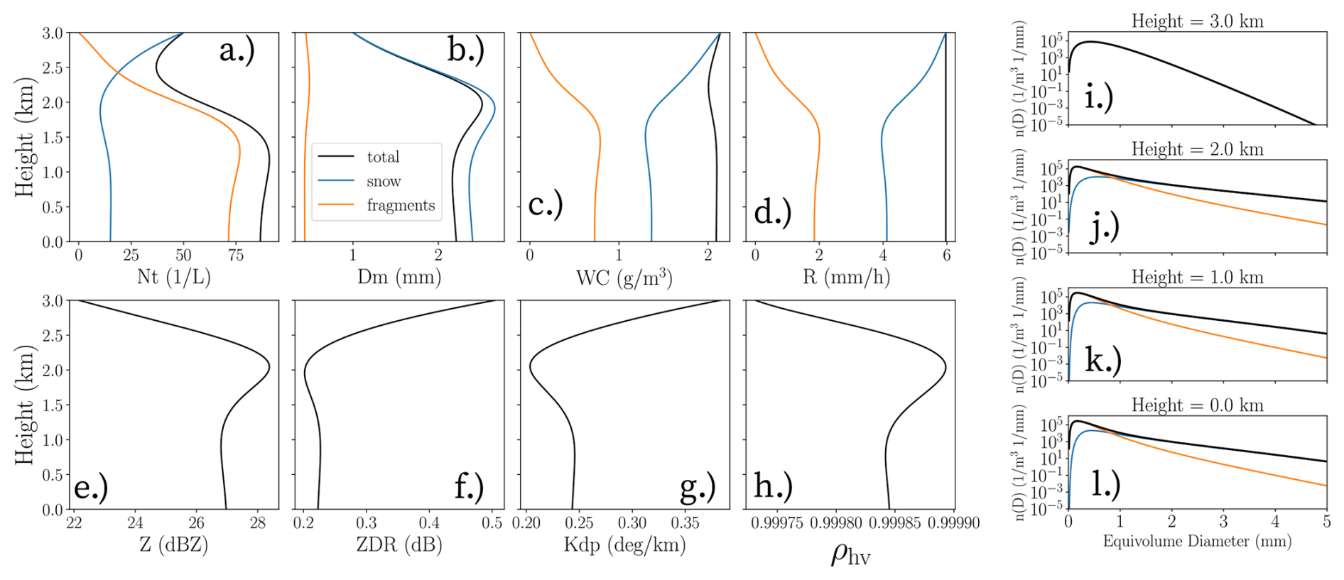
Figure 7 shows a steady-state example of snow aggregation and collisional breakup. This scenario can be thought of as the effects of aggregation and breakup below the dendritic growth layer (DGL). Many studies have investigated these polarimetric radar signatures (Kennedy and Rutledge, 2011; Andrić et al., 2013; Schrom et al., 2015; Griffin et al., 2018; Dunnavan et al., 2022) and it is well known that reflectivity typically increases downward below whereas differential reflectivity and specific differential phase typically decreases downward. Here, BinMod1D is run with an initial gamma distribution with $N_{t,\mathrm{0}}=\mathrm{50}$ L⁻¹, $D_{m,\mathrm{0}}=\mathrm{1.0}$ mm, and μ₀=3. Furthermore, two distinct category distributions are used: snow and fragments, where each sample distribution has microphysical parameters determined by the habits.py module (i.e., habit_params=['snow','fragments']). In particular, snow particles have a fixed aspect ratio of 0.6 with an orientation parameter of 0° (horizontal orientation) whereas fragments have aspect ratios of 0.8 and an orientation parameter of 20°. The simulation is also set up so that aggregated particles go to the snow distribution (cc_dest=1) whereas the breakup fragments go to the fragment distribution (br_dest=2) that is governed by an assumed lognormal distribution with a mode at D_mode=0.2 mm and a median of D_med=0.25 mm (i.e., frag_dist='LGN'). As shown in Fig. 7, the microphysical variables can be shown independently for each category when running spectral_1d with multiple distribution categories. This simulation shows the domination of aggregation from 3.0 to 2.0 km where reflectivity and D_m rapidly increase downward. From 2.0 to 1.0 km, breakup overwhelms aggregation which leads to a U-shaped reversal of the height profiles. Finally, 1.0 to 0.0 km shows a balance of aggregation with collisional breakup such that the total distribution and its bulk variables more-or-less stagnate. It is important to note that this stagnation effect is typically ignored in models as collisional breakup is often not explicitly taken into account.

Figure 7 As in Fig. 6 but for snow aggregation and collisional breakup as described in text. Here, s_bin=3 and Δz=5 m.

3.3 Full model examples

Figure 8 shows an example of a rain “fallout” when boundary=None. In this case, the same initial rain distribution from Sect. 3.2 is used but with E_col=1.0, E_s=0.25, s_bin=2, Δt=2 s, Δz=20 m, and 60 bins. With these parameters, this full simulation out to $t_{max}=\mathrm{1500}$ s takes about 50 s on a laptop (see Sect. 4 for more information regarding the laptop specifications). The initial inverse-exponential distribution is only in the top height grid box initially. As time progresses, the initial distribution both sediments and engages in collision-coalescence. Size sorting of drops in different bins accounts for the gradual spreading of the reflectivity signature as the largest drops land before smaller drops.

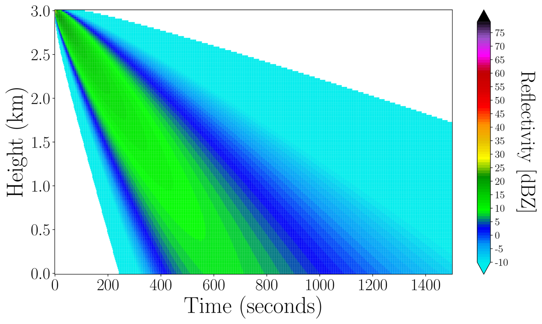
Figure 8 A time/height reflectivity profile (for a radar wavelength of 110 mm) for a rain fallout example where boundary=None.

Figure 9 shows a full 1D column model simulation for snow with aggregation (E_s=0.35) representing the DGL simulation from Sect. 3.2 but with slightly larger initial snow particles ($D_{m,\mathrm{0}}=\mathrm{1.25}$ mm). Unlike in the rain fallout example, here boundary='fixed' which indicates that the top particle size distribution (and therefore the topmost mass and number fluxes) is held constant. Therefore, this simulation will tend toward the steady-state solution as t→∞. As in the steady-state simulation, s_bin=2 with 60 total bins. The model is run with only one category out to 5400 seconds with Δt=2 s and Δz=20 m and an output frequency of 1 (i.e., every Δt timestep). The simulation itself takes just less than 5 min to run on the laptop used to conduct timing and convergence tests in Sect. 4. The radar time/height profiles in Fig. 9 show the classic aggregation signature of an increasing reflectivity and decreasing Z_DR and K_dp toward ground. The system itself evolves slower than the rain case due to the slower fall speeds as it takes slightly less than an hour for the largest snowflakes to reach the surface. The Z_DR time/height profile also shows the presence of size sorting as the larger, more oblate snowflakes reach the surface before the smaller, slower falling snowflakes. The simulation itself reaches a quasi steady-state after about 4000 s.

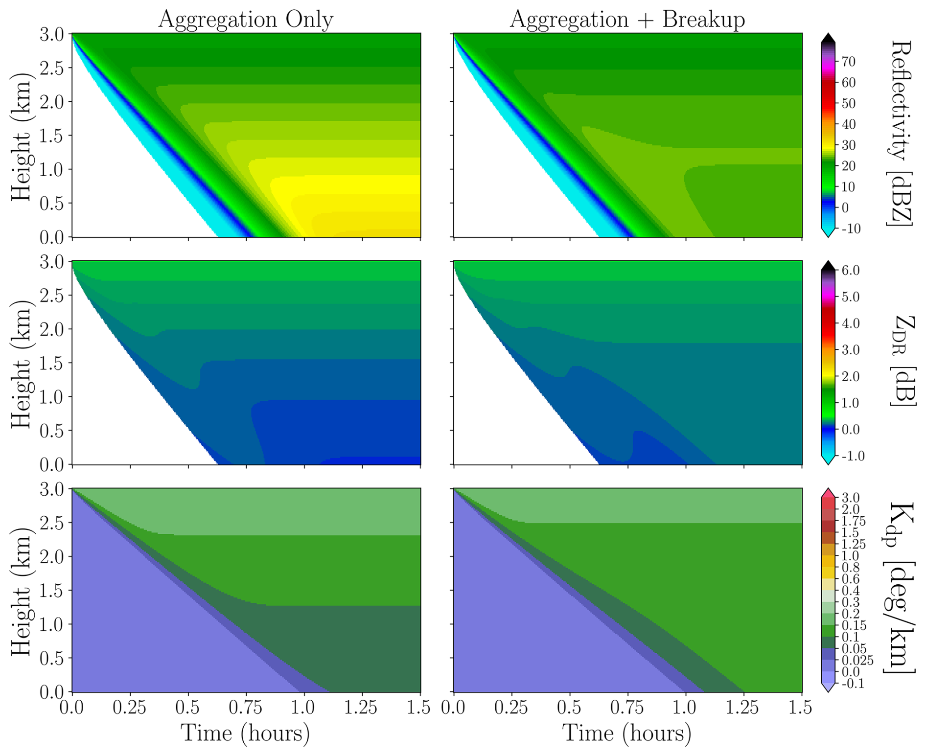
Figure 9 A snow aggregation example (left column) for reflectivity (top), differential reflectivity (middle), and specific differential phase (bottom) of BinMod1D where boundary=fixed. Right column represents the 2 category aggregation and breakup simulation.

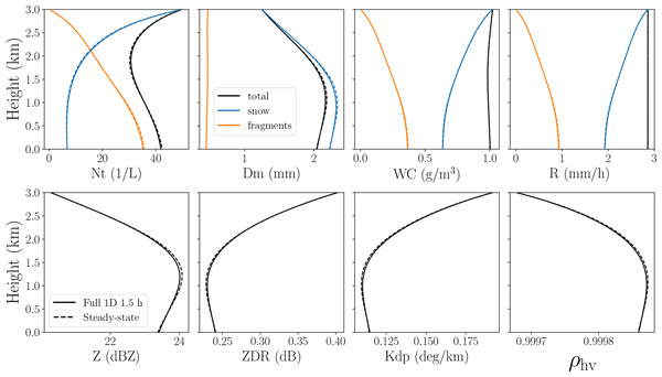
Figure 10 shows the results of the previous DGL simulation but with the addition of collisional breakup. As in the steady-state simulation, the default lognormal fragment distribution is used. However, here E_s=0.6 and E_b=0.05 and the full simulation took 26 min to run. Figure 10 shows that the moments and radar variables for the full 1D column model simulation at t=1.5 h is nearly identical to the corresponding steady-state simulation. The behavior of the profiles are also similar to Fig. 7 but where reflectivity maximizes at 1.0 km rather than 2.0 km. The corresponding time/height profiles are shown alongside the aggregation only results in Fig. 9. The simulations are very similar up until 2000 s where the presence of fragmentation begins to influence the radar fields. Although the start of the surface snowfall occurs at roughly the same time, the combined aggregation and breakup simulation produces a lower surface reflectivity than the aggregation only simulation. The presence of fragments also leads to a higher ZDR and K_dp which both stay very constant in the bottom 1.5 km of the model domain.

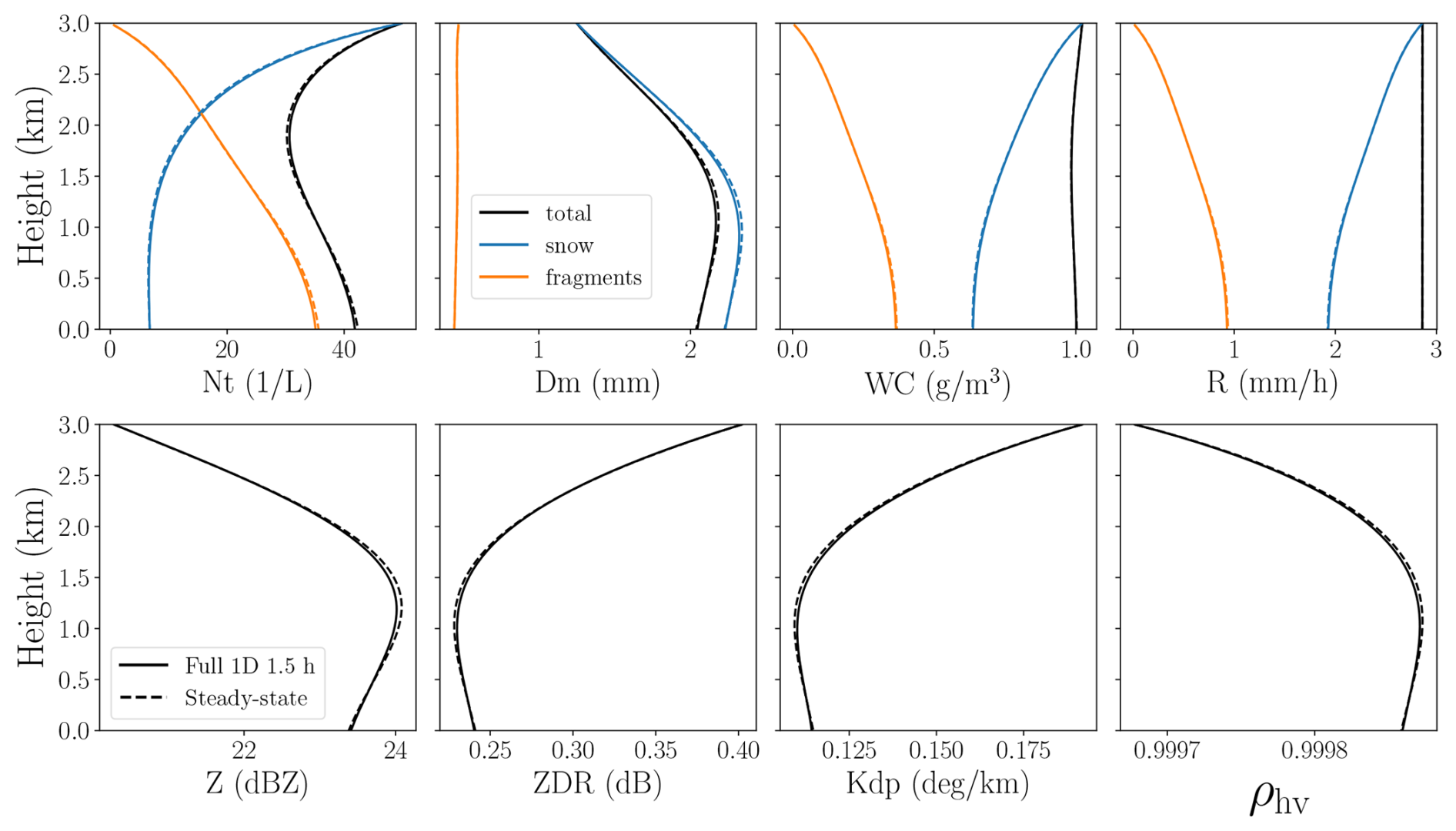
Figure 10 Moments and forward simulated radar variable comparison of a full time and height snow aggregation/breakup BinMod1D model run at t=1.5 h compared to the corresponding steady-state BinMod1D model run.

4 Accuracy, computational speed, and resolution

Timing tests are performed on a workstation laptop equipped with a 12th generation Intel(R) Core i7-12850HX processor (2.1 GHz and 16 cores) and 64 GB of RAM running in a standard Python environment. These specifications represent standard high-end consumer hardware, thereby demonstrating that the model can be effectively used without the need for specialized high-performance computing (HPC) resources.

These timing and convergence tests use the box model capability of BinMod1D to simulate a transition from continental cloud droplets to moderate rain with Z≈40 dBZ. This is similar to simulations performed by Simmel et al. (2002) and Wang et al. (2007). However, unlike those simulations, the BinMod1D simulations include both collision-coalescence and collisional breakup. Here, the precipitation type is considered to be rain with one category and the Best (1950) fall speed parameterization is used rather than the default Atlas and Ulbrich (1977) power-law parameterization. The Long kernel (kernel='Long') is used where the collision efficiency⁵ is given by (cf. Long, 1974; Simmel et al., 2002)

$$\begin{array}{}\text{(19)}& \begin{array}{rl}& E_{\mathrm{col}}=E_{\mathrm{col}}(x,y)\left[{\mathrm{mm}}^{\mathrm{3}}{\mathrm{s}}^{-\mathrm{1}}\right]=\\ & \left\{\begin{array}{ll}max\left[\mathrm{112.5}{D}_y^{\mathrm{2}}\left(\mathrm{1}-\frac{\mathrm{0.006}}{D_x}\right),\mathrm{0.001}\right]& D_y<\mathrm{0.1}\mathrm{mm}\\ \mathrm{1.0}& D_y\ge \mathrm{0.1}\mathrm{mm}\end{array}\right.\end{array}\end{array}$$

where D_x≥D_y and the hydrodynamic kernel is used such that

$$\begin{array}{}\text{(20)}& K_{\mathrm{hydro}}=E_{\mathrm{col}}{E}_{\mathrm{s}}{\displaystyle \frac{\mathit{\pi }}{\mathrm{4}}}{\left(D_x+D_y\right)}^{\mathrm{2}}\left|v_{t,x}-v_{t,y}\right|,\end{array}$$

and the sticking efficiency E_s is set to 0.6. The Straub et al. (2010) fragment distribution parameterization with E_b=1.0 (i.e., no rebounding) is used as well (frag_dist='Straub') which characterizes rain-rain fragments with a lognormal distribution, two Gaussian distributions, and a Dirac delta function for the residual rain drop. In order to prevent the breakup of cloud droplets, two linear ramp functions are used to scale E_b based on both the maximum size of the (i,j) collection pair diameter bin midpoints (1.2 mm < $max(D_i,D_j)$ < 2.8 mm) and based on the size ratio $\left[q\equiv min\left(D_i,D_j\right)/max\left(D_i,D_j\right)\right]$) between the collection pair diameter bin midpoints ($\mathrm{0.1}<q<\mathrm{0.25}$). Pairs with values less than the first edge have E_BR scaled by 0 (i.e., breakup is not considered) whereas pairs with values greater than the second edge values are scaled by unity (i.e., breakup is only scaled by E_BR as it is by default). In addition to the Long kernel being a more accurate representation of the autoconversion process for cloud droplets, previous studies such as Wang et al. (2007) have also found that more realistic kernels like the Long kernel can have a slower numerical convergence for different s_bin values than for less realistic kernels (i.e., Safronov/Golovin, product, constant, etc.). Furthermore, these tests are, generally speaking, much more numerically demanding than what most users will typically experience. There are a number of reasons for this. First, the initial distribution consists of a very large number concentration (𝒪(10⁵ L⁻¹)). This means that the number of binary interactions that occur at the beginning of the simulation is much greater than for simulations involving fully developed rain and snow. This also means that breakup requires adaptive stepping in order to ensure numerical stability.

In each test, a s_bin=16 value with two-moment calculations is used as the reference solution to determine the accuracy of the BinMod1D model runs. The results shown herein are similar to the box model results from Simmel et al. (2002) and Wang et al. (2007) where the initial distribution is a gamma distribution with μ=0 (i.e., an exponential distribution) and normalized according to mass similar to Scott (1968) but with ${\stackrel{\mathrm{‾}}{D}}_{\mathrm{0}}=\mathrm{18.6}$ µm and $M_{t,\mathrm{0}}=\mathrm{1}$ g m⁻³ (parameters consistent with both Simmel et al., 2002 and Wang et al., 2007). This leads to $N_{t,\mathrm{0}}\approx \mathrm{300}\mathrm{000}$ L⁻¹. In this sense, these convergence and timing tests are representative of continental cloud systems that transition from autoconversion of cloud droplets to accretion of cloud droplets by rain droplets and the resulting steady-state balance of coalescence and collisional breakup.

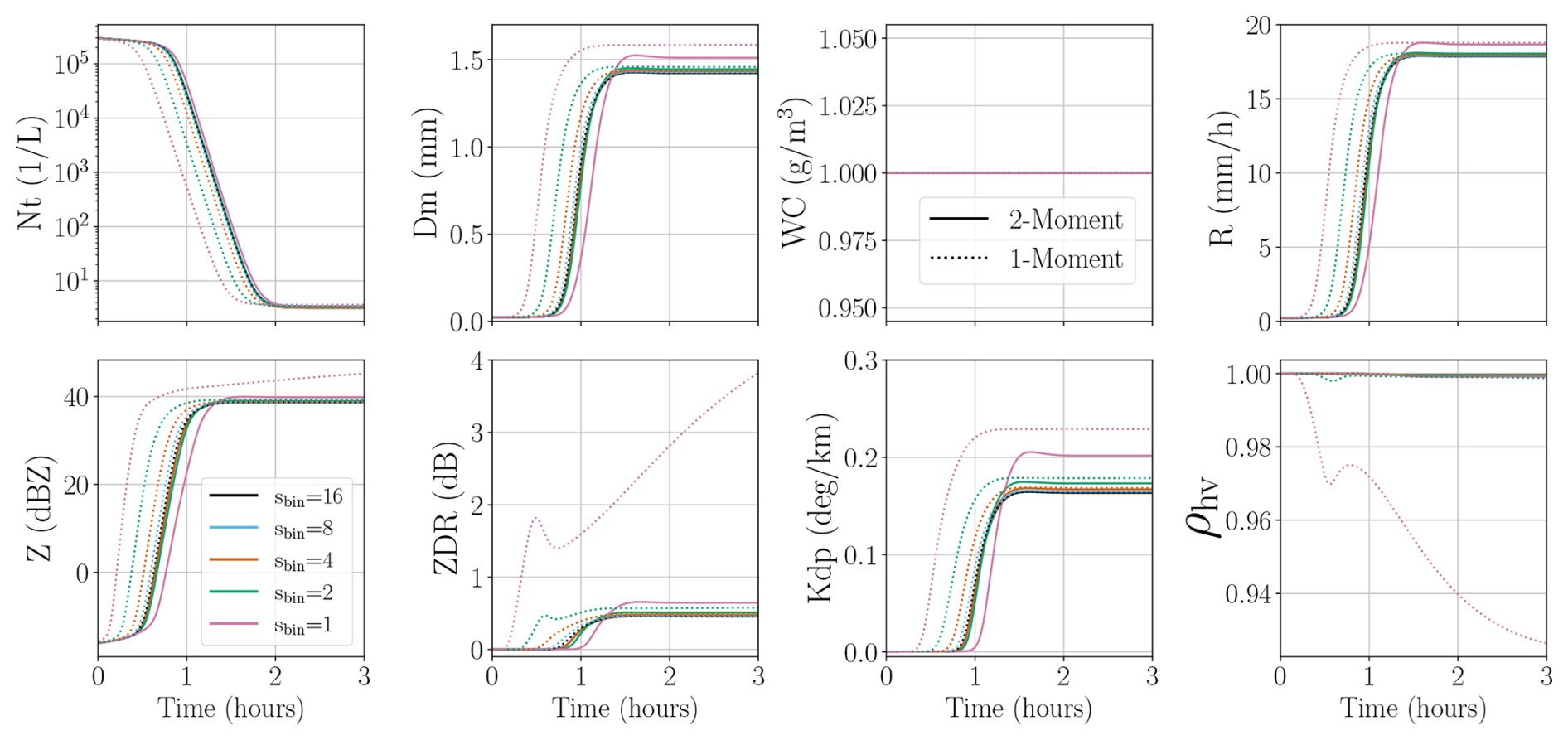
Figure 11 The timeseries evolution of number concentration, mean volume diameter, liquid water content, rain rates as well as radar reflectivity, differential reflectivity, specific differential phase, and correlation coefficient for cloud-rain convergence and testing simulations. Here, the radar wavelength is 110 mm which is consistent with S band radars. Each simulation uses Δt=1 s and an output frequency of 10 s.

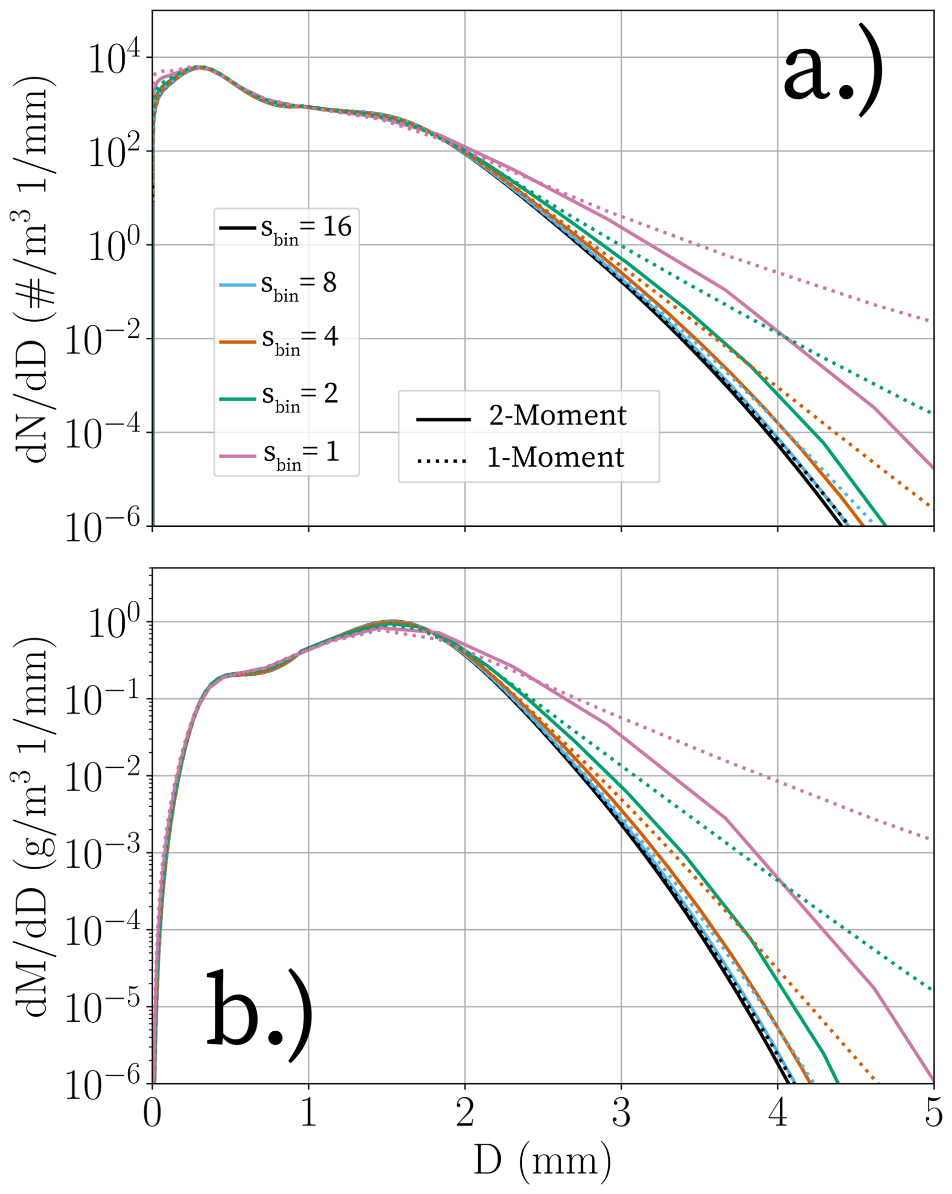
Figure 12 Number (a) and mass (b) distribution functions from the box model simulations at 3 h for different s_bin parameters and for 2-moment simulations (solid lines) and 1-moment simulations (dotted lines).

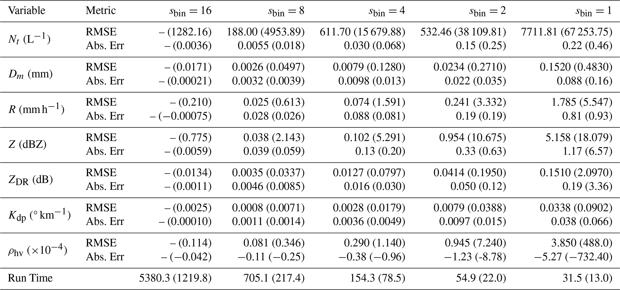
Figure 11 shows the timeseries of microphysical and radar variables for each simulation. Each simulation, regardless of resolution or moment prediction, produces the same qualitative behavior in the 3 h period. Initially, autoconversion of cloud droplets is gradual and the distributions do not change much. For the reference solution s_bin=16 and moments=2, it is clear that it takes roughly 40 min for accretion to finally become dominant. However, the one-moment simulations struggles to capture this delay effect and instead accelerates the accretion process sooner. This is primarily because the collision-coalescence and collisional breakup processes are very sensitive to number concentration as the number of collisions increases rapidly with number concentration. The explicit prediction of number concentration with the two-moment simulations offsets this rapid acceleration and produces the correct transition point even with a somewhat coarse s_bin=2 value. The s_bin=1 with moments=2 simulation actually over-delays the autoconversion-accretion process slightly. As shown in Table 1, the root-mean-square (RMSE) errors for BinMod1D one-moment number concentrations with s_bin=16 (1282.16 L⁻¹) is actually more than twice as large as the BinMod1D two-moment number concentrations with s_bin=2. Despite this, the absolute errors of number concentration at 3 h is overall quite low for all simulations where the maximum error is only 0.46 L⁻¹ for s_bin=1 and moments=1 for a reference value of 3.17 L⁻¹ from the s_bin=16 and moments=2 simulation. This behavior is consistent with the other microphysical variables as well. Even the coarse bin resolution s_bin=1 two-moment model run leads to only a slight overestimation of N_t, D_m, and R by 0.22 L⁻¹, 0.088 mm and 0.81 mm h⁻¹, respectively. Similarly, Z, Z_DR, and K_dp are within 1.17 dBZ, 0.19 dB, and 0.038 ° km⁻¹ of the s_bin=16 reference solution, respectively.

The radar variables, particular the polarimetric ones, show more sensitivity. The diffusive nature of the one-moment solutions exacerbates the accelerated autoconversion-accretion transition shown in the reflectivity timeseries due to the D⁶ weighting. As a result, the s_bin=1 with moments=1 simulation almost immediately increases rapidly with reflectivity and differential reflectivity whereas specific differential phase has a slightly longer apparent transition period. Most notably the s_bin=1 with moments=1 simulation dramatically overestimates the Z_DR by 3.36 dB and underestimates ρ_hv by 0.0732. These exaggerated values are due to the extreme diffusion at the large end of the particle mass distribution (Fig. 12) which shows a near exponential behavior with size rather than the super-exponential behavior from collisional breakup that the more accurate, higher resolution simulations show. Increasing s_bin from 1 to 2 noticeably improves this diffusive behavior much closer to the reference solutions. Overall, even s_bin=2 with moments=2 faithfully captures the correct timeseries of each variable and the correct bimodal steady-state number and mass distribution functions at 3 h. Run times range from 13 s for the coarsest run to 5380 s for the reference simulation. However, even the second highest resolution run (s_bin=8 for moments=2) only takes slightly longer than 10 min to perform on a laptop computer. As stated before, these simulations are typically much more demanding than what most users will experience due to the large initial number concentration and the adaptive stepping needed to accurately simulate breakup for these large number of interactions.

Table 1 Timing and convergence tests of BinMod1D. For each variable, the top row represents RMSE and the bottom row represents the absolute error at 3 h. Numbers in parentheses indicate 1-moment runs; those without represent 2-moment runs.

5 Conclusions

BinMod1D is a simple, economic spectral bin microphysics model that should be accessible for those familiar with the Python programming language. Other similar Python packages like LCM1D and PySDM use Lagrangian depictions of the PSD evolution rather than the typical Eulerian description given by traditional spectral bin microphysics schemes. In this way, BinMod1D represents a much more traditional approach that is more similar to the widely-used Fast Spectral Bin Microphysics scheme (FSBM; Khain and Lynn, 2009) which is available in the Fortran-based Weather Research and Forecasting (WRF) model. BinMod1D provides an expedient way to not only generate box model or 1D column model PSD evolution due to coalescence and/or breakup, but also to easily incorporate various habit parameters, numbers of distributions, and interaction kernels. Additionally, BinMod1D, unlike other similar Python packages, allows for direct, explicit simulation of steady-state vertical radar profiles. This article provides only a small set of examples for using the model. However, due to its flexibility, BinMod1D can be customized for a variety of different purposes. For example, users could use BinMod1D to perform in-situ-type bin model simulations similar to Field et al. (2006) where actual in-situ-derived particle size distributions are used to initialize the bin model and investigate the theoretical effects of aggregation (and/or breakup) compared to measured distributions taken from such Lagrangian aircraft spirals. Similarly, users could also develop theoretical particle size distributions valid for laboratory studies such as done in Connolly et al. (2012).

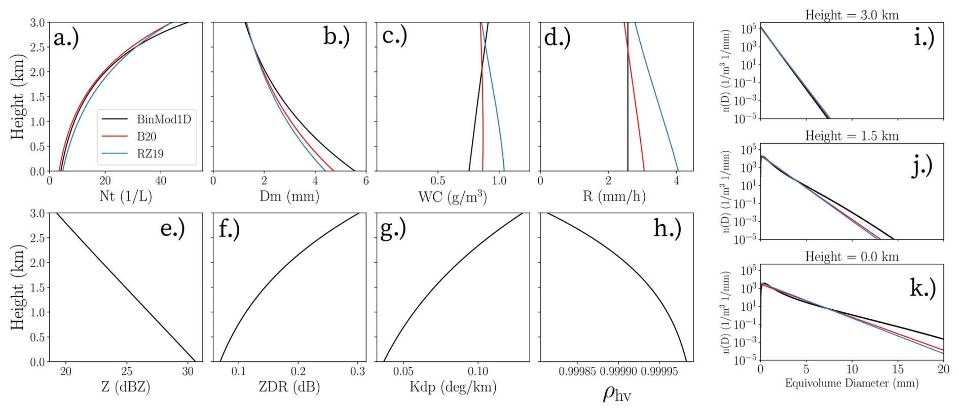
Figure 13 BinMod1D (black lines) steady-state results for a heavy snow case. Panels (a) through (d) and (i) through (k) also show corresponding retrievals using the Bukovčić et al. (2020) (B20; red lines) and Ryzhkov and Zrnić (2019) (RZ19; blue lines) power law relations.

Figure 13 presents another possible application: retrieval methodology validation. In this example, BinMod1D is run in the steady-state mode to produce synthetic snow size distributions in height. Here, s_bin=6 with 180 bins in order to produce a high resolution set of PSDs. This simulation uses an initial exponential distribution with parameters $N_{t,\mathrm{0}}=\mathrm{50}$ L⁻¹ and $D_{m,\mathrm{0}}=\mathrm{1.25}$ mm which produces an initial reflectivity of about 20 dBZ. E_s=0.35 is used to simulate the explicit steady-state PSD evolution in height due only to aggregation. This increases the reflectivity to approximately 30 dBZ at the surface. The $Z/K_{\mathrm{dp}}$ Bukovčić et al. (2020) (B20) and the $Z/Z_{\mathrm{DR}}/K_{\mathrm{DP}}$ Ryzhkov and Zrnić (2019) (RZ19) power-law retrievals are then used to retrieve N_t, D_m, IWC, and R solely from the BinMod1D polarimetric radar height signatures (see Table 1 from Dunnavan et al., 2022, for these retrieval equations). In this way, these comparisons shows the limitations of these retrieval methods due to using a fixed distribution shape. The BinMod1D simulation and Ryzhkov and Zrnić (2019) retrievals assumes the same snow parameters as used in Bukovčić et al. (2020) to derive their retrievals where the snow aspect ratios are 0.65, σ=0°, the density-size power-law relation is $\mathit{\rho }\left(D\right)=\mathrm{0.178}{D}^{-\mathrm{1}}$, and the fall speed-size relation is v_t(D)=0.81D^0.15. Both sets of retrievals assume μ=0 for all heights. Initially, the retrieved size distribution parameters (Fig. 13a, b) are within 5 L⁻¹ and 0.05 mm of the initial BinMod1D exponential distribution N_t and D_m, respectively. The initial differences between the BinMod1D microphysical variables are due to the capping of the density at 0.92 g cm⁻³ at small sizes which the analytical retrieval formulas do not consider (for the retrievals to be simple power-law formulas, $\mathit{\rho }(D\to \mathrm{0})=\mathrm{\infty }$). Both B20 and RZ19 demonstrate the same general behavior of N_t(z) and D_m(z) from the explicit BinMod1D steady-state simulation. However, both retrievals underestimate the increase in D_m due to aggregation toward ground by nearly 1.0 mm. Figure 13 panels (i) through (k) shows that this is due to the retrievals tendency to approximate the quasi-exponential behavior in the millimeter size range but underestimate the size distribution of large aggregates present in the centimeter range. These sparse but large aggregates that generate in the BinMod1D simulation overall heavily weights the D_m calculation. Both B20 and RZ19 overestimate the snow rates particularly at the surface where both retrievals overestimate the size distribution in the mid-millimeter range (Fig. 13k). Figure 13c show that B20 retrieves a near constant IWC profile whereas RZ19 retrieves an IWC profiles that increases toward ground unlike the slightly decreasing IWC profile from BinMod1D. Overall, while the retrievals exhibit the correct overall behavior, these retrievals are still fundamentally limited by their inability to account for a changing distribution shape due to aggregation. This is one example where the reference solution provided by BinMod1D could be used to improve the retrieval equations of B20, RZ19, and others. Similarly, BinMod1D reference solutions can also be used to train retrieval-based artificial intelligence models.

There are a number of planned future improvements to the BinMod1D package including but not limited to

1. T-matrix radar forward simulation calculations.

2. Additional microphysical processes such as riming, melting, vapor deposition, condensation, evaporation, sublimation, and refreezing.

3. Incorporating non-constant coalescence and breakup efficiency parameterizations.

4. Incorporation of mixed-phase species (i.e., melting snow).

5. Incorporation of additional detailed collision-coalescence parameterizations including those of Phillips et al. (2015, 2017) for snow aggregation and collisional breakup.

6. The ability to specify a user-prescribed time-dependent top boundary condition for the boundary input parameter or an initial set of distributions in height.

7. Variable order Weighted Essentially Non-Oscillatory (WENO) advection calculations.

8. Ability to run the model using GPUs via the CuPy package (Okuta et al., 2017).