A continuous implicit neural representation framework with gradient regularization for sea surface height reconstruction from satellite altimetry

Satellite altimetry provides valuable measurements of sea surface height (SSH) but is characterized by irregular spatiotemporal sampling and substantial data gaps arising from orbital configurations, sensor limitations, and environmental conditions. These sampling properties pose challenges for constructing continuous and dynamically consistent SSH fields. In this study, we develop a reconstruction framework based on implicit neural representations (INRs), in which SSH is represented as a continuous function of space and time. The framework uses a sinusoidal representation network (SIREN)-based coordinate network to learn a continuous space–time representation of SSH from sparse along-track observations, and includes total-variation (TV)-based spatial-gradient regularization to discourage unsupported local variations. The combination of a continuous, differentiable INR formulation with gradient-based regularization provides a compact and flexible approach for SSH reconstruction. We evaluate the proposed framework using both multi-mission satellite altimetry observations and high-resolution numerical simulations. Experiments conducted indicate that the proposed SIREN–TV framework can reconstruct the broad SSH variability and dominant mesoscale patterns while reducing some localized reconstruction artifacts. The method maintains a level of global accuracy comparable to existing interpolation and data-assimilation approaches and provides improved effective feature resolution under the adopted benchmark protocol. In addition, the continuous and fully differentiable representation enables direct computation of spatial derivatives, facilitating higher-order oceanographic diagnostics. These results suggest that INR-based formulations offer a promising complementary avenue for SSH interpolation under sparse and irregular sampling configurations.

1 Introduction

Satellite altimetry provides the primary observational foundation for estimating sea surface height (SSH), a key variable for understanding ocean circulation, sea-level variability, and large-scale climate processes. Gridded SSH products derived from satellite altimetry are widely used in oceanographic research, supporting analyses of mesoscale and submesoscale dynamics and their role in the global ocean energy budget (Srinivasan and Tsontos, 2023). However, satellite altimeters measure SSH only along their ground tracks, and the resulting observations are sparse and irregular in space and time. Instrumental limitations, atmospheric effects, and orbital configurations can further lead to sampling gaps and uneven data coverage (Fablet et al., 2021). These limitations pose significant challenges for reconstructing continuous SSH fields that remain consistent with incomplete observations while preserving small-scale spatial variability (Shi and Jin, 2024).

Over the past decades, numerous algorithmic approaches have been developed to address the SSH mapping problem. The Data Unification and Altimeter Combination System (DUACS) represents the most established operational framework, relying on space–time optimal interpolation (OI) to merge multi-mission altimeter observations into gridded products (Le Traon and Dibarboure, 1999). DUACS provides robust large-scale SSH estimates and has been widely used in oceanographic applications. Nevertheless, the linear statistical formulation of OI tends to smooth localized mesoscale and submesoscale structures, such as fronts and eddy-related signals (Stegner et al., 2021). To improve the representation of fine-scale dynamics, several methods have introduced dynamical constraints into SSH mapping. For example, dynamical optimal interpolation (DOI) incorporates a constraint based on potential vorticity conservation into the interpolation procedure (Ubelmann et al., 2015), while the back-and-forth nudging approach based on quasigeostrophic dynamics (BFN-QG) uses dynamical information during assimilation to enhance SSH reconstruction (Le Guillou et al., 2021). Despite these advances, improving the effective resolution and spatial consistency of gridded altimetry products remains an ongoing challenge.

In recent years, data-driven and artificial intelligence (AI)-based methods have been increasingly applied to oceanographic problems. Preliminary studies have shown their potential for reconstructing and predicting sea surface conditions from partial and noisy satellite observations (Manucharyan et al., 2021; Lou et al., 2023; Camargo et al., 2023; Denvil-Sommer et al., 2023). The basic idea of data-driven interpolation is to estimate unknown values from patterns and statistical relationships learned from training data, rather than relying solely on prescribed interpolation rules or simplified assumptions. Despite these advances, many existing approaches still rely on discrete grid-based representations, in which the reconstructed field is defined on predefined spatial and temporal sampling intervals. This representation can limit the flexibility of the reconstruction when the observations are sparse, irregular, and not naturally aligned with the target grid.

To overcome the limitations of discrete grid-based formulations, implicit representations have emerged as an alternative framework for modeling continuous fields. Instead of storing values only at fixed grid points, an implicit representation models a field as a continuous function that maps coordinates to signal values. This coordinate-based formulation allows the field to be queried at arbitrary locations and times, making it suitable for reconstructing continuous spatial or spatio-temporal signals. Recent advances in computer vision and graphics have demonstrated that fully connected neural networks can serve as continuous and memory-efficient implicit representations for geometric entities such as shape components (Genova et al., 2019), objects (Oechsle et al., 2019), and scenes (Sitzmann et al., 2019). These models, known as implicit neural representations (INRs), parameterize continuous functions using multilayer perceptrons (MLPs) that learn coordinate-to-value mappings for complex spatial or spatio-temporal signals (Xu et al., 2022).

Beyond their conceptual simplicity, INRs possess several properties that make them attractive for scientific field reconstruction. Because they are defined as functions of coordinates, INRs can represent a continuous field without being restricted to a fixed output grid. Their differentiable formulation also allows gradients and higher-order derivatives to be computed through automatic differentiation, which is useful when derivative-based constraints or diagnostics are needed. As a result, INRs have been successfully applied to shape modeling (Ye et al., 2022), texture synthesis (Guan et al., 2023), inverse problems (Molaei et al., 2023), and generative modeling (Wiesner et al., 2022). However, their adoption in the Earth sciences remains limited, particularly in oceanographic reconstruction problems. Motivated by these advantages, this study leverages INRs to represent SSH as a continuous function of spatial and temporal coordinates from sparse satellite altimetry observations.

The performance of an INR depends strongly on the choice of network architecture. Conventional coordinate-based MLPs may have difficulty representing fine-scale or rapidly varying components. Fourier feature mappings have been used to enhance the representation of high-frequency details, but they may introduce noisy or unstable gradients in some applications (Tancik et al., 2020). The Sinusoidal Representation Network (SIREN) offers another solution by using sine activation functions in fully connected networks (Sitzmann et al., 2020). The sinusoidal activation provides a smooth and differentiable coordinate-based representation, which is suitable for continuous fields with spatial and temporal variability. For SSH reconstruction, this property is useful because the target field contains both broad large-scale variations and localized mesoscale structures that may appear as relatively sharp spatial gradients. In this study, we adopt SIREN as the INR backbone for representing SSH as a continuous function of spatial and temporal coordinates from sparse satellite altimetry observations.

However, when a SIREN-based INR is trained only with a data-fidelity loss, the reconstruction is directly constrained only at the observed along-track locations. In regions with large gaps between satellite tracks or low local observation density, a data-fidelity loss alone provides little constraint on how SSH should vary between tracks. The learned SSH function may therefore introduce small-scale fluctuations that are not well supported by nearby observations; in the reconstructed field, these fluctuations appear as rapid SSH changes over short spatial distances and are reflected by large local spatial gradients. To reduce such variations, we incorporate a total variation (TV)-based spatial-gradient regularization term into the SIREN-based INR framework. The proposed framework contains two main components. First, a SIREN-based implicit representation is used to represent SSH as a continuous function of spatial and temporal coordinates from sparse altimetry observations. Second, a spatial-gradient TV regularization term is added to the training objective to penalize excessive local spatial gradients in the reconstructed field. In this way, the model is encouraged to remain consistent with the available along-track measurements while reducing unsupported small-scale fluctuations that may arise under sparse and irregular satellite sampling.

The remainder of this paper is organized as follows. Section 2 introduces the background of implicit neural representations and their relevance to continuous field reconstruction. Section 3 formulates the SSH reconstruction problem from sparse satellite altimetry observations. Section 4 presents the proposed reconstruction framework, including the SIREN-based implicit representation, coordinate normalization, and TV-based spatial-gradient regularization. Section 5 reports the experimental results using both real satellite altimetry observations and simulated SSH fields. Section 6 discusses the methodological characteristics, limitations, and applicability of the proposed framework. Finally, Sect. 7 concludes the paper.

2 Background: implicit neural representations

Implicit neural representations (INRs) provide a way to describe a continuous field as a function of its coordinates. Instead of assigning values only to a finite set of locations, an INR learns a coordinate-to-value mapping that can be queried at arbitrary positions within the domain. This idea is useful for geophysical reconstruction problems, where observations are often sparse or irregular, but the target variable is expected to vary continuously in space and time.

In an INR, the input coordinate is passed through a coordinate-based multilayer perceptron. Let s denote a general input coordinate. The neural representation is written as Φ_θ(s), where θ denotes the trainable network parameters and Φ_θ gives the field value at the queried coordinate. In a standard coordinate-based MLP, each hidden layer applies an affine transformation followed by a nonlinear activation:

$$\begin{array}{}\text{(1)}& {\mathit{z}}_{i+\mathrm{1}}={\mathit{\sigma }}_i({\mathbf{W}}_i{\mathit{z}}_i+{\mathit{b}}_i),{\mathit{z}}_{\mathrm{0}}=\mathit{s}.\end{array}$$

The final layer maps the last hidden representation to the reconstructed SSH value.

Because Φ_θ is defined as a function of the input coordinate, the trained model can be evaluated at any coordinate within the study domain. For SSH reconstruction, this means that the learned function can estimate sea surface height not only at observed satellite-track locations, but also at unobserved longitude–latitude–time coordinates. This coordinate-based property makes INRs a suitable representation tool for reconstructing spatially and temporally complete SSH fields from sparse altimetry observations.

3 Problem formulation

Satellite radar altimeters measure SSH only along their ground tracks, resulting in sparse and irregular spatio-temporal observations. Let $\mathit{s}=(\text{lon},\text{lat},\text{time})$ denote a general spatio-temporal coordinate, where lon, lat, and time represent longitude, latitude, and time, respectively. The coordinate of the ith satellite observation is denoted by ${\mathit{s}}_i=({\text{lon}}_i,{\text{lat}}_i,{\text{time}}_i)$, and the corresponding observed SSH value is denoted by SSH_true,i. The observation dataset is written as

$$\begin{array}{}\text{(2)}& \mathcal{D}=\mathit{\left\{}\right({\mathit{s}}_i,{\text{SSH}}_{\text{true},i}){\mathit{\}}}_{i=\mathrm{1}}^N.\end{array}$$

The goal of SSH reconstruction is to estimate a continuous SSH field over the study domain from these sparse along-track observations. In this work, the reconstructed field is represented as a coordinate-dependent function, so that an SSH value can be obtained for any given longitude–latitude–time coordinate within the reconstruction domain. At the observed coordinates, the reconstructed values should be consistent with the available satellite measurements. For locations away from the observed tracks, however, the SSH field must be inferred from the learned function of longitude, latitude, and time rather than by direct observations.

Because satellite altimetry provides sparse and irregular along-track measurements, the SSH field away from the observed tracks must be inferred from the learned function of longitude, latitude, and time rather than directly constrained by observations. Such a reconstruction may contain unsupported local fluctuations, which motivates the use of spatial regularization in the proposed framework.

4 Proposed framework

This section presents the proposed INR-based framework for reconstructing a continuous SSH field from sparse satellite altimetry observations. The approach combines a SIREN-based implicit neural representation with TV-based spatial-gradient regularization. The following Sections describe the coordinate normalization, network architecture, spatial-gradient regularization, and training objective.

4.1 SIREN-based implicit neural representation

The first component of the proposed framework is a SIREN-based INR for representing SSH as a continuous function of longitude, latitude, and time. For a given spatio-temporal coordinate $\mathit{s}=(\text{lon},\text{lat},\text{time})$, the network is designed to output the corresponding reconstructed SSH value. In geophysical terms, the network learns a function of longitude, latitude, and time that returns SSH from the available satellite-track samples. After training, this function is evaluated over the prescribed reconstruction domain and time window. In the present experiments, it is used to estimate SSH at target space–time coordinates in this domain, including locations and times not directly sampled by the satellite tracks. Thus, the continuous coordinate-based formulation provides interpolation within the sampled reconstruction problem, rather than implying unconstrained extrapolation to unrelated regions or periods. Before being passed to the SIREN network, the coordinate s is converted into a normalized coordinate, as described below.

4.1.1 Coordinate normalization

The input variables in SSH reconstruction have different physical units and numerical ranges. Longitude and latitude are measured in degrees, whereas time is measured in days. If these raw coordinates are directly used as network inputs, the difference in numerical scale may make the training less stable. Therefore, each coordinate is shifted and rescaled before being passed to the network:

$$\begin{array}{}\text{(3)}& \begin{array}{rl}{\displaystyle }& {\displaystyle }\stackrel{\mathrm{̃}}{\text{lon}}={\text{factor}}_{\mathrm{s}}\text{lon},\stackrel{\mathrm{̃}}{\text{lat}}={\text{factor}}_{\mathrm{s}}\text{lat},\\ {\displaystyle }& {\displaystyle }\stackrel{\mathrm{̃}}{\text{time}}={\text{factor}}_{\mathrm{t}}\text{time}.\end{array}\end{array}$$

The spatial scaling factor factor_s and temporal scaling factor factor_t are used to bring the spatial and temporal inputs to comparable numerical ranges. The normalized coordinate is denoted by $\stackrel{\mathrm{̃}}{\mathit{s}}=(\stackrel{\mathrm{̃}}{\text{lon}},\stackrel{\mathrm{̃}}{\text{lat}},\stackrel{\mathrm{̃}}{\text{time}})$.

This normalization is only a preprocessing step for the network input and does not change the physical meaning of longitude, latitude, or time. This preprocessing improves numerical conditioning and makes SIREN training more stable for the sparse multi-mission altimetry data used here.

4.1.2 Network architecture

After coordinate normalization, the normalized coordinate $\stackrel{\mathrm{̃}}{\mathit{s}}$ is used as the input to the SIREN network. Starting from the general INR layer in Eq. (1), we use a sinusoidal activation function to construct the hidden layers. Let ${\mathit{z}}_{\mathrm{0}}=\stackrel{\mathrm{̃}}{\mathit{s}}$ denote the input to the network. For the kth hidden layer, the layer output is defined as

$$\begin{array}{}\text{(4)}& {\mathit{z}}_{k+\mathrm{1}}=\sin ({\mathbf{W}}_k{\mathit{z}}_k+{\mathit{b}}_k),k=\mathrm{0},\mathrm{\dots },L-\mathrm{1},\end{array}$$

where k denotes the hidden-layer index, L is the number of hidden layers, W_k and b_k are the trainable weights and biases of the kth hidden layer, and the sine function is applied element-wise. Here, k=0 corresponds to the first hidden layer, and $k=L-\mathrm{1}$ corresponds to the last hidden layer. Compared with the general form in Eq. (1), Eq. (4) specifies the activation function as sin (⋅).

We employ a fully connected SIREN network consisting of an input layer, several sinusoidal hidden layers, and a final linear output layer. After the last hidden layer, the reconstructed SSH value at the queried coordinate is obtained as

$$\begin{array}{}\text{(5)}& {\mathrm{\Phi }}_{\mathit{\theta }}\left(\stackrel{\mathrm{̃}}{\mathit{s}}\right)={\mathbf{W}}_{\text{out}}{\mathit{z}}_L+{\mathit{b}}_{\text{out}},\end{array}$$

where z_L is the last hidden representation, and W_out and b_out are the parameters of the output layer. The parameter set θ includes all hidden-layer weights and biases as well as the output-layer parameters. The differentiability of this coordinate-based representation is used in the spatial-gradient regularization introduced below.

4.2 TV-based spatial-gradient regularization

The second component of the proposed framework uses normalized-coordinate gradients of the reconstructed SSH field to reduce unsupported rapid local variations. Since the SIREN-based INR is differentiable with respect to its normalized input coordinates, these derivatives can be computed with respect to normalized longitude and latitude. They are used only to define the dimensionless TV regularization term below and are not interpreted as physical SSH gradients per unit distance.

4.2.1 Data-fidelity loss

The data-fidelity loss measures the mismatch between the observed SSH value and the reconstructed SSH value at each satellite-track location. For an observed coordinate s_i, let SSH_true,i denote the satellite-observed SSH value and let ${\text{SSH}}_{\text{rec},i}={\mathrm{\Phi }}_{\mathit{\theta }}\left({\stackrel{\mathrm{̃}}{\mathit{s}}}_i\right)$ denote the reconstructed SSH value output by the network. The data-fidelity loss adopts the mean squared error:

$$\begin{array}{}\text{(6)}& {\mathcal{L}}_{\text{data}}\left(\mathit{\theta }\right)={\displaystyle \frac{\mathrm{1}}{N}}\sum _{i=\mathrm{1}}^N{\left({\text{SSH}}_{\text{rec},i}-{\text{SSH}}_{\text{true},i}\right)}^{\mathrm{2}}.\end{array}$$

This term constrains the network output SSH_rec,i to match the observed value SSH_true,i at the available satellite-track locations. The unweighted mean squared error can also be related to a standard least-squares interpretation, in which the available along-track observations are treated with a common error variance. Thus, the present experiments use an ordinary least-squares data term in which the observed along-track samples contribute equally.

However, the summation in Eq. (6) only includes observed coordinates where satellite measurements are available. For unobserved locations, there is no corresponding SSH_true value to directly guide the reconstruction. Under sparse and irregular sampling, the learned SSH function may therefore produce unsupported local variations. In the reconstructed field, such variations can appear as rapid SSH changes over short spatial distances and are reflected in large local spatial gradients.

4.2.2 Normalized-coordinate gradients for TV regularization

Let ${\mathrm{\Phi }}_{\mathit{\theta }}\left(\stackrel{\mathrm{̃}}{\mathit{s}}\right)$ denote the reconstructed SSH field. The normalized spatio-temporal coordinate is

$$\stackrel{\mathrm{̃}}{\mathit{s}}=(\stackrel{\mathrm{̃}}{\text{lon}},\stackrel{\mathrm{̃}}{\text{lat}},\stackrel{\mathrm{̃}}{\text{time}}).$$

The spatial gradient is computed with respect to the normalized longitude and latitude coordinates:

$$\begin{array}{}\text{(7)}& {\mathrm{\nabla }}_{\text{sp}}{\mathrm{\Phi }}_{\mathit{\theta }}\left(\stackrel{\mathrm{̃}}{\mathit{s}}\right)=\left({\displaystyle \frac{\partial {\mathrm{\Phi }}_{\mathit{\theta }}}{\partial \stackrel{\mathrm{̃}}{\text{lon}}}},{\displaystyle \frac{\partial {\mathrm{\Phi }}_{\mathit{\theta }}}{\partial \stackrel{\mathrm{̃}}{\text{lat}}}}\right)=\left(g_{\text{lon}},g_{\text{lat}}\right),\end{array}$$

where g_lon and g_lat denote the two normalized-coordinate gradient components. These derivatives describe how rapidly the reconstructed SSH changes with respect to the normalized horizontal input coordinates. In the TV term, they provide a dimensionless regularization measure; no conversion to physical distance is applied.

4.2.3 Total variation regularization

To penalize excessive local spatial changes, we adopt a first-order isotropic TV penalty:

$$\begin{array}{}\text{(8)}& {\mathcal{L}}_{\text{TV}}\left(\mathit{\theta }\right)={\displaystyle \frac{\mathrm{1}}{M}}\sum _{j=\mathrm{1}}^M\sqrt{g_{\text{lon},j}^{\mathrm{2}}+g_{\text{lat},j}^{\mathrm{2}}},\end{array}$$

where the summation is evaluated over M sampled points in the reconstruction domain. Here, j indexes the points used to evaluate the TV regularization, while i in Eq. (6) indexes the observed satellite-track samples. This term measures the average magnitude of the local spatial gradient. A larger value indicates stronger short-distance SSH variations, while a smaller value corresponds to a smoother local spatial structure.

4.2.4 Combined objective

The final training objective combines the data-fidelity loss and the TV regularization term:

$$\begin{array}{}\text{(9)}& {\mathcal{L}}_{\text{total}}\left(\mathit{\theta }\right)={\mathcal{L}}_{\text{data}}\left(\mathit{\theta }\right)+a{\mathcal{L}}_{\text{TV}}\left(\mathit{\theta }\right),\end{array}$$

where a>0 controls the relative contribution of the TV regularization term compared with the data-fidelity loss. In this study, a is treated as a global hyperparameter for each experimental configuration and is kept fixed over the reconstruction domain. The coefficient a, together with the network and optimization settings, was determined using the validation datasets described in Sect. 5. A very small a may provide insufficient regularization and lead to noisy local variations, whereas an overly large a may over-smooth the SSH field and weaken dynamically meaningful sharp structures.

Figure 1 summarizes the processing pipeline, including coordinate normalization, the SIREN-based implicit representation, and TV regularization.

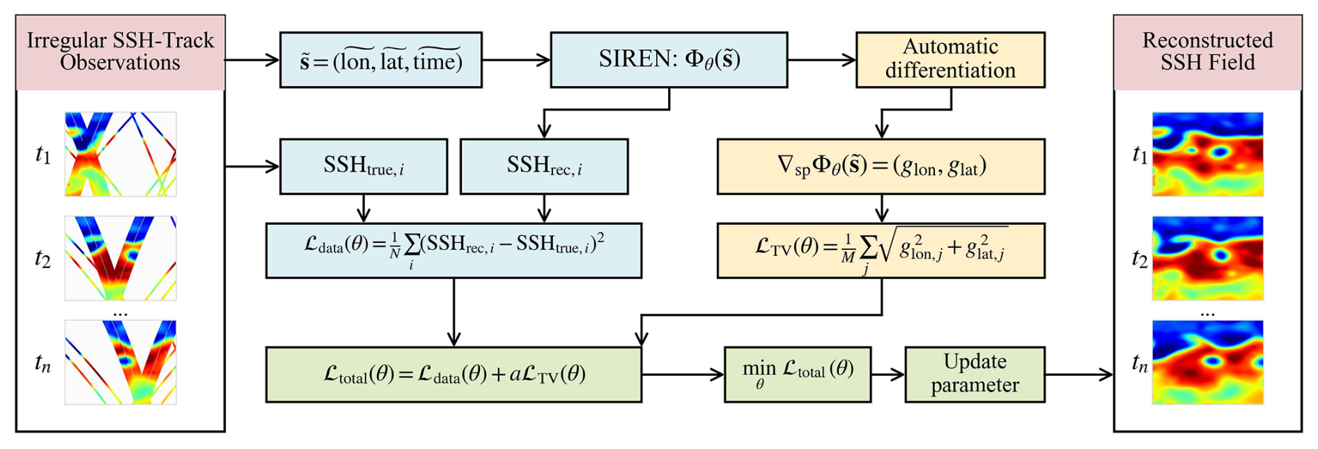
Figure 1 Architecture of the proposed INR-based SSH reconstruction framework, combining SIREN-based implicit representation with TV-based spatial-gradient regularization.

5 Experiment

This section evaluates the proposed INR-based SSH reconstruction framework in two benchmark settings. The OSE uses real satellite altimetry observations and tests the method under realistic sampling and measurement conditions. The OSSE uses simulated observations sampled from a numerical model, for which the complete SSH field is available as a reference. The experimental configurations, study domains, datasets, and evaluation protocols are described below.

5.1 Experimental configurations and evaluation protocols

The experiments are conducted in two study domains: the Western Mediterranean Sea (MEDIT) and the Gulf Stream region (GF), as shown in Fig. 2. The two domains correspond to different Ocean Data Challenges benchmarks: the SSH MapMed OSE benchmark for real observations (Ocean Data Challenges, 2023) and the NATL60 OSSE benchmark for controlled evaluation with a known reference field (Ocean Data Challenges, 2020). The datasets used here have been archived at Zenodo to ensure accessibility and reproducibility (Li, 2025a), and the experiments were implemented using the publicly available code (Li, 2025b).

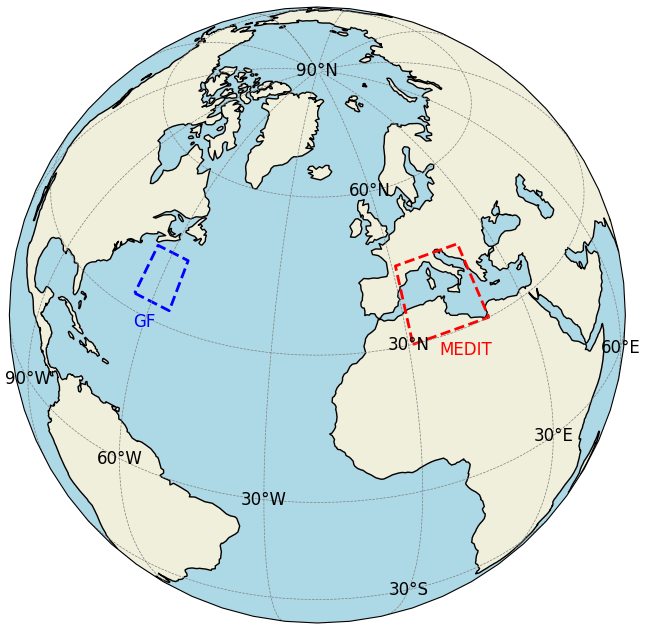
Figure 2 Geographical domains used in the experiments: Western Mediterranean (MEDIT) and Gulf Stream (GF) regions.

5.2 Evaluation indexes

To quantitatively assess reconstruction performance, we use two normalized skill-score diagnostics: an RMSE skill score for pointwise reconstruction accuracy and a PSD skill score for scale-dependent spectral consistency. The RMSE itself is first defined because it enters the normalized RMSE skill score.

(1) RMSE skill score

The RMSE between reconstructed and true SSH is first computed as

$$\begin{array}{}\text{(10)}& \text{RMSE}=\sqrt{\begin{array}{l}\frac{\mathrm{1}}{N}{\displaystyle }\sum _{i=\mathrm{1}}^N\left[{\text{SSH}}_{\text{rec}}({\text{lon}}_i,{\text{lat}}_i,{\text{time}}_i)\right.\\ {\left.-{\text{SSH}}_{\text{true}}({\text{lon}}_i,{\text{lat}}_i,{\text{time}}_i)\right]}^{\mathrm{2}}\end{array}},\end{array}$$

where N denotes the number of evaluation points. ${\text{SSH}}_{\text{rec}}({\text{lon}}_i,{\text{lat}}_i,{\text{time}}_i)$ is the reconstructed SSH at the ith spatio-temporal location, and ${\text{SSH}}_{\text{true}}({\text{lon}}_i,{\text{lat}}_i,{\text{time}}_i)$ is the corresponding reference SSH value.

Following the common definition of a skill score, this RMSE is normalized by the root-mean-square amplitude of the reference SSH field:

$$\begin{array}{}\text{(11)}& {\text{RMSE}}_{\text{SS}}=\mathrm{1}-{\displaystyle \frac{\text{RMSE}}{\text{RMS}\left({\text{SSH}}_{\text{true}}\right)}},\end{array}$$

where RMS(⋅) denotes the root-mean-square of the reference SSH field. A score of 1 corresponds to a perfect reconstruction, while larger values indicate better reconstruction skill.

This score is used with different averaging domains in the two experiments. In the OSE case, where the final test uses withheld along-track observations, we compute daily values RMSE_SS(t_k) and report their temporal mean over the valid evaluation days. In the OSSE case, where the complete NATL60 reference field is available, the same RMSE_SS definition is applied once to all valid grid points and evaluation times. Thus, in the OSSE comparison table, one RMSE_SS value is computed over these valid space–time evaluation points, rather than as a temporal mean of daily scores, a raw RMSE in metres, or a separate metric; it is rounded to two decimal places.

(2) Wavenumber–frequency PSD skill score

For the OSSE, where the complete NATL60 reference field is available, we assess the scale-dependent consistency of the reconstructed SSH fields using a power spectral density skill score in the wavenumber–frequency domain. To make the notation explicit, we write the PSD as a function of spatial wavenumber k and temporal frequency f. The wavenumber–frequency PSD skill score is defined as

$$\begin{array}{}\text{(12)}& {\text{PSD}}_{\text{SS}}(k,f)=\mathrm{1}-{\displaystyle \frac{\text{PSD}\left[{\text{SSH}}_{\text{rec}}-{\text{SSH}}_{\text{true}}\right](k,f)}{\text{PSD}\left[{\text{SSH}}_{\text{true}}\right](k,f)}}.\end{array}$$

Here, $\text{PSD}\left[\cdot \right](k,f)$ denotes the wavenumber–frequency power spectral density of a given field evaluated at spatial wavenumber k and temporal frequency f. The numerator represents the spectral energy of the reconstruction error, and the denominator represents the spectral energy of the reference SSH field. This score therefore measures the relative reconstruction skill at each wavenumber–frequency bin. A value close to 1 indicates that the reconstruction error is small relative to the reference signal at the corresponding spatio-temporal scale, whereas a value close to 0 indicates that the error energy is comparable to the signal energy.

Following the Ocean Data Challenges protocol, two PSD-score-based effective-scale diagnostics, λ_x and λ_t, are derived from the 0.5 contour of the normalized wavenumber–frequency PSD skill score PSD_SS(k,f). This threshold is used to summarize the shortest spatial and temporal scales that satisfy the adopted spectral-skill criterion. Specifically, λ_x is defined as the shortest spatial wavelength along this contour, while λ_t is defined as the shortest temporal period along the same contour. Smaller values of λ_x and λ_t indicate shorter effective scales under this diagnostic.

These quantities should be interpreted as threshold-based effective-scale diagnostics, rather than as nominal grid spacings or direct observational resolutions. In particular, when λ_x approaches the smallest wavelength represented by the evaluation grid and spectral discretization, it indicates that the adopted spectral-score criterion remains satisfied down to the smallest scales accessible in the diagnostic, rather than guaranteeing that all physical SSH structures at that scale are fully resolved.

5.3 Implementation details

The proposed INR-based reconstruction framework was implemented in PyTorch using a fully connected SIREN network with three hidden layers and 256 units per layer. The network takes normalized space–time coordinates as input and outputs the reconstructed SSH value. During training, the data-fidelity loss is evaluated at the available along-track observation points, while the spatial-gradient regularization term is evaluated over the reconstruction domain using automatic differentiation. The same implementation strategy is used for the OSE and OSSE experiments, with experiment-specific hyperparameters fixed across repeated runs. The detailed frequency factors, optimization settings, regularization coefficients, and run configuration are provided in the accompanying code.

5.4 Observed SSH experiment

This experiment aims to evaluate the capability of the proposed method to reconstruct sequences of SSH maps from incomplete real-world satellite altimetry measurements. All observations used in this section originate from operational nadir altimeters and correspond to actual SSH acquisitions.

5.4.1 Data preparation

The OSE configuration is conducted over the Western Mediterranean Sea within the domain $[\mathrm{1}\mathit{°}\mathrm{E},\mathrm{20}\mathit{°}\mathrm{E}]\times [\mathrm{30}\mathit{°}\mathrm{N},\mathrm{45}\mathit{°}\mathrm{N}]$. It assesses the reconstruction method under realistic satellite sampling and measurement conditions. This domain defines a common reconstruction target. Following the SSH MapMed OSE benchmark (Ocean Data Challenges, 2023), the reconstruction model is fitted using real along-track SSH observations from SARAL/Altika (alg), Haiyang-2B (h2b), Jason-3 (j3), Sentinel-3A (s3a), and Sentinel-3B (s3b) from 1 January–15 March 2021. The benchmark evaluation uses CryoSat-2 new-orbit observations (c2n) from 15 January–15 March 2021. The same non-CryoSat-2 input missions from 16–31 March 2021 and the corresponding CryoSat-2 observations form the validation dataset for hyperparameter selection.

5.4.2 Evaluation protocol and baseline methods

Two classes of comparative experiments are conducted to assess reconstruction performance.

(1) Comparison with optimal interpolation (OI)

We first compare our approach with the optimal interpolation (OI), which serves as the present-day standard for DUACS products provided by AVISO. This detailed comparison is conducted from multiple perspectives, including the orbital distribution of absolute errors, the spatial distribution of residuals on the grid, the temporal evolution of the RMSE skill score, and the spectral performance assessed via PSD.

(2) Comparison with state-of-the-art methods

Second, to further validate the robustness and general applicability of our approach, we compare it with several representative state-of-the-art methods, namely the Covariance-based optimal interpolation (BASELINE OI), the back-and-forth nudging algorithm combined with a quasigeostrophic model (BFN_QG) (Le Guillou et al., 2023), BFN_QG with Dirichlet boundary conditions (BFN_QG with coasts), and Wavevar (Ubelmann et al., 2021).

5.4.3 Detailed comparison with optimal interpolation

(1) Error distribution and spatial RMSE

Figure 3 provides a combined error diagnostic for the INR-based reconstruction and the OI baseline. Figure 3a shows the cumulative distribution function (CDF) of signed SSH residuals at the withheld along-track observation locations. The residual is defined as SSH_rec−SSH_obs, so positive values indicate overestimation and negative values indicate underestimation relative to the withheld observations. Compared with OI, the INR residuals are more tightly concentrated around zero, indicating a smaller residual spread and little systematic offset. The mean residual, standard deviation, and RMSE are 0.000, 0.026, and 0.026 m for INR, respectively, compared with 0.004, 0.039, and 0.039 m for OI. This result suggests that INR is more consistent with the withheld along-track observations than OI.

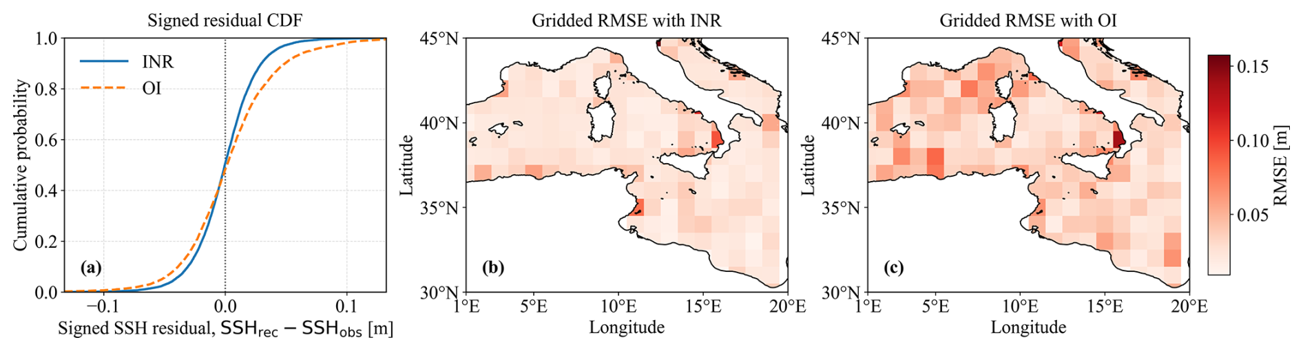
Figure 3 Combined error diagnostics for the INR-based reconstruction and OI. (a) Cumulative distribution function (CDF) of signed SSH residuals, defined as SSH_rec−SSH_obs, at withheld along-track observation locations. (b, c) Gridded RMSE maps for INR and OI, respectively, computed from withheld residuals within each spatial grid cell. Coastlines are shown in panels (b, c).

Figure 3b and c show gridded RMSE maps for the INR-based reconstruction and OI, respectively. The maps are obtained by assigning the withheld along-track residuals to spatial grid cells and computing the RMSE within each cell using Eq. (10), with the withheld observations used as the reference values. These RMSE maps complement the residual CDF by showing where the remaining errors are located. Overall, the INR-based reconstruction exhibits lower RMSE values than OI over much of the domain. Some localized high-RMSE regions remain for both methods, especially near parts of the domain boundary and coastal areas, but they are weaker and less extensive in the INR map.

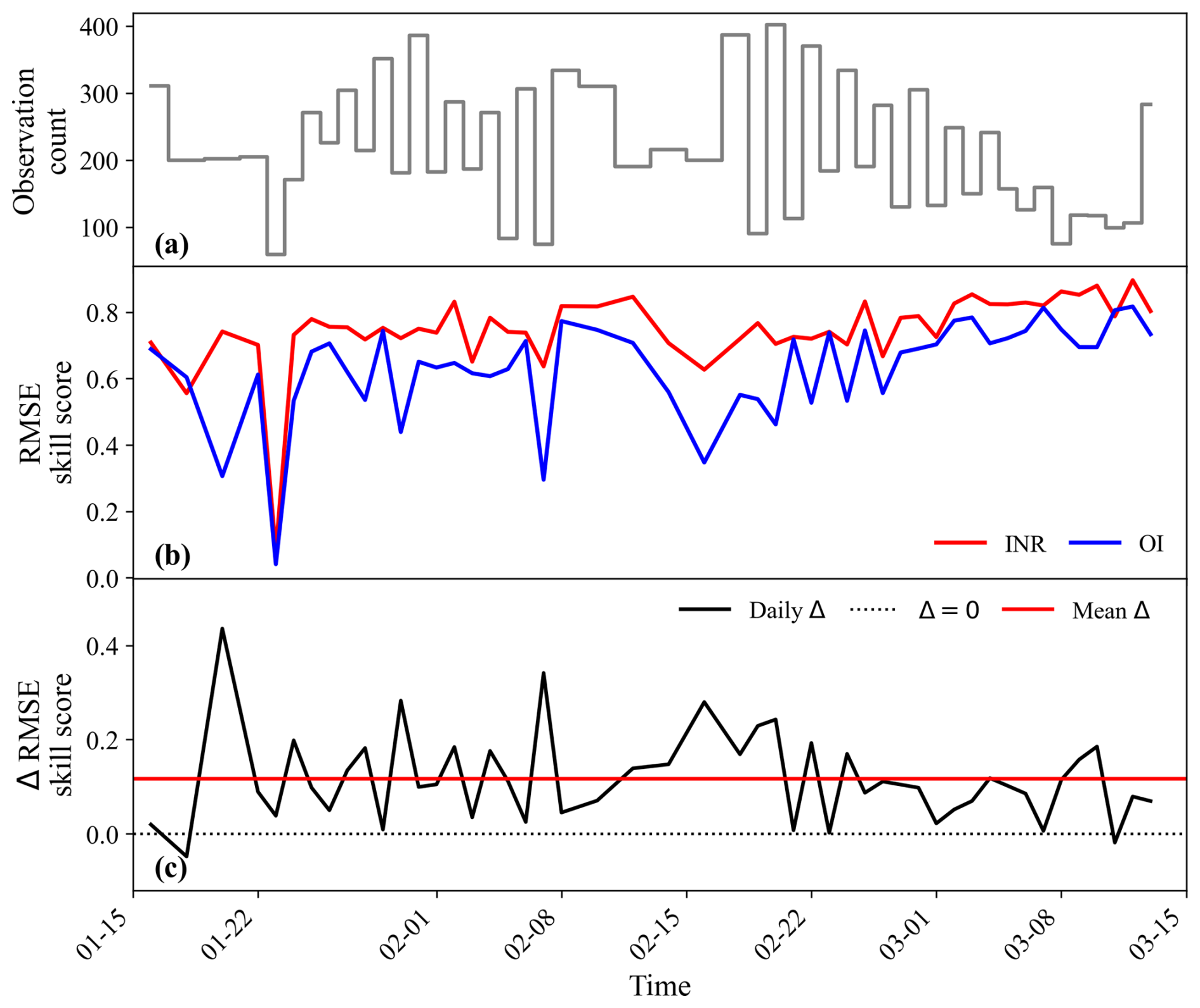
Figure 4 Temporal variability of the reconstruction skill. (a) Daily number of available along-track observations used for the evaluation. (b) Daily RMSE skill scores for the INR-based reconstruction and OI. (c) Daily paired difference in RMSE skill score, $\mathrm{\Delta }={\text{RMSE}}_{\text{SS}}^{\text{INR}}-{\text{RMSE}}_{\text{SS}}^{\text{OI}}$; the dotted line denotes Δ=0, and the red line denotes the mean difference. Only valid paired evaluation days are shown.

(2) Temporal performance: RMSE skill score

The temporal behaviour of the reconstruction is assessed using the RMSE skill score, denoted as RMSE_SS and computed according to Eq. (11). Figure 4 summarizes the temporal variability of the evaluation data and the corresponding reconstruction skill. Figure 4a shows the daily number of available along-track observations used for the evaluation. The observation count varies noticeably over time, reflecting the non-uniform temporal sampling of the along-track data.

Figure 4b shows the daily RMSE skill scores for the INR-based reconstruction and OI. The INR method yields higher RMSE_SS values than OI over most valid paired evaluation days. Across 49 paired evaluation days, the mean daily RMSE_SS is 0.748 for INR and 0.631 for OI, with standard deviations of 0.120 and 0.151, respectively. This indicates that INR improves the average daily test skill and also shows a slightly smaller day-to-day spread than OI.

Figure 4c further reports the paired daily difference between INR and OI. We define this difference as $\mathrm{\Delta }={\text{RMSE}}_{\text{SS}}^{\text{INR}}-{\text{RMSE}}_{\text{SS}}^{\text{OI}}$. Positive values indicate days when INR outperforms OI. The paired daily difference is 0.117±0.095, with an approximate 95 % confidence interval of [0.090,0.143], and INR outperforms OI on 95.9 % of the evaluated days. The positive confidence interval and the large fraction of positive daily differences indicate that the INR improvement is not driven by a few isolated dates, but is maintained over most of the OSE evaluation period. The remaining day-to-day variability indicates that the improvement is not identical on every date. Some dates are more difficult because the withheld tracks provide fewer samples or sample more challenging parts of the domain.

(3) Spectral diagnostics and effective scale

Spectral diagnostics for the OSE are presented in Fig. 5. Because the withheld CryoSat-2 reference is available only on sparse along-track segments, these diagnostics are one-dimensional along-track spatial spectra rather than the wavenumber–frequency diagnostic of Eq. (12). Figure 5a shows the one-dimensional along-track spatial PSDs of the INR reconstruction, the withheld CryoSat-2 reference SSH, and the OI baseline. Following the publicly available SSH MapMed OSE benchmark evaluation procedure (Ocean Data Challenges, 2023), the reconstruction is sampled at the CryoSat-2 locations and times. Continuous CryoSat-2 tracks are separated at time gaps greater than 4 s and partitioned into nominal 300 km segments with 50 % overlap; Welch spectra are computed from the pooled valid segments. Figure 5b shows the corresponding along-track PSD skill score, where PSD_err is the one-dimensional spatial PSD of the reconstruction error and PSD_ref is the one-dimensional spatial PSD of the CryoSat-2 reference SSH on these same segments. The 0.5 crossing is used to derive the PSD-score-based effective spatial scale. Under this diagnostic, INR reaches an effective spatial scale of 106 km, whereas OI reaches 154 km. This indicates that, along the withheld CryoSat-2 tracks, the INR reconstruction remains spectrally closer to the reference than OI over a broader range of spatial wavelengths, including shorter wavelengths under the adopted PSD-score criterion.

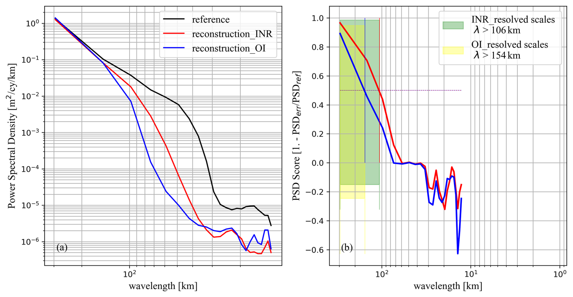
Figure 5 OSE along-track spectral diagnostics. (a) One-dimensional along-track spatial PSDs of the INR reconstruction, withheld CryoSat-2 reference SSH, and OI baseline. (b) Corresponding PSD skill score, $\mathrm{1}-{\text{PSD}}_{\text{err}}/{\text{PSD}}_{\text{ref}}$, with the 0.5 crossing used to derive the PSD-score-based effective spatial scale. Here, PSD_err and PSD_ref are the one-dimensional spatial PSDs of the reconstruction error and CryoSat-2 reference SSH, respectively, computed from the valid CryoSat-2 along-track segments following the SSH MapMed OSE benchmark evaluation procedure (Ocean Data Challenges, 2023). Higher scores indicate smaller relative spectral errors.

5.4.4 Comprehensive comparison with multiple methods

This section provides a broader evaluation of the proposed approach by comparing it against several representative reconstruction methods. The assessment relies on the two quantitative metrics introduced in Sect. 5.2, namely the temporal mean of the RMSE skill score, denoted as $\stackrel{\mathrm{‾}}{{\text{RMSE}}_{\text{SS}}}$, and the PSD-score-based effective spatial scale λ_x. Here, $\stackrel{\mathrm{‾}}{{\text{RMSE}}_{\text{SS}}}$ is defined as

$$\begin{array}{}\text{(13)}& \stackrel{\mathrm{‾}}{{\text{RMSE}}_{\text{SS}}}={\displaystyle \frac{\mathrm{1}}{N_{\text{day}}}}\sum _{k=\mathrm{1}}^{N_{\text{day}}}{\text{RMSE}}_{\text{SS}}\left(t_k\right),\end{array}$$

where N_day denotes the number of valid evaluation days, and RMSE_SS(t_k) denotes the RMSE skill score computed from Eq. (11) on the kth valid evaluation day. The results are summarized in Table 1.

Table 1 Results of different methods using satellite altimetry observations in the Mediterranean region. $\stackrel{\mathrm{‾}}{{\text{RMSE}}_{\text{SS}}}$ denotes the temporal mean of the RMSE skill score over the valid evaluation days. Bold values denote best performance.

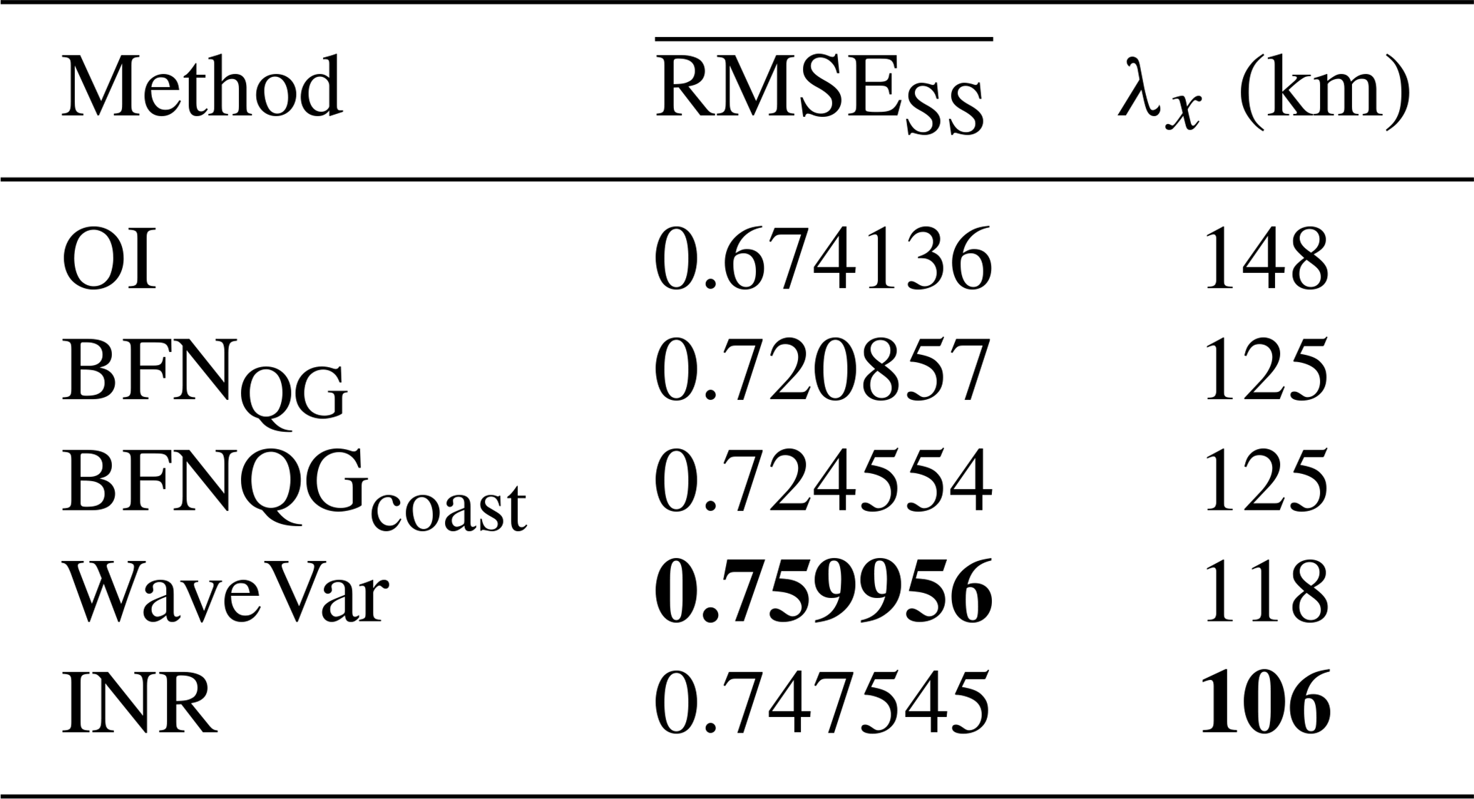
As shown in Table 1, INR achieves a slightly lower $\stackrel{\mathrm{‾}}{{\text{RMSE}}_{\text{SS}}}$ than WaveVar, but it gives the smallest λ_x among all compared methods. This indicates that INR does not provide the best temporal-mean global error score in this comparison, but shows a more favorable PSD-score-based spatial effective-scale diagnostic under the adopted PSD-skill criterion. This behavior is consistent with the characteristics of the proposed framework. The SIREN-based representation describes SSH as a continuous function of spatial and temporal coordinates, while the gradient-based regularization constrains unstable or noisy variations in the learned field. Together, these two components help maintain competitive overall reconstruction accuracy while improving the spectral consistency and spatial coherence of the reconstructed SSH field.

5.5 Simulated SSH experiment

This section evaluates the proposed method using simulated SSH data. Unlike real altimetric observations, the model generates complete reference SSH fields, enabling detailed quantitative assessment of interpolation accuracy and effective spatio-temporal resolution.

5.5.1 Data preparation

The OSSE configuration is conducted over a dynamically active portion of the Gulf Stream region, spanning 65–55° W and 33–43° N. It uses the NATL60 SSH simulation, based on the Nucleus for European Modelling of the Ocean (NEMO) (Ajayi et al., 2020), as the known reference field. This domain defines a common reconstruction target. Following the NATL60 OSSE benchmark (Ocean Data Challenges, 2020), the reconstruction model is fitted using pseudo-altimetric observations from the four-nadir-plus-SWOT configuration during the assessment period from 22 October–2 December 2012. The complete NATL60 SSH simulation over the same domain and period provides the reference for full-domain evaluation. Pseudo-altimetric observations from the four-nadir-plus-SWOT configuration and the corresponding NATL60 SSH fields from 2 January–30 September 2013 are used as the validation dataset for hyperparameter selection.

5.5.2 Evaluation protocol and baseline methods

The experimental setup aims to comprehensively evaluate the proposed approach's performance and robustness. First, we compare the reconstructed SSH with the model-simulated SSH reference using both direct SSH errors and spatial-gradient diagnostics. The gradient diagnostics are used to examine whether the reconstructed field captures major spatial transitions, such as fronts and eddy boundaries. Second, to further validate the general applicability of our method, we compare it with several existing state-of-the-art interpolation and reconstruction methods, including DUACS (a traditional covariance-based optimal interpolation method, Taburet et al., 2019), three model-based data assimilation schemes: BFN (a data assimilation method that follows quasi-geostrophic dynamics, Le Guillou et al., 2021), DYMOST (dynamic OI accounting for the SSH nonlinear temporal propagation, Ubelmann et al., 2016), and MIOST (multiscale OI, Ubelmann et al., 2021). Finally, we compare with the supervised 4DVarNet method (based on a neural network architecture backed by a variational formulation, Beauchamp et al., 2023). Performance is assessed using the statistical metrics defined in Sect. 5.2, including the mean RMSE skill score $\stackrel{\mathrm{‾}}{{\text{RMSE}}_{\text{SS}}}$ and the spectral diagnostics λ_x and λ_t. These metrics summarize reconstruction accuracy and the PSD-score-based effective spatial and temporal scales under the Ocean Data Challenges benchmark protocol.

5.5.3 Evaluation of reconstructed sea surface height

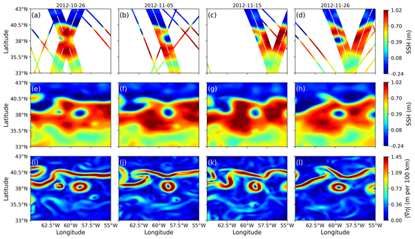
Figure 6 shows qualitative examples at four selected times covering the evaluation period. Specifically, we divide the evaluation period into four approximately equal sub-periods and use the middle valid snapshot from each sub-period. The four columns compare the along-track observations, the reconstructed SSH fields, and the corresponding physical SSH-gradient magnitudes.

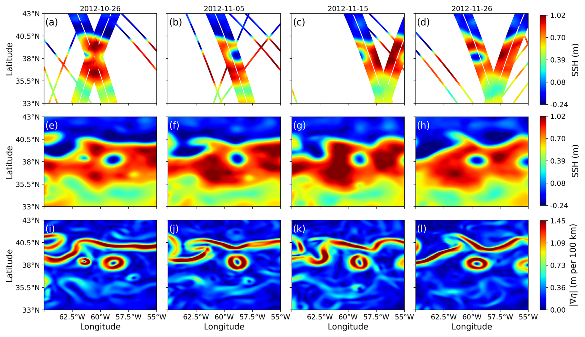
Figure 6 Qualitative OSSE snapshots of SSH reconstruction from sparse satellite-like observations. The four columns show selected dates from four approximately equal sub-periods of the evaluation period. Rows show sparse nadir/SWOT-like pseudo-observations, reconstructed SSH, and the physical SSH-gradient magnitude derived from the differentiable SIREN field. SSH is in metres, $\left|\mathrm{\nabla }\mathit{\eta }\right|$ is in metres per 100 km, and the full temporal evolution is provided in Supplementary Video S1 (https://zenodo.org/records/21231911).

The physical SSH-gradient magnitude shown in the bottom row is a visualization diagnostic distinct from the normalized-coordinate gradients used in the TV regularization. It is derived from automatic differentiation of the SIREN representation and explicitly rescaled to physical distance. This diagnostic uses one of the key properties of the INR framework, namely that the reconstructed SSH field is represented as a continuous and differentiable function of the spatio-temporal coordinates. Let $\mathit{\eta }(\text{lon},\text{lat},t)={\mathrm{\Phi }}_{\mathit{\theta }}\left(\stackrel{\mathrm{̃}}{\mathit{s}}\right)$ denote the reconstructed SSH field, where $\stackrel{\mathrm{̃}}{\mathit{s}}=(\stackrel{\mathrm{̃}}{\text{lon}},\stackrel{\mathrm{̃}}{\text{lat}},\stackrel{\mathrm{̃}}{\text{time}})$ is the normalized spatio-temporal coordinate, and lon and lat denote longitude and latitude in radians. Automatic differentiation first gives the derivatives of Φ_θ with respect to the normalized input coordinates. These normalized-coordinate derivatives are then rescaled to derivatives with respect to longitude and latitude:

$$\begin{array}{}\text{(14)}& {\displaystyle \frac{\partial \mathit{\eta }}{\partial \text{lon}}}={\displaystyle \frac{\partial {\mathrm{\Phi }}_{\mathit{\theta }}}{\partial \stackrel{\mathrm{̃}}{\text{lon}}}}{\displaystyle \frac{\partial \stackrel{\mathrm{̃}}{\text{lon}}}{\partial \text{lon}}},{\displaystyle \frac{\partial \mathit{\eta }}{\partial \text{lat}}}={\displaystyle \frac{\partial {\mathrm{\Phi }}_{\mathit{\theta }}}{\partial \stackrel{\mathrm{̃}}{\text{lat}}}}{\displaystyle \frac{\partial \stackrel{\mathrm{̃}}{\text{lat}}}{\partial \text{lat}}}.\end{array}$$

These longitude and latitude derivatives are then converted into physical-distance derivatives using the Earth-radius scale factors:

$$\begin{array}{}\text{(15)}& {\displaystyle \frac{\partial \mathit{\eta }}{\partial x}}={\displaystyle \frac{\mathrm{1}}{R\cos \left(\text{lat}\right)}}{\displaystyle \frac{\partial \mathit{\eta }}{\partial \text{lon}}},{\displaystyle \frac{\partial \mathit{\eta }}{\partial y}}={\displaystyle \frac{\mathrm{1}}{R}}{\displaystyle \frac{\partial \mathit{\eta }}{\partial \text{lat}}},\end{array}$$

where R is the Earth radius. The physical SSH-gradient magnitude is defined as

$$\begin{array}{}\text{(16)}& \left|\mathrm{\nabla }\mathit{\eta }\right|={\left[{\left({\displaystyle \frac{\partial \mathit{\eta }}{\partial x}}\right)}^{\mathrm{2}}+{\left({\displaystyle \frac{\partial \mathit{\eta }}{\partial y}}\right)}^{\mathrm{2}}\right]}^{\mathrm{1}/\mathrm{2}}.\end{array}$$

For visualization, we plot ${\mathrm{10}}^{\mathrm{5}}\left|\mathrm{\nabla }\mathit{\eta }\right|$, corresponding to units of m per 100 km. Therefore, the bottom-row panels should be interpreted as physical SSH-gradient magnitudes derived from the differentiable SSH representation, rather than as direct velocity or vorticity fields. Their further conversion into geostrophic velocity would require additional dynamical assumptions.

The reconstructed SSH fields in the middle row reproduce the main mesoscale SSH patterns across the four snapshots, including eddy-like structures and their surrounding transition regions. The corresponding gradient-magnitude maps in the bottom row emphasize regions where the reconstructed SSH field changes rapidly, such as eddy peripheries and frontal-like transition zones. These high-gradient regions are spatially consistent with the structures visible in the reconstructed SSH fields, indicating that the learned field preserves coherent spatial variations rather than producing isolated noisy gradients.

The gradient diagnostic provides a complementary view of the reconstructed SSH field by showing whether rapid spatial transitions, such as fronts and eddy boundaries, are represented as coherent structures.

While Fig. 6 shows four selected snapshots, the full temporal evolution of the along-track observations, reconstructed SSH fields, and corresponding physical SSH-gradient magnitudes is provided in Video Supplement S1. Together with the snapshot examples, the video provides a more complete visual assessment of the reconstruction behavior over the evaluation period.

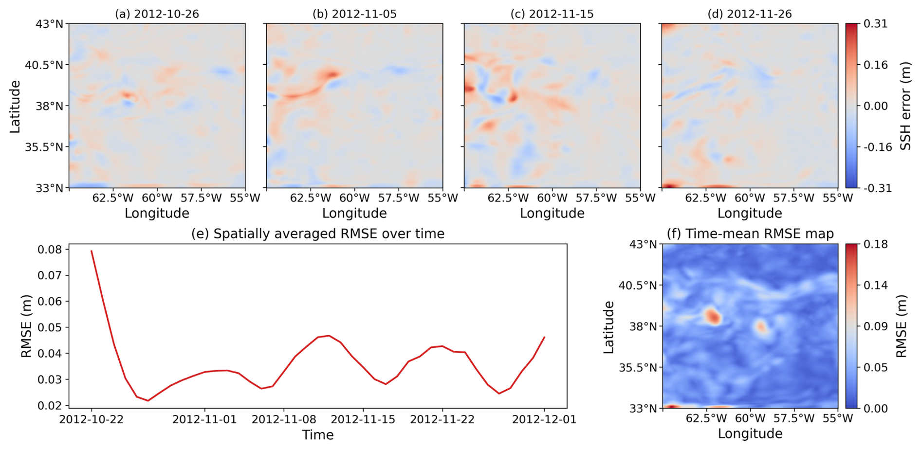
Figure 7 Spatio-temporal reconstruction error of the proposed method in the OSSE experiment. Panels (a–d) show the instantaneous error field e at the same four representative dates as in the preceding qualitative INR reconstruction figure. Panel (e) shows RMSE_space(t_j) , and panel (f) shows RMSE_time(x_m,y_n) , as defined in Eq. (17). All errors are computed in the original SSH physical space, with units of metres.

5.5.4 Spatio-temporal reconstruction error

Since the OSSE configuration provides the complete NATL60 SSH field as the reference, the full spatio-temporal reconstruction error can be directly evaluated. The error field and the two RMSE summaries used below are defined together as

$$\begin{array}{}\text{(17)}& \begin{array}{rl}{\displaystyle }& {\displaystyle }e(x_m,y_n,t_j)={\text{SSH}}_{\text{rec}}(x_m,y_n,t_j)-{\text{SSH}}_{\text{true}}(x_m,y_n,t_j),\\ {\displaystyle }& {\displaystyle }{\text{RMSE}}_{\text{space}}\left(t_j\right)={\left[{\displaystyle \frac{\mathrm{1}}{N_x{N}_y}}\sum _{m=\mathrm{1}}^{N_x}\sum _{n=\mathrm{1}}^{N_y}e(x_m,y_n,t_j{)}^{\mathrm{2}}\right]}^{\mathrm{1}/\mathrm{2}},\\ {\displaystyle }& {\displaystyle }{\text{RMSE}}_{\text{time}}(x_m,y_n)={\left[{\displaystyle \frac{\mathrm{1}}{N_t}}\sum _{j=\mathrm{1}}^{N_t}e(x_m,y_n,t_j{)}^{\mathrm{2}}\right]}^{\mathrm{1}/\mathrm{2}}.\end{array}\end{array}$$

Here, SSH_rec denotes the reconstructed SSH field and SSH_true denotes the NATL60 reference field. All errors in this analysis are computed in the original SSH physical space, with units of metres.

Figure 7 presents the spatio-temporal reconstruction error of the proposed method in the OSSE experiment. Figure 7a–d show the instantaneous SSH reconstruction error at the same four selected dates as those used in the preceding INR reconstruction figure. These dates were obtained by dividing the evaluation period into four approximately equal sub-periods and selecting the middle valid snapshot from each sub-period. The instantaneous error maps show that errors are relatively small over much of the domain. Larger errors are mainly localized in dynamically active regions with stronger SSH variability and sharper gradients. This indicates that energetic mesoscale structures remain more challenging to reconstruct accurately under sparse satellite-like sampling.

Figure 7e shows the spatially averaged RMSE over time. This time series summarizes how the domain-mean reconstruction error varies among the evaluated time slices. The RMSE is relatively larger near the beginning and then fluctuates during the evaluation period. Larger RMSE values indicate time slices in which the SSH structures and sampling constraints are more challenging for the reconstruction.

To summarize the spatial distribution of the reconstruction error over the full evaluation period, Fig. 7f shows the time-mean RMSE map. The time-mean RMSE remains low over most of the domain, while several localized regions exhibit relatively larger values. These localized high-error regions are mainly associated with areas where the SSH field has stronger spatial variability and sharper gradients. This result further shows that the proposed method can reconstruct the broad SSH pattern and maintain spatial coherence over most of the domain, while dynamically active mesoscale structures remain more difficult to reproduce accurately.

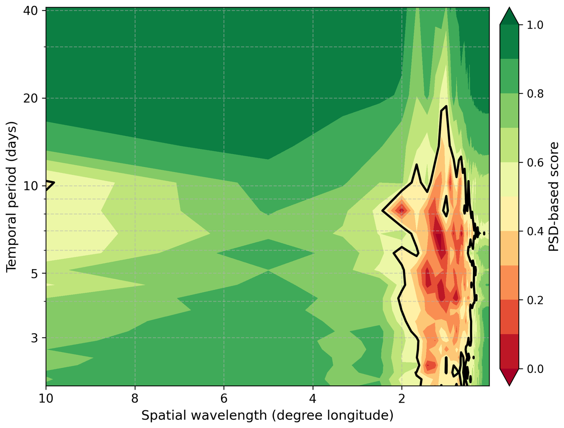
Figure 8 PSD-based skill score of the INR reconstruction in the wavelength–period domain. The black contour denotes the 0.5 level used to derive the PSD-score-based effective-scale diagnostics following the Ocean Data Challenges protocol. The spatial value λ_x=0.03° is the shortest wavelength reached by this contour. The temporal contour reaches the 2.05 d lower boundary imposed by the daily-sampled PSD calculation, representing the best temporal value accessible under the common comparison; it does not demonstrate skill at shorter periods or an exact temporal resolved scale.

5.5.5 Comparison of multiple methods for SSH reconstruction

Table 2 reports the performance of the proposed INR method in comparison with several representative state-of-the-art approaches. Unless otherwise specified, INR denotes the full proposed model with TV regularization, while “INR without TV” is used only as an ablation variant. In terms of the OSSE RMSE_SS computed over all valid grid points and evaluation times, INR performs on par with the top-performing schemes. Although its RMSE_SS value is slightly lower than that of 4DVarNet v2022, INR attains the smallest diagnosed spatial scale λ_x under the adopted Ocean Data Challenges PSD-score protocol. Both INR configurations also reach the 2.05 d lower boundary of the common daily-sampled temporal diagnostic, whereas the non-INR methods cross the 0.5 threshold at longer periods. This boundary-limited result establishes the relative advantage of INR within the common benchmark, but it does not rank performance at periods shorter than 2.05 d.

The effect of the TV regularization term is isolated by comparing the full INR model with an ablation variant in which the TV term is removed while all other settings are kept unchanged. The ablation result shows that removing the TV term has little influence on the normalized RMSE score, which remains approximately 0.94. Both configurations reach the 2.05 d lower boundary of the temporal diagnostic, so this boundary-limited value cannot be used to distinguish their sub-2.05 d performance. In contrast, the diagnosed spatial scale λ_x, derived from the 0.5 contour of the PSD-score field, changes from 0.12° without TV regularization to 0.03° with TV regularization. This indicates that the TV term mainly affects the spatial PSD-score diagnostic, by reducing isolated large gradients and part of the high-wavenumber error energy, while the domain-averaged pointwise error changes little.

Table 2 Performance comparison of SSH reconstruction methods on the simulated altimetry dataset in the Gulf Stream domain. Here, RMSE_SS is the normalized RMSE skill score defined in Eq. (11), computed once over all valid grid points and evaluation times in the OSSE experiment. Unless otherwise specified, INR denotes the full proposed model with TV regularization, while “INR without TV” denotes the ablation variant used to assess the effect of the TV term. Bold values denote the best performance for each metric. Entries marked ^* reach the temporal Nyquist boundary of the daily-sampled diagnostic (2.05 d), which is the best value accessible under this common comparison; performance at shorter temporal periods is not assessed.

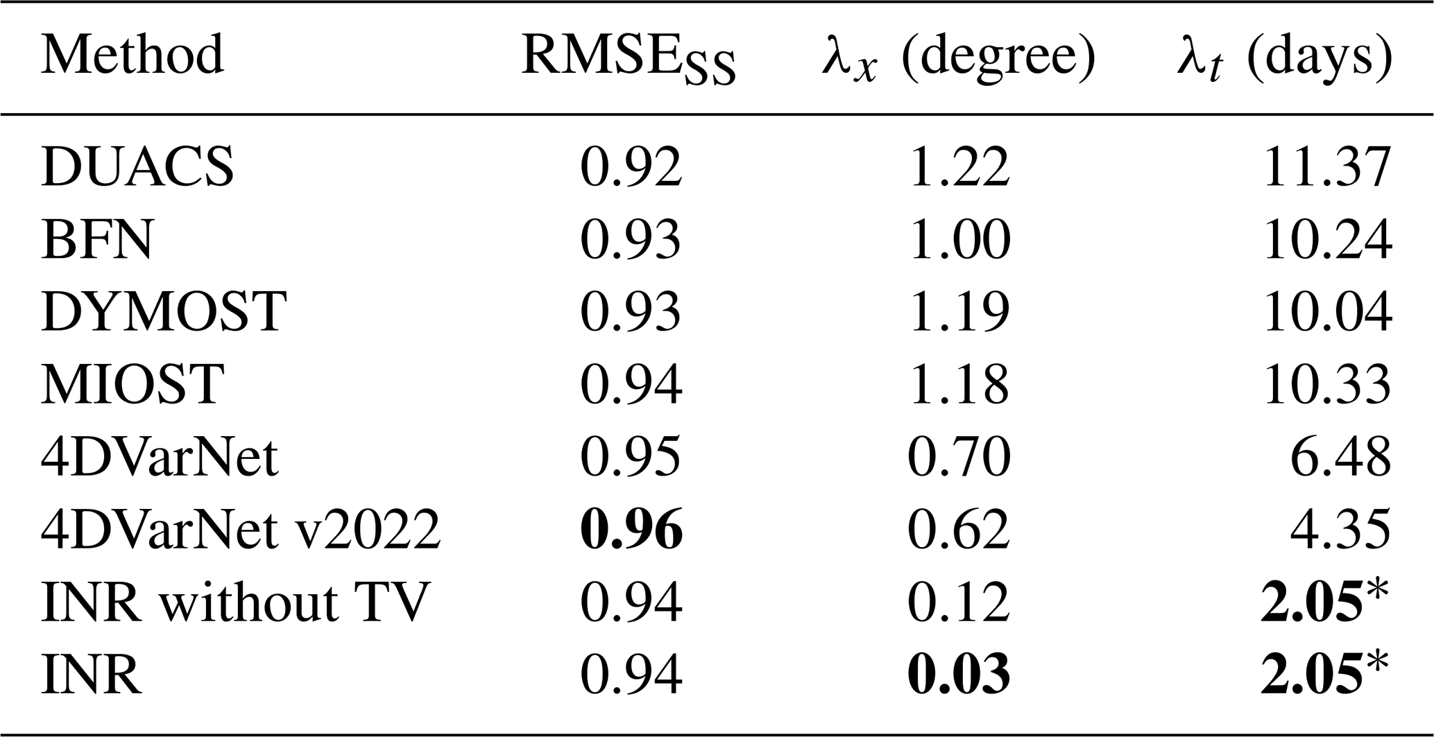
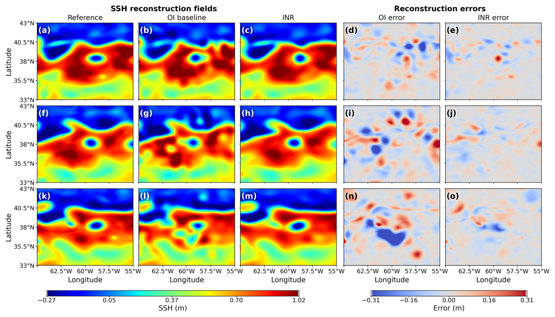
Figure 9 Qualitative comparison between the OI baseline and INR under the four-nadir observation setting. From top to bottom, the rows correspond to three representative evaluation times selected according to the 0.1, 0.5, and 0.9 quantiles of the OI SSH reconstruction error, respectively. The first three columns show the NATL60 reference SSH field, the OI baseline reconstruction, and the INR reconstruction, respectively. The last two columns show the corresponding SSH reconstruction errors of the OI baseline and INR relative to the NATL60 reference.

As reported in Table 2, INR gives the smallest PSD-score-based effective spatial scale and reaches the lowest temporal value accessible under the common evaluation criterion. To clarify how these diagnostics are obtained and how they should be interpreted, Fig. 8 shows the PSD-based score in the wavelength–period domain. The score is generally high for long temporal periods, especially above approximately 15–20 d, over a broad range of spatial wavelengths, indicating that slowly varying SSH components are well reconstructed. Relatively high scores are also observed at broad spatial wavelengths, roughly larger than 3°, suggesting that large-scale SSH variability is captured with small relative spectral error. In contrast, the main low-score region is concentrated at shorter temporal periods and intermediate spatial wavelengths, approximately within 3–10 d and 0.5–2°. This indicates that rapidly evolving and spatially complex SSH variability remains more challenging to reconstruct.

The temporal axis terminates at 2.05 d because the PSD calculation uses 41 daily SSH fields. Its largest positive temporal frequency is therefore $\mathrm{20}/\mathrm{41}{\mathrm{d}}^{-\mathrm{1}}$, corresponding to a shortest represented temporal period of $\mathrm{41}/\mathrm{20}=\mathrm{2.05}\mathrm{d}$. The black 0.5 contour reaches this lower boundary. Thus, within the common benchmark, INR maintains the PSD-score criterion down to the highest temporal frequency accessible to the daily-sampled diagnostic, whereas the non-INR methods in Table 2 cross the criterion at longer periods. This is a valid relative comparison under the shared protocol. However, the boundary-limited 2.05 d value neither establishes skill at periods shorter than 2.05 d nor provides an exact temporal resolution. Some high-score colors adjacent to this boundary should likewise not be interpreted as sub-2.05 d skill. In addition, the PSD-based score is a relative spectral-error measure and can be sensitive where the reference spectral energy is weak. Following the Ocean Data Challenges protocol, the spatial scale λ_x=0.03° remains a contour-derived comparative diagnostic, rather than a nominal grid spacing or a guarantee that all SSH structures at this scale are fully resolved.

In addition to the quantitative comparison above, we provide a qualitative comparison with the benchmark OI baseline. The comparison is shown for the four-nadir setting, for which reproducible gridded OI outputs are provided by the benchmark. This allows the spatial reconstruction patterns, reconstruction errors, and derivative-based diagnostics of OI and INR to be compared on the same input observations and evaluation grid.

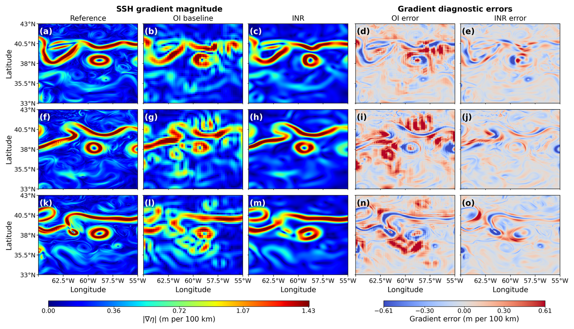
Figure 10 Derivative-based qualitative comparison between the OI baseline and INR under the four-nadir observation setting. From top to bottom, the rows correspond to three representative evaluation times selected according to the 0.1, 0.5, and 0.9 quantiles of the OI SSH reconstruction error, respectively. The first three columns show the SSH gradient magnitude $\left|\mathrm{\nabla }\mathit{\eta }\right|$ computed from the NATL60 reference field, the OI baseline reconstruction, and the INR reconstruction, respectively. The last two columns show the corresponding gradient diagnostic errors of the OI baseline and INR relative to the NATL60 reference.

Figure 9 compares the NATL60 reference SSH field, the OI baseline reconstruction, and the INR reconstruction at three representative evaluation times. The rows correspond to cases selected according to the 0.1, 0.5, and 0.9 quantiles of the OI SSH reconstruction error, respectively. Both methods reproduce the broad SSH distribution from sparse along-track observations, while noticeable differences appear in dynamically active regions with strong spatial variability. The error maps show that the largest residuals tend to occur near strong-gradient frontal and eddy-like features visible in the reference, indicating that these regions remain challenging under sparse observational constraints. Compared with the OI baseline, the INR error maps in these selected cases contain fewer broad high-amplitude residual patches and show a more spatially continuous SSH pattern. This qualitative comparison complements the quantitative metrics by showing where the main residual patterns occur in the selected OSSE examples.

To further examine the behavior of the reconstructed derivative fields, we compare the SSH gradient magnitude derived from the NATL60 reference field, the OI baseline reconstruction, and the INR reconstruction. This derivative-based diagnostic complements the SSH snapshot comparison by focusing on fronts, eddy boundaries, and other high-gradient regions. The same three evaluation times as in Fig. 9 are used for consistency.

Figure 10 shows the corresponding gradient-magnitude fields and gradient diagnostic errors. The OI-derived gradients are comparatively diffuse and show some small-scale artifacts in these examples, whereas the INR-derived gradients follow the main frontal and eddy-like bands more continuously. The diagnostic error maps also show that sharp fronts and eddy boundaries remain the main sources of gradient discrepancies for both methods, partly because small spatial displacements can lead to pronounced derivative errors. Some very narrow gradient filaments in the NATL60 reference are absent from both reconstructions, as expected under sparse satellite-like sampling. We therefore use this comparison mainly to assess the dominant gradient structures and the location of large gradient errors. Overall, the derivative-based comparison indicates that the gradient-regularized INR framework reduces some spurious derivative artifacts relative to the OI baseline while retaining the dominant gradient structures visible in the reference.

6 Discussion

The experiments use two complementary Ocean Data Challenges benchmarks: the NATL60-based OSSE framework (Ocean Data Challenges, 2020) and the SSH MapMed OSE framework (Ocean Data Challenges, 2023). The OSSE setting provides a complete reference field for controlled evaluation, whereas the OSE setting tests the method with real satellite altimetry observations and withheld along-track test data. Together, these experiments show that the proposed INR framework can provide competitive SSH reconstruction skill and spatially coherent derivative-based diagnostics under sparse sampling, while also revealing several practical limitations.

6.1 Methodological characteristics and relation to existing approaches

The proposed framework differs from conventional SSH mapping approaches mainly in how the field is represented. OI-based products estimate values on a predefined grid using prescribed covariance models, while model-based assimilation methods introduce explicit dynamical constraints. By contrast, the INR model learns SSH as a continuous function of spatial and temporal coordinates from the available observations. Once optimized for a target reconstruction problem, this function can be evaluated at requested coordinates within the reconstruction domain and period, and its differentiability supports gradient diagnostics. Compared with supervised deep-learning approaches such as 4DVarNet-type methods, it does not require a large set of paired sparse-observation and full-field training examples. Instead, its parameters are optimized from the available observations for the target reconstruction problem. This formulation is flexible, but it remains a reconstruction model constrained by observations and regularization, not a replacement for full dynamical data assimilation. OI and related analytical approaches remain useful because their assumptions are explicit and, in the case of OI, can provide uncertainty estimates associated with the prescribed covariance model. The optimized INR should therefore be viewed as a reconstruction constrained by the available observations over the prescribed reconstruction window. The length of this window describes the temporal coverage of the input observations, not a physical time scale learned by the network for the regional dynamics.

6.2 Applicability and limitations

The main limitation is that reconstruction quality remains constrained by the available observations. The INR learns SSH as a continuous function of spatial and temporal coordinates from sparse samples and can be queried at unobserved space–time points within the chosen reconstruction domain and time window. This interpolation capability should not be interpreted as unconstrained extrapolation: poorly sampled SSH structures or rapidly evolving events remain difficult to recover. The PSD-score-based effective scale should also be interpreted as a diagnostic of reconstruction skill under a given sampling and evaluation protocol, rather than as the nominal grid spacing of the output field or the NATL60 reference.

The balance between data fitting and regularization is another practical issue. The objective function should be understood as a regularized least-squares formulation rather than a full Bayesian model. The data-fidelity loss treats the along-track observations as having a common error variance, so the observed samples contribute equally in the current implementation. The TV term acts as a regularization preference on spatial gradients, and the coefficient a is a global hyperparameter rather than a local uncertainty- or region-dependent parameter. Strong regularization can improve spatial coherence but may smooth physically meaningful variability, whereas weak regularization can leave unstable gradients in sparsely observed areas. A more systematic strategy for choosing the regularization strength, and possible extensions using observation-dependent error variances, physically scaled spatial-gradient penalties, spatially varying regularization coefficients, or Bayesian uncertainty quantification, would be useful in future work.

The OSE and OSSE results should also be interpreted according to their different evaluation settings. The OSSE experiment allows full-field evaluation against NATL60, whereas the OSE experiment uses withheld-mission along-track test data because no complete true SSH field is available. The OSE statistics are therefore best read as reconstruction or mapping skill under the benchmark sampling configuration, not as a strict test of long-term temporal extrapolation. In the OSE case, some dynamical correlation may remain between training and validation samples because they are drawn from the same evolving ocean period. Future evaluations over additional Ocean Data Challenges, regions, seasons, and sampling configurations, together with estimates of SSH autocorrelation scales, would help assess robustness and the effective independence of validation samples. The learned network weights should therefore not be interpreted as physical parameters or dynamical time scales. The present study reports deterministic reconstructions, and it does not provide an OI-like uncertainty map or posterior error estimate. Uncertainty quantification remains an important direction for future work.

6.3 Training strategy, scalability, and operational applicability

In principle, the coordinate-based formulation can be applied beyond the two regional domains considered here. In practice, global-scale SSH reconstruction would require additional design choices because sampling density, dynamical regimes, coastlines, and dominant spatial scales vary strongly across the ocean. Domain decomposition, regional tiling, multi-resolution representations, or hierarchical training may be needed for larger domains.

The present training strategy follows the target reconstruction setting described in Sect. 5.1: for each domain and target period, the INR model is optimized using the available input observations and a gradient-regularized objective. In the OSE experiment, the input observations are non-CryoSat-2 along-track measurements and the evaluation uses withheld CryoSat-2 new-orbit observations. In the OSSE experiment, the input observations are sparse pseudo-altimetric samples and the full NATL60 field is used only as the gridded reference. The experiments use preset optimization settings chosen from preliminary convergence checks; the exact settings are provided in the released code. These choices follow the benchmark setting and our implementation, rather than a sensitivity search over input periods. We therefore interpret the results as benchmark evaluations under the corresponding sampling scenarios, not as a general estimate of the minimum observation coverage needed for other regions or seasons. When the method is extended to other settings, the target period and observation density should be examined as part of the application-specific validation, for example through withheld-data tests or sensitivity experiments. A systematic assessment across alternative periods, observation densities, and seasons is left for future work. The experiments were carried out with GPU acceleration, and the released code documents the optimization settings used here. A systematic benchmark of training time, memory use, and update frequency across different domains and data-availability scenarios would require a dedicated operational assessment. For operational use, the method would also need testing under variable data availability, observation errors, hyperparameter uncertainty, and latency constraints, as well as integration with quality control and uncertainty-estimation procedures. The main value of this study is to show that a continuous and differentiable INR can complement existing SSH mapping approaches, especially for regional reconstruction and derivative-based diagnostics under sparse sampling.

7 Conclusion

This study develops a SIREN–TV implicit neural representation for regional SSH reconstruction from sparse altimetry. The framework represents SSH as a continuous function of space and time learned from sparse along-track observations, and includes TV-based spatial-gradient regularization to discourage unsupported local variations. This provides a compact reconstruction model that can be evaluated at requested space–time coordinates within the target domain and differentiated by automatic differentiation.

The two benchmark experiments provide complementary evidence. In the real-observation OSE, the method improves the withheld CryoSat-2 test result relative to the OI baseline, and the broader comparison with existing mapping methods shows competitive temporal-mean RMSE skill and a smaller PSD-score-based effective spatial scale. In the NATL60 OSSE, where a full gridded reference is available, the method remains competitive in normalized RMSE skill and gives the most favourable PSD-score-based effective spatial and temporal scales among the methods compared. The full-field error and gradient analyses further show that the main mesoscale SSH patterns are reconstructed over much of the domain, while the largest discrepancies remain near energetic fronts and eddy-like structures.

Taken together, the results indicate that SIREN–TV INR is a useful complementary tool for regional SSH mapping under sparse and irregular sampling. Its value lies in combining continuous SSH reconstruction, coordinate-based evaluation, and direct derivative access in one framework, while remaining compatible with established benchmark metrics and comparisons.