RIME-X v1.0: combining simple climate models, Earth system models, and climate impact models into a unified statistical emulator for regional climate indicators

Many tasks in climate science, including climate impact assessment, scenario analysis, and end-to-end attribution, require efficient methods to translate a wide range of emissions scenarios into regional-scale climate indicators while explicitly accounting for uncertainty. Climate and impact model emulators are statistical models that approximate selected outputs of comprehensive models and can perform this translation. The Rapid Impact Model Emulator (RIME) uses individual simulations from climate or impact models to empirically relate global mean surface air temperature (GMT) levels to regional-scale indicators, enabling the conversion of GMT trajectories, commonly derived from Simple Climate Models (SCMs), into time series of regional climate impacts. Here, we present the Rapid Impact Model Emulator Extended (RIME-X), an extension of the RIME framework that replaces deterministic emulation of individual models along single GMT trajectories with a probabilistic approach. RIME-X combines ensemble simulations of GMT derived from SCMs with warming-level-dependent regional indicator distributions estimated from weighted Model Intercomparison Project (MIP) data. This results in scenario-dependent, time-evolving probability distributions of those regional indicators. By jointly quantifying global and regional sources of uncertainty from the start, RIME-X enables systematic exploration of the full space of plausible regional climate impact trajectories under different emissions scenarios. The method is conceptually applicable to regional indicators whose distributions are predominantly determined by warming level and provides a computationally efficient framework for uncertainty-aware regional indicator emulation. We evaluate the method using out-of-sample validation on temperature and precipitation simulations from the Coupled Model Intercomparison Project 6 (CMIP-6) and demonstrate its applicability to a range of impact and extreme event indicators derived from the Inter-Sectoral Impact Model Intercomparison Project (ISIMIP). We provide an open-source Python implementation of RIME-X, including preprocessing workflows for data from ISIMIP and support for user-defined indicators.

1 Introduction

Regional impacts of climate change are typically assessed by analyzing simulations of the climate system and its impacts on other systems under assumed greenhouse gas emissions scenarios. This process involves a chain of models: emissions scenarios are generated by integrated assessment models (IAMs), then passed into Earth system models (ESMs) to simulate the response of the climate and Earth system, and finally, the ESM output is translated into sectoral impacts (e.g., on hydrology or the economy) using impact models (Jones et al., 2024). Every step of the modeling chain introduces an additional layer of uncertainty. In this study, we refer to these uncertainties as follows: Scenario uncertainty stems from different possible trajectories of future emissions. Global climate response uncertainty involves unknowns in key parameters that shape the Earth system’s global response to emissions. Model uncertainty reflects differences in how various ESMs or impact models represent the response to the same scenario. Additionally, natural variability arises from the chaotic nature of the climate system, where small differences in initial conditions can amplify over time and lead to different climate outcomes, even when using the same model to simulate the same scenario (Rising et al., 2022; Stainforth et al., 2007; Hawkins and Sutton, 2009). Analyzing the combined uncertainty from these different sources is essential for understanding the full range of possible future climate change, its impacts, and resulting risks. Model intercomparison projects (MIPs) attempt this analysis by using a diverse ensemble of ESMs or impact models to simulate a set of common emissions scenarios. Running the same ESM repeatedly with the same forcing but different initial conditions helps to assess natural variability (Deser et al., 2020). However, MIPs face key limitations. Due to the high computational costs of the ESMs, they can only cover a limited set of scenarios, and often models are not run multiple times to capture natural variability (Edwards et al., 2019). Additionally, MIP ensembles include a limited number of models that often share components, making them “ensembles of opportunity” rather than systematically designed samples of model uncertainty (Masson and Knutti, 2011; Knutti et al., 2010).

Other tools have been developed on top of MIP datasets to address their limitations and enable a more efficient and comprehensive exploration of uncertainty in climate projections. Model weighting techniques reweight MIP outputs into probabilistic ensembles, accounting, for example, for model independence and performance against historical observations. This allows a more structured and empirically grounded exploration of model uncertainty (e.g. Brunner et al., 2020b). Simple climate models (SCMs) simulate key global climate indicators like global mean surface air temperature (GMT) or global mean sea-level rise. Their simplicity enables the running of probabilistic ensemble simulations based on parameter sets constrained by historical observations and known ranges of Earth system parameters, enabling systematic exploration of scenario and global climate response uncertainty (e.g. Meinshausen et al., 2011a, b; Smith et al., 2018; Leach et al., 2021; Gasser et al., 2017; Nauels et al., 2017; Sandstad et al., 2024; Dorheim et al., 2024). Regional climate emulators extend SCMs by translating global climate states into regional climate indicators. The most common method is pattern scaling, which infers linear relationships between GMT and regional variables from ESM data (used in e.g. Frieler et al., 2012; Herger et al., 2015; Osborn et al., 2016; Kitsios et al., 2023; Mathison et al., 2025). Other methods include time slicing, which reconstructs new scenarios by assembling slices from existing simulations (Tebaldi et al., 2022) and impulse response functions, which predict the regional climate response across multiple timescales directly from forcing (Womack et al., 2025; Sandstad et al., 2025). To represent natural variability, emulators often incorporate randomization elements, such as statistical generators (e.g. Beusch et al., 2020; Nath et al., 2022; Quilcaille et al., 2022; Schöngart et al., 2024). Coupling these methods with SCMs enables a more holistic, bottom-up exploration of uncertainties by deriving a probabilistic set of GMT pathways across scenarios from SCMs and repeatedly emulating regional indicators along these pathways using emulator instances calibrated on different ESMs (e.g. Beusch et al., 2022; Tebaldi et al., 2022; Schwaab et al., 2024). However, this “bottom-up” uncertainty analysis by generative emulation faces practical limitations. Producing large emulated ensembles requires significant storage and manual calibration effort. Many emulators are variable-specific and rely on assumptions about the distribution of the variable or its relationship to GMT, which may influence the uncertainty analysis itself. Moreover, since regional emulators are trained on ESM data, they inherit the “ensemble of opportunity” limitation.

To overcome these challenges, we present the Rapid Impact Model Emulator Extended (RIME-X) – a novel, top-down probabilistic emulator designed as a probabilistic extension to the deterministic Rapid Impact Model Emulator (RIME) (Byers et al., 2025). Both approaches are briefly outlined here, while a detailed description of RIME-X is provided in Sect. 2. RIME uses available simulations from a climate or impact model to construct a mapping which links GMT levels to values of a regional indicator by extracting values simulated by the model at different GMT levels and interpolating linearly between them. This mapping is then applied to a GMT pathway derived from an SCM to emulate the response of the regional indicator to a given emissions scenario. Individual emulations by RIME are subject to the aforementioned uncertainties. Model uncertainty arises from the choice of the climate or impact model underlying the mapping and natural variability is introduced through the selection of simulation and the specific data points used within this simulation to construct the mapping. Global climate response uncertainty is further incorporated through the selection of GMT time series from the SCM ensemble to which the mapping is applied to generate the emulation. However, these uncertainties are not directly quantified within RIME. RIME-X extends on RIME by directly emulating distributions of regional climate and impact indicators, thereby jointly quantifying all uncertainties associated with RIME emulations. It leverages probabilistic SCM ensembles to generate prior distributions of GMT responses to emissions scenarios, uses weighted MIP data to construct conditional distributions of regional indicators at given GMT levels, and combines these into scenario- and time-dependent distributions of the regional indicators that constitute the emulation. These distributions capture global climate response uncertainty as simulated by an SCM, model uncertainty in the regional response to global climate states across a weighted MIP ensemble, and natural variability across a multitude of simulations in one output distribution. By extracting the regional indicator distribution from weighted MIP data and constraining it with an SCM-derived GMT prior, RIME-X can also help to address common challenges in the probabilistic interpretation of MIP-derived distributions, including inter-model dependencies (Brunner et al., 2020b) and the hot model problem, an observation in CMIP-6 that many models warm faster than expected from other lines of evidence (Hausfather et al., 2022). RIME-X emulations are quickly generated, scenario-flexible, and suitable for the wide range of regional climate and climate impact indicators whose distribution is mainly dependent on the GMT level—including those with non-normal distributions or nonlinear behavior, such as precipitation or temperature extremes (Philip et al., 2020). The emulator supports indicators aggregated using various weighting approaches (e.g., area-weighted, population-weighted, or GDP-weighted) over a user-defined region (such as a continent, country, subdivision, grid point, or custom region) and for user-specified periods (which could span multiple years, a season, a month, a day, or any custom-defined period). In this paper, we describe the exact methodology of RIME-X in Sect. 2, explore its limitations, and develop a validation approach in Sect. 3, and conclude in Sect. 4.

2 Methodology

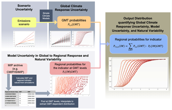
This section introduces relevant notation in Sect. 2.1, followed by the development of the RIME-X approach, which is detailed in Sect. 2.2. Section 2.3 outlines the implementation of the method within the rime Python package. Finally, we illustrate the capabilities of the RIME-X method in Sect. 2.4 by showcasing selected examples of emulations conducted with RIME-X. Figure 1 provides an overview of the RIME-X methodology.

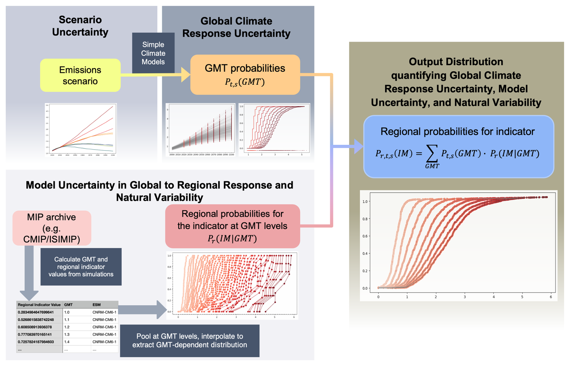
Figure 1 Schematic overview of RIME-X. We extract a scenario-specific GMT distribution from an SCM simulation ensemble and a GMT-specific distribution of a regional indicator from MIP data. Afterwards, we combine the two distributions to form a scenario-specific distribution of the regional indicator. RIME-X estimates quantiles of this output distribution by applying a Monte Carlo sampling procedure to both the GMT and indicator distributions.

2.1 Notation

Climate simulations for a given emissions scenario s, initial condition e, simulated by model m can be formally represented as tensors

$${\left(V_{\mathrm{1}},\mathrm{\dots },V_n\right)}_{\mathrm{lat},\mathrm{lon},\mathrm{t},\mathrm{s},\mathrm{m},\mathrm{e}},$$

where each variable V_i (e.g., temperature, precipitation) is defined at spatial coordinates (lat, lon) and time t. To investigate and quantify the development of the regional climate, we look at time series IM${}_{\mathrm{t},\mathrm{s},\mathrm{m}}$ of indicators IM, defined as functions

$$\mathrm{IM}=F\left(V_{\mathrm{1}},\mathrm{\dots },V_n\right),$$

and aggregated over a specific region r. An indicator IM may represent a direct climate variable, such as monthly temperature; an impact-relevant compound indicator, such as the wet bulb globe temperature; or an impact indicator derived from an external impact model (e.g., a hydrological model), which is forced with the climate variables simulated by the ESM and which outputs quantities such as projected flood depths. The aggregation typically consists of a weighted average or sum over the relevant grid points within a region over a time period. A region may represent a country, an administrative unit, or a single grid cell. The resulting time series describes how a model simulates climate conditions or their impact in a region under the specified scenario.

2.2 RIME-X

RIME-X is designed to probabilistically emulate the response of IM to arbitrary emission scenarios s as a distribution quantifying the associated uncertainties. Formally, RIME-X aims to approximate all quantiles V_p of the distribution of the regional indicator IM, defined by

$$P_{\mathrm{s},\mathrm{y}}\left(\mathrm{IM}\le V_p\right)=p,$$

where P_s,y denotes the quantile function of IM under emissions scenario s, in year y and $p\in [\mathrm{0},\mathrm{1}]$ is the corresponding quantile level. The resulting distribution incorporates (i) global climate response uncertainty represented by an ensemble of SCM simulations and (ii) model and natural variability in the mapping from GMT to IM derived from ESM simulations in a MIP (e.g. CMIP or ISIMIP; Eyring et al., 2016; Warszawski et al., 2014), referred to as the training dataset. The estimation of the quantile V_p in RIME-X is based on all values of IM simulated in the training dataset and all plausible GMT trajectories generated by the SCM ensemble for the target scenario s. RIME-X proceeds through the following three steps, utilizing a discretization of the GMT variable as described in Sect. 2.2.1:

1. Sampling GMT: draw GMT samples from a discretized prior GMT distribution for the scenario s and year y with probabilities P_s,y(GMT), derived from the SCM ensemble as detailed in Sect. 2.2.2.

2. Sampling IM values conditioned on GMT: for each GMT sample, draw corresponding samples of IM from a distribution of IM conditional on the GMT variable with probabilities P(IM∣GMT). The conditional distribution is estimated from all values of IM simulated in the training dataset, with each value weighted according to the ESM that produced it, as detailed in Sect. 2.2.3 and 2.2.4.

3. Quantile estimation: compute the quantile V_p from the IM samples. As outlined in Sect. 2.2.5, RIME-X is effectively an application of the law of total probability, which ensures that the samples of IM behave like samples from the marginal distribution with probabilities $P_{\mathrm{s},\mathrm{y}}\left(\mathrm{IM}\right)=\sum _{\mathrm{GMT}}P(\mathrm{IM}\mid \mathrm{GMT})\cdot P_{\mathrm{s},\mathrm{y}}\left(\mathrm{GMT}\right)$.

Using a GMT distribution extracted from SCM simulations as a prior to constrain the conditional distribution of IM, derived from weighted MIP data, is expected to help mitigate challenges commonly associated with the probabilistic interpretation of conventional MIP-derived distributions – such as the hot model problem (Hausfather et al., 2022) and model interdependencies (Brunner et al., 2020b).

2.2.1 Discretization of the GMT variable

To approximate both the prior probability for the GMT and the conditional probabilities P(IM|GMT) (without assuming any specific functional forms), we first divide the entire simulated range of GMT from the training dataset into evenly spaced bins of size ΔT; in practice, we typically set ΔT=0.1 K. These bins are denoted as GMT-bins B_GMT(i) and span the entire range from min(GMT) to max(GMT) as observed in the training dataset. As explained in Sect.  2.2.2, 2.2.3, and 2.2.5, this binning procedure enables the sampling of GMT values according to discrete probabilities associated with each bin and allows the construction of a conditional distribution for IM conditioned on discretized GMT values.

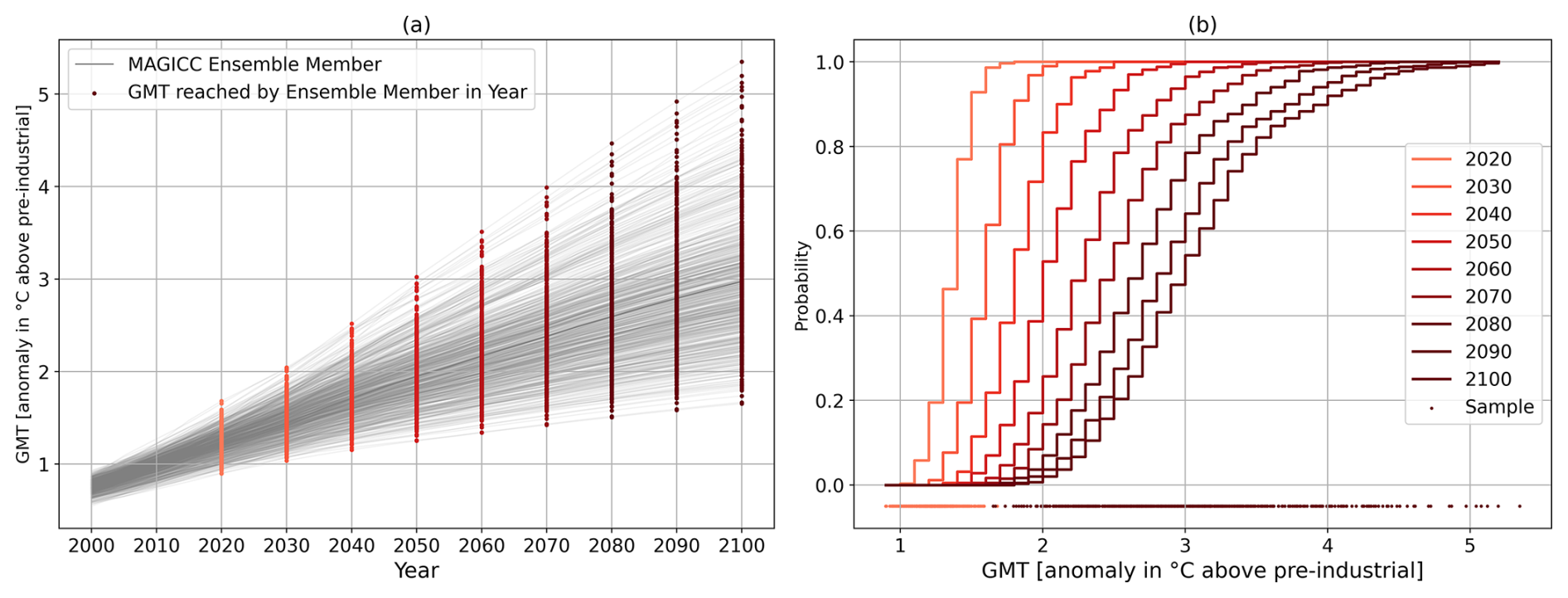
Figure 2 GMT outcomes for 600 ensemble simulations generated with the simple climate model MAGICC for the Climate Action Tracker's current policy scenario are (a) depicted as time series highlighting the GMT levels reached in each simulation in decadal steps and (b) as the corresponding cumulative distribution functions. The dots on the x axis in (b) show the GMT levels reached in the respective MAGICC ensemble simulations in 2020 and 2100, which are used for the approximation. The step form of the CDF stems from the discretization of the GMT variable.

2.2.2 Approximating the GMT distribution from SCM ensemble simulations

To quantify global climate response uncertainty to emissions, we approximate the likelihood that in the emissions scenario s and year y a certain GMT level is reached using SCMs such as MAGICC and FaIR, run for the given emissions scenario. SCMs translate greenhouse gas emissions into pathways for globally defined atmospheric variables such as the GMT using a simple carbon cycle model, a set of energy balance equations, distributions of climate system properties from the scientific literature, and observational constraints. They can also be expanded to simulate important variables from other Earth system components such as mean global sea level rise (Meinshausen et al., 2011a, b; Nauels et al., 2017; Leach et al., 2021).

However, as some key climate system properties of the Earth influencing the global climate response to emissions cannot be unambiguously determined, SCMs run many times, making differing plausible assumptions about the values of these properties. As a result, they generate a set of plausible trajectories of certain global variables (primarily GMT), which is probabilistically interpretable due to their systematic parametrization process and can be used to quantify parameter uncertainty in the global climate response of the Earth system to the emissions scenario. Formally, SCMs provide their output as a set of ensemble simulations GMT($y,s,e$) for years y, emission scenario s and ensemble members e∈E (which differ from other ensemble members by making different underlying assumptions on the climate system properties). Figure 2a shows an example for such an ensemble simulation. From this data we can approximate the probability of each GMT level being reached in year y and emission scenario s by simply counting the number of ensemble members for the SCM simulation of scenario s that lie in a given predictor bin of size ΔT in year y and dividing it by the total number of ensemble members $\left|E\right|$, thus

$$\begin{array}{ll}{\displaystyle }P(\mathrm{GMT}{)}_{\mathrm{s},\mathrm{y}}& {\displaystyle }=P_{\mathrm{s},\mathrm{y}}\left(T_i\le \mathrm{GMT}<T_i+\mathrm{\Delta }T\right)\\ {\displaystyle }& {\displaystyle }\approx {\displaystyle \frac{\left|\left\{e\left|\mathrm{GMT}\right(y,s,e)\in B_{\mathrm{GMT}}(i)\right\}\right|}{\left|E\right|}}.\end{array}$$

Here, (T_j)_{j=1 … N} form an evenly spaced partition of the temperature range in the calibration dataset, where N is the number of bins. Each temperature bin B_GMT(j) contains all GMT values x satisfying $T_j\le x<T_j+\mathrm{\Delta }T$. The index i in the equation for P(GMT)_s,y denotes the bin corresponding to the GMT value under consideration. An example of a cumulative distribution function derived with this method can be seen in Fig. 2b.

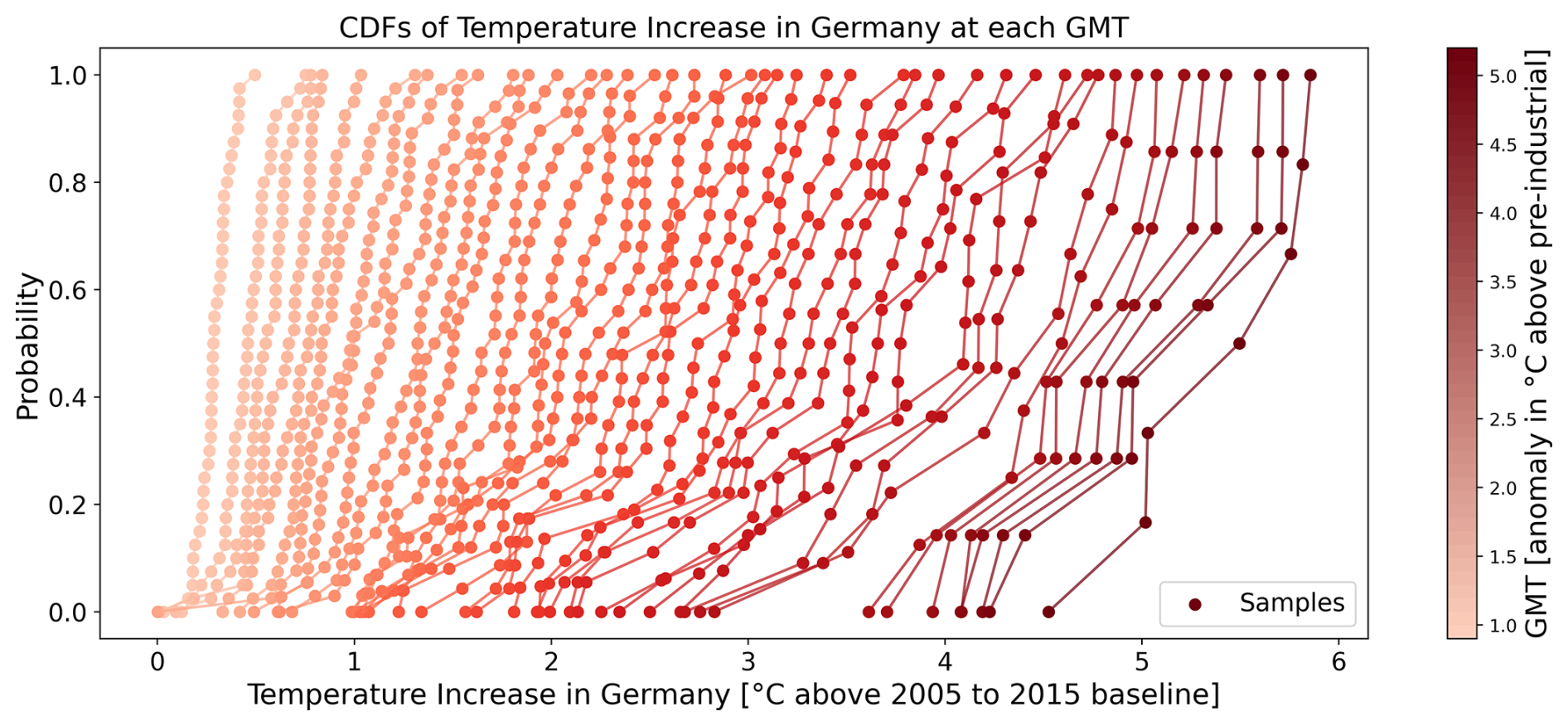
Figure 3 Approximations of the conditional cumulative distribution functions (CDFs) of a regional impact (here the 21-year mean of regional temperature in Germany compared to the 2005 to 2015 baseline) at each GMT level. It is extracted from a subset of the ISIMIP3b input simulations for the tas variable using equal model weighting. The points correspond to samples taken from the ISIMIP simulations.

2.2.3 Approximating the distributions of regional indicators conditioned on GMT

To estimate the probability of IM conditioned on the discretized GMT level that quantifies model uncertainty in the response of IM to global climate conditions, we first collect all simulated values for IM from the training dataset along with the discretized GMT level at the time the value is simulated. In a second step we group all values for IM in bins B_IM(GMT) according to their corresponding GMT levels. We finally assign a weight to all values within each bin according to the ESM they were simulated with using a selected model weighting scheme (see in Sect. 2.2.4). We obtain the final conditional probabilities P(IM∣GMT) of values of IM conditioned on the discretized GMT variable using weighted linear interpolation between the values grouped into each individual bin. Figure 3 shows the cumulative probability functions of the resulting conditional distribution for the 21-year mean of regional temperature in Germany compared to the 2005 to 2015 baseline at each GMT level, as extracted from a subset of the ISIMIP3b input simulations of the temperature at surface (tas) variable using equal model weighting. Note that grouping values of IM into bins B_IM(GMT), extracting the corresponding conditional distributions, and defining probabilities for GMT levels as in the previous section, is enabled by the discretization of the GMT variable.

2.2.4 Model weighting approaches

When using MIP datasets like CMIP6 or ISIMIP as a training dataset, one has to consider that different models do not necessarily contribute the same number of simulations to those datasets. As a result, the number of values for IM contributing to each bin B_IM(GMT) sourced from each model can vary significantly. This variation can lead to an unequal influence of each model on the conditional distribution P(IM∣GMT). For instance, models that provide more data, either through additional initial condition ensembles or by covering a wider range of scenarios, would have a greater impact on the conditional distributions without model weighting because they contribute more values to the bins, thereby skewing the distributions. To address this bias towards models with more simulations, we implement a weighting mechanism that assigns a weight w_m,s based on the source of each value defined by the model m and simulation s. We implement the following three weighting strategies:

• Simulation democracy corresponds to applying no extra weighting, which results in each simulation having equal influence on the conditional distribution. Consequently, models providing more simulations, either in the form of more initial condition ensembles or covering more input scenarios, have a larger overall impact.

• Model democracy ensures that each source model has an equal influence on the conditional distribution. In this approach, simulations from models contributing a larger total number of simulations to the training dataset are given lower weights so that each model has the same impact.

• Manual weighting can be combined with the other approaches and allows users to manually assign weights to individual models or simulations. This method can be used to implement model weighting strategies from the scientific literature into RIME-X, which weight models e.g. by how well their simulation of the historical period matches with observations or by how independent the models are from each other (Palmer et al., 2023; Massoud et al., 2023; Brunner et al., 2020b). Manual weighting can also be used to select simulations that capture particular events, such as an AMOC slowdown.

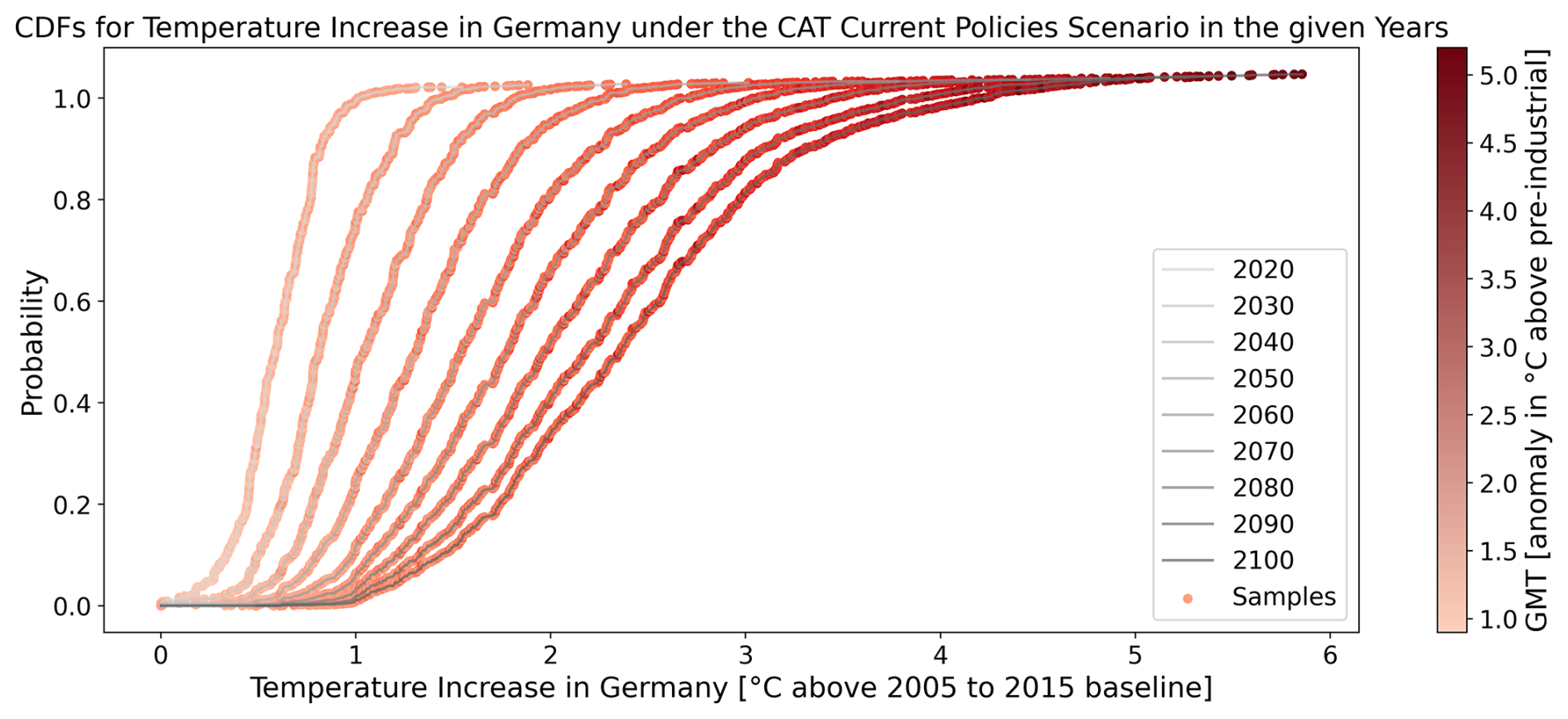
Figure 4 Cumulative distribution functions (CDFs) for the regional impact (here the 21-year mean of regional temperature in Germany compared to the 2005 to 2015 baseline) in the years 2020–2100 when following Climate Action Tracker's current policy scenario. The shown distribution is a weighted sum of the regional temperature distributions in Fig. 3, where the weights are given by the probabilities of each GMT level in each year (see Fig. 2b). Each point corresponds to a sample of the indicator extracted from ISIMIP simulations. The color of the point denotes the GMT level in the simulation at the time the sample was extracted. The applied weighting strategy is simulation democracy.

2.2.5 Calculating the final quantiles of the regional indicator distribution

To estimate the quantiles V_p of the distribution of IM, we apply Monte Carlo sampling. Specifically, we draw n samples of GMT levels with probabilities P_s,y(GMT). For each sampled GMT level, we then draw one value IM with probability P(IM∣GMT). This results in a set of n samples of IM, from which we compute empirical quantiles. The sampling procedure ensures that the IM values are drawn with probability

$$P_{\mathrm{s},\mathrm{y}}\left(\mathrm{IM}\right)=\sum _{\mathrm{GMT}}P(\mathrm{IM}\mid \mathrm{GMT})\cdot P_{\mathrm{s},\mathrm{y}}\left(\mathrm{GMT}\right),$$

which represents an application of the law of total probability. Consequently, empirical quantiles derived from the sample set provide a close approximation to the true quantiles of the marginal distribution of IM. Figure 4 illustrates the resulting marginal distribution for the 21-year mean of regional temperature in Germany (relative to the 2005–2015 baseline), constructed using the prior GMT-distribution displayed in Fig. 2 and the conditional IM-distribution presented in Fig. 3. The number of samples n is a hyperparameter of the RIME-X method. By default, we set n=10 000.

2.3 Implementation

The RIME-X emulator is implemented as an extension of the existing rime Python package (Byers et al., 2025). It includes a preprocessing pipeline designed to facilitate the data handling for emulation tasks, with built-in support for downloading simulation output from the ISIMIP repository. The pipeline can also be applied to other MIP datasets, provided they are manually preprocessed into a similar structure as the downloaded ISIMIP dataset. In the first step, the required data is downloaded and converted into NetCDF files containing the target indicator IM in a gridded format, at the minimum necessary temporal resolution. This gridded data is then aggregated regionally using predefined spatial masks. By default, the package includes masks for continents, countries, provinces, and scientifically relevant regions like the IPCC regions (Iturbide et al., 2020), with aggregation weighted by area, GDP, or population. Users may also supply custom regional masks. The regionally aggregated data is transformed into NetCDF files, we call quantile maps with dimensions for GMT level, quantile, and region, encoding the conditional distributions described in Sect. 2.2.3. Alternatively, the package supports transformation into grid-point-level quantile maps, with dimensions GMT level, quantile, and spatial coordinates. In this work, we use 101 equally spaced quantile levels (corresponding to the integer percentiles 0–100) and 0.1° temperature increments. For quantile emulation, the package provides a dedicated function. It takes as input an ensemble simulation of GMT for a given scenario, a list of years and quantiles of interest, and the regional conditional distribution data preprocessed in the described format. The function returns the requested quantiles of the indicator IM for the specified scenario, years, and regions. In practice, this function first samples a GMT value from the SCM ensemble and a quantile from the quantile map. It then obtains the regional indicator sample by linearly interpolating between the quantile values of the indicator distributions conditional on the two nearest GMT values to the GMT sample in the quantile map, so no temperature binning is needed during prediction.

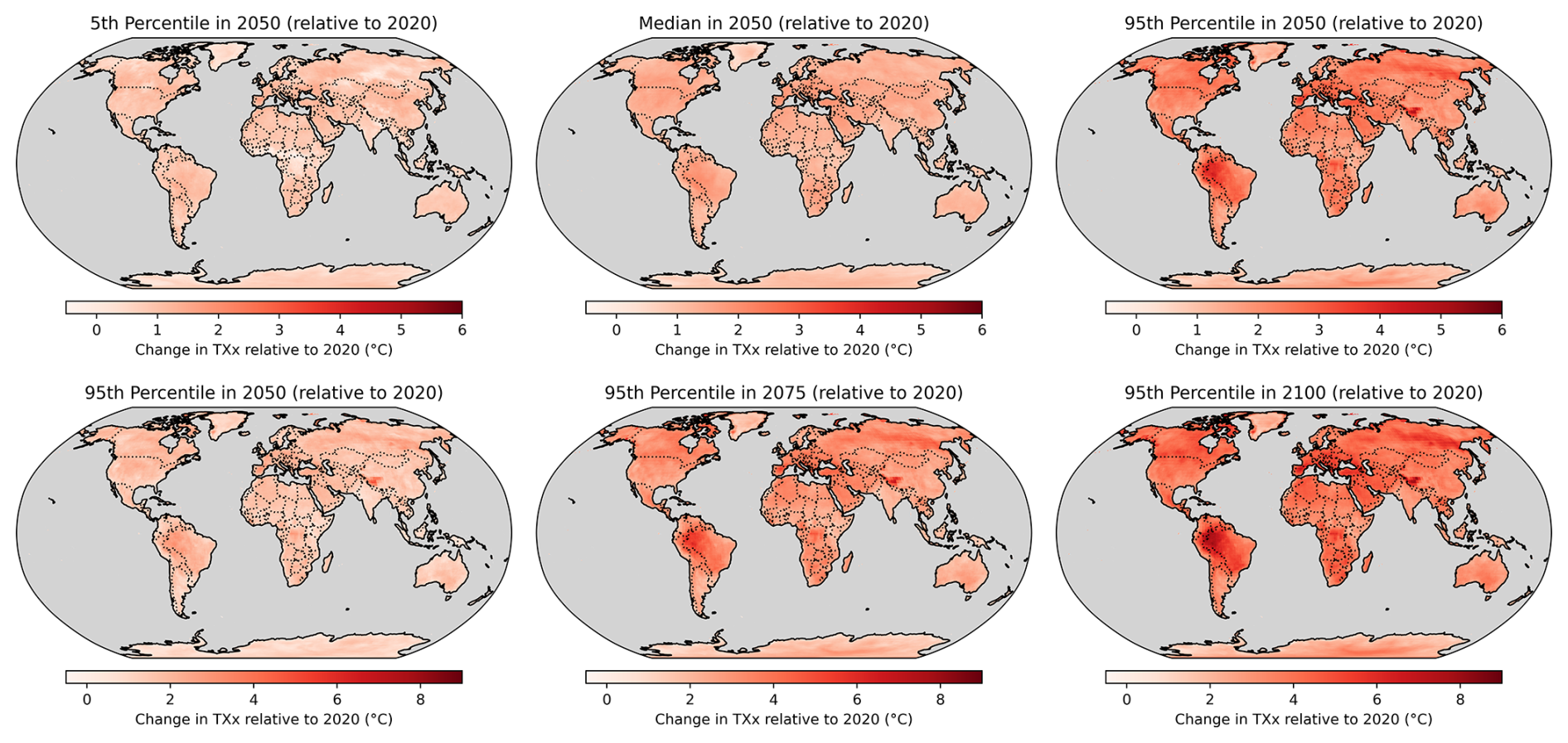
Figure 5 Grid-point-level RIME-X emulations for the CAT Current Policies scenario, illustrating the distribution and temporal evolution of annual maximum temperature (TXx). The upper panel shows the median as well as the 5th and 95th percentiles of the indicator distribution in 2050. The lower panel presents the 95th percentile of the distribution for the years 2050, 2075, and 2100, highlighting changes in both magnitude and spatial extent over time.

2.4 Showcase

Here we present selected examples of emulations produced by RIME-X to illustrate its capabilities in capturing the shift in distributions of regional climate indicators. We focus on the Climate Action Tracker (CAT) Current Policies scenario, which exhibits a strong climate signal across various indicators due to its high degree of projected warming. The GMT distribution used as input for the emulations is derived from an ensemble simulation using the simple climate model MAGICC. To highlight the capabilities of RIME-X, we present the emulated outputs using a variety of visualization formats. Figure 5 provides a grid-point-level representation of selected percentiles of the emulated distributions of the annual maximum daily maximum temperature indicator (TXx), shown relative to the 2020 median. The upper panel presents the 5th, 50th, and 95th percentiles for the year 2050. The lower panel focuses on the 95th percentile in 2050, 2075, and 2100, highlighting temporal shifts in extreme heat conditions. In Fig. 6, we focus on the temporal evolution of regional indicator distributions. On the left-hand side, we display how the density functions of distributions of selected indicators shift from 2020 to 2100 under the CAT Current Policies scenario. These distributions are approximated by applying a Gaussian kernel density estimate (KDE) to each quantile emulated by RIME-X. On the right-hand side, we show the evolution of the emulated quantiles over time. We highlight the median and the 90 % confidence interval. To emphasize the flexibility of RIME-X, we selected a diverse set of emulation cases. Results are shown for a variety of spatial region types and locations (e.g., countries such as Germany and Mexico, provinces such as Guangdong, and IPCC regions such as Southeastern Africa); various indicator types, including indicators taken directly from the ISIMIP data (mean annual temperature), indicators derived from ISIMIP data (cooling degree days and extreme precipitation), and indicators generated using impact models (maize yield change). The underlying indicator simulations were obtained from the ISIMIP3 repository, using all available simulations (including secondary input) and preprocessed with a 21-year running mean to reduce the effect of natural variability, leading to smoother distributions representing mainly the climatic trend in the indicator. A more detailed description of the specific indicators used can be found in Appendix B, and an evaluation of the RIME-X emulator for the indicators is presented in Appendix D.

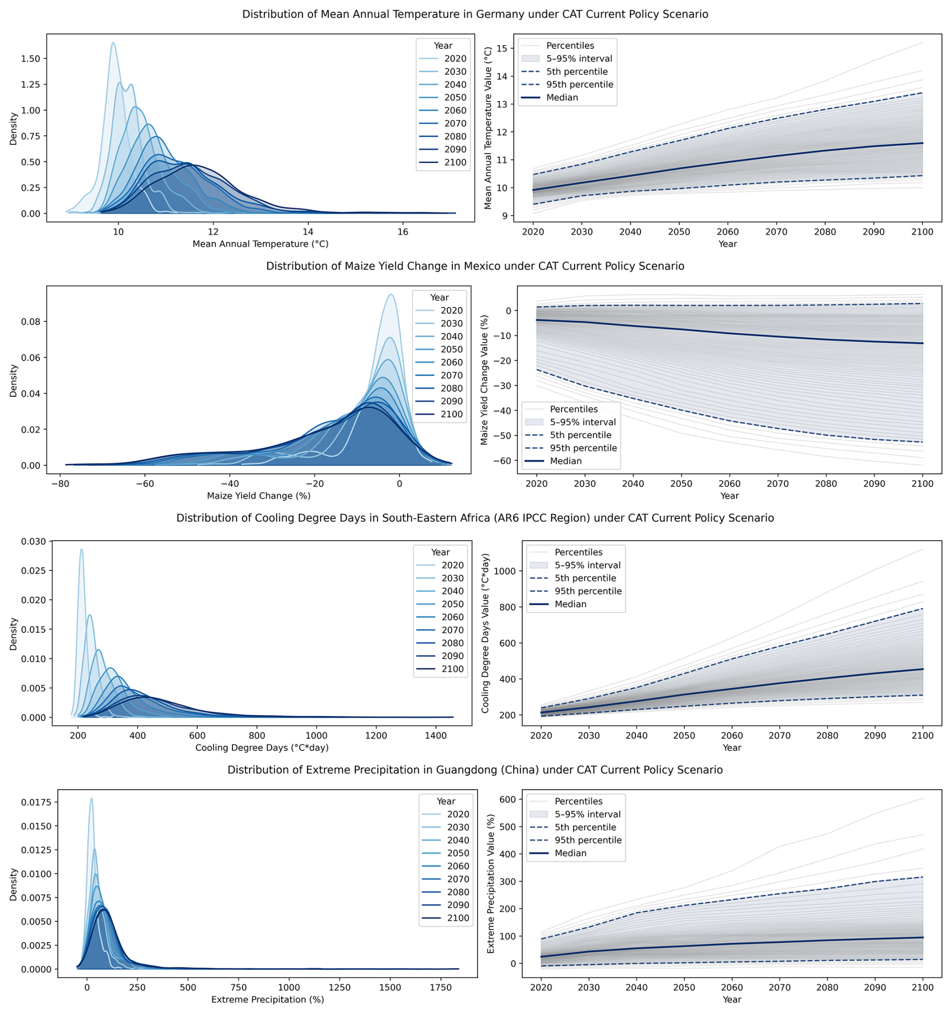
Figure 6 Four examples of RIME-X emulations of the CAT Current Policies scenario illustrating different indicator–region combinations. For each case, the left panel shows the evolution of the indicator distribution over time, while the right panel presents a time series of the percentiles from those distributions. Overall, the distributions tend to widen over time and shift in the direction of the underlying trend, reflecting both increasing model and global climate response uncertainty as well as the projected signal.

3 Discussion and validation

This section discusses the limitations of the methodology of RIME-X in Sect. 3.1, which motivates the development and implementation of an empirical validation strategy in Sect. 3.2.

3.1 Methodological limitations of RIME-X

To develop a validation strategy for RIME-X, we first identify potential conceptual limitations in its methodology. The first step of RIME-X – translating an emissions scenario into a GMT distribution using SCMs – follows established climate science as applied in recent IPCC assessments (e.g. Forster et al., 2021; Riahi et al., 2022). SCMs are highly simplified representations of the climate system that are calibrated against historical observations and have been shown to reproduce the historical period well. Comparisons of SCM projections with ESM projections – our current best tools to project the evolution of the future climate – find no major structural limitations for the GMT variable relevant to the RIME-X framework. However, such evaluations primarily assess consistency with ESM behavior rather than the absolute accuracy of SCM projections and underlying ESM behavior, which means that such validation still cannot guarantee that their application to future climate states delivers adequate projections (Nicholls et al., 2020, 2021; Forster et al., 2021). SCMs guard against overconfidence in projections by simulating large ensembles based on systematically generated, historically constrained probabilistic parameter sets. The parameterization process samples a wide range of plausible responses in key physical processes – such as land–atmosphere interactions and ocean carbon uptake – typically designed to encompass the IPCC-assessed uncertainty ranges (Meinshausen et al., 2011a, b; Smith et al., 2024). These uncertainties are explicitly propagated within RIME-X to inform regional impact projections across multiple emissions scenarios. While we acknowledge that SCMs have inherent limitations, such as unresolved or potentially misrepresented processes following from the strong simplifications in the model structure, they currently provide the best available probabilistic estimates of GMT responses to emissions. The use of probabilistic ensembles that cover IPCC-assessed ranges also guards against introducing bias in any single direction. Given their extensive validation and assessment elsewhere, we consider validation of SCM-based projections to be beyond the scope of this study and treat SCM-based projections as established climate science.

The second step – deriving GMT-conditioned regional indicator distributions from MIP datasets – presents the main methodological challenge. Here, regional indicator values are binned by GMT to extract conditional distributions, assuming path independence, meaning that changes of regional indicator distributions from climate change depend entirely on the level of GMT, while the trajectory taken to reach that level of GMT and other regional influences like aerosol levels or deforestation are not taken into account. Though supported and applied in the literature for many indicators (Herger et al., 2015; Schleussner et al., 2016; Hausfather et al., 2022), this assumption can introduce biases, particularly for overshoot or stabilization scenarios, and in regions or indicators affected by pattern effects, high regional aerosol concentrations, changing circulation patterns, land–atmosphere feedbacks, SST-driven pattern effects, monsoon dynamics, or changes in regional land use (Schleussner et al., 2024; Pfleiderer et al., 2024; Wells et al., 2023; Giani et al., 2024). These limitations also restrict the applicability of our approach to idealized model experiments deploying solar radiation modification. However, when all scenarios and years of a training dataset are included in the calibration, any loss of predictability due to time lag or related effects will manifest as increased uncertainty (i.e., wider error bars) rather than as an overconfident estimate, as long as the emulated scenario is not a strongly out-of-sample case with respect to the training data, for example, when emulating scenarios involving high-overshoot pathways using a training dataset that does not include such processes. Additional limitations stem from the data: MIP ensembles offer a limited number of simulations, often developed using models that share components and are best viewed as “ensembles of opportunity” (Masson and Knutti, 2011; Brunner et al., 2020b; Knutti et al., 2010). While RIME-X can mitigate some of these limitations through model weighting, the underlying epistemic uncertainties persist (Rising et al., 2022; Stainforth et al., 2007). Moreover, many models in the MIP dataset do not reach higher levels of warming, meaning that the regional indicator distributions conditioned on these higher GMT levels are based on an increasingly small and selective subset of models that can provide data at these temperatures. This effect is partly mitigated by the fact that global climate response uncertainty increases with higher emission levels, leading to a wider range of simulated GMT outcomes. As a result, higher-emission scenarios generally sample a broader span of GMT levels, which counteracts – at least to some extent – the reduction in available samples for any specific high-GMT bin. The inclusion of high-warming scenarios such as SSP5-8.5 in the training data also provides additional coverage at high-GMT levels. Despite these limitations, MIPs remain the most holistic and flexible datasets for linking global and regional climate responses and are thus the best available foundation for RIME-X’s emulation approach, which is designed to be flexible across regions, scenarios, and indicators. The third and final step of RIME-X is a direct application of the law of total probability.

In summary, the first and third steps of RIME-X either rely on well-established methodologies or are mathematically valid. Accordingly, our empirical validation in Sect. 3.2 focuses on the second step: evaluating whether GMT-conditioned regional distributions extracted from MIP datasets can reliably reproduce simulated regional outcomes. This analysis does not, and cannot, address the epistemic limitations of MIP data. Instead, we treat MIP-derived distributions as ground truth and assess whether they can be reconstructed based solely on their dependence on GMT.

3.2 Empirical validation strategy using CMIP6 data

To investigate how reliably RIME-X emulates simulated distributions using GMT-conditioned regional indicator distributions, we adopt a holdout validation framework. The emulator is calibrated on a subset of simulations from CMIP6 (Eyring et al., 2016), withholding all simulations of the test scenario. As test scenarios, we use SSP1-2.6, SSP2-4.5, and SSP3-7.0, which we aim to emulate. For both calibration and ground truth, we use data from the CMIP6 next-generation archive (Brunner et al., 2020a), which has undergone centralized preprocessing, including interpolation to a common 2.5°×2.5° latitude-longitude grid. This archive provides over 1500 simulations from 48 models (see Appendix A) covering the historical period and the emissions scenarios SSP1-2.6, SSP2-4.5, SSP4-6.0, SSP3-7.0, and SSP5-8.5, enabling robust calibration of the RIME-X emulator, including in our holdout validation framework. The archive additionally offers more than 150 simulations of each of the test scenarios from the same set of models, which allow us to extract statistically meaningful ground truth quantiles from actual simulations for comparison with our emulated quantiles. For emulator calibration and ground truth preprocessing, the CMIP6 simulations are spatially aggregated to the country level using masks from the ISIMIP archive (Perrette, 2022) and area-based grid cell weights. Temporal aggregation is then performed by applying a 21-year running mean to the regional averages in order to reduce sample uncertainty in the ground-truth distribution and make it comparable to the emulated distribution. This aggregation reduces the impact of outliers arising from natural variability, as the ground-truth distribution is estimated from significantly fewer samples per year than the emulated distribution. Countries are chosen as regions for the evaluation due to their heterogeneous sizes, diverse climate zones, and global landmass coverage, thus testing the method’s applicability across varied regional characteristics. Only simulations from the scenarios SSP1-2.6, SSP2-4.5, SSP4-6.0, SSP3-7.0, and SSP5-8.5 that are not simulations of the test scenario and share a model and initial condition ensemble with a simulation of the test scenario (including their respective historical simulations) are used to calibrate the RIME-X emulator. We give equal weight to every simulation (see Sect. 2.2.4). All available CMIP6 simulations for the test scenarios are used to derive the ground truth distributions. To ensure comparability between emulated and simulated distributions, we use the actual global warming levels from the test scenario simulations to extract the scenario-dependent GMT distribution instead of using an SCM. This departs from the standard RIME-X methodology, which would otherwise rely on warming levels from SCM ensemble simulations (see Sect. 2.2.2). However, SCM ensembles are designed to simulate realistic warming trajectories by assuming observation-based values for key metrics like the transient climate response (Leach et al., 2021), whereas many CMIP6 models tend to overestimate transient warming rates (Hausfather et al., 2022). Using the same warming levels as the ground truth simulations ensures that deviations between emulated and simulated distributions arise solely from the second step of the emulation methodology, rather than differences in warming trajectories. Consequently, if the emulated distributions closely match the simulated ground truth, we can conclude that RIME-X can use the relationship between GMT levels and regional indicators extracted from the CMIP6 simulations to produce meaningful regional indicator distributions for the unseen scenario.

3.2.1 Results and discussion

Figure 7 shows the average normalized mean absolute error (ANMAE) of each percentile of the emulated distribution compared to the corresponding percentiles of the ground-truth simulated distribution for each country. Results are shown for (a) annual average regional surface temperature relative to the 1995–2014 baseline under SSP2-4.5 (in °C), and (b) annual average regional precipitation relative to the same baseline and scenario (in percent). The average normalized mean absolute error ANMAE_r for region r quantifies the error between the emulated p-percentiles $e_{\mathrm{y}}^{\mathrm{r}}\left(p\right)$ (where p is a whole number between 1 and 99) in the years y∈Y (here ranging in 5-year steps from 2025 to 2090) and the corresponding simulated percentiles $s_{\mathrm{y}}^{\mathrm{r}}\left(p\right)$. The ANMAE_r is calculated as

$$\begin{array}{}\text{(1)}& {\mathrm{ANMAE}}_{\mathrm{r}}={\displaystyle \frac{\mathrm{1}}{\left|Y\right|}}\sum _{\mathrm{y}\in \mathrm{Y}}{\displaystyle \frac{\sum _{p=\mathrm{1}}^{\mathrm{99}}\left|e_{\mathrm{y}}^{\mathrm{r}}\right(p)-s_{\mathrm{y}}^{\mathrm{r}}(p\left)\right|}{\max s_{\mathrm{y}}^{\mathrm{r}}\left(p\right)-\min \left|s_{\mathrm{y}}^{\mathrm{r}}\right(p)}}.\end{array}$$

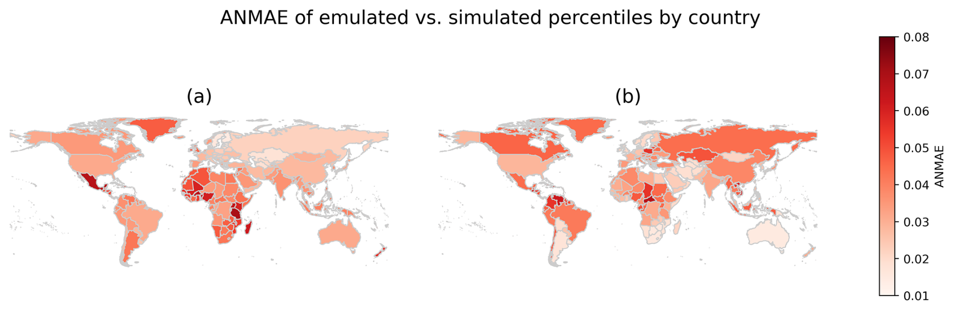
Figure 7 The average normalized mean absolute error (ANMAE, see Sect. 3.2.1) of emulated vs. simulated percentiles in each country. Panel (a) shows the annual average regional surface temperature compared to the 1995–2014 baseline for SSP2-4.5 in °C, and panel (b) shows the annual average regional precipitation compared to the 1995–2014 baseline for SSP2-4.5 in percent.

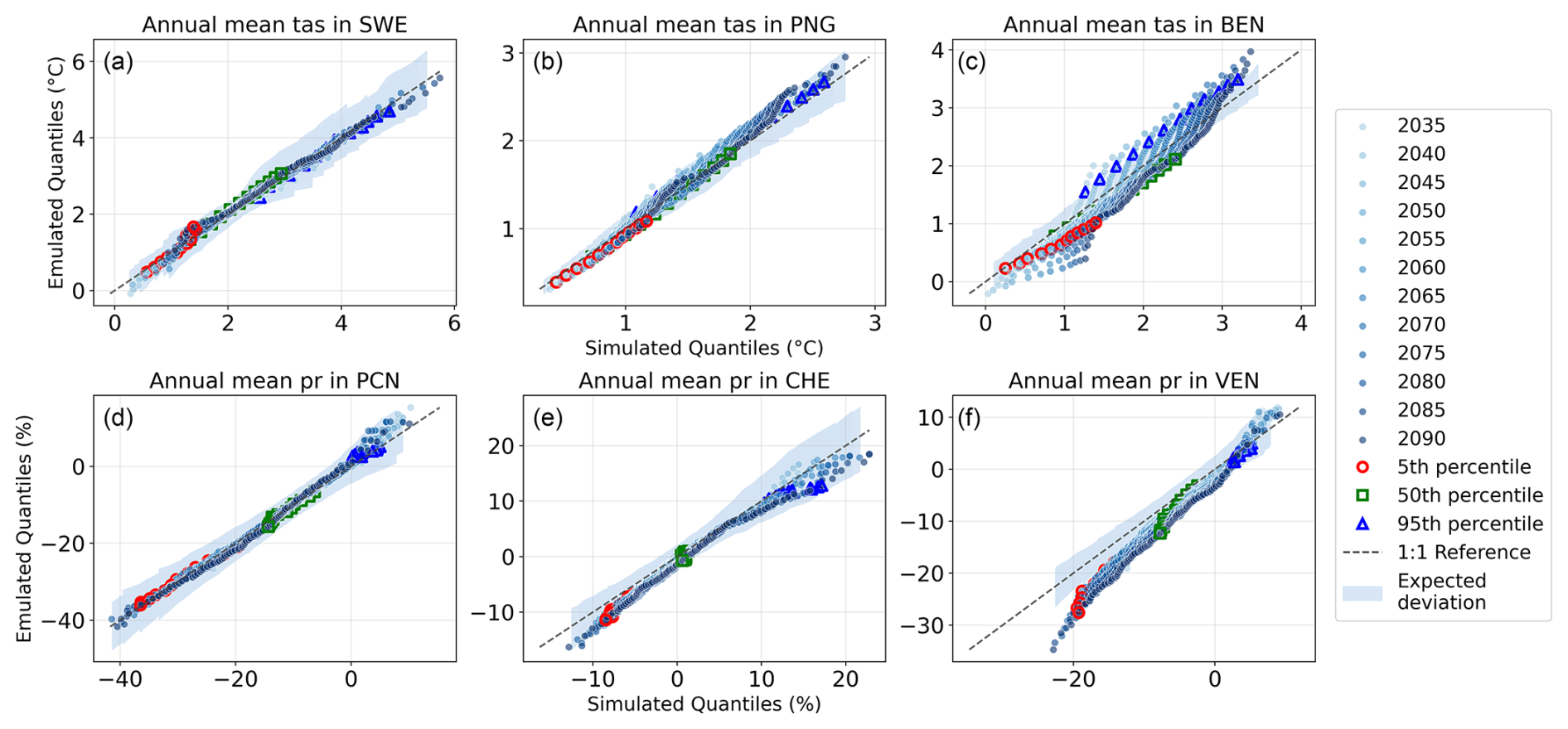
Figure 8 Q–Q plots showing the emulated and simulated percentiles from the CMIP6 ensemble. A perfect emulator and perfect knowledge of the simulated distribution would result in all points lying on the diagonal line included in the Q–Q plot. However, even if RIME-X were perfect, we would still expect a deviation of the emulated percentiles from the simulated percentiles as a result of the imperfect knowledge of the simulated distribution we have to estimate from around 150 samples. The expected deviation is quantified in the shaded area. While agreement across all percentiles is desirable, deviations in the tails are particularly important, as accurate representation of extremes is critical for many impact assessments. From left to right the examples illustrate the emulator performance for regions where the emulator showed the best, median, and worst performance as measured by the average normalized mean absolute error (ANMAE, see Sect. 3.2.1). In the first row we show the emulated and simulated percentiles of the annual average regional temperature (tas) compared to the 1995–2014 baseline in °C for selected regions, where (a) corresponds to Sweden (SWE), (b) to Papua New Guinea (PNG), and (c) to Benin (BEN). In the second row we show the emulated and simulated percentiles of the annual average regional precipitation change indicator (pr) in °C for selected regions, where (d) corresponds to Pitcairn (PCN), (e) to Switzerland (CHE), and (f) to the Venezuela (VEN).

This metric represents the average deviation of each emulated percentile from its corresponding ground truth simulated percentile, expressed as a share of the full spread of simulated indicator values. We find that over all countries and both indicators, the ANMAE between the emulated and simulated quantiles ranges from 1 % of the model spread to 8 % of the model spread. For the regional temperature indicator investigated in Fig.  7a, Sweden has the lowest ANMAE of around 1.4 %, Papua New Guinea has the median ANMAE value of 3.8 %, and Benin has the maximum ANMAE value of 6.5 %. For the regional precipitation indicator investigated in Fig.  7b, Pitcairn has the lowest ANMAE of around 1.4 %, Switzerland has the median ANMAE of around 3.2 %, and Venezuela has the maximum ANMAE of 6.2 %. Figure 8 displays Q–Q plots comparing the percentiles of the emulated and simulated distributions for each year. The plots reveal some deviations between the emulated and simulated quantiles. However, such deviations are partially expected, as the 98 percentiles of the simulated distribution are estimated from only around 150 samples – a relatively small sample size that introduces uncertainty in the ground truth quantiles. As a result, even a perfect emulator would still exhibit some deviation in the Q–Q plots due to this sampling variability. To quantify the magnitude of the expected deviations due to the sample size, we estimate the simulated ground truth distribution using a Gaussian kernel density estimate. From this estimated distribution, we repeatedly (1000 times) draw sets of 100 samples and compute the percentiles for each sample set. We then record the range within which the percentiles from these samples deviate from the percentiles of the simulated distribution. This range represents the expected deviation due to the unstable estimation of the ground truth from a limited number of samples and is added to Fig. 8 as a bright blue shadowing. We observe that while emulated and simulated quantiles mostly fall within the expected range of sampling deviations, they exceed this range in some cases. This suggests that the methodological limitations discussed in Sect. 3.1 can introduce systematic biases. However, as shown in Fig. 7, these biases remain modest, with average deviations typically reaching between two and six percent of the model spread and reaching at most around eight percent even in the worst-affected regions. Overall, deviations between emulated and simulated ground-truth distributions remain one to two orders of magnitude smaller than the inter-model spread in CMIP6 and are often within the range of expected deviations due to the limited sample size from which the ground-truth quantiles are extracted.

To investigate the effect of potential sources of bias on RIME-X, we repeat the validation framework using SSP1-2.6 and SSP3-7.0 as test scenarios, while training the emulator on the remaining scenarios. SSP1-2.6, with its slight overshoot and prolonged stabilization period, provides a useful test case for assessing biases arising from path dependence, including changes in circulation patterns, land–atmosphere feedbacks, SST-driven pattern effects, and monsoon dynamics. In contrast, SSP3-7.0 allows us to evaluate the sensitivity of the emulator to aerosol forcing pathways that differ from those represented in the training scenarios. The resulting plots are provided in the Appendix as Figs. C1–C4.

They show that, for SSP1-2.6, biases increase, particularly for precipitation-related indicators. Minimum errors remain approximately unchanged for temperature and increase slightly for precipitation (+0.4 pp). Median errors remain approximately unchanged for temperature and increase substantially for precipitation (+1.3 pp). Maximum errors increase slightly for temperature (+0.7 pp) and more then double for precipitation (increases of up to +10 pp). The Q–Q plots (Fig. C3) indicate that the increase in maximum precipitation errors is associated with a progressive shift of the simulated distribution away from the emulated distribution over time, suggesting the presence of path-dependent effects. This behavior is consistent with the expected limitations and could, for example, be explained by continued ocean warming and associated circulation adjustments influencing regional precipitation patterns even after global mean temperatures stabilize. For SSP3-7.0, we likewise observe a moderate increase in biases, particularly in regions strongly affected by aerosol forcing changes, including parts of Africa and Asia. Minimum errors decrease slightly for temperature (−0.1 pp) and increase slightly for precipitation (+0.3 pp). Median errors increase moderately for both temperature (+0.7 pp) and precipitation (+0.9 pp). Maximum errors increase more noticeably for temperature (+2 pp) and nearly double for precipitation (up to +7 pp). The error map plots (Fig. C2) indicate that these larger deviations are concentrated primarily in regions with strong aerosol-driven circulation responses, consistent with the expected limitations of the framework when emulating a scenario with substantially different aerosol forcing than the training scenarios. Overall, these results indicate that both path dependence and aerosol forcing differences can introduce systematic deviations in the emulated distributions. However, the resulting biases remain moderate in most regions and are consistent with the discussed limitations.

4 Conclusions

We have developed and validated RIME-X, an emulator that predicts scenario- and time-dependent distributions of regional indicators under climate change. RIME-X applies to any indicator whose distribution is mainly influenced by global warming levels. Unlike ESM emulators, RIME-X emulates distributions of responses directly, integrating uncertainty in the global response to emission scenarios (via SCM ensembles), model uncertainty in the regional response to global climate change (from weighted MIP datasets), and internal climate variability (via multiple simulations from the same model). This enables efficient exploration of projected regional impacts across multi-model ensembles like CMIP6 or ISIMIP3, constrained by plausible global climate trajectories from simple climate models and model weighting to mitigate challenges commonly associated with the probabilistic interpretation of conventional MIP-derived distributions – such as the hot model problem (Hausfather et al., 2022) and model interdependencies (Brunner et al., 2020b). RIME-X is conceived to support users such as researchers and practitioners from, e.g., the finance sector who need fast, flexible, and probabilistic assessments of climate risks across scenarios, regions, and indicators. It enables the exploration of the full range of possible effects of an emission scenario on a regional indicator, including the extreme ends of the risk spectrum. We provide a user-friendly implementation of RIME-X in the Python package rime, which includes a preprocessing module that automatically downloads and processes indicators from the ISIMIP repository but also supports processing of custom indicators. We apply RIME-X in the Climate Impact Explorer (https://climate-impact-explorer.climateanalytics.org, last access: 11 November 2025), for which we have already preprocessed a wide range of indicators that will be made publicly accessible.

We validated RIME-X by calibrating it with CMIP6 simulations for four scenarios (excluding either SSP1-2.6, SSP2-4.5, or SSP3-7.0 used as test scenario) for regional temperature and precipitation. We then emulated the distribution of the CMIP6 ensemble under the test scenario using the GMT timeseries from the simulations of the test scenario and the conditional distributions extracted from the CMIP6 simulations of the other scenarios, and compared the results to the actual CMIP6 distribution extracted from the test scenario simulations, which we treat as the ground truth. Emulated and simulated distributions matched closely for SSP2-4.5, with percentile deviations averaging 1 % and up to 8 % of model spread over all countries in the best- to worst-case. However, some limitations can affect RIME-X's accuracy. It assumes that the regional indicator depends primarily on GMT, excluding influences like aerosols, shifts in socioeconomic conditions, land use, or circulation patterns (including SST-driven pattern effects, monsoon dynamics, and land-atmosphere feedbacks). This limits applicability to regions or indicators where this assumption approximately holds. It also does not account for the path to reaching GMT levels, limiting applicability in scenarios or indicators where time-lag effects play a major role for the assessment of regional indicators, such as overshoot or stabilization scenarios. In addition, the framework may be less robust in scenarios where regional aerosol forcing differs strongly from the training scenarios. Our approach is also not validated for idealized model experiments deploying solar radiation modification. Moreover, as fewer ESMs reach high warming levels, the robustness of emulations decreases with warming level due to reduced training data, making the inclusion of high warming scenarios such as SSP5-8.5 in the training data particularly important for broad applicability. A further limitation arises from the fact that the emulator is not generative: the emulated distributions are constrained by the events present in the training simulations and may therefore miss low-probability extremes that are physically plausible but not sampled. While this limitation can be mitigated by increasing the size and diversity of the training dataset, this is not always feasible. It also implies that biases or corrupted simulations in the training data can propagate into the emulator outputs. Emulations are additionally constrained by epistemic uncertainty due to the limited number of models available to quantify structural model uncertainty within the training dataset. This epistemic uncertainty is, however, partly mitigated through model weighting and GMT-based constraints. Additionally, the method does not capture temporal, spatial, or inter-variable correlations between the emulated distributions of multiple variables, regions, or time steps, even when they originate from the same underlying data source, meaning that dependencies across regions, variables, and time steps are not preserved between several emulated distributions. Finally, the applicability of the method at finer spatial scales is limited by the resolution of the underlying ESM input data, as coarse model grids may not adequately resolve smaller regions or complex boundaries. Future work could address some of these limitations – for instance, by conditioning indicator distributions on changing socioeconomic variables like GDP or population, improving robustness at high warming levels using training data with prescribed GMT shifts like, e.g., from the upcoming Tipping Points Modelling Intercomparison Project (TIPMIP; Winkelmann et al., 2025), testing additional global predictor indicators such as the likelihood of being before or after peak GMT, or extending the framework to produce multivariate output that captures spatial, temporal, or cross-indicator correlations particularly relevant for the analysis of compound events.

Appendix A: CMIP6 data used in this study

Dix et al. (2019)Ziehn et al. (2019)Semmler et al. (2019)Xin et al. (2018)Rong (2019)Swart et al. (2019a)Swart et al. (2019b)Chinese Academy of Sciences (2020)Danabasoglu (2019b)Danabasoglu (2019a)Huang (2019)Lovato and Peano (2020)Lovato et al. (2021)Voldoire (2019b)Voldoire (2019a)Seferian (2019)Bader et al. (2020)EC-Earth Consortium (2019b)EC-Earth Consortium (2020a)EC-Earth Consortium (2019a)EC-Earth Consortium (2020b)Yu (2019)Li (2019)

Table A1 First part of the overview of the CMIP6 models available in the Brunner et al. (2020a) dataset and the scenarios that are available for each model. We used this dataset in Sects. 3.2 and 3.2.1 for the validations of our method with CMIP6 data.

Song et al. (2019)Guo et al. (2018)John et al. (2018)Goddard Institute for Space Studies (2020a)Goddard Institute for Space Studies (2020b)Good (2019)Jackson (2020)Panickal et al. (2020)Volodin et al. (2019a)Volodin et al. (2019b)Boucher et al. (2020)Boucher et al. (2019)Byun et al. (2019)Kim et al. (2019)Stouffer (2019)Shiogama et al. (2019)Tachiiri et al. (2019)Schupfner et al. (2019)Schupfner et al. (2021)Yukimoto et al. (2019)Cao (2019)Seland et al. (2019)Bentsen et al. (2019)Lee and Liang (2020)Good et al. (2019)

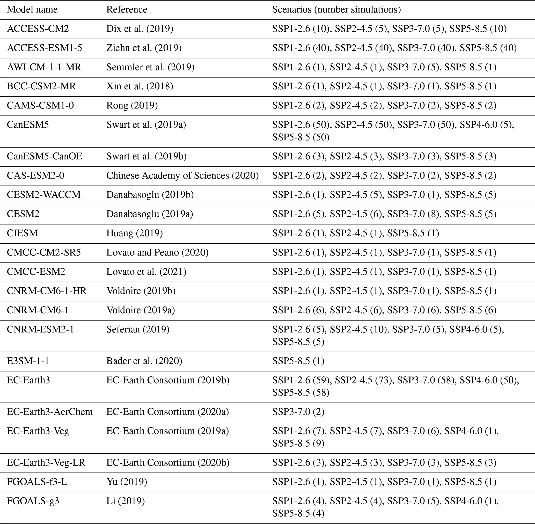
Table A2 Second part of the overview of the CMIP6 models available in the Brunner et al. (2020a) dataset and the scenarios that are available for each model. We used this dataset in Sects. 3.2 and 3.2.1 for the validations of our method with CMIP6 data.

Appendix B: Definitions of the indicators presented in the showcase

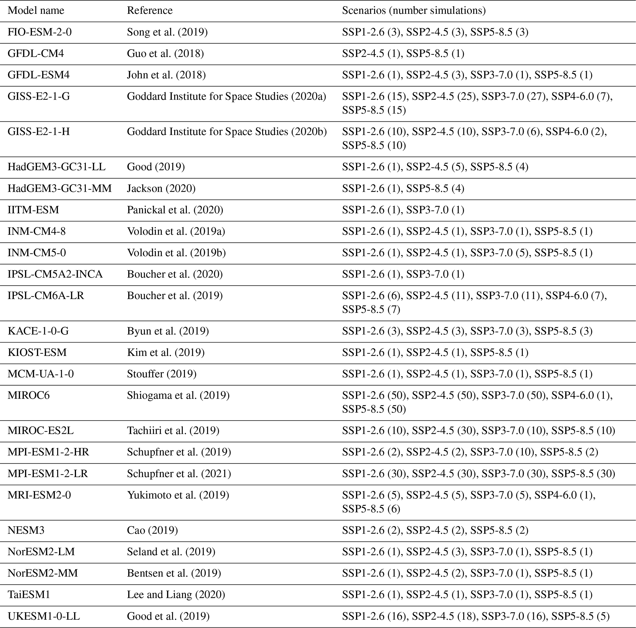
Table B1 Overview of the indicators shown in Sect. 2.4 and the variables, models, and simulations from the ISIMIP3 repository used as source data.

Appendix C: Additional validation plots

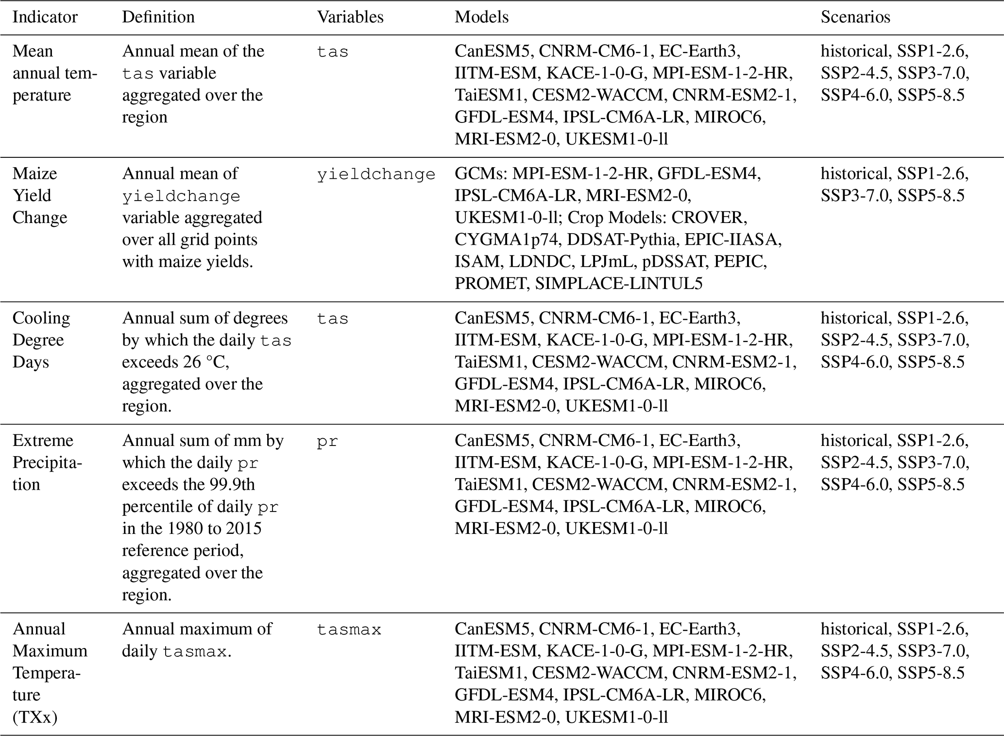
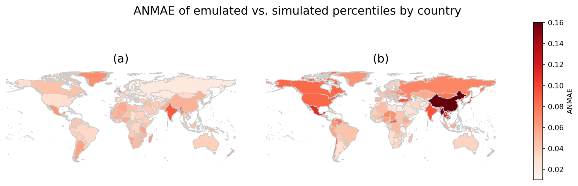
Figure C1 The average normalized mean absolute error (ANMAE, see Sect. 3.2.1) of emulated vs. simulated percentiles in each country. Panel (a) shows the annual average regional surface temperature compared to the 1995–2014 baseline for SSP1-2.6 in °C, and panel (b) shows the annual average regional precipitation compared to the 1995–2014 baseline for SSP1-2.6 in percent.

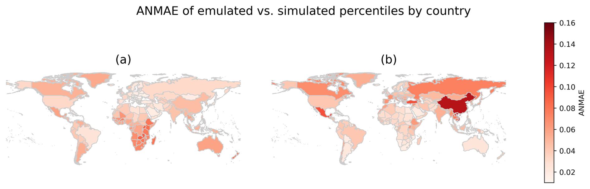
Figure C2 The average normalized mean absolute error (ANMAE, see Sect. 3.2.1) of emulated vs. simulated percentiles in each country. Panel (a) shows the annual average regional surface temperature compared to the 1995–2014 baseline for SSP3-7.0 in °C, and panel (b) shows the annual average regional precipitation compared to the 1995–2014 baseline for SSP3-7.0 in percent.

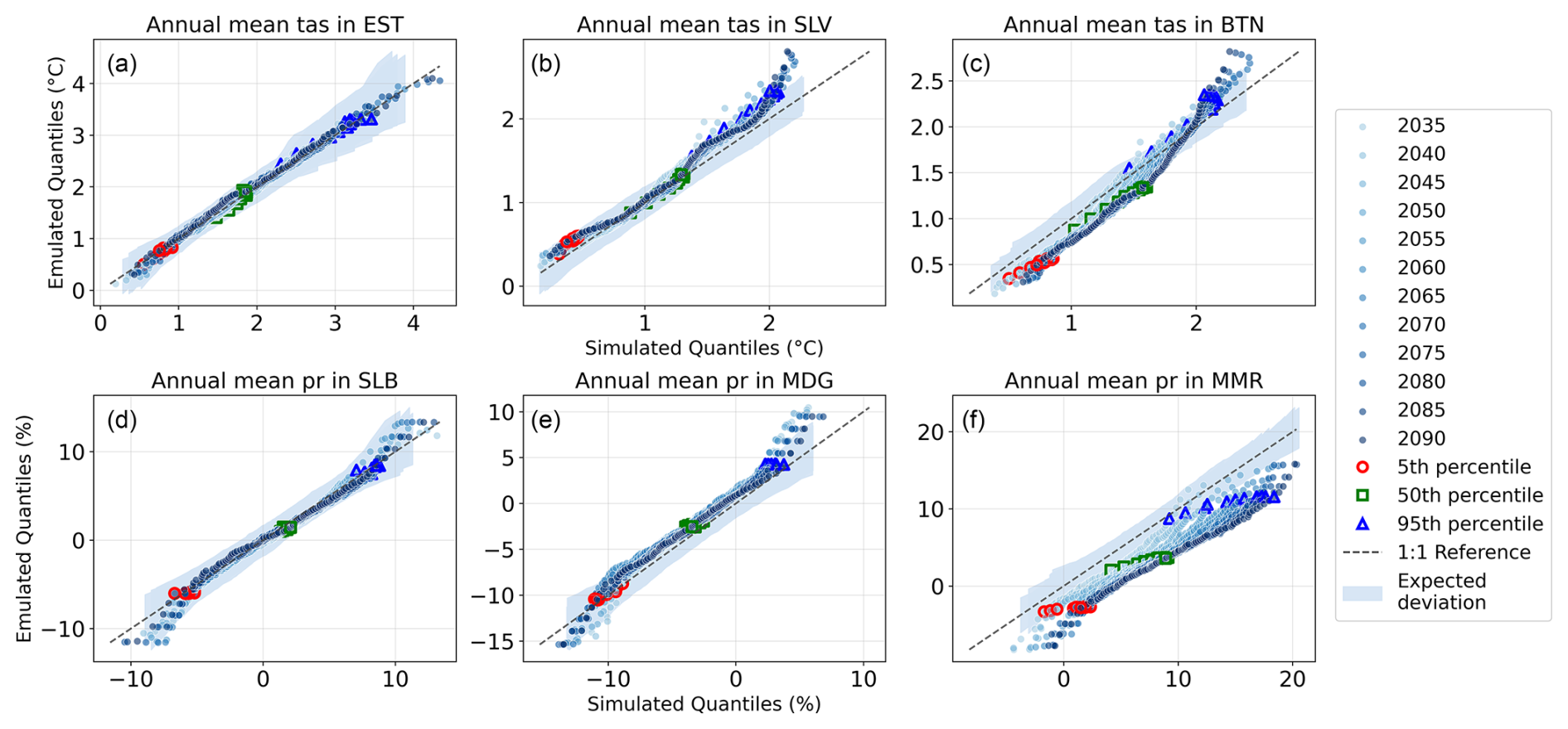
Figure C3 Q–Q plots showing the emulated and simulated percentiles from the CMIP6 ensemble. A perfect emulator and perfect knowledge of the simulated distribution would result in all points lying on the diagonal line included in the Q–Q plot. However, even if RIME-X were perfect, we would still expect a deviation of the emulated percentiles from the simulated percentiles as a result of the imperfect knowledge of the simulated distribution we have to estimate from around 150 samples. The expected deviation is quantified in the shaded area. While agreement across all percentiles is desirable, deviations in the tails are particularly important, as accurate representation of extremes is critical for many impact assessments. From left to right the examples illustrate the emulator performance for regions where the emulator showed the best, median, and worst performance as measured by the average normalized mean absolute error (ANMAE, see Sect. 3.2.1). In the first row we show the emulated and simulated percentiles of the annual average regional temperature (tas) compared to the 1995–2014 baseline in °C for selected regions, where (a) corresponds to Estonia (EST), (b) to El Salvador (SLV), and (c) to Bhutan (BTN). In the second row we show the emulated and simulated percentiles of the annual average regional precipitation change indicator (pr) in % for selected regions, where (d) corresponds to Solomon Islands (SLB), (e) to Madagascar (MDG), and (f) to the Myanmar (MMR).

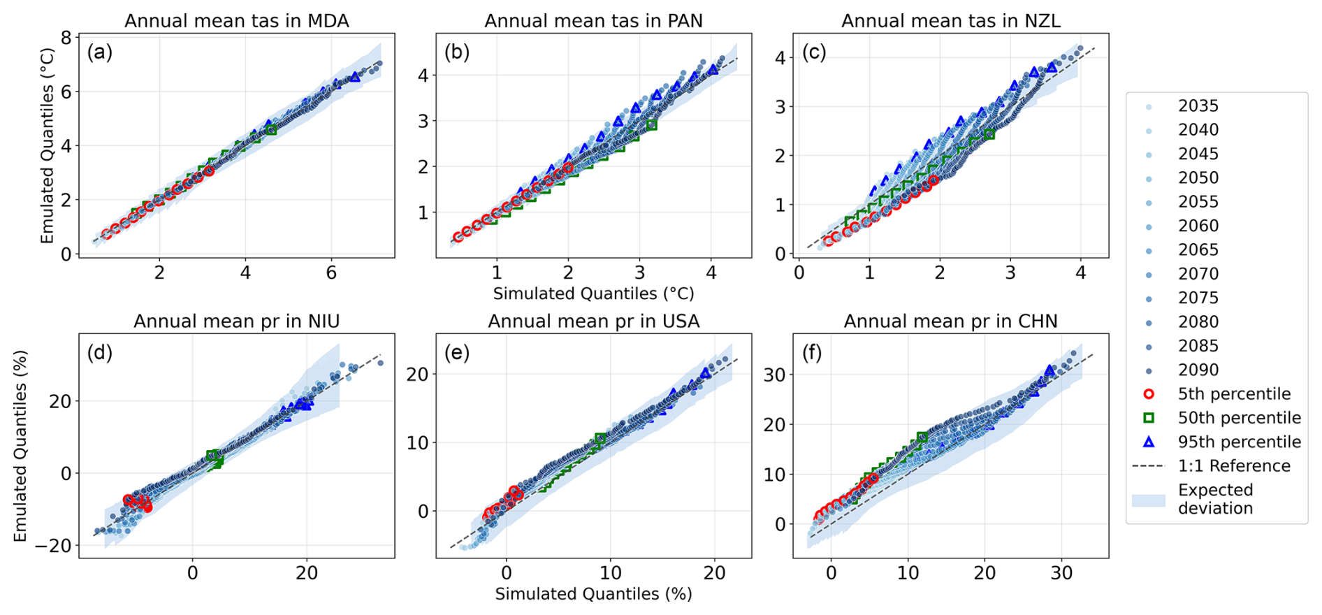
Figure C4 Q–Q plots showing the emulated and simulated percentiles from the CMIP6 ensemble. A perfect emulator and perfect knowledge of the simulated distribution would result in all points lying on the diagonal line included in the Q–Q plot. However, even if RIME-X were perfect, we would still expect a deviation of the emulated percentiles from the simulated percentiles as a result of the imperfect knowledge of the simulated distribution we have to estimate from around 150 samples. The expected deviation is quantified in the shaded area. While agreement across all percentiles is desirable, deviations in the tails are particularly important, as accurate representation of extremes is critical for many impact assessments. From left to right the examples illustrate the emulator performance for regions where the emulator showed the best, median, and worst performance as measured by the average normalized mean absolute error (ANMAE, see Sect. 3.2.1). In the first row we show the emulated and simulated percentiles of the annual average regional temperature (tas) compared to the 1995–2014 baseline in °C for selected regions, where (a) corresponds to Moldova (MDA), (b) to Panama (PAN), and (c) to New Zealand (NZL). In the second row we show the emulated and simulated percentiles of the annual average regional precipitation change indicator (pr) in % for selected regions, where (d) corresponds to Niue (NIU), (e) to United States of America (USA), and (f) to the China (CHN).

Appendix D: Validation of the RIME-X Emulator for Showcase Indicators

We provide an additional evaluation of the RIME-X emulator for the indicators presented in the Sect. 2.4. The evaluation compares the empirical median and 90 % confidence interval derived directly from the ISIMIP ensemble simulations for the SSP3-7.0 scenario with the corresponding emulated time series generated by RIME-X in five year steps from 2020 to 2090, based on all available ISIMIP simulations as training data and the GMT timeseries retrieved from the SSP3-7.0 ISIMIP simulations. We use the SSP3-7.0 scenario, because it represents the closest available primary ISIMIP scenario to the CAT Current Policies scenario used in the showcase in terms of its approximately linear warming trajectory, although with a stronger warming signal and different regional aerosol distribution. In addition, SSP3-7.0 provides complete coverage across all 14 ESMs and broad availability of agriculture-model simulations in case of the maize yield indicator. The evaluation Figs. D2 to D6 present results for 15 regions selected to represent the full range of emulator performance. For each of the 5th, 50th, and 95th percentile time series, we compute the average normalized mean absolute error (ANMAE; see Sect. 3.2.1) across all timesteps and select the regions nearest to the minimum, 5th percentile, median, 95th percentile, and maximum of the resulting error distribution. Figure D1 shows the ANMAE for each country and indicator. Some degree of discrepancy is expected because the empirical quantiles are estimated from only 14 ESM simulations, whereas the emulated quantiles are derived from all available simulations within the warming levels corresponding to the SSP3-7.0 trajectory for a given year. In particular, for extreme precipitation and for cooling degree days in Greenland (GRL), sampling uncertainty appears to account for a substantial share of the error. This is reflected in the relatively noisy empirical time series (Fig. D5 and the Greenland panel in Fig. D4). Despite this sampling uncertainty, the evaluation shows that RIME-X reproduces the main characteristics of the evolving distributions across indicators and regions. The ANMAE remains below 10 % in most cases and is often substantially lower (Fig. D1). The largest deviations occur for the 95th percentile of the maize yield indicator in the highest-error regions (Fig. D3). These discrepancies can largely be attributed to the impact model DSSAT-Pythia, which does not provide values in SSP3-7.0 but exhibits comparatively strong yield responses under SSP5-8.5 in the high-error regions North Korea (PRK), Liechtenstein (LIE), and Slovenia (SVN). As a result, these high values enter the RIME-X-derived distributions but are absent from the corresponding SSP3-7.0 reference ensemble, leading to inflated errors in the 95th percentile in these cases. Overall, maize yield change and extreme precipitation exhibit the highest error levels across indicators (Fig. D1). This is consistent with the known limitations of the RIME-X approach discussed in Sect. 3.1. In particular, extreme precipitation is, in addition to being sensitive to sampling uncertainty, strongly influenced by circulation changes, sea-surface-temperature-driven pattern effects, and monsoon dynamics, which may not be fully captured by a GMT-conditioned emulator. Similarly, maize yield changes depend not only on GMT but also on CO₂ concentration effects, which may introduce additional bias despite the strong correlation between GMT and CO₂ concentration in the scenarios considered.

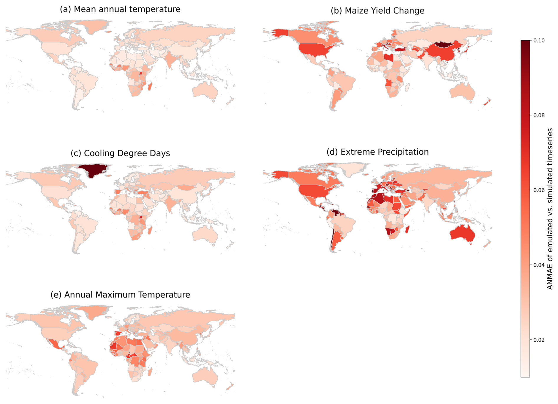
Figure D1 Error values comparing the 5th, 50th, and 95th percentile time series of mean annual temperature (a), maize yield change (b), cooling degree days (c), extreme precipitation (d), and annual maximum temperature (e). For each indicator, the 5th, 50th, and 95th percentile time series obtained from RIME-X emulations are evaluated against the corresponding empirical 5th, 50th, and 95th percentile time series directly computed from ISIMIP simulations for each country. Despite expected sampling uncertainty in the empirical percentiles, the average normalized mean absolute error (ANMAE) remains below 10 % in most cases and is often substantially lower, indicating strong agreement between emulated and simulated distributions.

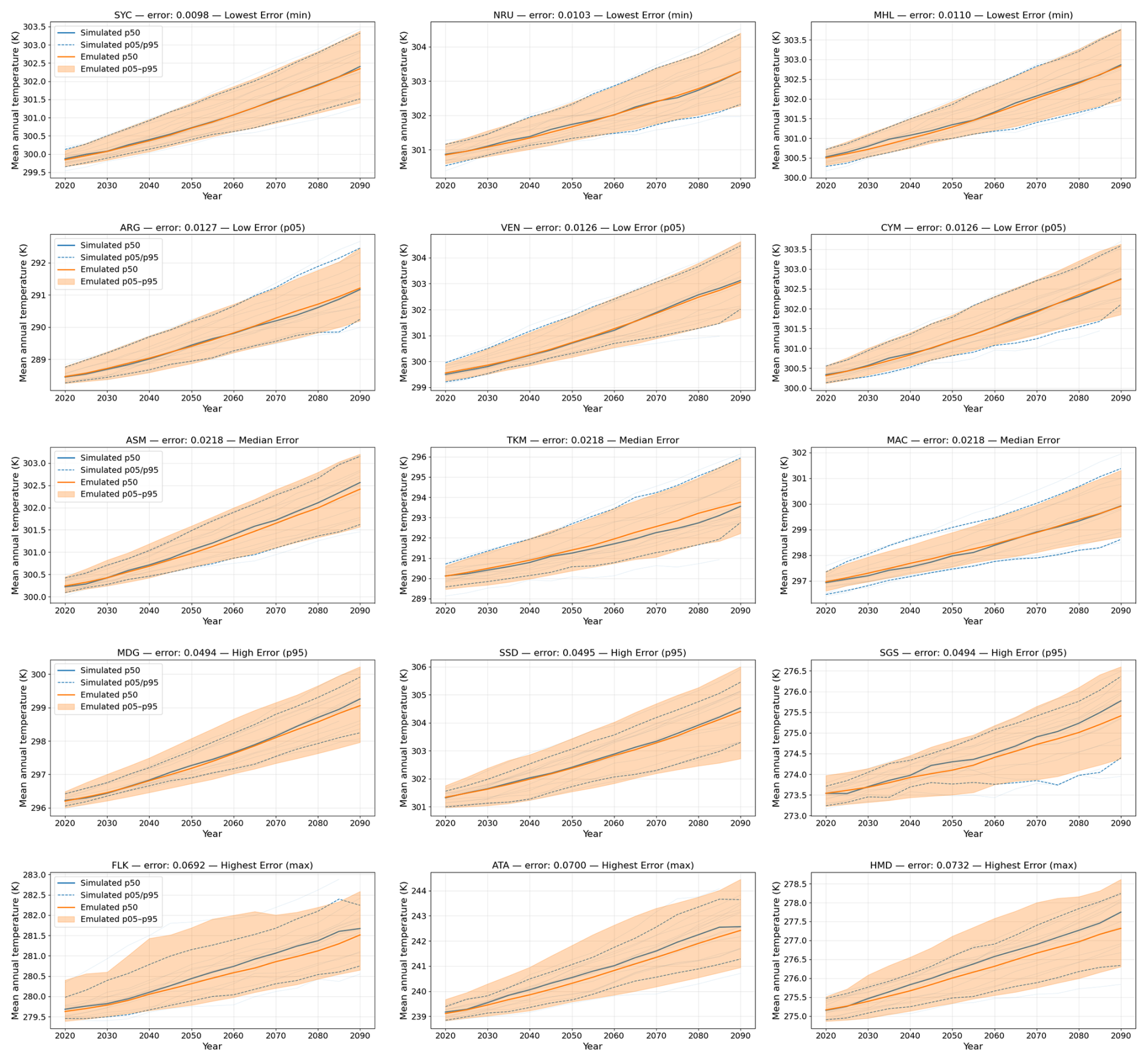
Figure D2 Time series of the 5th, 50th, and 95th percentile values of mean annual temperature (K) as emulated by RIME-X for the SSP3-7.0 scenario, compared to the corresponding empirical percentiles derived from ISIMIP simulations. The figure shows results for 15 selected regions: the three regions with the lowest, median, and highest normalized mean absolute error, as well as three regions each around the 5th and 95th percentiles of the error distribution.

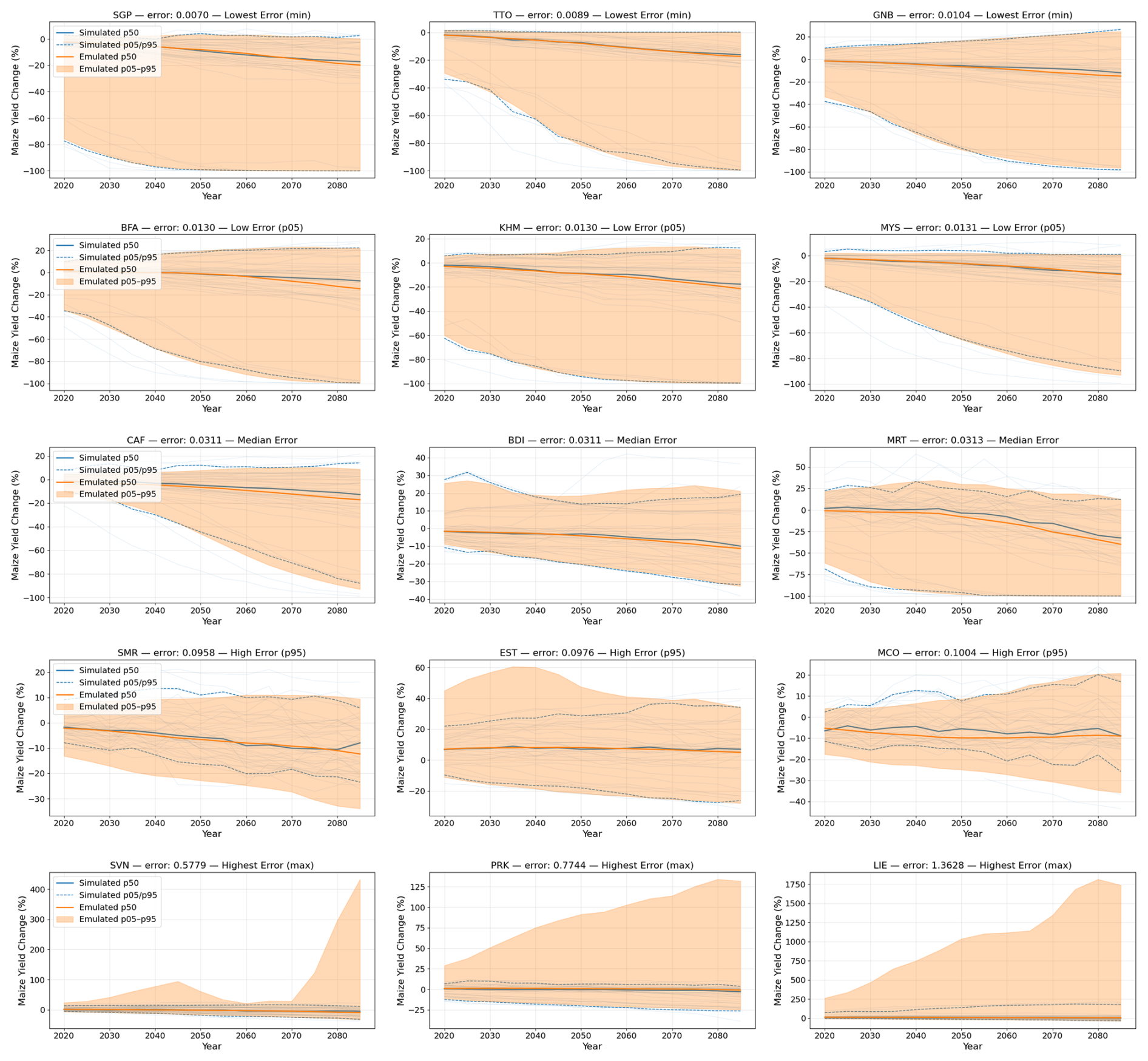
Figure D3 Time series of the 5th, 50th, and 95th percentile values of maize yield change (%) as emulated by RIME-X for the SSP3-7.0 scenario, compared to the corresponding empirical percentiles derived from ISIMIP simulations. The figure shows results for 15 selected regions: the three regions with the lowest, median, and highest normalized mean absolute error, as well as three regions each around the 5th and 95th percentiles of the error distribution. The particularly large maximum errors in the 95th percentile of this indicator can be traced to the impact model DSSAT-Pythia, which does not provide outputs for SSP3-7.0 but exhibits comparatively large values under SSP5-8.5. As a result, these values are included in the RIME-X-derived distributions but are absent from the corresponding “ground truth” SSP3-7.0 simulations, leading to inflated errors in the upper quantiles.

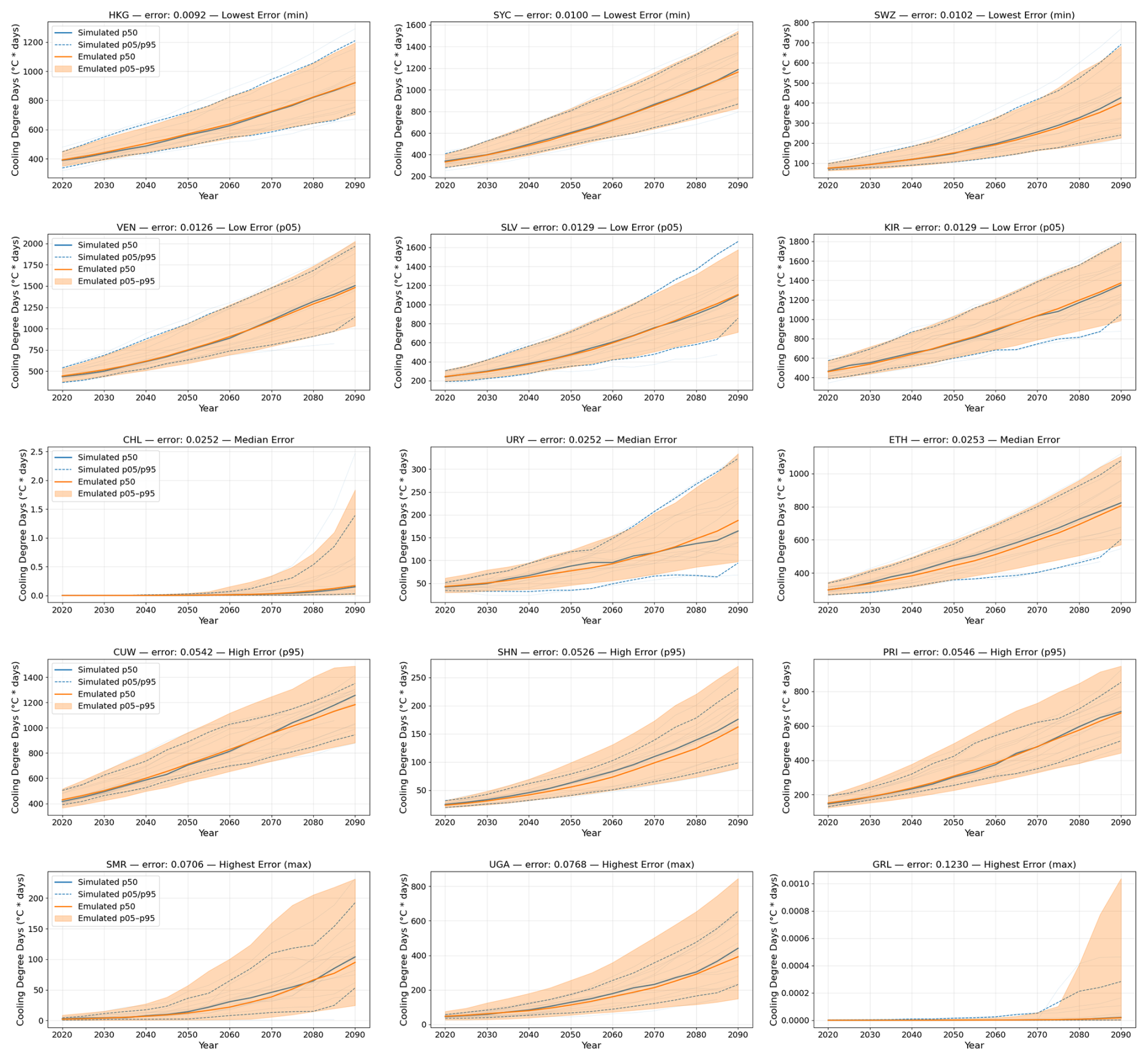
Figure D4 Time series of the 5th, 50th, and 95th percentile values of cooling degree days (°C ⋅ d) as emulated by RIME-X for the SSP3-7.0 scenario, compared to the corresponding empirical percentiles derived from ISIMIP simulations. The figure shows results for 15 selected regions: the three regions with the lowest, median, and highest normalized mean absolute error, as well as three regions each around the 5th and 95th percentiles of the error distribution.

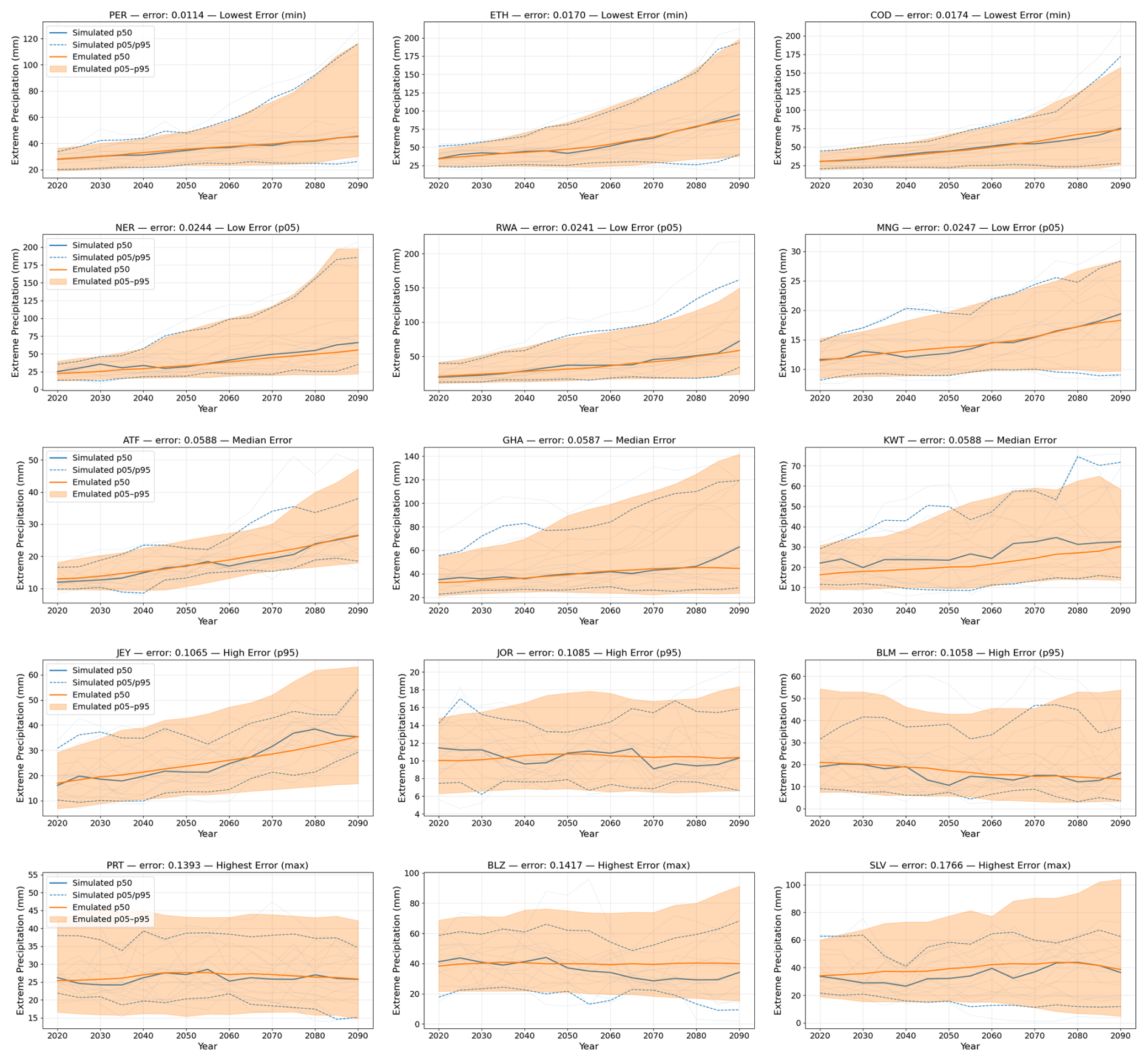
Figure D5 Time series of the 5th, 50th, and 95th percentile values of extreme precipitation (mm) as emulated by RIME-X for the SSP3-7.0 scenario, compared to the corresponding empirical percentiles derived from ISIMIP simulations. The figure shows results for 15 selected regions: the three regions with the lowest, median, and highest normalized mean absolute error, as well as three regions each around the 5th and 95th percentiles of the error distribution.

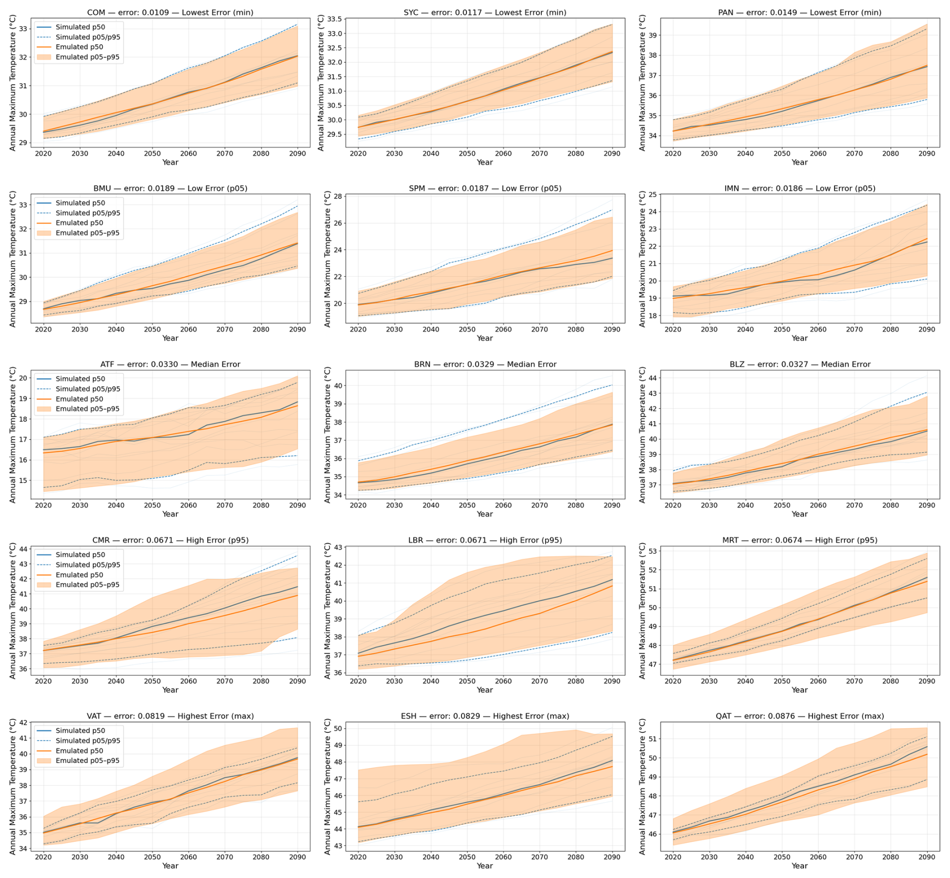
Figure D6 Time series of the 5th, 50th, and 95th percentile values of annual maximum temperature (°C) as emulated by RIME-X for the SSP3-7.0 scenario, compared to the corresponding empirical percentiles derived from ISIMIP simulations. The figure shows results for 15 selected regions: the three regions with the lowest, median, and highest normalized mean absolute error, as well as three regions each around the 5th and 95th percentiles of the error distribution.