Computational library for the nutrient-unicellular-multicellular plankton modeling framework v. 1.0

The nutrient-unicellular-multicellular (NUM) model is a trait-based model of unicellular and multicellular plankton that uses body size as the main structuring variable for community composition. The central feature is that body size is used for structuring predator-prey interactions and to scale parameters. For unicellular plankton, trophic strategies across the full range from osmotrophy, phototrophy, phagotrophy, and mixotrophy are an emergent outcome of the model. Another distinguishing feature is that the multicellular component, represented by copepods, includes ontogeny, which is crucial in shaping population dynamics. In addition, the framework encompasses a nutrient pool consisting of nitrogen, silica and dissolved organic carbon (DOC) which interacts dynamically with the plankton community in three model setups: a chemostat simulating the photic zone, a water-column, and a global setup. Here we present a user-friendly Fortran-Matlab library which makes the NUM model accessible as a practical tool for marine ecologists or biogeochemical modellers. The model output is validated with in situ and satellite data and demonstrates its applicability in chemostat, water-column, and global setups.

1 Introduction

Marine planktonic food webs play an important role in the ocean's biogeochemical cycles, influence the Earth's climate regulation, and determine potential fisheries yields (Stock et al., 2014). Plankton participate in the global carbon cycle by accounting for roughly half the global carbon fixation through photosynthesis, and by sequestering carbon via sinking dead detrital matter (Basu and Mackey, 2018; Boyd et al., 2019). The production of new biomass from photosynthesis also determines the amount of carbon available to higher trophic levels of fish production, which globally support about 17 % of human protein consumption (Waite et al., 2014).

The central problem that ecosystem models face is how to represent the immense diversity of species in a tractable yet mechanistically meaningful way. The dominant approach has been to assemble similar kinds of species into functional groups. In the simplest formulation, the planktonic community is divided into phytoplankton and zooplankton in “NPZ” models (Franks, 2002). A finer representation of diversity is introduced by subdividing plankton into functional types (Le Quéré et al., 2005) e.g., flagellates, dinoflagellates, ciliates, and diatoms (Butenschön et al., 2016), or into size groups, e.g., small- and large phytoplankton (Neumann, 2000) or sizes of zooplankton (Stock et al., 2014). The addition of each functional group fills another piece in the puzzle towards a complete representation of plankton diversity, however, it also brings a new set of parameters, which must be specified. The expanded set of parameters lends flexibility because the parameters for each functional group can be calibrated to reflect the dominant species in a particular region (Turner et al., 2014). While such calibrations make it possible to achieve good fits with observations, for global applications or for applications of environmental change, where the dominant species may change, the calibration may be driven outside its calibration envelope. Nevertheless, the functional group approach represents a robust solution to the representation of diversity that also retains a direct connection to the taxonomic representation of life.

An alternative approach has been to represent plankton diversity solely through differences in their size (cell size or body size) (e.g. Ward and Follows, 2016; Chakraborty et al., 2020; Andersen and Visser, 2023; Hansen et al., 2025). Using only size to represent diversity eschews any representation of taxonomic diversity, even down to not distinguishing between phyto- and zooplankton. Practically, body size is discretized in a number of size groups with an ordinary differential equation to represent each size group. Although size-based models may well have the same number of state variables as functional-type models, they have only one set of parameters that applies across all groups through scaling relations (Andersen et al., 2016). However, while size is indeed recognized as the “master” trait, pure size-based representations ignore key functional groups such as diatoms (Cadier et al., 2020), bacteria, or obligate phytoplankton and zooplankton. In practice plankton models often adopt a mixture of size-based and functional-group type of models, e.g., using size for diversity inside functional groups of phyto- and/or zooplankton (Banas, 2011; Stock et al., 2014; Ward et al., 2014, 2018), or diatoms (Terseleer et al., 2014). This method enables functional-group type of models to reduce their parameter set through scaling relations with size.

The approach followed here is to represent diversity through functional traits (Kiørboe et al., 2018). In the idealized case, a trait-based approach ignores all taxonomical differences between organisms and only describes differences between organisms through a small set of functional traits (Westoby and Wright, 2006). A trait-based representation of diversity requires a decision about which trait-axes to model, i.e., which traits are most important for the functional diversity of the community. While there is wide agreement about cell or body size as the master trait, various other trait axes have been proposed for the secondary axes, such as investments into resource uptakes: phototrophy and nutrient harvesting (Bruggeman and Bolding, 2014) or including also phagotrophy (Berge et al., 2017; Chakraborty et al., 2017, 2020), degree of gelatinousness (Lemoine et al., 2025), feeding mode (active vs. passive) (Prowe et al., 2019; Serra-Pompei et al., 2020), or vacuolation (Cadier et al., 2020). When traits are discrete, as for active/passive feeding or for unicellular plankton with or without a silicate shell, the trait-based representation becomes essentially identical to the functional type approach. In that respect the differences between the two approaches are mainly conceptual – whether the representation of diversity is oriented towards taxonomical differences or functional traits.

Here we present an implementation of the trait-based nutrient-unicellular-multicellular (NUM) plankton model framework (Serra-Pompei et al., 2020). The NUM framework attempts to make a pure trait-based plankton model. It uses cell size as the primary trait for unicellular plankton and silicate shell as a discrete trait (essentially a diatom functional group). For multicellular plankton it uses adult size as the primary trait and active/passive feeding mode as a secondary discrete trait. The NUM framework focuses on the ecology of the plankton and puts less focus on the chemistry. It therefore only includes a very basic representation of nutrient chemistry.

A distinguishing feature of the NUM model is a representation of multicellular plankton which explicitly resolves the developmental stages of copepods. Such representations remain rare (but see Record et al., 2013) for two reasons: first, multicellular zooplankton can increase by several orders of magnitude in body mass from eggs to adults, with a growth rate which depends on the availability of food, among other factors. Representing multiple stages requires several state variables to represent just one species. Second, copepod diversity varies strikingly in different regions (Rombouts et al., 2009) and representing all dominant species in global models is not feasible. The nutrient-unicellular-multicellular (NUM) model solves the first problem by using an efficient representation of life history as a physiologically structured model (De Roos et al., 2008) and the latter problem by describing the diversity of copepods by two traits: their adult body size and their feeding mode (passive or active) (Serra-Pompei et al., 2020).

A central ambition of the NUM model is to base all parameters on “first principles”, thereby avoiding free parameters that require calibration. The first principles can be related directly to physical laws (diffusion, fluid mechanics, etc.), energetics of chemical reactions, geometry, or mass conservation. This ambition is realized for many of the parameters for the unicellular compartment (Andersen and Visser, 2023). The challenges increase for the multicellular compartment, and here most parameters are determined by cross-species analyses. The description of the parameter values is reported elsewhere (Serra-Pompei et al., 2020; Cadier et al., 2020; Hansen and Visser, 2019; Andersen and Visser, 2023) and the focus here is on the implementation of the NUM framework as a computational platform for plankton ecology on a global scale.

A technical difficulty concerns the reduction of computational time for executing global simulations of full plankton ecosystem models. To provide marine ecologists without expertise in global biogeochemical modelling the ability to perform global simulations we based the global simulations on the transport matrix method (Khatiwala, 2007). The NUM model library version 1.0 is based on the NUM model as described in Serra‐Pompei et al. (2022) with a number of key additions: (1) the inclusion of an explicit diatom functional group and silicate dynamics; (2) inclusion of labile dissolved organic carbon and (emergent) heterotrophic bacteria; (3) emergent respiration of unicellular plankton due to uptake regulation; (4) a fast Fortran implementation of the core functions; (5) a matlab front-end interface with three model setups: chemostat, water column, and global; (6) a flexible configuration of plankton communities, ranging from a single-celled group (e.g. unicellular generalists, including osmotrophs, phototrophs, phagotrophs, and mixotrophs) to a full setup with unicellular generalists, diatoms, sinking particulate organic matter, and a complete representation of the multicellular copepod community.

In the following, we first provide an overview of the NUM model structure and implementation, followed by a description of the key equations in the model. Next, we compile global calibration and validation data and compare it with global model simulations. Finally, we present examples of the model output, from global patterns to cell-level metabolism, and discuss open issues and potential applications of the NUM library.

2 The nutrient-unicellular-multicellular library version 1.0

The core NUM model consists of a set of coupled ordinary differential equations for the state variables. These equations are all coded in a Fortran library for computational efficiency, while the code is executed from a matlab interface. The equations require a representation of the physical environment, which could be a global or regional circulation model or a simple chemostat (Andersen and Visser, 2023). The matlab front-end to the Fortran library interfaces with three environments: a chemostat, a water-column, and the entire globe. All the setups are derived from a global transport matrix that represents a discretized version of the underlying geophysical partial differential transport equations (Fig. 1a). The combination of computationally efficient compiled code with an interpreted language allows to run global simulations on a standard laptop.

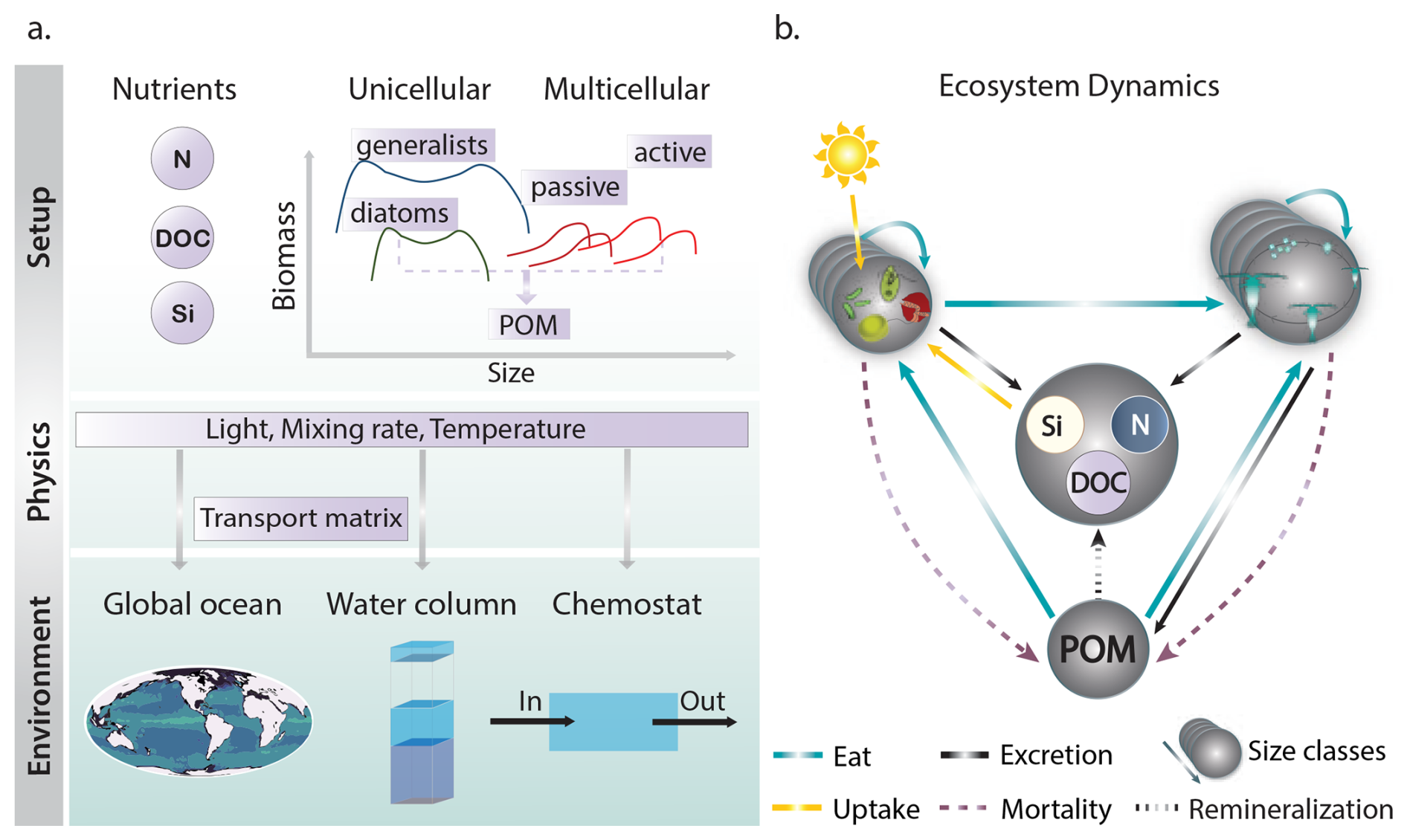
Figure 1 Conceptual sketch of the NUM framework. Panel (a) illustrates the ecological setup and the coupling to physical environments. Panel (b) describes the ecosystem dynamics. Several size-classes are modeled in each plankton group. The number of size classes and plankton groups can be defined at the beginning of each model run.

The NUM state variables belong to one of three groups: biogeochemical tracers (referred to as “nutrients”, including dissolved organic carbon DOC, nitrogen, and silicate), unicellular plankton (generalists or diatoms), multicellular zooplankton groups (copepods), and particulate organic matter (POM) (Fig. 1b). The three nutrient variables are the minimal set needed to represent growth limitation for phytoplankton (incl. diatoms which are limited by silicate) and the carbon source for osmoheterotrophs (bacteria). The unicellular and multicellular groups are represented by “size spectra” encompassing a number of state variables that each models the dynamics of one size group (Fig. 1a). By implementing several sizes of the unicellular and multicellular groups, the size spectrum of the entire plankton community emerges. Size – defined as cell mass of unicellular organisms and body mass of multicellular organisms – is the key trait that describes resource encounter and uptake, as well as the physiology of individual plankton organisms (metabolism, growth, and reproduction) (Hillebrand et al., 2022). Further, size determines the central process in the model, which is predation by larger organisms on smaller ones (Wirtz, 2012). By using size as the core structuring variable, each organism group is described by one set of parameters defined through size scalings. This approach reduces the overall number of parameters and permits a flexible number of state variables.

The four size spectrum groups described below are generalists, diatoms, copepods, and dead particulate organic matter (POM).

2.1 Unicellular generalists

The “generalist” group represents all unicellular plankton including bacteria, phytoplankton, phagotrophs, and mixotrophs (organisms which combine trophic strategies, such as photosynthesis, diffusive uptake of nutrients and predation on smaller cells), but excluding diatoms. This group therefore encompasses a wide range of unicellular organisms, such as heterotrophic and photosynthetic bacteria, flagellates, dinoflagellates, and ciliates, while diatoms are simulated as a separate group (explained in the following section). The generalists are all modeled as potential mixotrophs that acquire carbon and nutrients through a combination of osmotrophy (taking up dissolved organic carbon), autotrophy (photosynthesis), and/or phagotrophy. Whether a given size group represents bacteria, phytoplankton, etc., depends on the principal mode of carbon acquisition, which is determined by a combination of cell size and the environment. The trophic strategies of each size class are therefore an emergent property and vary dynamically over space and time. The generalist spectrum is thus a trait-based model with cell size being the trait.

2.2 Diatoms

Large diatoms, that thrive in eutrophic environments, have historically been correlated with food webs that lead to major fisheries (Ryther, 1969). Thus, the inclusion of diatoms in the model is critical for the estimation of fish production potential. Diatoms are simulated as a separate group because of their importance in marine systems (they account for about 40 % of marine primary production (Tréguer et al., 2018)), and their distinct characteristics that affect their physiology and predation mortality. Diatoms enclose a vacuole that increases their volume, allowing them to have larger physical size than other cells of the same biomass. In the model, this trait allows them to increase their volume per carbon without additional nutrient demands allowing them to have a higher per-carbon diffusive uptake than non-vacuolated cells. Further, diatoms are engulfed in a silicate shell, which makes silicate another limiting nutrient. The hard silica shell also reduces predation pressure on the diatoms (Hamm et al., 2003; Pančić et al., 2019). The rigidity of the hard silica shell deprives the cell of the plasticity needed to engulf prey and excludes diatoms from eating prey. Diatoms therefore cannot perform phagotrophy and only obtain nutrients through diffusive uptake. The silicate shell also induces growth limitation of diatoms by dissolved Si, besides light and nitrogen.

2.3 Copepods

Multicellular zooplankton are the key link between lower and higher trophic levels, as they ingest unicellular plankton and are themselves prey for fish. Among the different zooplankton taxa in the ocean, copepods are the most abundant metazoans (Humes, 1994). Copepods undergo size changes throughout their life stages and thereby occupy different ecological niches. These ontogenetic niche shifts substantially impact population dynamics (Verity and Smetacek, 1996). For instance, copepod growth rates are strongly correlated with spring bloom intensity (Durbin and Durbin, 1992). To account for these size changes, each population of copepods is represented by a size spectrum that spans from the offspring size to the adult size.

Each population of copepods is characterized by two traits: the adult size and their feeding strategy (active or passive). In this way, the model represents the large differences in adult size observed in the oceans (Brun et al., 2016). Modelling the diversity of copepods with these two main traits makes it possible to represent the entire copepod community in the global ocean with just a few populations that span the trait space of adult size and feeding modes.

2.4 Particulate organic matter

Dead organic matter (detritus) is represented by a size spectrum of particulate organic matter (POM) that includes dead organisms, cell fragments from lysis, and fecal pellets produced by multicellular plankton. POM may be represented by a size spectrum to enable the calculation of sinking velocities for different POM sizes. However, in the simulations presented here we simulated just a single size class of POM.

3 Model description

Here we describe the main processes in the NUM model. We first describe the size-based predation among modeled organisms and by larger “higher trophic level” (HTL) organisms that are not represented by the model. Then we describe the cell model (generalists and diatoms), the multicellular model, the POM model, and the biogeochemical model (Fig. 1). The full equations for each model component are listed in Appendix B.

3.1 Predation

Predation is the central process that connects the plankton size classes in NUM. Each size class i is characterized by its mass m_i (either cell mass or body mass in µg carbon) and the organisms in the class prey on smaller organisms m_prey with a log-normal preference function:

$$\begin{array}{}\text{(1)}& {\mathit{\varphi }}_{kl}\left(m,m_{\mathrm{prey}}\right)=p_{kl}\exp \left[-{\displaystyle \frac{\mathrm{1}}{\mathrm{2}{\mathit{\sigma }}_k^{\mathrm{2}}}}{\left(\ln \left({\displaystyle \frac{m}{{\mathit{\beta }}_k{m}_{\mathrm{prey}}}}\right)\right)}^{\mathrm{2}}\right],\end{array}$$

where β is the preferred predator:prey mass ratio, σ is the width, and p_kl is the preference of the predator group, i.e. copepods, k towards the prey group l, i.e., diatoms (all parameters are specified in Tables B2, B4, and B5 in the supplementary). As each size class represents a finite range of sizes (with m representing the geometric mean; see Fig. A1), the actual preference is the average of the encounter over all prey and predator masses, so the average encounter θ_ij between two size classes i (predator) and j (prey) becomes a more complex function (Appendix C).

The available food for size class i is the sum over all other size classes weighted by the preference (θ_ij): $F_i=\sum _j{\mathit{\theta }}_{ij}{B}_j$ where B_j is the biomass concentration of prey (µg C L⁻¹). The actual consumption is limited by a mass-specific maximum consumption rate: j_Fmax (d⁻¹):

$$\begin{array}{}\text{(2)}& j_{\mathrm{F}.i}={\mathit{ϵ}}_{\mathrm{F}}{f}_i{j}_{\mathrm{Fmax}.i}\mathrm{with}{f}_i={\displaystyle \frac{a_{\mathrm{F}.i}{F}_i}{a_{\mathrm{F}.i}{F}_i+j_{\mathrm{Fmax}.i}}},\end{array}$$

where a_F.i is the mass-specific clearance rate of the predator (L(µg C d)⁻¹) and ϵ_F is the assimilation efficiency. The predation results in a predation mortality on the prey size class j:

$$\begin{array}{}\text{(3)}& {\mathit{\mu }}_{\mathrm{pr}.j}=\sum _i{\mathit{\theta }}_{ij}{\displaystyle \frac{j_{\mathrm{F}.i}{B}_i}{{\mathit{ϵ}}_{\mathrm{F}}{F}_i}}.\end{array}$$

In addition to the predation mortality inflicted by larger plankton, the largest size classes are also exposed to predation by higher trophic levels that are not explicitly represented in the model, such as fish. The exposed size classes are those larger than m_HTL (µg C), described by the selectivity function p_HTL:

$$\begin{array}{}\text{(4)}& p_{\mathrm{HTL},i}={\displaystyle \frac{\mathrm{1}}{\mathrm{1}+{\left(m_i/m_{\mathrm{HTL}}\right)}^{-\mathrm{2}}}}.\end{array}$$

Here we use a value of the m_HTL=1 µg C (≈500 µm) as the size of prey of forage fish in the size range 1–10 g wet weight (Andersen, 2019, Chap. 2). Further, in the standard setup presented here, we constrain the higher trophic level (HTL) mortality to act only on copepods. If a setup is run without copepods the HTL mortality would represent the predation by the copepods on the unicellular organisms. The higher trophic level mortality can either be a constant or proportional to the biomass concentration in the size class:

$$\begin{array}{}\text{(5)}& {\mathit{\mu }}_{\mathrm{HTL},i}=\left\{\begin{array}{ll}{\mathit{\mu }}_{\mathrm{HTL},\mathrm{0}}{p}_{\mathrm{HTL},i}& \mathrm{constant}\\ {\mathit{\mu }}_{\mathrm{HTL},\mathrm{0}}{p}_{\mathrm{HTL},i}\frac{B_i}{\ln \left(\mathrm{1}/z_i\right)}& \mathrm{`}\mathrm{`}\mathrm{quadratic}\text{”}\end{array}\right..\end{array}$$

The density dependent mortality is termed “quadratic” to follow common nomenclature, though the mortality is in reality linear and it is only the loss term (mortality multiplied by biomass) that is quadratic. The quadratic formulation of mortality has the practical advantage that it helps stabilize the dynamics in the simulation – running without a quadratic loss term results in competitive exclusion among copepod groups and limited co-existence. We therefore use the quadratic mortality formulation in this capacity. The term $\mathrm{1}/\ln (\mathrm{1}/z_i)$ is a correction for the number of size classes used. Size classes are evenly distributed on a logarithmic size grid and in that case the number of size classes in a fixed size range is proportional to this correction term, where z_i is the ratio between the lower and the upper size range in each size class. It should be noted that higher trophic level mortality does not respect the increased prey vulnerability due to motility that predation mortality follows. This assumption follows from higher trophic level organisms being visual predators and the hydrodynamic signals from prey motility do not affect the detection of prey (Howe et al., 2018; Lange Jensen et al., 2023).

3.2 Cell model

The unicellular spectra can be either generalists or diatoms. The only differences between the two spectra are that diatoms have a vacuole, that they cannot perform phagotrophy, and that they have a lowered predation risk (p<1) (as explained above). The present description of diatoms with a fixed vacuole size is a simplified version of the description with dynamic vacuoles in Hansen and Visser (2019); Cadier et al. (2020). The full set of equations and parameters for the unicellular model are given in Tables B1 and B2.

The cell model describes the encounter and uptake of resources and metabolism of an individual plankton cell as modulated by the cell's size (mass) m (µg C). The size of the cell defines traits, and traits in combination with the environment define its trophic strategy, whether it is an osmo-heterotroph (a bacterium feeding mainly on DOC), a light- or nutrient-limited phototroph, or, for the generalists, a mixotroph (combining osmo-, photo-, and phagotrophy) or a heterotroph (living mainly on phagotrophy) (Andersen et al., 2016).

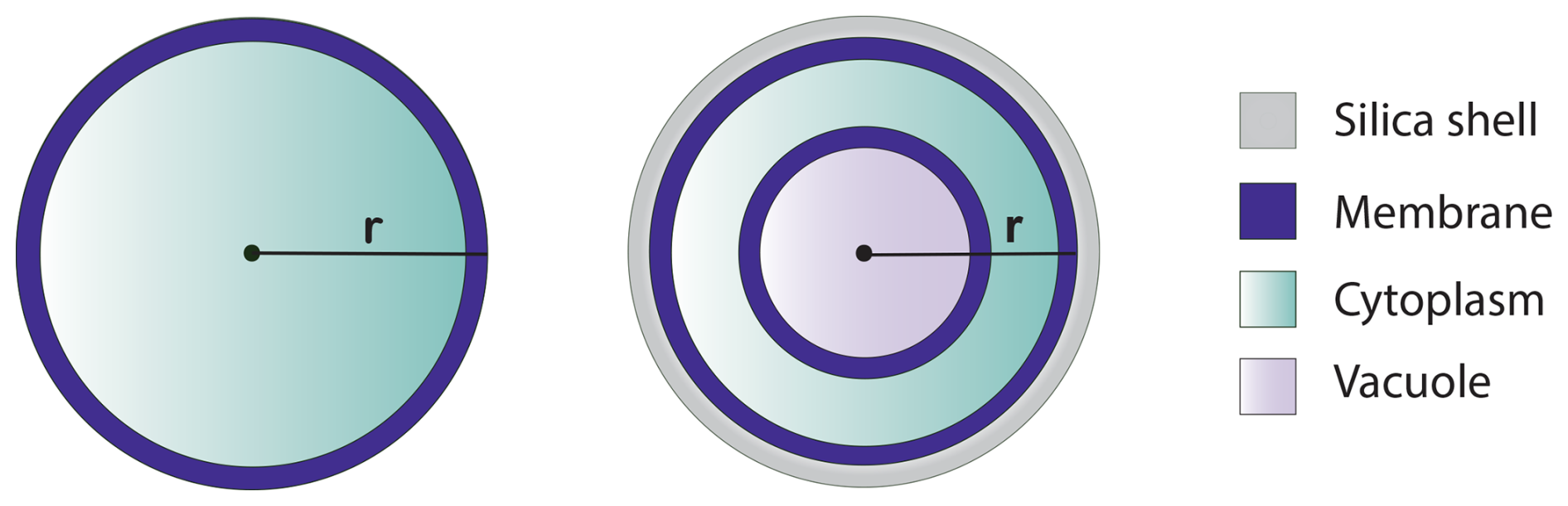
Regarding their morphology, we assume that cells are spherical and consist of a cytoplasm surrounded by a membrane of thickness δ (Fig. 2). The diatom cells additionally have a vacuole that occupies a fraction v_vac of the cell volume and is surrounded by an additional inner membrane. The radius of a cell with mass m is approximately (assuming δ≪r) (Eq. B5):

$$\begin{array}{}\text{(6)}& r={\left({\displaystyle \frac{\mathrm{3}}{\mathrm{4}\mathit{\pi }}}{\displaystyle \frac{m}{\mathit{\rho }}}{\displaystyle \frac{\mathrm{1}}{\mathrm{1}-v_{\mathrm{vac}}}}\right)}^{\mathrm{1}/\mathrm{3}},\end{array}$$

where ρ is the density of the cytoplasm (µg C µm⁻³). A fraction ν of the cell's mass is used for the membrane(s), and the remainder 1−ν is mass available for active metabolism. The fraction of the cell mass that is membranes for a generalist cell is (Andersen and Visser, 2023):

$$\begin{array}{}\text{(7)}& \mathit{\nu }=\mathrm{3}{\displaystyle \frac{\mathit{\delta }}{r}},\end{array}$$

and for a diatom given in Eq. (B6). The cell model describes three processes: encounter with resources, uptake of resources and metabolism, and mortality.

Figure 2 Geometry of generalist and diatom cells.

3.2.1 Encounter

The cell takes up carbon via photosynthesis (light), while both carbon and nitrogen are taken up via phagotrophy (i.e. eating prey; only generalists) and diffusion, in the form of dissolved organic carbon (DOC) and dissolved inorganic nutrients respectively (Fig. 3). Diatoms also take up silicate to build their silica shell. The encounter with the resources (light L, DOC, N, prey F, and silicate Si) is described as specific mass fluxes j_X (d⁻¹):

$$\begin{array}{}\text{(8)}& j_{\mathrm{enc}.X}=a_X\left(m\right)X{\mathit{\rho }}_{\mathrm{C}:X},\mathrm{with}X\in \mathit{\{}\mathrm{DOC},\mathrm{N},\mathrm{L},\mathrm{F},\mathrm{Si}\mathit{\}}\end{array}$$

where ρ_C:X is the ratio between carbon and the element of the resource X and a_X is the mass specific affinity.

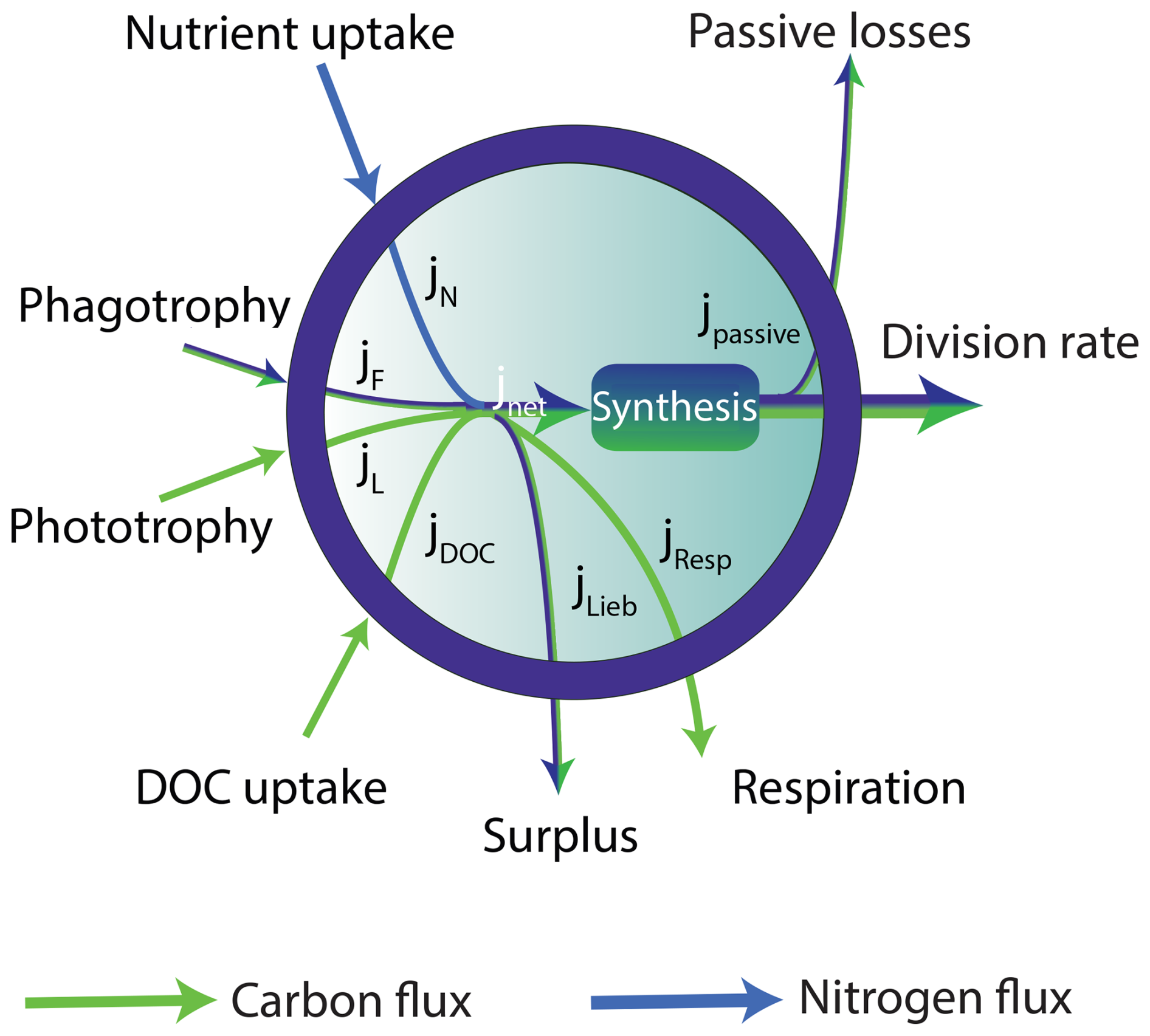
Figure 3 Illustration of the cell metabolism of a generalist with uptakes of resources as carbon (blue arrows) and nutrients (green arrows), losses due to respiration or passive losses, biosynthesis leading to cell division rate g, resulting in a net division rate. The diatom cell is similar, but with an additional uptake of silicate j_Si and no phagotrophic uptake.

The affinity for each resource uptake is determined by the geometric properties of the cell and is expressed as a function of mass (m) and the radius r. The dependency of affinities on size is analysed comprehensively in Andersen and Visser (2023) and given in Table B1. Generally, the diffusive uptake is limited by the cell radius, light uptake by the cell cross-sectional area, and feeding by the cell volume.

3.2.2 Metabolism

The cell division rate depends on light and available resources. The uptake of resource X has a metabolic carbon cost β_Xj_X. The cell has different sources of both carbon and nutrients; carbon from photosynthesis, DOC, and food, and nutrients from dissolved N and food, each with different metabolic costs of uptake. The cell regulates the uptakes j_X of the encountered resources j_enc.X down towards the effective uptakes j_net in order to maximize division rate under the constraint of a fixed C : N : Si stoichiometry (Liebig's law of the minimum) (Table B1 “resource uptakes”). The regulation of light absorption acts as a simple representation of light-adaptation, while the regulation of the nutrient uptakes represent Liebig's law. The emergent respiration is:

$$\begin{array}{}\text{(9)}& j_{\mathrm{resp}}=j_{\mathrm{R}}+\sum _X{\mathit{\beta }}_X{j}_X+{\mathit{\beta }}_{\mathrm{g}}g,\end{array}$$

where j_R is the basal metabolism and β_gg is the growth metabolism as a fraction of the division rate g. The cell division rate is limited by its capacity for biosynthesis j_max (Eq. B1.15):

$$\begin{array}{}\text{(10)}& g=j_{\max }{\displaystyle \frac{j_{\mathrm{net}}}{j_{\mathrm{net}}+j_{\max }}}-j_{\mathrm{passive}},\end{array}$$

where j_max is proportional to the active cell mass v (Eq. 7), and j_passive are passive losses across the cell surface.

3.2.3 Population growth

Besides predation losses (Eqs. 3 and 5) the cell is exposed to viral lysis with a mortality μ₂ proportional to the cell biomass:

$$\begin{array}{}\text{(11)}& {\mathit{\mu }}_{\mathrm{2}.i}={\mathit{\mu }}_{\mathrm{2}}{B}_i/\ln \left(\mathrm{\Delta }{m}_i\right)\end{array}$$

where Δm_i is the width of the size class (Fig. A1). The correction with the width of the size class is needed because the biomass B_i describes the biomass in a size class i, and the biomass will vary depending on the width of the size class (increasing the size range (width) of a size class by a factor increases the biomass in the bin by the same factor).

The final growth equation for the unicellular plankton is:

$$\begin{array}{}\text{(12)}& {\displaystyle \frac{\mathrm{d}{B}_i}{\mathrm{d}t}}=\left(g_i-{\mathit{\mu }}_{\mathrm{pr},i}-{\mathit{\mu }}_{\mathrm{HTL},i}-{\mathit{\mu }}_{\mathrm{2},i}\right)B_i,i\in \mathrm{uni}\end{array}$$

where uni = {all unicellular groups}.

3.3 Multicellular model

Copepods represent multicellular zooplankton and the copepod community consists of different populations. Each population is characterized by the adult body-mass and the feeding mode (active or passive). The spectrum for the population resolves the life stages of copepods, from nauplii to adults, following the description in Serra-Pompei et al. (2020):

$$\begin{array}{}\text{(13)}& \begin{array}{rl}{\displaystyle \frac{\mathrm{d}{B}_i}{\mathrm{d}t}}=& J_{\mathrm{in},i}+\left(j_{\mathrm{out}.i}+g_i-{\mathit{\mu }}_{\mathrm{pr}.i}-{\mathit{\mu }}_{\mathrm{0}}-{\mathit{\mu }}_{\mathrm{HTL},i}\right)B_i,\\ & i\in \mathrm{multi}\end{array}\end{array}$$

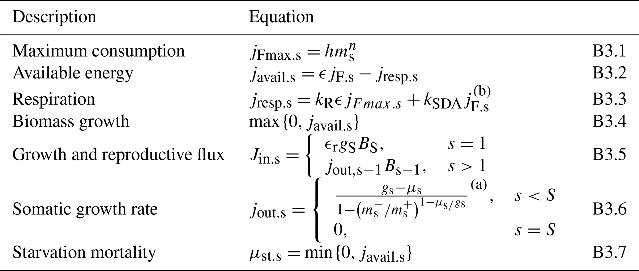
where multi = {all multicellular groups}. Here J_in (µg C L⁻¹ d⁻¹) is the mass flux into the size class, which equals the mass flux out of the previous class, except for the first class where it is the reproductive flux. The other fluxes are “pure” rates in units of 1 per day: j_out.i is the flux out of a size class, g_i is the biomass accumulation rate, and μ₀ is background mortality. The fluxes and the mortalities are calculated from the consumption by predation (Eq. 2) and the predation mortality (Eq. 3), and are detailed in Table B3.

3.4 Particulate organic matter (POM)

Particulate organic matter is produced by losses from plankton (Fig. 1). The POM has the same C:N ratio as the plankton, meaning that POM does not transport silicate. Instead, all silicate that should have gone to POM is considered lost to the deep sea and therefore also lost from the model. POM is generated from several sources (Fig. 4): (1) a fraction 1−γ₂ of cells dying from lysis; (2) multicellular plankton produce POM from sloppy feeding, fecal pellets (incomplete assimilation) and from the losses due to inefficient reproduction (egg mortality); (3) a fraction ${\mathit{\gamma }}_{\mathrm{POM}}=\mathrm{1}-{\mathit{\gamma }}_{\mathrm{HTL}}$ of the losses from higher trophic level mortality is assumed to be fecal pellets routed to POM. Particulate organic matter is lost from remineralization with a rate r_POM and from grazing by copepods:

$$\begin{array}{}\text{(14)}& \begin{array}{rl}{\displaystyle \frac{\mathrm{d}{B}_i}{\mathrm{d}t}}& =\sum _j\left[\left(\mathrm{1}-{\mathit{\gamma }}_{\mathrm{2}}\right){\mathit{\mu }}_{\mathrm{2}.j}+\left(\mathrm{1}-{\mathit{\gamma }}_{\mathrm{F}}\right)J_{\mathrm{Floss},j}\right.\\ & \left.+\left(\mathrm{1}-{\mathit{\gamma }}_{\mathrm{HTL}}\right){\mathit{\mu }}_{\mathrm{HTL},j}\right]B_i+\sum _{\mathrm{S}\in \mathrm{multi}\mathrm{adults}}\left(\mathrm{1}-{\mathit{ϵ}}_{\mathrm{R}}\right)g_{\mathrm{S}}\\ & B_{\mathrm{S}}-\left(r_{\mathrm{POM}}+{\mathit{\mu }}_{\mathrm{pr}.i}\right)B_i,i\in \mathrm{POM},\end{array}\end{array}$$

where index “S” indicates the last (adult) size class in each copepod population. Parameters are given in Table B5.

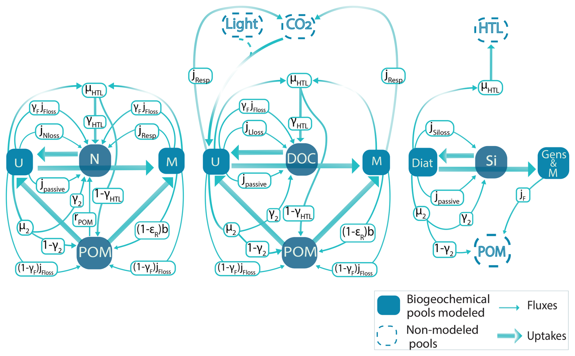
Figure 4 Representation of nitrogen, carbon and silica fluxes in unicellular (generalists and diatoms) (U) and multicellular (M) plankton. All rates are in units day⁻¹. In the chemostat setup POM sinks out to the deep (Eq. 20). The j's represent direct losses, the μ's represent mortalities, γ's represent fractioning of a flux into different pools (e.g. between direct remineralization and to POM), $b=J_{\mathrm{in}.1}/m_{\mathrm{egg}}$ is the copepod birth rate, and ε_F is feeding efficiency. j_Xloss refers to the losses of N and Si when growth is negative, and surplus carbon from photosynthesis to DOC. Note that POM does not contain silicate, instead all silicate fluxes that should have gone into POM are considered lost to the deep sea, therefore also absent in the model. Similarly, we assume that none of the silica in diatoms is assimilated by their predators and is instead directly remineralized.

3.5 Biogeochemical dynamics

The dissolved state variables are taken up through diffusive encounter and replenish with the losses from the plankton groups (Fig. 4). The equations for the dissolved phases of nitrogen, DOC, and silicate are:

$$\begin{array}{}\text{(15)}& {\displaystyle }\begin{array}{rl}{\displaystyle \frac{\mathrm{d}N}{\mathrm{d}t}}& =\left[\sum _{i\in \mathrm{uni}}\left(-j_{\mathrm{N},i}+j_{\mathrm{Nloss},i}+j_{\mathrm{passive},i}+{\mathit{\gamma }}_{\mathrm{F}}{j}_{\mathrm{Floss},i}\right.\right.\\ & \left.+{\mathit{\gamma }}_{\mathrm{2}}{\mathit{\mu }}_{\mathrm{2},i}\right)B_i+{\mathit{\gamma }}_{\mathrm{HTL}}{\mathit{\mu }}_{\mathrm{HTL}}\sum _{i\in \mathrm{multi}}{B}_i+r_{\mathrm{POM}}\\ & \left.\sum _{i\in \mathrm{POM}}{B}_i\right]{\displaystyle \frac{\mathrm{1}}{{\mathit{\rho }}_{\mathrm{C}:\mathrm{N}}}}\end{array}\text{(16)}& {\displaystyle }\begin{array}{rl}{\displaystyle \frac{\mathrm{d}C}{\mathrm{d}t}}& =\sum _{i\in \mathrm{uni}}\left(-j_{\mathrm{DOC},i}+j_{\mathrm{passive},i}+j_{\mathrm{Lloss},i}+{\mathit{\gamma }}_{\mathrm{F}}{j}_{\mathrm{Floss},i}\right.\\ & \left.+{\mathit{\gamma }}_{\mathrm{2}}{\mathit{\mu }}_{\mathrm{2},i}\right)B_i\end{array}\end{array}$$

$$\begin{array}{}\text{(17)}& \begin{array}{rl}{\displaystyle \frac{\mathrm{d}S}{\mathrm{d}t}}=& \left[\sum _{i\in \mathrm{diatoms}}\left(-j_{\mathrm{Si},i}+j_{\mathrm{Siloss}.\mathrm{i}.i}+j_{\mathrm{passive},i}+{\mathit{\gamma }}_{\mathrm{2}}{\mathit{\mu }}_{\mathrm{2},i}\right)B_i\right]\\ & {\displaystyle \frac{\mathrm{1}}{{\mathit{\rho }}_{\mathrm{C}:\mathrm{Si}}}}.\end{array}\end{array}$$

We have checked that all nutrients are conserved within an error close to numerical noise in Eqs. (12)–(17), while accounting for losses of silicate to the deep sea.

3.6 Temperature

Temperature T (°C) influences the physical and the metabolic processes of all groups in the model. The influence of temperature is described via Q₁₀ corrections to the parameters from a reference temperature of 10° as:

$$\begin{array}{}\text{(18)}& Q\left(T\right)=Q_{\mathrm{10}}^{\left(T-\mathrm{10}\mathit{°}\right)/\mathrm{10}\mathit{°}}.\end{array}$$

The only physical process influenced by temperature is the diffusion rate of dissolved matter (DOC, Si, and nitrogen) towards the cell, which has a Q₁₀=1.5 (Serra-Pompei et al., 2019). This means that the parameter α_N is corrected by temperature (Table B2). The other temperature correction is on metabolic rates by Q₁₀=2. The affected metabolic rates are: the basal metabolic rate (j_R for unicellulars and k_R for multicellulars), the maximum synthesis rates (α_max and h respectively), and the remineralization rate of POM r_POM. Applying temperature corrections on the individual processes means that the temperature response of division rate and growth are emergent and typically do not follow a Q₁₀ relation (Serra-Pompei et al., 2019; Andersen and Visser, 2023).

3.7 Embedding within ocean physics

The core NUM model library solves the state-variable equations (Eqs. 12–17) and can be embedded into a full circulation model. The library provides three simulation environments: chemostat (steady state and seasonal), water-column, and global. All environments, except the steady state chemostat, are implemented based on the transport matrix method (TMM) (Khatiwala et al., 2005; Khatiwala, 2007). The transport matrix method is a computationally cost-efficient offline numerical scheme to simulate ocean biogeochemical tracers, where a sparse matrix represents the advective-diffusive transport of a passive tracer. The transport matrix approach is a reliable alternative to conventional ocean general circulation models that reproduces reasonably well both the mean spatial and seasonal patterns of biogeochemical tracers in the ocean (Kvale et al., 2017). The NUM library employs the monthly resolved MITgcm transport matrices in a coarse resolution of 2.8°×2.8° and 15 vertical layers (Dutkiewicz et al., 2005), and a higher resolution of 1°×1° with 21 vertical layers (ECCO) (Forget et al., 2015). Both setups provide monthly transport matrices with a transport time step of 0.5 d. Sinking of POM is resolved with an implicit first-order upwind scheme (Press et al., 2007, Chap. 19). For the global and water-column simulations, the state-variable equations are solved with a forward Euler scheme with a simple predictor-corrector step to avoid negative values of the dissolved tracers, and a time step of 0.1 d. The bottom boundary conditions are closed for all living biological state variables and for DOC. POM is allowed to sink into the bottom. Nutrients (nitrogen and silicate) are nudged towards a fixed concentration at the bottom:

$$\begin{array}{}\text{(19)}& u_{t+\mathrm{1}}=u_t+\mathit{\kappa }{\displaystyle \frac{\mathrm{\Delta }t}{\mathrm{\Delta }z}}\left(u_{\mathrm{bottom}}-u_t\right),\end{array}$$

where u is the state variable (N or S), t is the time step, Δt is the transport time step (0.5 d), Δz is the thickness of the bottom layer, $\mathit{\kappa }=\mathrm{1}/\mathrm{365}$ m d⁻¹ is the relaxation rate, and u_bottom is the bottom concentration taken from World Ocean Atlas climatologies (Reagan et al., 2023).

The chemostat environment models the upper mixed layer which mixes with an unresolved deep layer, with a mixing rate d (d⁻¹) (Evans and Parslow, 1985). The deep layer concentrations of nutrients are fixed, N_deep and S_deep, and the concentration of DOC is zero. Unicellular organisms are mixed out of the upper layer, while the multicellular organisms are assumed to stay in the upper layer. POM is mixed out of the surface layer but also sinks out with a rate $v/M$, where v (m d⁻¹) is the sinking velocity and M (m) the thickness of the mixed layer. The governing equations are solved with the internal matlab Rosenbrock 2nd order stiff solver:

$$\begin{array}{}\text{(20)}& {\displaystyle \frac{\mathrm{d}{B}_i}{\mathrm{d}t}}=f_i(L,T,\mathbf{B})+\underset{\mathrm{for}\mathrm{nutrients}\mathrm{and}\mathrm{uni}.}{\underbrace{d\left(B_{\mathrm{deep}.i}-B_i\right)}}-\underset{\mathrm{for}\mathrm{POM}}{\underbrace{{\displaystyle \frac{v}{M}}{B}_i}},\end{array}$$

where the first term $f_i(L,T,\mathbf{B})$ is the right-hand-side of the state-variable equations (Eqs. 12–14), which depends on light L, temperature T and the set of all the state variables B. Finally, the chemostat can be run in a seasonal environment where light, temperature, and mixing rate d vary with time and are extracted from the transport matrix. In high latitude environments it is necessary to disable the mixing of unicellular plankton to the deep layer to allow them to survive the winter period.

3.8 Model setup and numerical solution

The model framework allows for a flexible combination of the four groups. A model setup requires at least one unicellular group (generalists or diatoms), and may include POM and a number of copepod groups. The default NUM model setup used here involves all four groups. Each group contains a number of size classes and the model results depend, to some degree, on the number of size classes used in the unicellular groups (Fig. 5a and b) and in the copepod groups (Fig. 5c and d). Further, it depends on the number of active-copepod and passive-copepod groups (Fig. 5e and f). The number of size classes and copepod groups in the default NUM model setup is chosen such that the overall results, in terms of size spectra (Fig. 5a, c and d) and ecosystem function (Fig. 5b, d and f), do not change considerably upon the addition of more classes or groups. The setup includes 10 size classes of generalists, 10 size classes of diatoms, two passive copepod groups (adult sizes 0.2 and 5 µg C; prosome lengths 320 and 1040 µm), and three active copepod groups (1, 32, and 1000 µg C; prosome lengths from 584 and 7200 µm), where each group is discretized in 6 size-classes representing the growth in body mass. The number of state variables adds up to a total of 54.

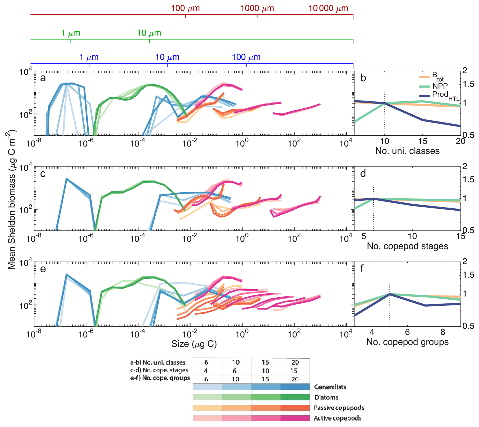
Figure 5 Sensitivity of the model to number of unicellular size classes (a, b), number of copepod stages (c, d), and number of copepod groups (e, f). The left column of panels (a, c, e) show the Sheldon size distributions (biomass normalized by the width of each size bin; Andersen and Visser (2023, Box V)) and the right column (b, d, f) shows total biomass (orange), NPP (green), and HTL production (dark blue) normalized by the value in the standard setup (vertical dashed line). All runs are from a simulation of the water column model at 60° N and 40° W. Color intensity indicates number of classes/groups. In the left panels, blue shades represent generalists, green diatoms, orange-red passive copepods and magenta active copepods. The colored axes on top show the lengths of the three groups: equivalent spherical diameter for generalists (blue) and diatoms (green), and prosome length for copepods (red).

Running the NUM model from the matlab interface proceeds in four steps: (1) setting up the simulation type (i.e., choosing which size spectra groups to simulate), (2) setting up the simulation environment (chemostat, water column, or global), (3) running the model, and (4) plotting the output:

p = setupNUMmodel(bParallel=true);
% Model setup
p = parametersGlobal(p);
% Model environment
sim = simulateGlobal(p);
% Run simulation
plotSimulation(sim);

All parameters are encapsulated in the |p| structure, which is passed to the simulation (in this example a global simulation). The simulation returns the entire output in the |sim| structure which is passed on to other functions for analysis or plotting. These two structures are documented on the github site and all functions are documented in their |help| pages.

3.9 Calibration and evaluation data

All parameters of the plankton groups are based on first principles or cross-species comparisons (Andersen and Visser, 2023; Serra-Pompei et al., 2020). While these parameters are uncertain (explored by Hansen et al. (2025)), they are not expected to vary spatially. However, some of the extrinsic parameters either have no first-principle arguments or data, and/or are varying spatially. These extrinsic parameters together mold the overall function of the community: the global average light extinction coefficient by water k_w without feedback from plankton, the average POM sinking velocity v, and the higher trophic level mortality μ_HTL.0. These variables conjointly determine the total biomass and production of the global model: lower light extinction increases gross primary production, lower sinking velocity decreases the remineralisation depth and thereby increases the amount of primary production. Decreasing the mortality by higher trophic levels increases the copepod biomass, which influences the unicellular spectrum through a trophic cascade (Fig. E5). In nature, the values of these three variables vary on a global scale, but here they are kept constant. Consequently, we must calibrate to find reasonable global average values. The calibration algorithm minimizes the error between modeled and observed values, based on the following steps:

First we compute the mean error between in situ data Q_obs to modeled output Q_model for three metrics: picoplankton (i=1), POC (i=2), copepod biomass (i=3) in varying space and time for each metric, such that the number of available measurements of each metric i is n_i, and each distinct measurement is j. This calculation is represented in the first addend in Eq. (21). The datasets are described below. The datasets used in this part of the algorithm are: (1) picophytoplankton biomass (organisms with a diameter less than 2 µm) between 0 and 10 m depth from water samples between 1997 and 2014, across all latitudes mainly in the Atlantic Ocean (Fig. D3) (Martínez-Vicente et al., 2017b); (2) Particulate Organic Carbon (POC) biomass of all plankton and detritus particles with a radius between 0.35–15 µm from the GO-POPCORNv2 dataset (Tanioka et al., 2022) from cruises (2011–2020) across all major ocean basins, spanning from 70° S to 55° N (Fig. D2); (3) copepod biomasses across the Atlantic Meridional Transect cruises (López and Anadón, 2008).

$$\begin{array}{}\text{(21)}& \begin{array}{rl}\mathit{\epsilon }=& {\displaystyle \frac{\mathrm{1}}{\mathrm{6}}}\left[\sum _{i=\mathrm{1}}^{\mathrm{3}}{\displaystyle \frac{\mathrm{1}}{n_i}}\sum _j^{n_i}\log \left({\displaystyle \frac{Q_{\mathrm{model}.ij}}{Q_{\mathrm{obs}.ij}}}\right)+\sum _{k=\mathrm{1}}^{\mathrm{3}}\log \right.\\ & \left.\left({\displaystyle \frac{P_{\mathrm{NPPmodel}.k}}{P_{\mathrm{NPPobs}.k}}}\right)\right].\end{array}\end{array}$$

Second, we select three distinct locations in the ocean that correspond to an oligotrophic, a eutrophic and a seasonally varying environment to compare the mean error between the annual averages of satellite derived NPP and modelled NPP (P_NPPmodel): an oligotrophic location (22° N, 158° E), a eutrophic location (5° S, 5° E), and a seasonal location (60° N, 40° W). At these sites, the annual averaged NPP over the entire water column from CAFE is approximately 200, 1000, and 500 mg C yr⁻¹, respectively. This comparison with NPP appears in the second addend of Eq. (21). P_NPPobs corresponds to annual averages (2002–2021) from satellite observations processed with the CAFE model, selected due to its better performance on a global average relative to other satellite-derived NPP models (Silsbe et al., 2016).

The net primary production is calculated in the model as the amount of carbon that is fixed by photosynthesis minus what is used for respiration:

$$\begin{array}{}\text{(22)}& P_{\mathrm{NPP}}=\sum _{i\in \mathrm{uni}}\max \left\{\mathrm{0},\left(j_{\mathrm{L}.i}-j_{\mathrm{resp}.i}\right)B_i\right\}.\end{array}$$

This definition appears simple but there are two important comments. First, all mixotrophic metabolic costs are included in the respiration (j_resp) that is subtracted from the fixed carbon (j_L), including the costs of feeding and DOC uptake. This is different from the usual thinking about primary production, which implicitly assumes that primary production only occurs by obligate phototrophs. Second, it should be noted that the definition does not include all primary production. Some carbon is lost to DOC during the uptake process (Fig. 4b), which can fuel osmotrophic biomass production. The DOC part of primary production can contribute a substantial portion of measured primary production (Karl et al., 1998). Adding this potential carbon production into the definition can be achieved by replacing j_L with $j_{\mathrm{L}}{\mathit{ϵ}}_{\mathrm{L}}^{-\mathrm{1}}$. However, we refrain from including DOC NPP, which may result in underestimating by the model compared to measured NPP at oligotrophic sites.

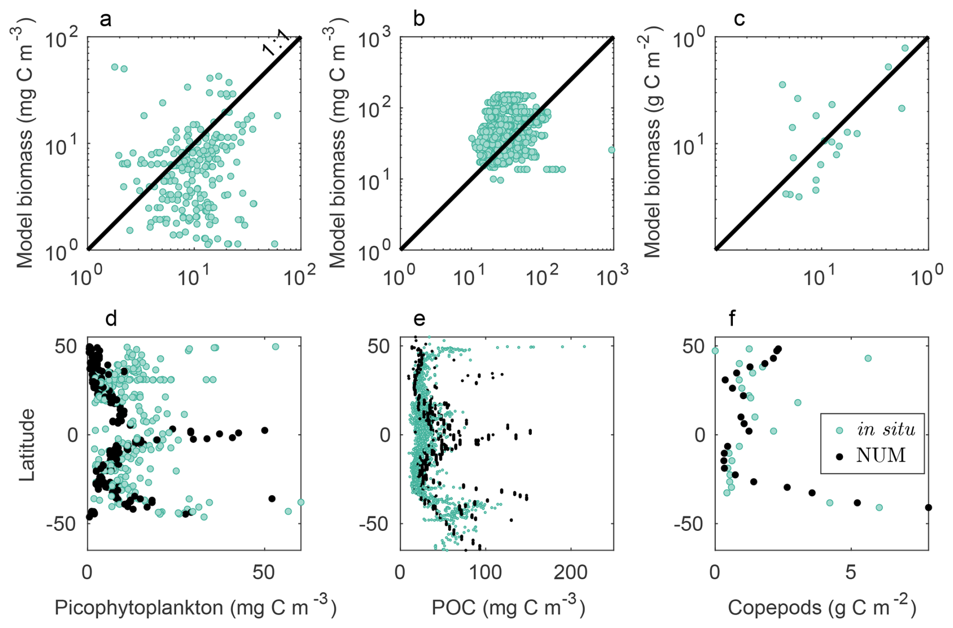
Figure 6 Comparison of model biomass output to in situ calibration data for biomasses of picophytoplankton (a, d), particulate organic carbon (b, e), and copepods (c, f). The top row shows modeled biomasses on the y axis and observations on the x axis. The bottom panels show the latitudinal variation of biomasses. Mean biases are −0.70 (a), 0.38 (b), and 0.016 (c), calculated from Eq. (21).

After the initial calibration of the three parameters we evaluate the performance of the NUM model using a second set of observations. For the performance evaluation we use observations of nano- and microplankton from three Atlantic Meridional Transects cruises (Rodríguez-Ramos et al., 2015), a meta-analysis of global mesozooplankton biomass distribution (Moriarty et al., 2013), and annual averages of surface nutrients from the World Ocean Atlas (Reagan et al., 2023). To validate the global diatom distributions we use the Copernicus Global Ocean Colour satellite product (CMEMS, 2025). This product provides the surface chlorophyll divided between groups. We use the ratio between the total chlorophyll and the diatom chlorophyll as a proxy for the ratio between modeled phytoplankton and diatom biomasses. This use assumes that the biomass:chlorophyll ratio is roughly similar between diatoms and other phytoplankton at the same site, but allows for variation in the ratio between sites. However, the satellite observations only capture the first few meters of the surface, whereas the top layer in the global model is a mean over the top 50 m. This evaluation data-set will therefore be inaccurate in the areas with a deep chlorophyll maximum.

4 Results

Simulations are initiated with concentrations of inorganic nitrogen and silicate from the World Ocean Atlas (Reagan et al., 2023). Biomass distributions equilibrate quickly and are well converged after 10 years (Fig. E6b and d). Deep nutrient concentrations are on a long slow transient, particularly away from seasonal environments (Fig. E6a and c). The value of the bottom boundary condition exhibits a very weak effect on the biomass and net primary production (Fig. E7). The simulations presented in the following are after 10 years of simulation with the standard NUM model setup (Sect. 3.8).

We first show the model calibration followed by the model global biomass distributions. We then assess performance with evaluation data, show how the three model environments (global, water column, and chemostat) compare, and finally show outputs related to the physiological dynamics of the organisms in the model.

4.1 Model calibration

The calibration gave an optimal light extinction coefficient of 0.06 m⁻¹, a sinking velocity of 19 m d⁻¹, and a coefficient of higher trophic level mortality of 0.017 L(µg C d)⁻¹. The response of the model to changes in each calibration parameter is shown in Fig. E5. The calibrated model produces biomasses of picoplankton, POC, and copepods which are in the correct order of magnitude of the observations (Fig. 6a–c). Though the three parameters are calibrated to be constant in time and space, the model does produce latitudinal patterns in accordance with the observed patterns (Fig. 6d–f: elevated biomass at temperate latitudes (−50 and 50°) and around Equatorial upwelling. The modeled copepod biomass approximates observations at temperate latitudes, however, it underestimates copepod biomass in the Equator.

4.2 Modeled biomass and productivity

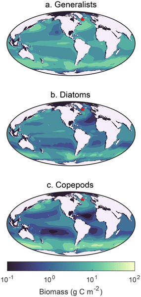
The model captures general global-scale biomass patterns, with higher concentrations of unicellular and multicellular plankton in high-latitude seasonal environments and equatorial upwelling areas and the lowest biomasses in oligotrophic gyres (Fig. 7). These patterns are mirrored in satellite-derived NPP estimates (Fig. 8). Satellite production of NPP is subject to a systematic bias (Dierssen, 2010), and further the panels b–e highlight the big variation between satellite observation products. Nevertheless, one unrealistic pattern in the model that clearly stands out is the very high biomass and production in the Southern Ocean.

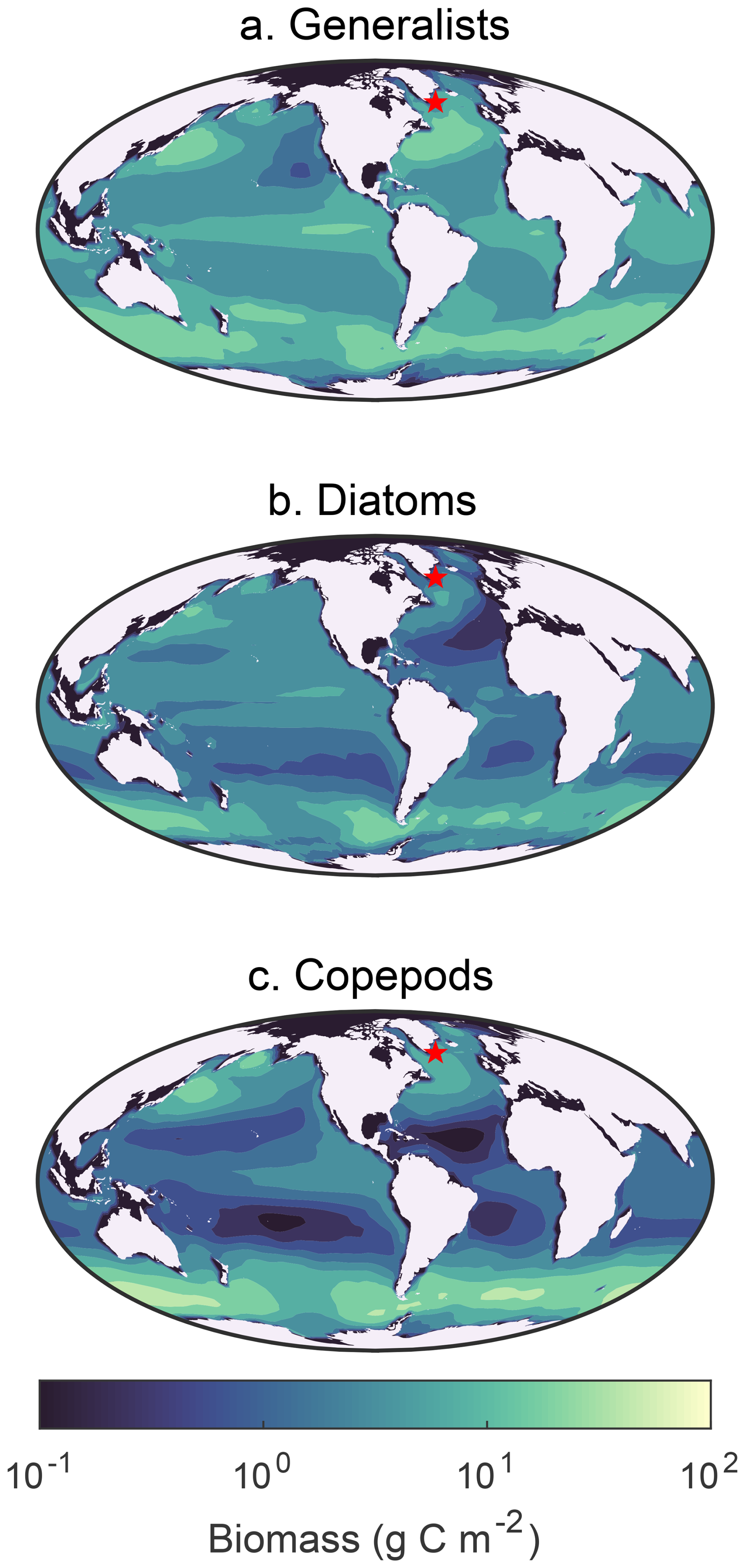
Figure 7 Global annual average biomass of (a) generalists, (b) diatoms and (c) copepods. The red star indicates the location (60° N, 40° W) that is used for evaluate the seasonal dynamics in later figures.

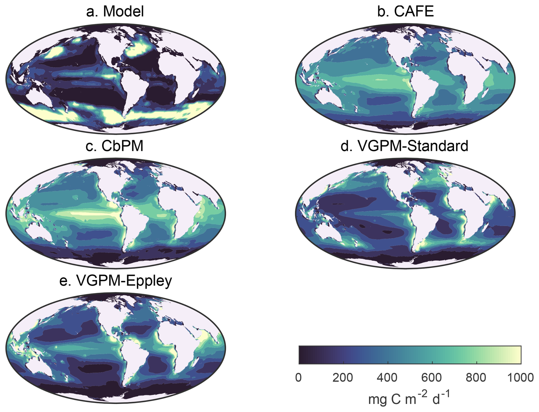
Figure 8 (a) NUM annual mean NPP, (b) CAFE estimated annual mean NPP (Silsbe et al., 2016), (c) CbPM estimated annual mean NPP (Westberry et al., 2008), (d) VGPM-Standard estimated annual mean NPP (Behrenfeld and Falkowski, 1997), and (e) VGPM-Eppley estimated annual mean NPP (Behrenfeld and Falkowski, 1997), all datasets from (, ). Units are mg C m⁻² d⁻¹.

4.3 Model evaluation

Turning to the evaluation data from the Atlantic transects, we see that the model captures the right order of magnitude of nano- and micro-plankton biomasses summed together (Fig. 9). In these data, increased biomass around equatorial upwelling is less than expected, which is also reproduced by the model. However, the model overestimates plankton biomass at higher latitudes compared to the AMT 14 cruise (Fig. 9d), where samples were collected during May. At the global scale, the simulated average macrozooplankton concentration (copepods, larvae, and krill with a prosome length > 2 mm) is of the correct order of magnitude compared to observations, although the correlation is weak (Fig. 10).

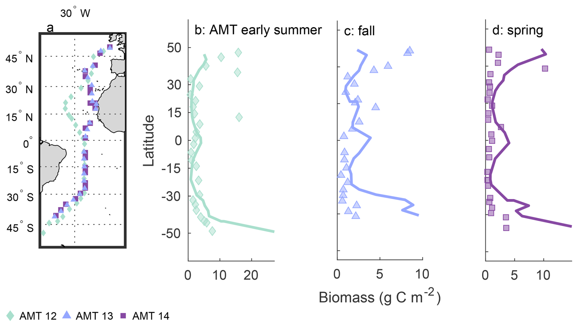
Figure 9 Biomass of nano- (2–20 µm radius) and micro-plankton (20–200 µm radius) of the model (line) compared to AMT data (markers). (a) Transects of the different AMT cruises, (b) AMT 12: May–June, (c) AMT 13: September–October, (d) AMT 14: May. The modeled biomass is the depth-integrated average of the respective months for each cruise, extracted from the final year of a 10-year global simulation.

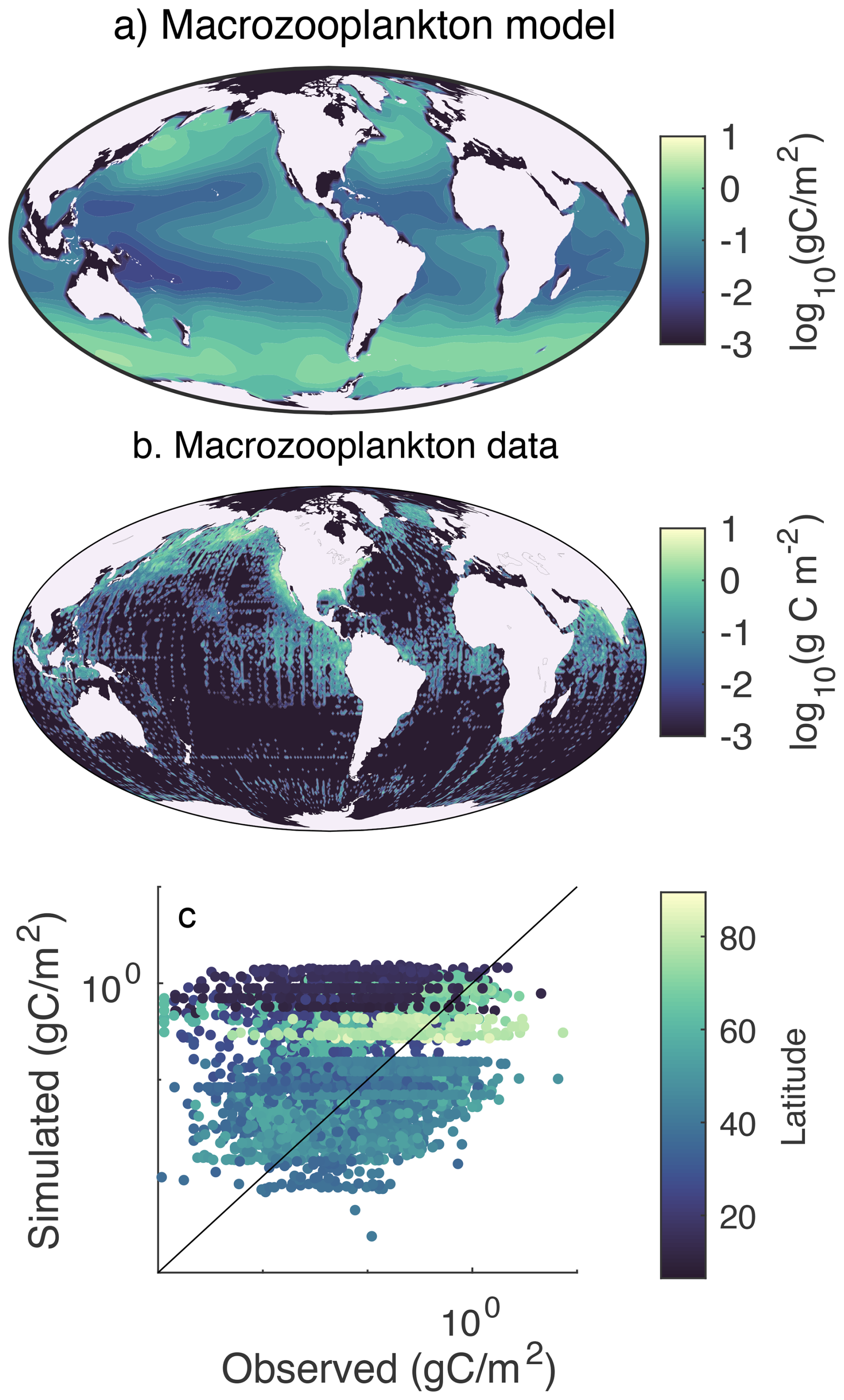
Figure 10 Annual mean macrozooplankton biomass, (a) model output (integrated over the top 170 m) and (b) observation data from Moriarty et al. (2013) (integrated over the top 170 m), compared at different latitudes in panel (c).

The model resolves nitrogen in a simplified manner without accounting for its different forms (i.e. nitrate, nitrite, ammonia). We have chosen nitrate for the comparisons because it is considered to be the main nitrogenous compound utilized for primary production (Lenton and Watson, 2000). The model captures the spatial patterns in annual mean nitrogen and silicate concentrations at the surface (Fig. 11) with high values in the North Atlantic and Southern Ocean and lower at the oligotrophic gyres. In addition, it reproduces elevated concentration in equatorial upwelling areas. However, the modeled values are generally much lower than the observed values. This is likely due to very efficient uptakes of nutrients by unicellular plankton in the model, which leads to low limiting nutrient concentrations (low “R^*” sensu, Tilman, 1980). This effect was also observed in the analysis of the generalist level (Andersen and Visser, 2023).

Figure 11 Annual mean concentrations of (a, b) nitrate and (c, d) silicate in the top 5 m. World Ocean Atlas (WOA) (Reagan et al., 2023) observations (a, c) compared to model output (b, d).

The model captures the high surface diatom : phytoplankton ratio in high latitudes but overestimates diatoms in mid latitudes (Fig. 12). This concurs with observations in the Pacific (Endo et al., 2018) and the Atlantic Oceans (Marañón et al., 2000). The overestimation in mid latitudes could be an artifact of the satellite measurements only seeing the very surface waters, whereas the top layer in the simulations performed here is the upper 50 m. Further, data from the Continuous Plankton Recorder (CPR) survey (Reid et al., 2003) shows that diatoms constitute a fraction up to about 50 % of the total phytoplankton biomass throughout the North Atlantic (Barton et al., 2013), in correspondence with the model simulations.

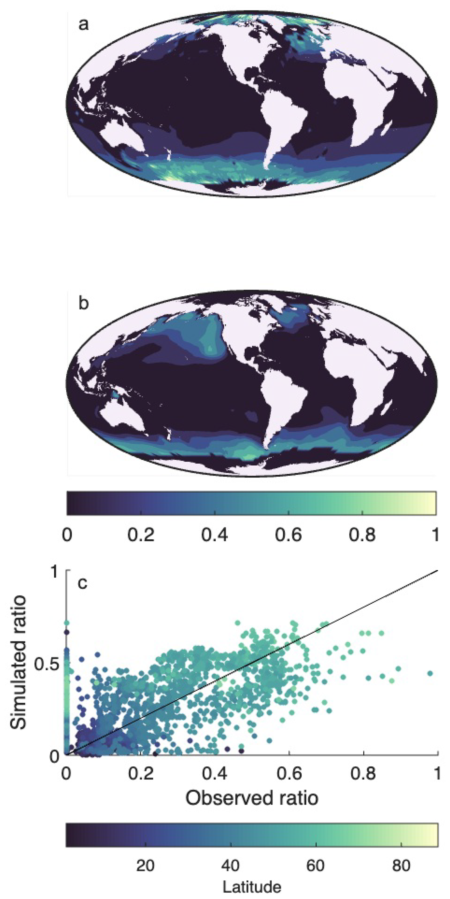
Figure 12 Observed (a) and simulated (b) global surface distribution of the diatom:phytoplankton biomass ratio (Eq. 24). Panel (c) compares the observations and simulations with the color indicating latitude. The observation is a climatological mean from 1998 to 2024 of surface chlorophyll (see text for a description of the observation data set.).

4.4 Model simulations

The unicellular NUM model's output differs from traditional biogeochemical plankton models: instead of having state variables of bacteria, phytoplankton, and zooplankton, the NUM model resolves generalists and diatoms. While the diatoms are obligate phytoplankton (including DOC uptake), the trophic strategies of the generalists are dynamic and an emerging property of the model. However, common terminology and most models explicitly resolve state variables of bacteria, phytoplankton, and zooplankton. To relate the model's output to the aforementioned groups, we can estimate bacteria, phytoplankton, and zooplankton biomass from the generalists and diatoms, by weighing each size class with the fraction of carbon assimilation from DOC (bacteria-like), photosynthesis (phytoplankton-like), and phagotrophy (zooplankton-like):

$$\begin{array}{}\text{(23)}& {\displaystyle }& {\displaystyle }{B}_{\mathrm{bact}}=\sum _i{\displaystyle \frac{j_{\mathrm{DOC}}}{j_{\mathrm{C}}}}{B}_i\text{(24)}& {\displaystyle }& {\displaystyle }{B}_{\mathrm{phyto}}=\sum _i{\displaystyle \frac{j_{\mathrm{L}}}{j_{\mathrm{C}}}}{B}_i\text{(25)}& {\displaystyle }& {\displaystyle }{B}_{\mathrm{zoo}}=\sum _i{\displaystyle \frac{j_{\mathrm{F}}}{j_{\mathrm{C}}}}{B}_i,\end{array}$$

where $j_{\mathrm{C}}=j_{\mathrm{DOC}}+j_{\mathrm{L}}+j_{\mathrm{F}}$ (Fig. 13a–c).

Figure 13 Annual depth-integrated mean biomass in the model: (a) bacteria biomass, (b) phytoplankton, (c) zooplankton, including unicellular plankton (mixotrophs and phagotrophs) and copepods, all calculated from Eqs. (23)–(25).

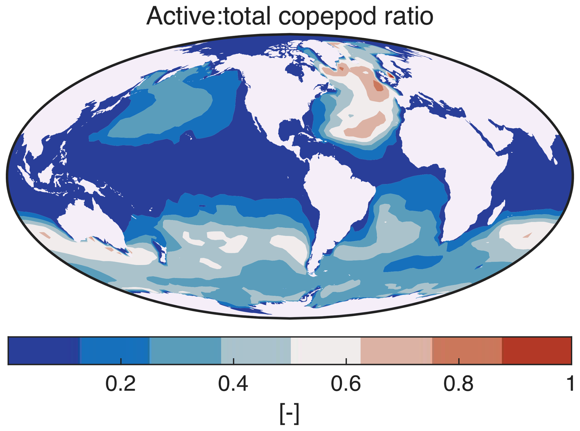
Figure 14 Ratio of active-feeding copepods to total copepod biomass.

The copepod community is dominated by active copepods in higher latitudes (Fig. 14) and by passive (ambushing) copepods in oligotrophic gyres. In equatorial regions the presence of active copepods varies in different oceans. In the Equatorial Atlantic active copepods occupy between 50 % and 60 % of the multicellular plankton community. Lastly, active copepods occupy 60 % to 80 % of copepods along boundary currents in the Pacific, namely the California Current east and Kuroshio Current west.

4.5 Comparison of environment setups

We compared runs of the water-column and seasonal chemostat model setups to the output from a global simulation at a high latitude location (Fig. 15) that is seasonally stratified. We chose a seasonally stratified location because it exhibits the succession of oligotrophic and eutrophic conditions throughout the year. The seasonal dynamics of total biomass show similar dynamics in the global and water-column simulations (Fig. 15a and c): a bloom in spring throughout the water column, followed by a deeper production maximum in summer, and terminated by a smaller autumn bloom. The spring bloom of diatoms is terminated first by silicate limitation, and the generalist bloom is terminated a bit later by nitrogen limitation (Fig. E4a and b). Contributing to the demise of the bloom is the grazing by copepods, which become established over summer (Fig. E4f–h). The deep maximum is less well represented in the global simulation, with only 13 vertical levels, than the water column simulation with 21 levels.

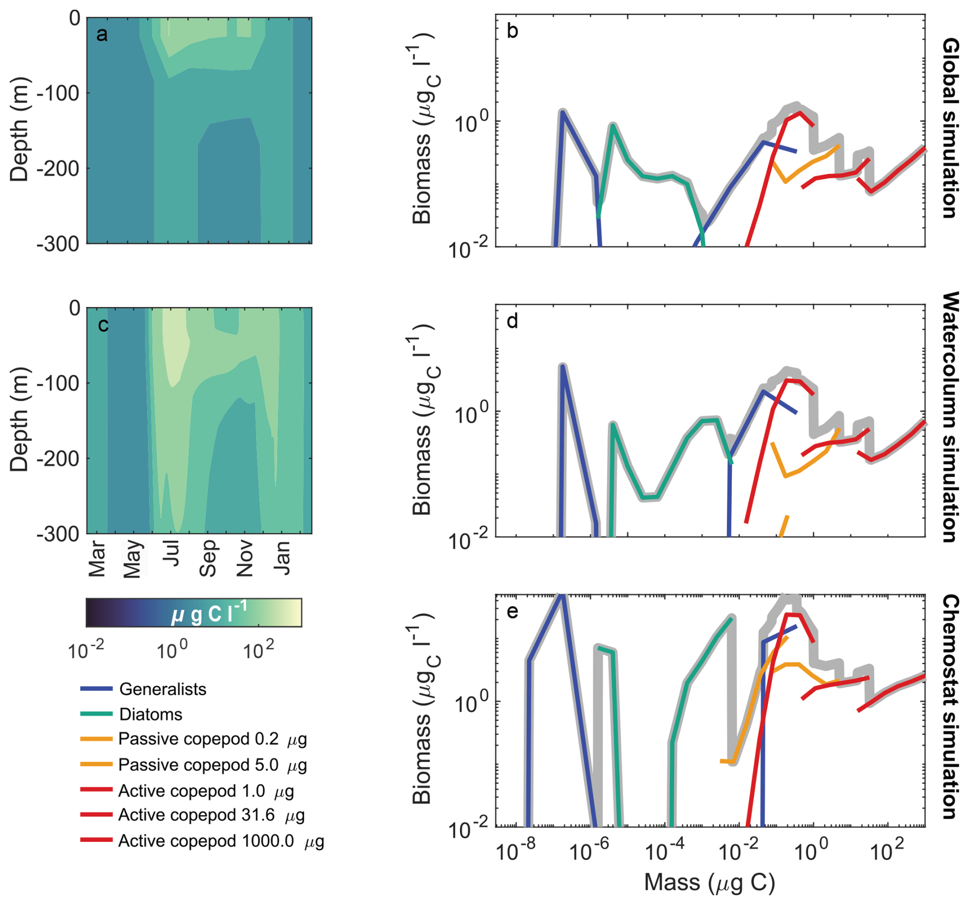
Figure 15 Model output for a 10-year simulation in the global, water column, and chemostat environments at a seasonally stratified location (60° N, 40° W) (red star in Fig. 7). (a) Total biomass in a water column extracted from the global simulation. (c) Total biomass in the same water column, but extracted from the water-column simulation. (b, d, e) Sheldon spectrum of the community from global, water-column, and chemostat simulations at 5 m depth and geometrically averaged over the last year. See Fig. 5 for an indicative length axis.

The size spectra show an overall similar community structure in the global ocean, water column and chemostat simulations (Fig. 15b, d and e). The plankton biomass is generally higher in the chemostat simulations than in the global and water-column simulations. The physical mixing in the global and water-column models constitutes a loss term by exporting planktonic organisms to the deep water, where they die unless they are mixed back into the photic zone. In the seasonal chemostat this mixing does not occur. That healthy growing diatoms tend to have near-neutral buoyancy is well established (Gross and Zeuthen, 1948; Smayda, 1970). How they do it is also well established (Boyd and Gradmann, 2002). It is only when cells become stressed (e.g., low nutrients) and die that they start to succumb to gravity (Waite et al., 1992). The modelling assumption that diatoms while growing are neutrally buoyant is relatively robust. The difference in the modelling of mixing losses between chemostat simulations and the two other environments should be kept in mind when using the environments. Nevertheless, the output of the water column illustrates the same dynamics as the global at the same site, indicating that the water column model – which is naturally much faster than a global simulation – performs well. It should be noted, though, that the water column simulations perform best in seasonal environments. In less seasonal environments, the absence of lateral advection appears to result in too low production (Figs. E1 and E2).

4.6 Individual-level processes

The NUM library makes it possible to extract descriptions of the rates that drive the dynamics of each size class. Figure 16 shows the rates of the generalists, diatoms, and copepods from the chemostat simulation in Fig. 15d, with uptakes of resources (or prey) illustrated as positive rates and losses including mortalities as negative rates. Overall, the rates of uptakes and losses are much higher in the spring bloom (left column) than in the summer (right column). The spring panels portray strong predation pressure on the unicellular community (dashed red lines in Fig. 16a and b), indicating that the bloom is decaying at this time. The high predation is also reflected in high feeding rates of the copepod community (red lines in Fig. 16c and d). Therefore, the spring copepod community is acquiring biomass at the expense of the unicellular community. In contrast, during summer, the division and loss rates in the unicellular community are roughly equal (grey lines in Fig. 16e and f). This indicates a community in balance with little changes in biomass. Further, in the unicellular community, the figure shows how the trophic strategies change with cell size (Andersen et al., 2016): for the smallest cells, the acquisition of carbon is governed by DOC uptake (magenta lines), and dissolved nutrients (blue lines), in particular in the spring bloom (Fig. 16a and b). Larger sizes of generalists combine phototrophy (yellow lines) for carbon uptake for respiration with predation (red lines) for nitrogen and carbon for biosynthesis (and possibly respiration). Larger sizes of diatoms are purely phototrophic (negligible uptake of DOC) and are limited by nitrogen and silicate uptakes during summer.

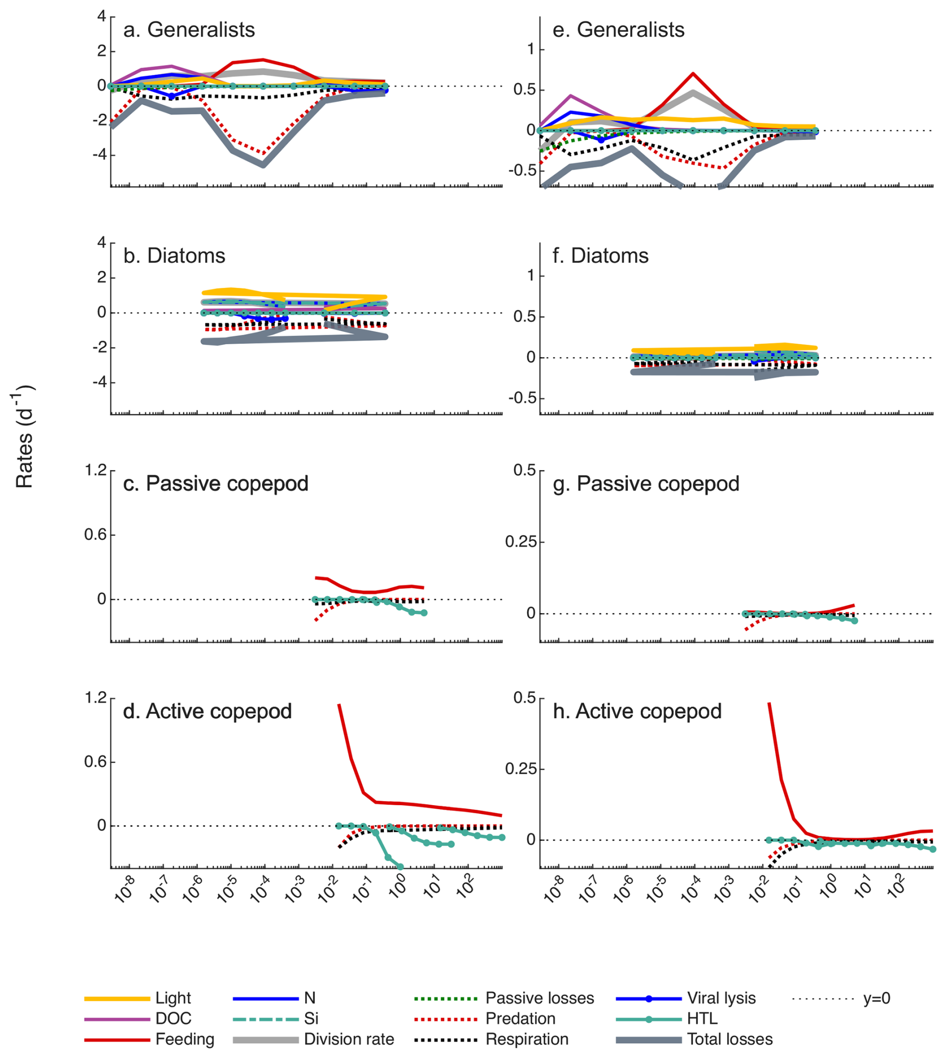
Figure 16 Gains and losses as a function of cell/body size in the spring bloom (April, a–d) and the summer (July, e–h) from the chemostat simulation in Fig. 15e. The lines above the horizontal dashed line shows gains either of carbon (from DOC uptake or photoharvesting; magenta and yellow), nutrients, silicate (blue and green), or a combination of carbon and nutrients from predation (red). The lines below the dashed lines shows losses of carbon from respiration (dashed black) or mortalities from predation (dashed red) or viral lysis (blue). The division rate is shown with thick grey. Note the differences in the y axes ranges between the left and right columns.

Figure 17 Metabolic budgets for generalists (left panels) and diatoms (right panels) in April (top panels) and July (bottom panels) extracted from Fig. 16 (and from the chemostat simulation in Fig. 15e). The division rate represents the uptakes that are used for synthesis of new biomass.

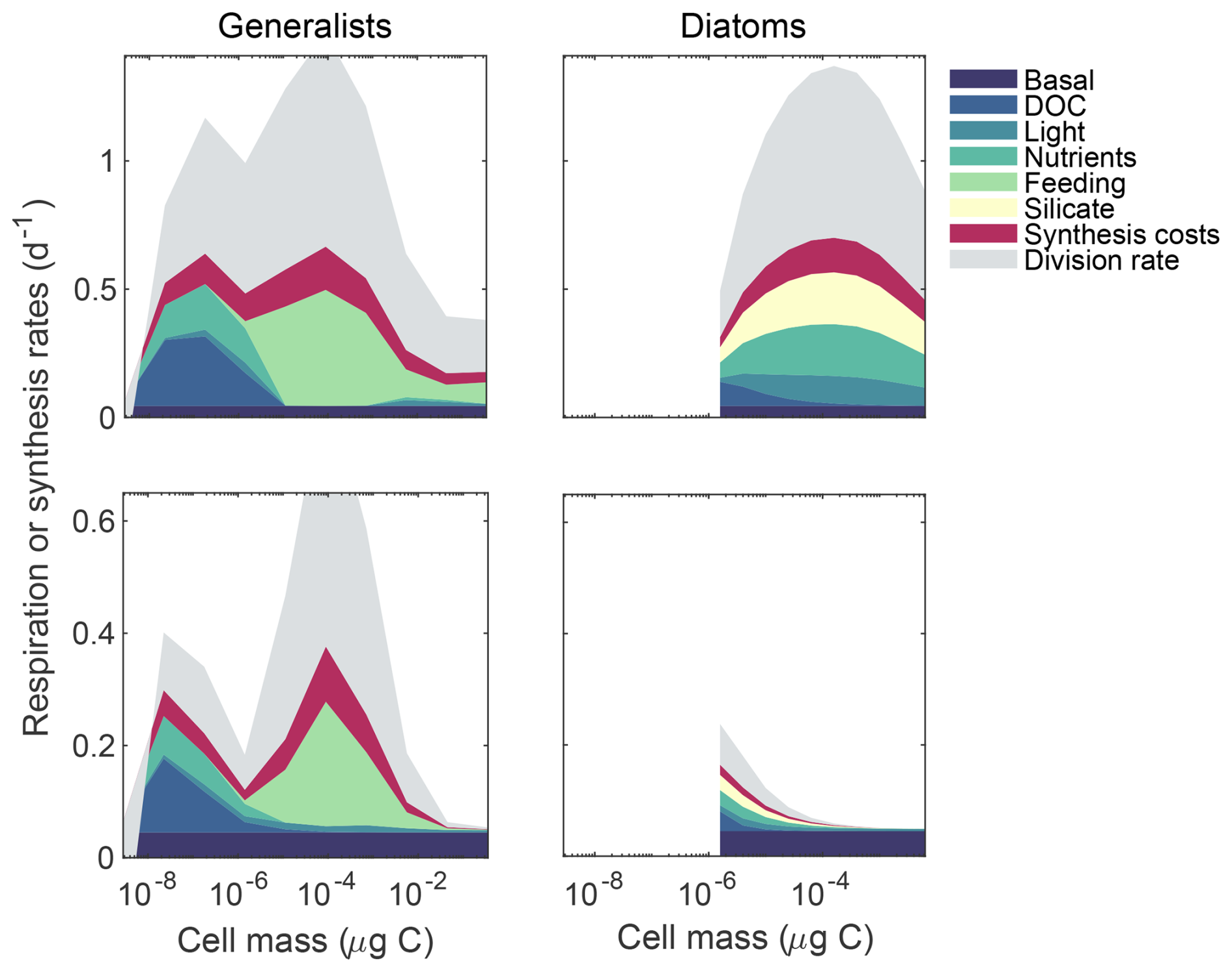
The regulation of uptakes by unicellular plankton (Sect. 3.2.2) entails that the respiration budget is resolved explicitly among the carbon used for synthesizing new biomass and different respiratory costs of basal metabolism, uptakes of dissolved nutrients and carbon, specific dynamic action of feeding (digestion), and costs of synthesizing new biomass (Fig. 17). In general, the synthesis of new biomass (the division rate) is one third of the total metabolic budget (Fenchel, 2013), while the respiratory costs are distributed among the different uptake costs, and a small portion is allocated to basal metabolism.

5 Discussion

We have presented a computational library for ecological modelling of plankton communities that resolves their utilization of resources, their trophic strategies, their size-structured population dynamics, and their production of dissolved and particulate organic carbon. The library includes a high-level interface to simulate the communities on global scale, in a water column, or in a chemostat. Because the model includes copepods, which are often weakly represented in biogeochemical models, the model lends itself to linking with fish production models, or to modelling the carbon pump arising from copepod fecal pellets and plankton carcasses. Overall the NUM model is an intermediate-complexity model laboratory for ecological simulations that is accessible to marine ecologists without biogeochemical or physical oceanography background. The focus here has been on the presentation of the general and flexible programming library and the calibration of the core NUM model setup.

The library has been designed with flexibility in mind. It can be run fully from a high-level programming language (mainly matlab). As the core library is written in Fortran, it is straight-forward to implement the model in a full circulation model (Hansen et al., 2025), for example using the FABM interface (Bruggeman and Bolding, 2014). Further, new size-spectrum groups can be added to the library. While POM described here is a single-state variable, the model does include a module to handle POM as an entire size spectrum. A more complex POM module is currently under development (Visser et al., 2024). Future extensions would be the inclusion of an iron nutrient tracer to limit the production in the Southern Ocean, a diazotroph spectrum to include nitrogen fixation, and a description of calcifiers.

Another flexible aspect of the NUM library is the possibility of performing simulations in three environmental settings: global, water column, and chemostat. Water-column or chemostat simulations are useful for making fast model development or trial simulations before moving to full global simulations. However, it should be noted that even though the three settings are based on the same transport matrix there are differences in the output between them. First, the seasonal variation of total biomass both in the global and water column simulations at a high-latitude location concur: a spring bloom throughout the water column, followed by a deeper plankton biomass maximum in summer (Yasunaka et al., 2022), and a moderate short autumn bloom. However, the global simulations reproduction of the deep maximum is coarser than in the water column, most probably due to a lower vertical resolution. While the structure of the water-column simulations corresponds relatively well with the global simulations in a strongly seasonal environment, they do not match well outside of high-latitude environments, probably due to the absence of advective processes in the water-column simulation. Further, we observe disparity in the size spectra of the community extracted from global, water column, and chemostat models. In particular, the dominance of large diatoms in chemostat simulations, emerges from the absence of mixing losses of plankton in the chemostat simulations, while mixing losses are present in water-column simulations. This finding points to the importance of a better understanding of plankton's ability to maintain a position in the photic zone despite vertical mixing.

Diatoms have been included here as a new size spectrum group. The module is based on an extension of the generalist module with the addition of a vacuole and a silicate shell. In this manner, the diatom module does not use any diatom-specific parameters, apart from the cost of silicate uptake, the size of the vacuole, the minimum and maximum size, and the vulnerability to predation, but shares all other parameters with the generalists. Further, silicate is not incorporated into the POM, it is therefore lost from the model. In light of this very simple description of diatoms, and the important omission of sinking silicate POM, the module performs quite well, as it captures the emergence of large diatoms during spring blooms in seasonal environments and their dominance in high latitudes (Figs. 7b and 14a). Nevertheless, while larger phototrophic diatoms appear in high latitude seasonal regions, they are missing in upwelling regions in the global and water-column simulations (though they do appear in chemostat simulations). The absence of phototrophic diatoms in upwelling regions simulated in the model is implausible, given their known prevalence in such nutrient-rich waters (Benoiston et al., 2017). We conjecture that the absence of large diatoms is due to mixing losses; in nature diatoms are able maintain their position in the water-column by active buoyancy regulation. However, in the global and water-column simulations, diatoms are mixed out. In contrast, the chemostat simulation ignores mixing losses of unicellular plankton. A future fix could be to include buoyancy control in the diatom module to avoid mixing diatoms out and thereby limiting their mortality. Finally, silicate should be included into the POM group. This would require another state variable to account for the variable stoichiometric composition of POM.

Our ambition has been to parameterize all processes within the unicellular and multicellular groups from considerations based on first principles or, if those are not available, from cross-species analysis of laboratory observations. This ambition is only partially realized. For the unicellular groups, the parameters and processes related to uptakes are well characterized by first principles of diffusion, light encounter, and fluid mechanics of feeding (see Andersen and Visser, 2023 for a thorough discussion), though cross-species analyses are used in some places. The parameters related to DOC losses are weakly defined due to our limited knowledge of the DOC dynamics. The parameters related to the metabolic costs of the uptakes (the β_X's) are also loosely estimated to ensure an approximately even distribution between respiration and synthesis rates, and it may be possible to obtain better estimates for those parameters. The two parameters for the diatoms are set via cross-species analysis (Fig. B1) and the vulnerability is calibrated to fit global patterns of diatom abundance. For the copepods, the general first principle is metabolic scaling (West et al., 1997) and the other parameters are mainly determined via cross-species analysis (Serra-Pompei et al., 2020). The only calibrated parameters (besides the diatom vulnerability) are those that form the closure of the model with respect to light absorption (light absorption coefficient), nutrient turnover rate (sinking speed of POM), and mortality on higher trophic levels. Each of these parameters is expected to vary significantly across the global ocean, but here they are just calibrated to average values. Despite this simplification, the model reproduces important global-scale patterns of plankton biomass, nutrient fields, and net primary production in broad terms. There are however notable deviations, and these are important to keep in mind when the results are interpreted: (1) the model produces unrealistically high production in the Southern Ocean. This may be due to the lack of iron as a nutrient, which is known to be limiting production in the Southern Ocean (Bazzani et al., 2023). This results in overestimation of the biomass of phytoplankton and concomitantly the predators thereof, (2) as mentioned above, the model does not represent well large diatoms outside seasonal environments.

The model simulates a lower net primary production in the oligotrophic gyres than observed by satellites. There are two reasons for this underestimation. First, the measure of NPP calculated by the model (Eq. 22) is not entirely consistent with the empirical definition. The empirical measure is based on bottle incubations where the biomass growth of the entire plankton community is measured. The measure used here is closer to net community production, because the heterotrophic respiration is also subtracted. Further, the measure ignores the DOC that is created in the assimilation process (the ${\mathit{ϵ}}_{\mathrm{L}}/(\mathrm{1}-{\mathit{ϵ}}_{\mathrm{L}})j_{\mathrm{L}}$ term in Fig. 4b). This DOC is readily taken up and used to fuel production. The NPP measure used here therefore underestimates NPP to some degree. However, it is not trivial to design a formulation of NPP that directly matches the experimental procedure of measuring NPP. Second, primary production in the oligotrophic gyres is limited by the diffusion of deep nutrient up into the photic zone. The rate of diffusion is determined by the depth at which sinking POM is remineralized – deeper remineralization depths lead to lower rates of diffusion and lower NPP. Here, the remineralization depth is determined by the sinking velocity and the POM remineralization rate. Oligotrophic gyres are characterized by a dominance of small cells and few copepods, leading to small POM particles which would be remineralized at a shallower depth than in highly productive regions. Using only a single globally averaged sinking velocity fails to resolve this variation and overemphasizes the difference in NPP between low and high productive regions. This can be solved by introducing several POM size groups with different sinking velocities. This capability is already present in the library, but has not been exploited in the calibration presented here.

The evaluation of copepod global trait-distribution is challenging, with only a handful of global studies on copepod trait-distribution conducted (Brun et al., 2016; Prowe et al., 2019; Benedetti et al., 2023). We compare our results (Fig. 14b) with the functional traits identified in the global ocean in Benedetti et al. (2023), adopting the classification proposed by Brun et al. (2016), which categorizes cruise-current-feeding, current-feeding and cruise-feeding copepod species as active feeding copepods and ambush-feeding species as passive feeding copepods. Our results show that the highest ratio of active copepods is found in the Southern Ocean, North Pacific, and Arctic Ocean. This aligns with observations reporting the highest proportions of current-cruise-feeding, current-feeding, and cruise-feeding species in these regions (Benedetti et al., 2023). Our model also reproduces a lower fraction of active-feeding copepods in oligotrophic areas, such as the Pacific Equatorial band and the Indian Ocean, which belong to the same regional categorization (Benedetti et al., 2023) and exhibit the highest proportions of ambush-feeding species. The pattern of active copepods in high latitudes and passive copepods in low latitudes is different than the pattern observed and modelled by Prowe et al. (2019). We believe that the observed pattern in passive/active copepods was due to a very limited set of observations, in particular at low latitudes. The biomass of large copepods is lower in oligotrophic regions and increases at higher latitudes, particularly in the Southern Ocean, North Atlantic and Northwest Pacific. In contrast, the Northeast Pacific is nitrogen-depleted in the model (Fig. 11b), with lower unicellular plankton biomass there (Fig. 7a and b), which limits the capacity of this region to sustain active copepods.

In the model design we have striven for conceptual simplicity while being mindful that simplifying assumptions sometimes lead to limitations. Apart from the limitations already mentioned, a prominent one is the unresolved motility behaviour that is known to have significant consequences on trophic and population dynamics in the plankton (Mariani et al., 2013; Kenitz et al., 2017; Pinti et al., 2022). While some aspects have been incorporated in the feeding mode parameterization of multicellular components, this has not been extended to the unicellular components. Neither has vertical migration – either diurnal or seasonal been included – a behavior that among other things, appears to play a significant role in the biological carbon pump (Hansen and Visser, 2016; Pinti et al., 2023a, b). In some cases we have purposefully avoided modelling aspects of plankton ecology that are phenomenologically well known but lack a mechanistic understanding. The underlying philosophy we pursue is to base all model descriptions on first principles as much as possible (Andersen and Visser, 2023). In some cases the underlying trade-offs remain elusive. What, for instance is the cost-benefit of calcifying plankton such as coccolithophores (Monteiro et al., 2016)? Rather than introducing extra parameters to fix these issues, we want to see how far a generalized model can come in explaining observed global patterns of ocean plankton ecology. If the broad contours of these patterns can be explained, then future marine ecosystems under climate change can be predicted with the same level of certainty.

Appendix A: Computational grid for size groups

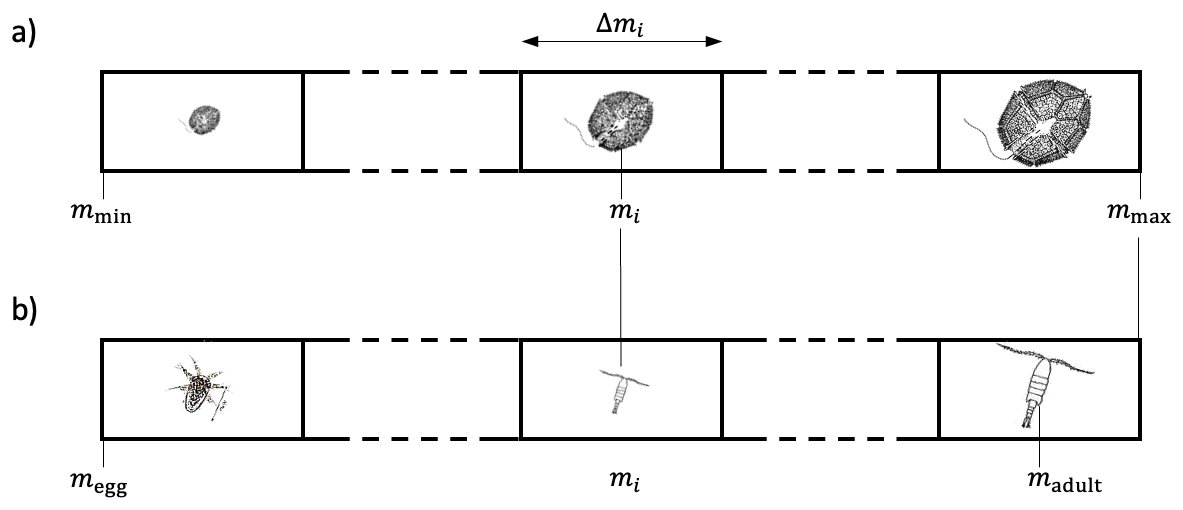
Figure A1 Specification of the computational grid used for unicellular organisms (a) and multicellular organisms (b). The grid for each unicellular plankton group (generalists and diatoms) contain n contiguous size groups in the range from m_min and m_max. Each size group is defined by its central mass (geometric mean) m_i. For multicellular plankton the grid for each group is from m_egg. The last size group has the central mass m_adult. This means that copepods actually becomes adult at smaller mass than m_adult, and that the last size group spans a range of masses.

Appendix B: Model equations and parameters

Equations and parameters for unicellular plankton are in Tables B1 and B2, for copepods in Tables B3 and B4, and parameters for POM in Table B5.

B1 Diatom membrane fraction

Let r be the radius of the entire cell including the outer membrane, r_vac the vacuole radius, ν_vac the fraction of the cell volume occupied by the vacuole, ρ the cell density, and δ the thickness of each membrane (see Fig. 2). The total cell volume is:

$$\begin{array}{}\text{(B1)}& V={\displaystyle \frac{\mathrm{4}}{\mathrm{3}}}\mathit{\pi }{r}^{\mathrm{3}}\iff r={\left({\displaystyle \frac{\mathrm{3}}{\mathrm{4}\mathit{\pi }}}V\right)}^{\mathrm{1}/\mathrm{3}}.\end{array}$$

The vacuole volume is:

$$\begin{array}{}\text{(B2)}& V_{\mathrm{vac}}={\displaystyle \frac{\mathrm{4}}{\mathrm{3}}}\mathit{\pi }{r}_{\mathrm{vac}}^{\mathrm{3}}\iff {\mathit{\nu }}_{\mathrm{vac}}{\displaystyle \frac{V_{\mathrm{vac}}}{V}}={\displaystyle \frac{r_{\mathrm{vac}}^{\mathrm{3}}}{r^{\mathrm{3}}}}\iff r_{\mathrm{vac}}=r{\mathit{\nu }}_{\mathrm{vac}}^{\mathrm{1}/\mathrm{3}}.\end{array}$$

The volume of the membranes is:

$$\begin{array}{}\text{(B3)}& V_{\mathrm{m}}=\underset{\mathrm{outer}\mathrm{membrane}}{\underbrace{{\displaystyle \frac{\mathrm{4}}{\mathrm{3}}}\mathit{\pi }\left(r^{\mathrm{3}}-(r-\mathit{\delta }{)}^{\mathrm{3}}\right)}}+\underset{\mathrm{inner}\mathrm{membrane}}{\underbrace{{\displaystyle \frac{\mathrm{4}}{\mathrm{3}}}\mathit{\pi }\left({\left(r_{\mathrm{vac}}+\mathit{\delta }\right)}^{\mathrm{3}}-r_{\mathrm{vac}}^{\mathrm{3}}\right)}}.\end{array}$$

The Taylor series expansion of $f\left(x\right)=r^{\mathrm{3}}-(r-x{)}^{\mathrm{3}}$ around δ=0 is 3r²δ.

The approximation for the volume of membranes is then:

$$\begin{array}{}\text{(B4)}& V_{\mathrm{m}}\approx \mathrm{4}\mathit{\pi }{r}^{\mathrm{2}}\mathit{\delta }+\mathrm{4}\mathit{\pi }{r}_{{\mathrm{vac}}^{\mathrm{2}}}\mathit{\delta }\stackrel{\left(\mathrm{B}\mathrm{2}\right)}{=}\mathrm{4}\mathit{\pi }\mathit{\delta }\left(\mathrm{1}+{\mathit{\nu }}_{\mathrm{vac}}^{\mathrm{2}/\mathrm{3}}\right)r^{\mathrm{2}}.\end{array}$$

Assuming the vacuole density to be 0, the mass of the cell is:

$$\begin{array}{}\text{(B5)}& \begin{array}{rl}m& =\mathit{\rho }\left(V-V_{\mathrm{vac}}\right)\stackrel{\left(\mathrm{B}\mathrm{2}\right)}{=}\mathit{\rho }V\left(\mathrm{1}-{\mathit{\nu }}_{\mathrm{vac}}\right)\\ & \iff r={\left({\displaystyle \frac{\mathrm{3}}{\mathrm{4}\mathit{\pi }}}{\displaystyle \frac{m}{\mathit{\rho }}}{\displaystyle \frac{\mathrm{1}}{\mathrm{1}-{\mathit{\nu }}_{\mathrm{vac}}}}\right)}^{\mathrm{1}/\mathrm{3}}.\end{array}\end{array}$$

The membrane fraction of the cell's mass is then:

$$\begin{array}{}\text{(B6)}& \begin{array}{rl}{\mathit{\nu }}_{\mathrm{m}}& ={\displaystyle \frac{\mathit{\rho }{V}_{\mathrm{m}}}{m}}\stackrel{(\mathrm{B}\mathrm{2},\mathrm{B}\mathrm{4})}{=}{\displaystyle \frac{\mathrm{4}\mathit{\pi }\mathit{\delta }\left(\mathrm{1}+{\mathit{\nu }}_{\mathrm{vac}}^{\mathrm{2}/\mathrm{3}}\right)r^{\mathrm{2}}}{\mathrm{4}/\mathrm{3}\mathit{\pi }\left(\mathrm{1}-{\mathit{\nu }}_{\mathrm{vac}}{r}^{\mathrm{3}}\right)}}\\ & =\mathrm{3}{\displaystyle \frac{\mathit{\delta }}{r}}{\displaystyle \frac{\mathrm{1}+{\mathit{\nu }}_{\mathrm{vac}}^{\mathrm{2}/\mathrm{3}}}{\mathrm{1}-{\mathit{\nu }}_{\mathrm{vac}}}}\stackrel{\left(\mathrm{B}\mathrm{5}\right)}{=}\mathrm{3}\mathit{\delta }{\left({\displaystyle \frac{\mathrm{4}\mathit{\pi }}{\mathrm{3}}}\right)}^{\mathrm{1}/\mathrm{3}}{\left({\displaystyle \frac{m}{\mathit{\rho }}}\right)}^{-\mathrm{1}/\mathrm{3}}\\ & {\displaystyle \frac{\mathrm{1}+{\mathit{\nu }}_{\mathrm{vac}}^{\mathrm{2}/\mathrm{3}}}{(\mathrm{1}-{\mathit{\nu }}_{\mathrm{vac}}{)}^{\mathrm{2}/\mathrm{3}}}}={\mathrm{6}}^{\mathrm{2}/\mathrm{3}}{\mathit{\pi }}^{\mathrm{1}/\mathrm{3}}\mathit{\delta }{\left({\displaystyle \frac{m}{\mathit{\rho }}}\right)}^{-\mathrm{1}/\mathrm{3}}{\displaystyle \frac{\mathrm{1}+{\mathit{\nu }}_{\mathrm{vac}}^{\mathrm{2}/\mathrm{3}}}{{\left(\mathrm{1}-{\mathit{\nu }}_{\mathrm{vac}}\right)}^{\mathrm{2}/\mathrm{3}}}}\end{array}\end{array}$$

and the active biomass fraction is: $\mathit{\nu }=\mathrm{1}-{\mathit{\nu }}_{\mathrm{m}}$.

Table B1 Equations for the unicellular models (generalists and diatoms).

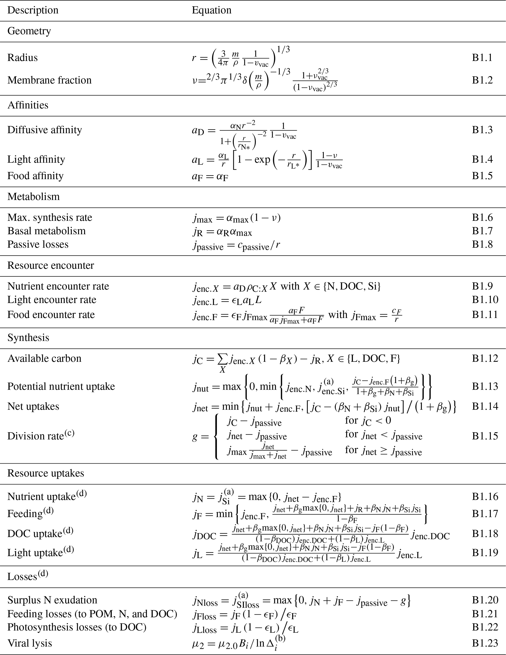
^(a) Only for diatoms. ^(b) Correction for the size-range of a size group where Δ_i is the ratio between the upper and lower sizes of a size group. ^(c) The three cases are: (1) when the available carbon j_C is less than the passive losses the cell experiences negative growth. (2) The same occurs if the net uptakes of nutrients and carbon is less than passive losses. In both these cases the uptakes are not limited by the functional response because there is no new biomass synthesis occurring. (3) This is the usual case where the net growth g is limited by the functional response. ^(d) The four last equations specify the down-regulated uptakes of carbon, food, and nutrients. The uptakes are less than or equal to the encounters in Eqs. (B1.9) to (B1.11). These uptakes enter into the main equations for each resource Eqs. (15)–(17) and into the predation mortality Eq. (3). ^(e) Losses occur due to exudation of surplus nutrients when uptake of carbon is insufficient to meet the demands of respiration, due to losses during the feeding process, due to losses photosynthesis, and mortality due to viral lysis.

Table B2 Parameters for the unicellular model (generalists and diatoms). All parameters from Andersen and Visser (2023) unless noted. Values in parentheses are for diatoms. Temperature corrections are given with Q₁₀ regulation (Eq. 18).

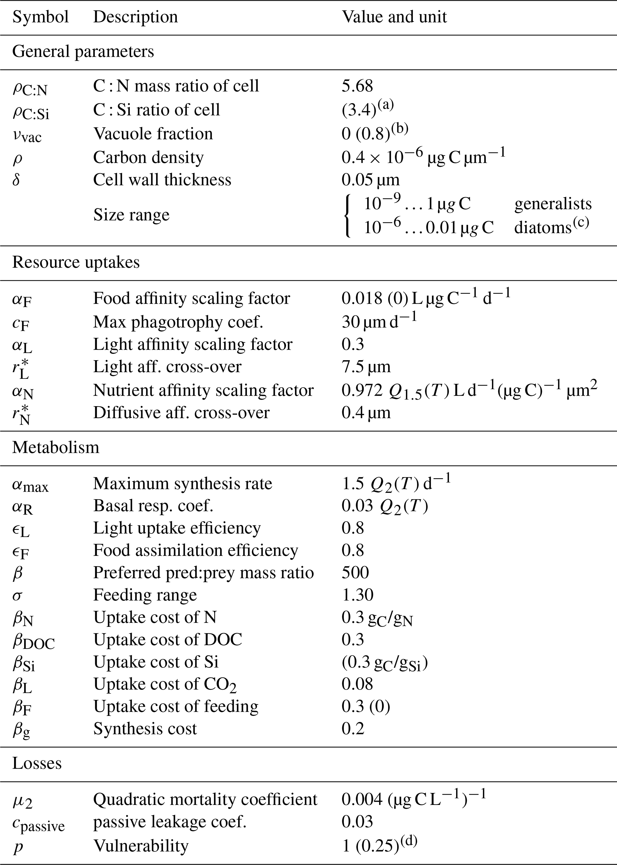
^(a) If the thickness of silicate shell of diatoms were independent of the size of the diatom, the Si : C ratio would decline with size. However, the thickness of the shell actually increases with size, probably to maintain the ability to withstand the crushing force of copepod mandibles (Pančić et al., 2019). Data shows that the C : Si ratio is roughly independent of size with an average value around 3.4 (Fig. B1b). ^(b) The vacule fraction increases slightly with size. Here we use a constant value of 0.8 which resonably well approximates date (Fig. B1a). ^(c) The size range of diatoms are roughly from $\mathrm{5}\times {\mathrm{10}}^{-\mathrm{6}}$ to 0.01 µg C (Pančić et al., 2019; Brzezinski, 1985). ^(d) The vulnerability parameter deteremines the diatom:phytoplankton ratio (Fig. E3). While we know that the vulnerability of diatoms to copepod predation varies with the thickness of the shell (Pančić et al., 2019) there is no laboratory information on the average relative vulnerability of diatoms relative to other relevant prey like dinoflagellates. Hence, the value of the vulnerability is rather arbitrarily set to 0.25.

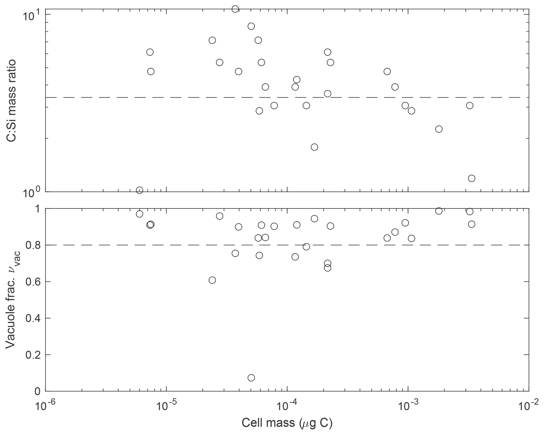
Figure B1 Analysis of diatom C : Si ratio (a) and vacuole fraction (b) as a function of carbon mass. The horizontal dashed lines show the values used in the diatom module. Data from Brzezinski (1985).

Table B3 Equations for the copepod growth and mortality model. Subscript “s” refers to the stage within the population and S is the adult stage. All variables are in dimensions of per time, except J_in which is biomass per time.

^(a) $m_{\mathrm{s}}^{-}/m_{\mathrm{s}}^{+}$ is the ratio between the lower and upper size of a size class; see Fig. A1.
^(b) The formulation of respiration is slightly revised from the original formulation in Serra-Pompei et al. (2020). It consists of two terms: a fixed basal respiration that is proportional to the maximum respiration and a “specific dynamics action” that is proportional to consumption.

Table B4 Parameters for the copepod model. All parameters are from Serra‐Pompei et al. (2022) except where noted.

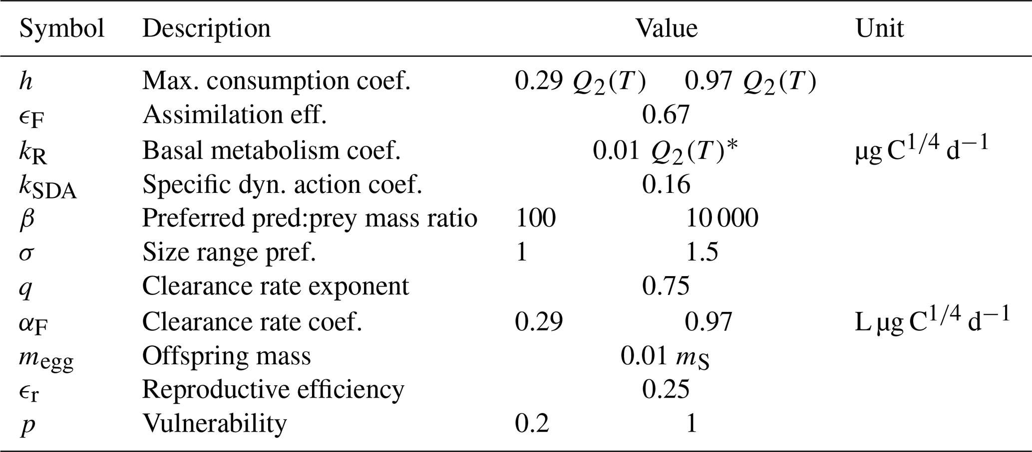
^* This value represents the starvation metabolism. Following Kiørboe et al. (1985) the starvation metabolism is approximately 18 % of the standard metabolism, which is approx. 20 % of max metabolism. This gives a very small value of k_R=0.006, which implies that copepods can survive a long time. We increase the value to k_R=0.01 such that large copepods can survive approx. 200 d which is sufficient to surve the winter at high latitudes.

Table B5 Parameters involved in POM and nutrient cycling.

Appendix C: Predation kernel

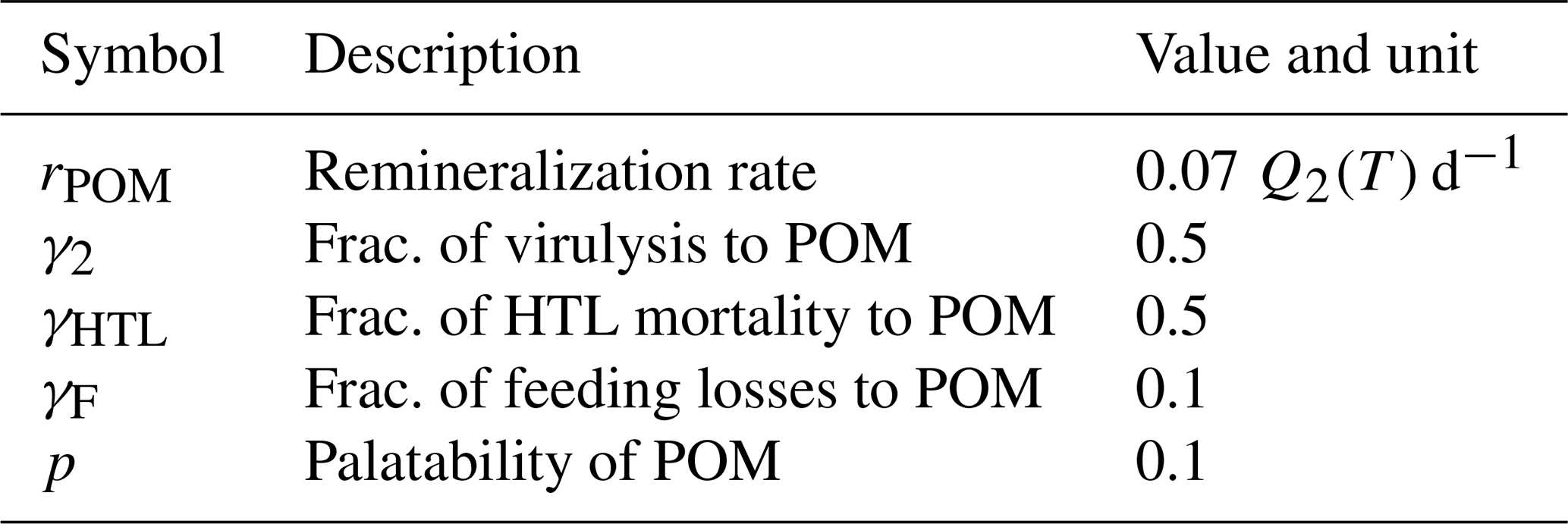
The effective prey preference function θ_ij between size classes of predators i and prey j should deal with the different width's of size classes depending on the size grid spacing. Following Andersen and Visser (2023) this is calculated by integrating over the prey size preference (Eq. 1). The encountered prey in size class j by all predators in class i is:

$$\begin{array}{}\text{(C1)}& E_{ij}=\underset{m_i^{-}}{\overset{m_i^{+}}{\int }}{a}_{\mathrm{F}}m\underset{m_j^{-}}{\overset{m_j^{+}}{\int }}\mathit{\varphi }(m,w)B\left(w\right)\mathrm{d}wB\left(m\right)/m\mathrm{d}m,\end{array}$$

where $m_i^{-}$ and $m_i^{+}$ represent the upper an lower bounds of size class i. B(m) represents the normalized biomass spectrum. We assume a Sheldon distribution, i.e., $B\left(m\right)\propto m^{-\mathrm{1}}$. With the discrete prey and predator groups we can write the encountered food as:

$$\begin{array}{}\text{(C2)}& E_{ij}=a_{\mathrm{F}}{m}_i{\mathit{\theta }}_{ij}{B}_j{N}_i\end{array}$$

where B_j is the total biomass in class j, $B_j=\int B\left(w\right)\mathrm{d}w$ and N_i is the total abundance of predators $N_i=\int B\left(m\right)/m\mathrm{d}m$. Equating the two terms and isolating θ_ij gives:

$$\begin{array}{}\text{(C3)}& \begin{array}{rl}{\mathit{\theta }}_{ij}& ={\displaystyle \frac{\sqrt{\mathrm{\Delta }}}{(\mathrm{\Delta }-\mathrm{1})\log \left(\mathrm{\Delta }\right)}}\left[\left({\displaystyle \frac{\mathrm{1}}{\mathrm{2}}}s\left(e^{-\frac{{\log }^{\mathrm{2}}\left(\frac{\mathrm{\Delta }z}{\mathit{\beta }}\right)}{s}}+e^{-\frac{{\log }^{\mathrm{2}}\left(\frac{\mathit{\beta }\mathrm{\Delta }}{z}\right)}{s}}\right.\right.\right.\\ & \left.-\mathrm{2}{e}^{-\frac{{\log }^{\mathrm{2}}\left(\frac{z}{\mathit{\beta }}\right)}{s}}\right)-{\displaystyle \frac{\mathrm{1}}{\mathrm{2}}}\sqrt{\mathit{\pi }}\sqrt{s}\left(\log \left({\displaystyle \frac{\mathrm{\Delta }z}{\mathit{\beta }}}\right)\mathrm{erf}\right.\\ & \left({\displaystyle \frac{\log \left(\mathit{\beta }\right)-\log \left(\mathrm{\Delta }z\right)}{\sqrt{s}}}\right)+\log \left({\displaystyle \frac{\mathit{\beta }\mathrm{\Delta }}{z}}\right)\mathrm{erf}\\ & \left.\left.\left.\left({\displaystyle \frac{\log \left(z\right)-\log \left(\mathit{\beta }\mathrm{\Delta }\right)}{\sqrt{s}}}\right)+\log \left({\displaystyle \frac{z}{\mathit{\beta }}}\right)\mathrm{erf}\left({\displaystyle \frac{\log \left(\frac{z}{\mathit{\beta }}\right)}{\sqrt{s}}}\right)\right)\right)\right]\end{array}\end{array}$$

where s=2σ² and $z=m_i/m_j$ and $\mathrm{\Delta }=m^{+}/m^{-}$. In this way θ_ij represent the total preference of size class i and j, including a compensation for the width of size classes and the preference p_kl between predator from group k on group l (from Eq. 1). Technically the preference should be expressed as θ_klij, where k and l are the indices of predation and prey functional group, but the dependence on the group preferences is suppressed to improve readability.

Appendix D: Data sources and processing

D1 POC biomass: GOPOPCORN

GO-POPCORN v2 consists of samples from 12 cruises from 2011 to 2020. We used POCavg_uM that range between 0.7 and 30 µm. We compare the POC data with all plankton and detritus particles with a radius between 0.35–15 µm at the same coordinates, month and depth.

D2 Picophytoplankton biomass

We export the in situ phytoplankton biomass (Prochlorococcus, Synechococcus and Picoeukaryotic) at different transects and chlorophyll-a (depth-averaged between 0–10 m and ignoring the deeper samples to match satellite measurements), that where measured at different months (ref. “Intercomparison of Ocean Color Algorithms from Picophytoplankton Carbon in the Ocean”). The cell counts were from water samples from up to 200m depth, between 1997 and 2014. In situ data are compared to the models output at the top layer.

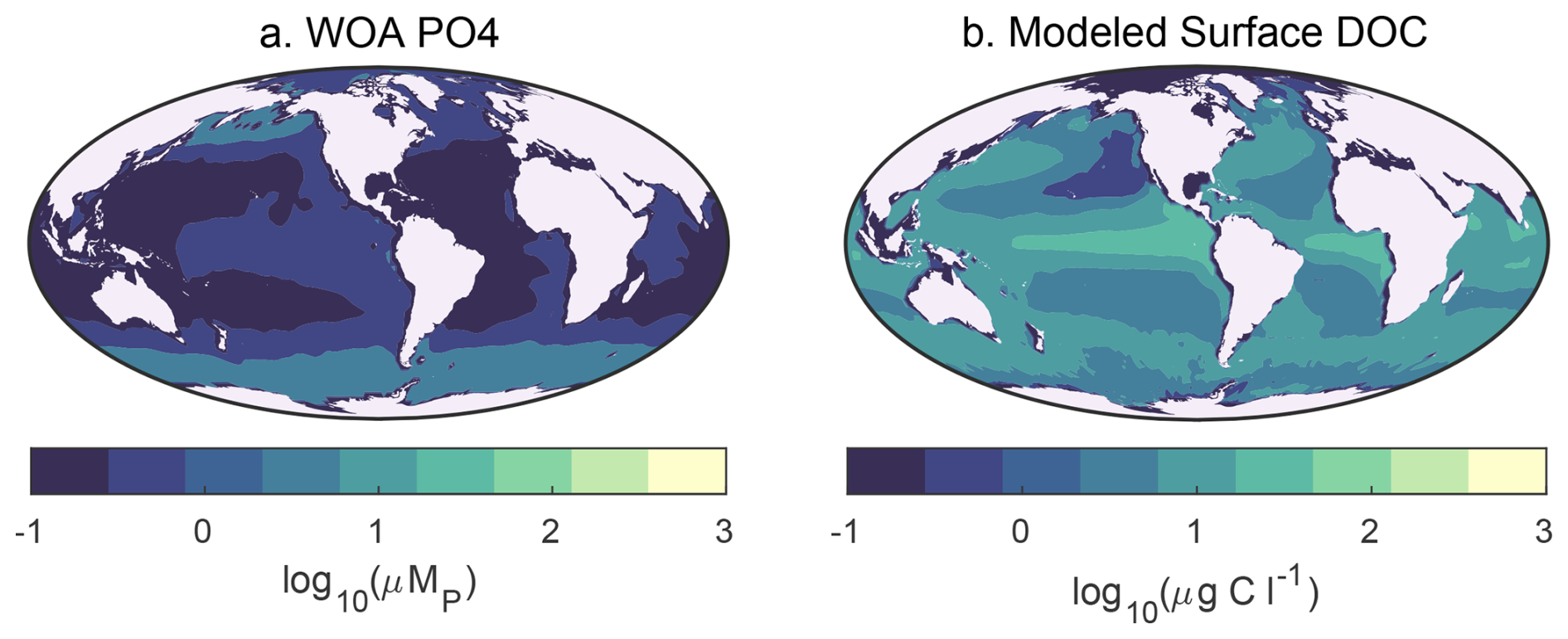
Figure D1 Annual mean concentrations of (a) phosphate (µg P L⁻¹) from World Ocean Atlas (Reagan et al., 2023) and (b) dissolved organic carbon (µg Si L⁻¹) at top 5 m.

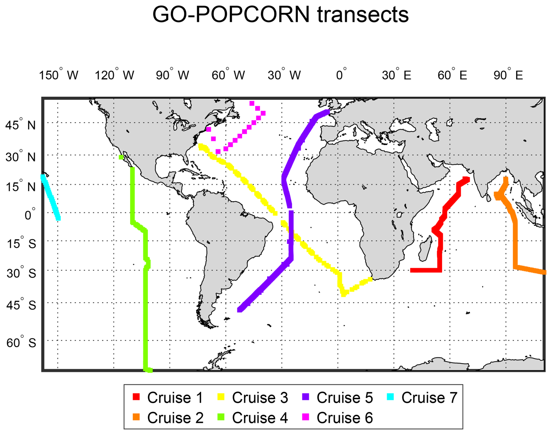
Figure D2 GOPOPCORN Cruises transects.

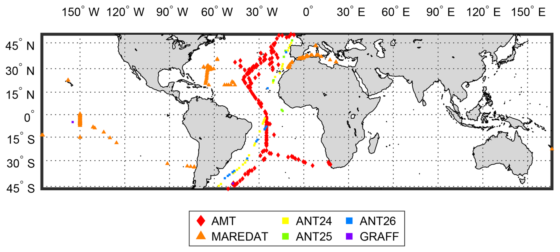
Figure D3 Picophytoplankton Cruises from Martínez-Vicente et al. (2017b).

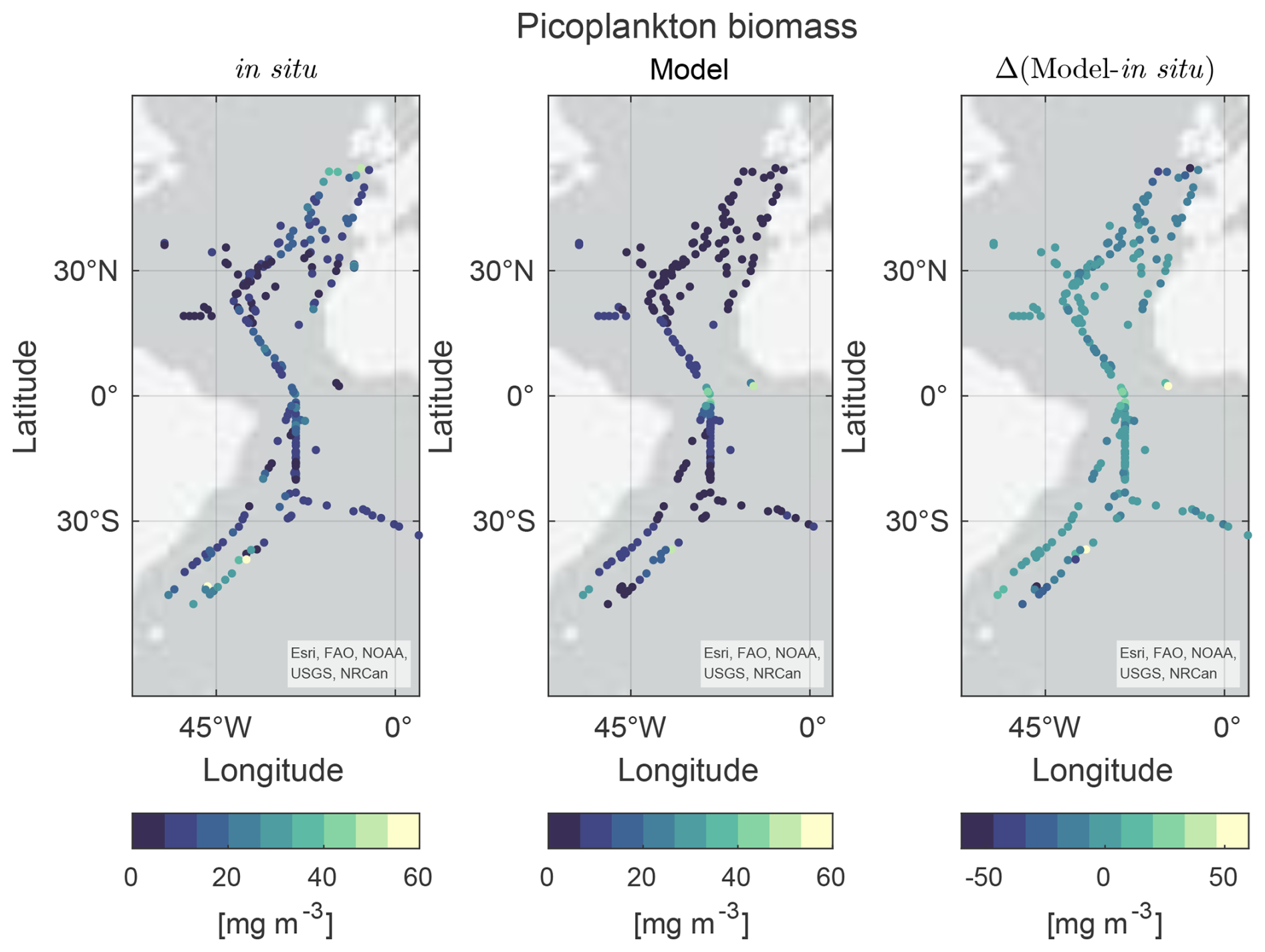
Figure D4 Comparison of picophytoplankton in situ data (Martínez-Vicente et al., 2017b) with model picoplankton biomass. Basemap: Esri, FAO, NOAA, USGS, NRCan; powered by Esri.

Appendix E: Additional figures

Figure E1 Model output for a 10-year simulation in the global, water column and chemostat model. (a) Total biomass in a water column extracted from the global simulation from Fig. 7 at an upwelling location (5° S, 5° E). (c) Same as (a) but extracted from the watercolumn model. (b, d, e) Sheldon spectrum of the community from global, water column and chemostat models at 5 meters depth and averaged over the last year.

Figure E2 Same as in Fig. E1, but at an oligotrophic location (24° N, 158° W).

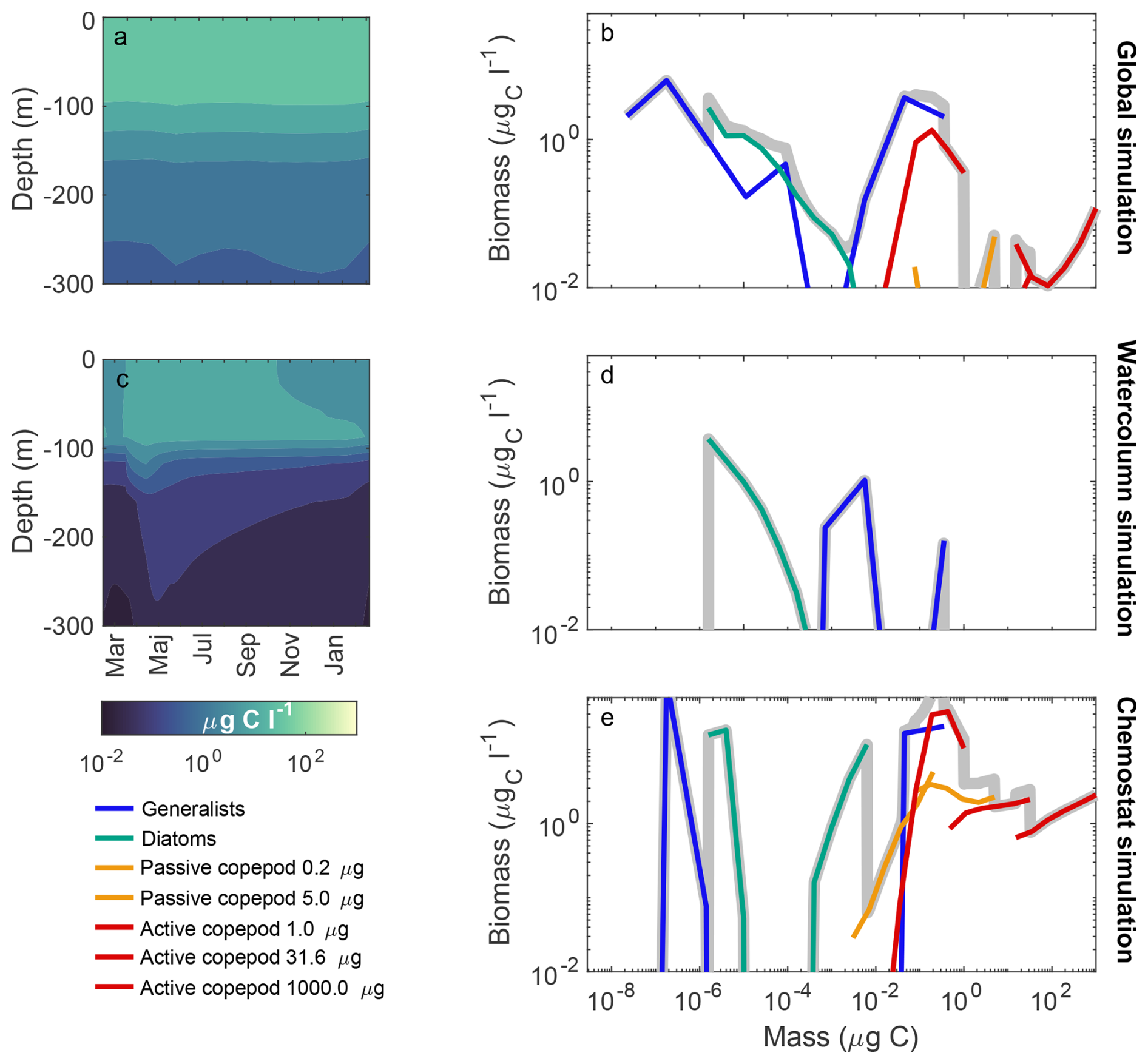
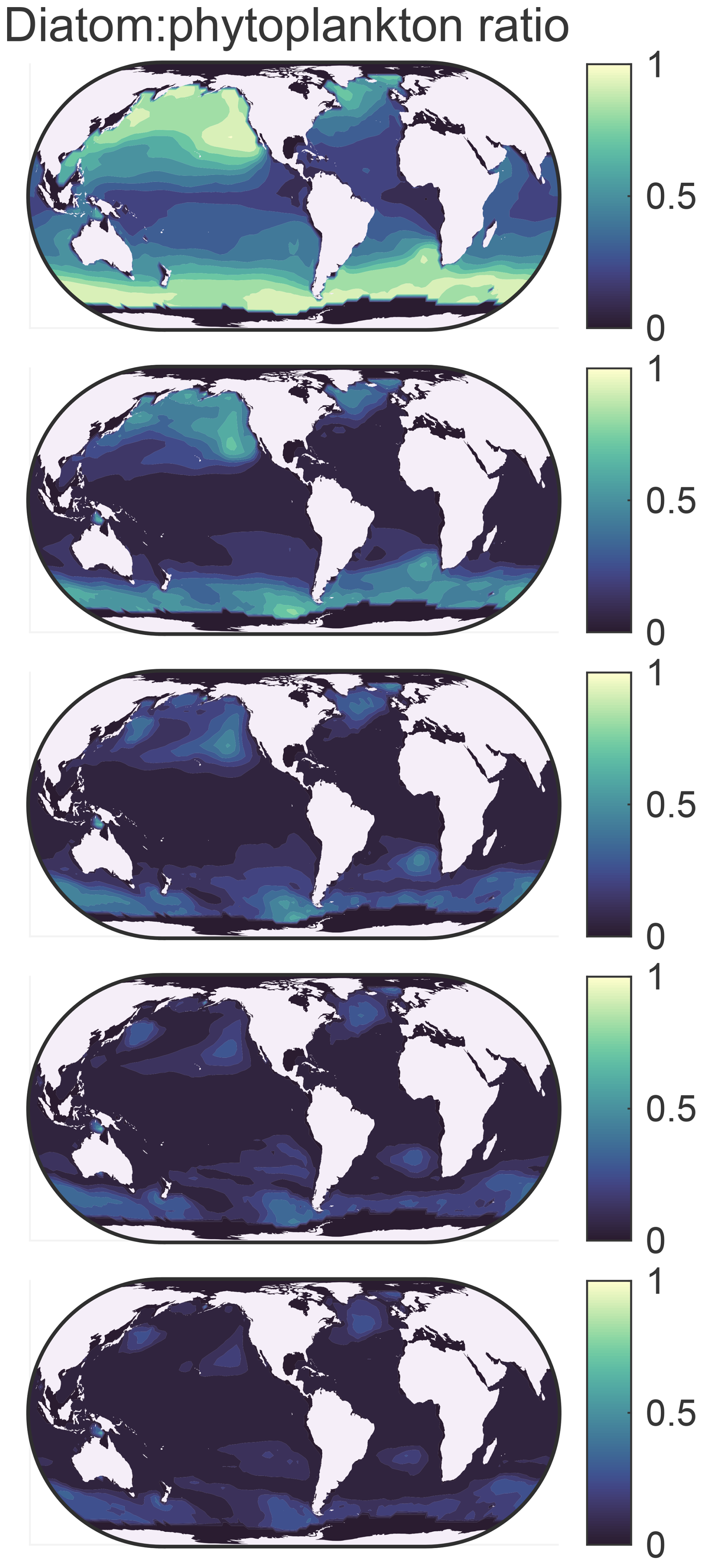
Figure E3 Annual mean surface diatom:phytoplankton ratio for values of the diatom vulnerability ranging from 0 (top) to 1 (bottom).

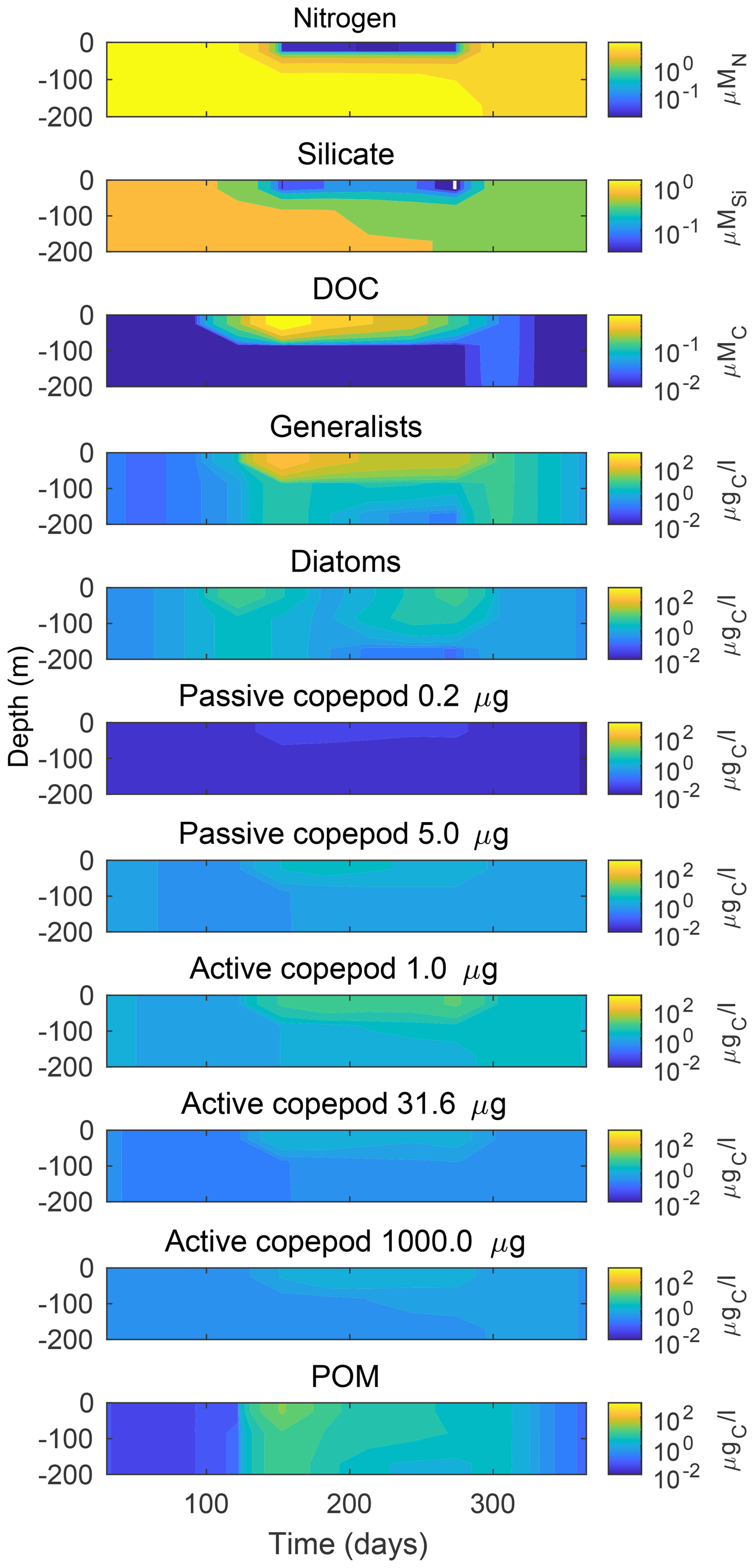
Figure E4 Output of a water-column simulation corresponding to Fig. 15c: (from top to bottom) (a) surface nitrogen (µg${}_{\mathrm{N}}/l$), (b) silicate (µg_Si L⁻¹), and (c) DOC (µg_C L⁻¹); (d) total generalist biomass (µg_C m⁻²), (e) diatom biomass, (f) passive copepod 0.2 µg_C, (g) passive copepod 5 µg_C, (h) active copepod 1.0 µg_C, (i) active copepod 10 µg_C, (j) active copepod 100 µg_C, (k) active copepod 1000 µg_C, and (l) POM.

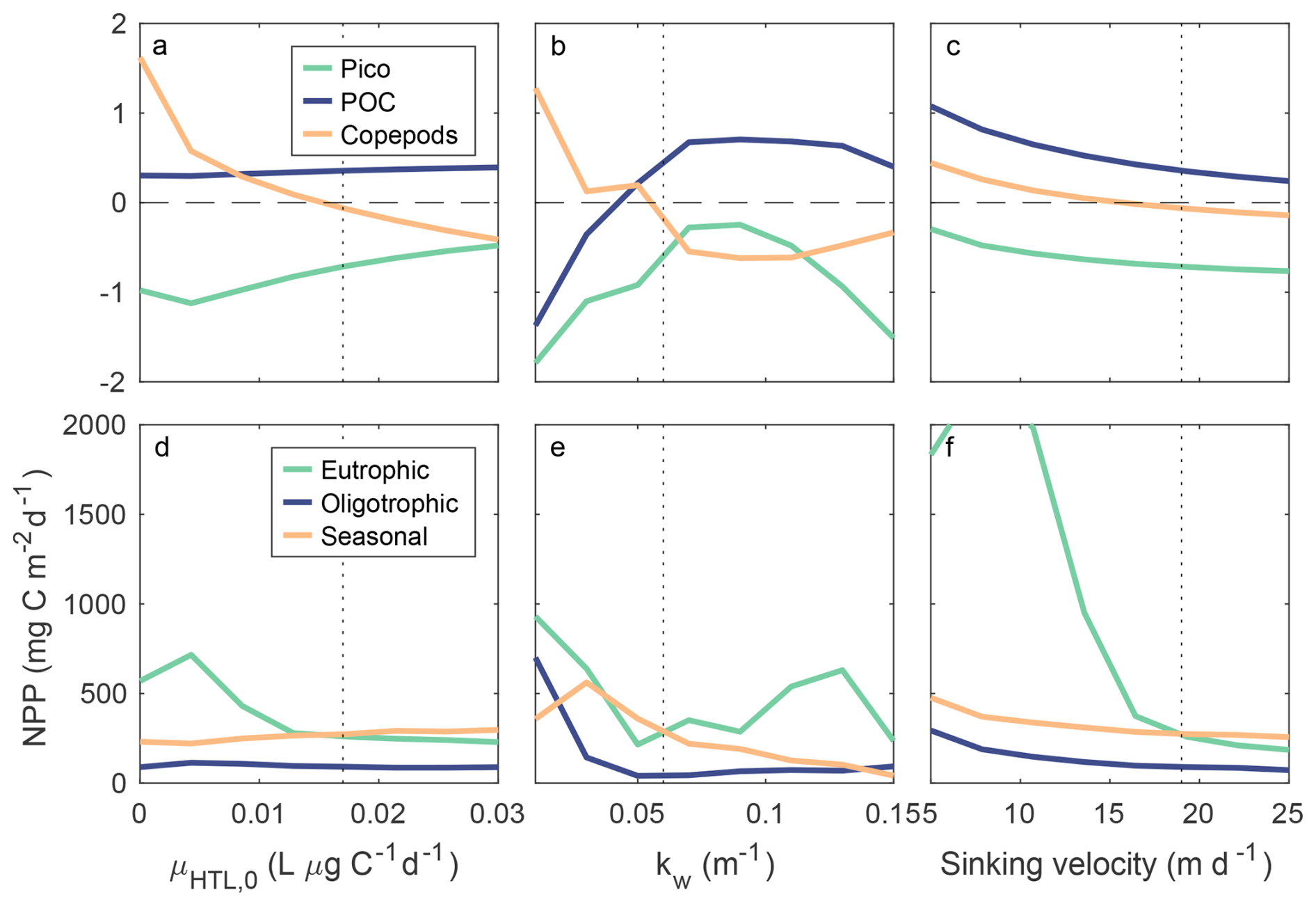
Figure E5 Sensitivity analysis of the parameters: higher trophic level mortality μ_HTL, light extinction coefficient k_w, and sinking velocity u. (a–c) The objective function for comparison with pico-plankton, POC, and copepods (see Fig. 6. (d–f) NPP at three characteristic water columns extracted from global simulations.

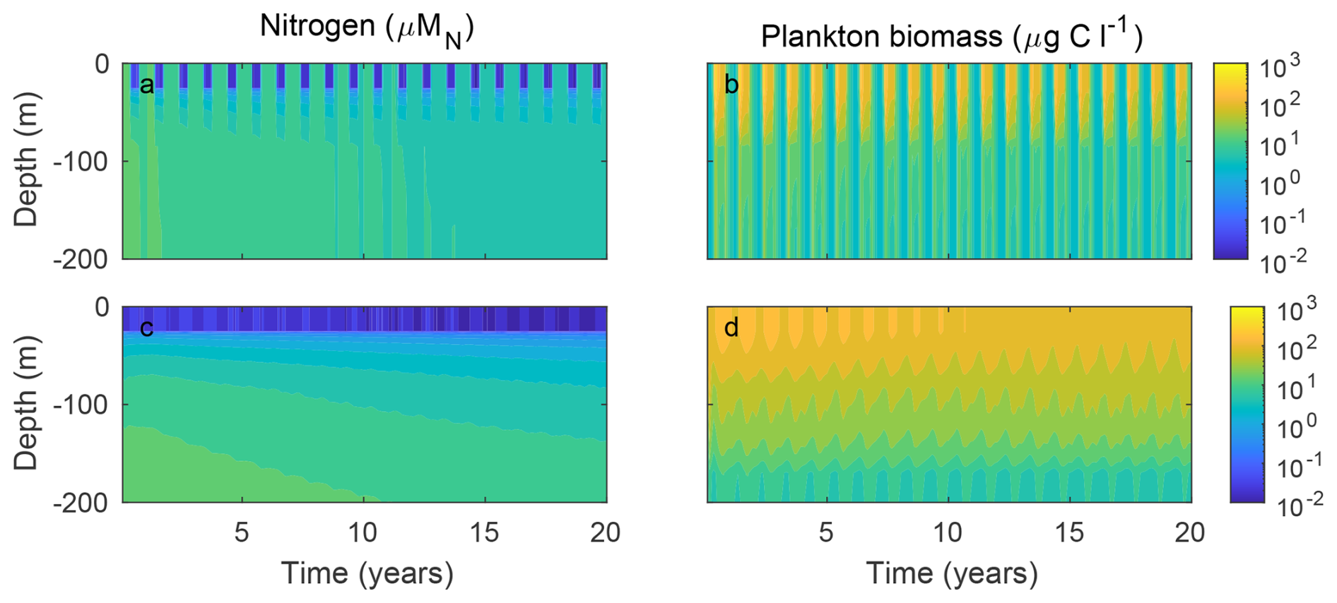
Figure E6 Convergence of a global simulation in a seasonal environment (60° N, 40° W; a, b) and at equator (0° N, 15° W; c, d).

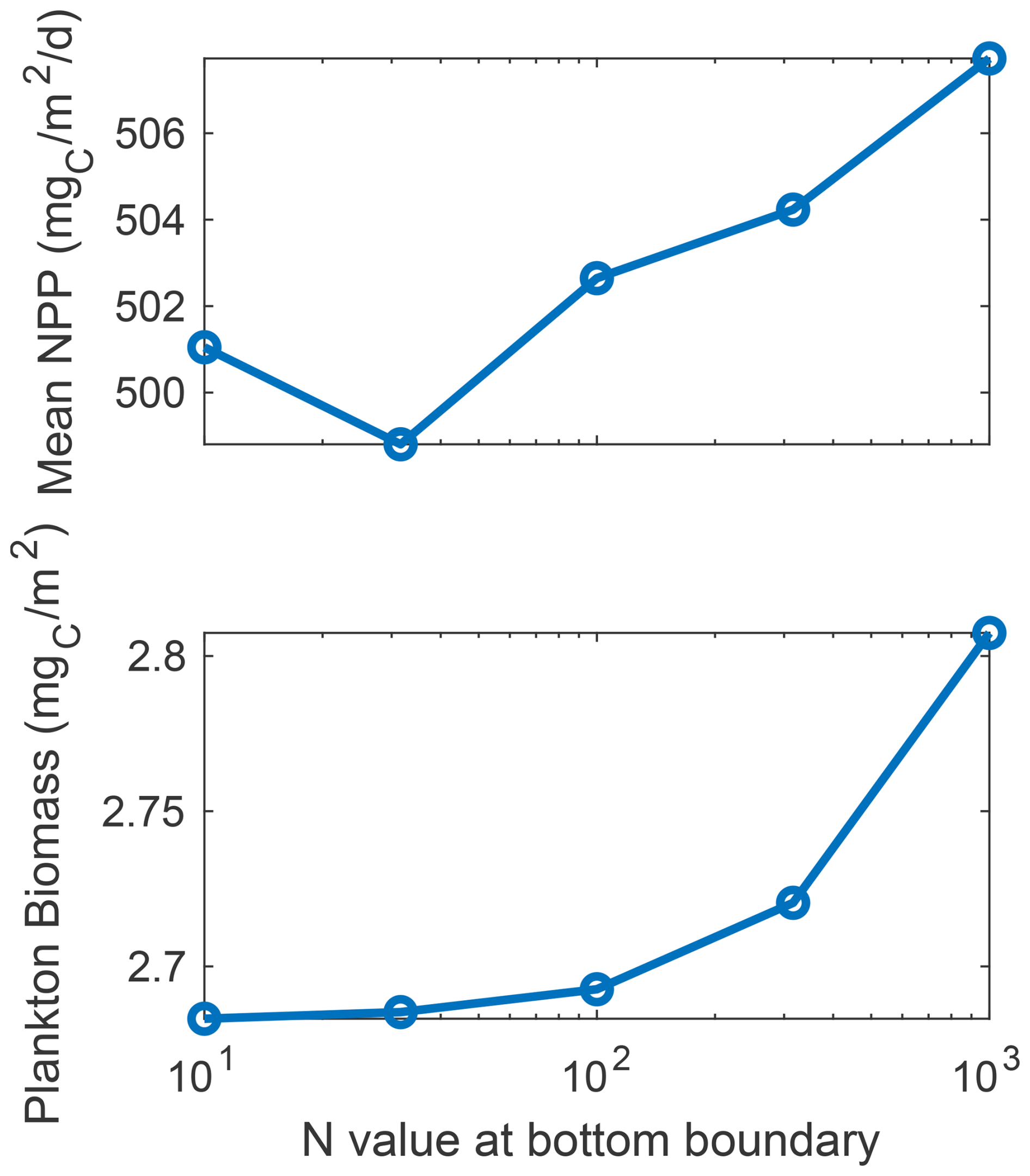
Figure E7 Exploration of the influence of the bottom condition on nutrient on net primary production (top panel) and plankton biomass (bottom panel). The values are the last year from a 10 year simulation of a seasonal water column at 60° N and 40° W.