Cleo: the numerical methods of a new superdroplet model including a droplet breakup algorithm (v0.52.0)

The numerical methods of Eulerian bulk and bin models have obscured our fundamental understanding of cloud microphysics and introduced artificial uncertainties. In contrast, the Super-Droplet Method (SDM) provides a transparent link between model and theory, and remedies the numerical artifacts that hindered decades of cloud modelling. In light of its numerous advantages we've created a novel SDM for warm-cloud microphysics called Cleo, with the goal of making it feasible to run Large-Eddy Simulations (LES) with SDM in domains large enough to resolve shallow mesoscale cloud organisation 𝒪(100 km). Here we document the microphysics grounding Cleo and how it is translated into numerical methods, with the intention of assisting the physical interpretation of future LES and comparison with observations. We highlight subtle but important points where we differ from existing SDMs: in how we model the ventilation effect on evaporation, and how we account for uncertainty in our knowledge of droplet collisions. As well as modelling collision-coalescence, we propose a low-cost extension to the original SDM algorithm which adds both collisional rebound and breakup. We demonstrate Cleo's capabilities with known test-cases for condensation/evaporation, collisions between droplets, and droplet motion, including an integrated test using the 1-D Kinematic Driver framework. Cleo can therefore now be used stand-alone, one-way coupled for piggybacking, or two-way coupled for LES, as a fully-functioning SDM capable of representing all the main microphysical processes driving warm-clouds.

1 Introduction

Substantial differences exist between conventional Eulerian models for cloud microphysics. Excessive degrees of freedom within one- and two-moment bulk schemes, the least expensive of existing microphysics models, allow for varying definitions of condensate categories, as well as the parametrisations for how they interact with one another, and their assumed size distributions (Khain et al., 2015). Increasing in sophistication, even the most conventional spectral bin schemes still vary in how they define condensate categories and their parametrisations. They also introduce differences in numerical implementations, for example to tackle numerical diffusion (Morrison et al., 2020), such that even if two bin schemes solve the same equations they could calculate different results. These differences matter for more than just microphysics.

The differences between conventional Eulerian, bulk and bin, models have a wide-range of macrophysical ramifications. In global storm resolving models (e.g. Miyakawa et al., 2014; Bretherton, 2015), only changing fall velocity parameters in one- and two- moment bulk schemes can substantially alter the relationship between moisture and convection, which has consequences for the Madden–Julian oscillation and the radiation balance of the entire atmosphere (Suematsu et al., 2021; Takasuka et al., 2024; Naumann et al., 2025). Varying definitions of condensate size distributions in bulk schemes are also problematic because they alter shallow-cloud fraction and albedo, even in non-precipitating clouds, and their underlying assumptions, regarding the functional form of each distribution and distinguishing between “rain” and “cloud” condensates, are known to be inconsistent with observations and with bin scheme models of cloud microphysical processes (e.g. Igel and van den Heever, 2017a, b; Igel, 2019; Igel et al., 2022). When Large-Eddy Simulations (LES) and observations are compared, differing precipitation patterns are frequently attributed to differences in microphysics schemes (e.g. Ackerman et al., 2009; King et al., 2015; Schulz and Stevens, 2023), and bin schemes have been shown to be just as disparate as bulk ones (vanZanten et al., 2011; Hu and Igel, 2023; Hill et al., 2023). Indeed there is extensive literature showing the many ways in which microphysics can appreciably affect larger-scale dynamics (e.g. Barnes and Garstang, 1982; Hagos et al., 2018; Jian et al., 2021; Gasparini et al., 2023), and thus as long as there are differences between microphysics schemes we can expect there to be differences in macrophysical outcomes. Differences inevitably arise from gaps in our knowledge of cloud microphysics, however, the differences highlighted above are not caused by knowledge gaps, but rather by “model uncertainty”, uncertainty inherent to the way that conventional Eulerian cloud microphysics models represent what we already understand (Grabowski et al., 2019; Morrison et al., 2020).

The Super-Droplet Method (SDM; Shima et al., 2009) is a Lagrangian particle method for modelling cloud microphysics where the condensate population is represented by “superdroplets”. Superdroplets have the same properties as real condensates as well as an extra one, the multiplicity, which states how many real condensate particles that superdroplet stands for. In a somewhat analogous way to bulk schemes where the accuracy of the condensate size distributions is bounded by the number of moments, and to bin schemes where it is bounded by the number of bins, it is the number of superdroplets which limit the accuracy of SDM. The major limitation of SDM is its computational cost, both in terms of its memory consumption and its number of computations, which presumably is the reason that LES using SDM have so far been limited to domains 𝒪(10 km) or smaller (to the best of our knowledge, the largest LES with SDM to-date are Sato et al., 2017; Chandrakar et al., 2021; Matsushima et al., 2023 and Yin et al., 2024). Historically, Lagrangian particle-based microphysics schemes have struggled computationally (e.g. Jacobson, 2005; Simmel and Wurzler, 2006) whilst bin and bulk schemes have advanced not only cloud process understanding but also numerical weather and climate prediction in ways that would not otherwise have been possible, by working within the computational constraints of the time (Khain et al., 2015; Morrison et al., 2020). Nevertheless, advances in high-performance computing combined with SDM's embarrassingly parallel algorithms, make SDM a promising model for cloud microphysics on current and upcoming computer architectures (Shima et al., 2009; Grabowski et al., 2019; Morrison et al., 2020; Matsushima et al., 2023), potentially changing the perception that Lagrangian particle-based cloud microphysics is too computationally expensive.

Part of what makes SDM appealing is that SDM eradicates the biggest sources of conventional model uncertainty. Whilst SDM is not free of modelling assumptions and hence still suffers from its own sources of model uncertainty (Hill et al., 2023), SDM makes no assumptions about condensate categories or size distributions unlike bulk schemes, and it does not suffer from same intrinsic problems as bin schemes, such as numerical diffusion and the “curse of dimensionality” (Grabowski et al., 2019). Furthermore, SDM has an important convergence property. As the number of superdroplets increases, a simulation tends towards what we expect from explicit individual particle simulations (Shima et al., 2009), and the mean of many simulations of its collision-coalescence algorithm approaches the solution to the Smoluchowski equation (Smoluchowski, 1916). This is in stark contrast to bulk schemes, where increasing refinement does not converge to a generic solution, and also to bin schemes which model collisions by solving the Smoluchowski equation directly. Bulk schemes therefore suffer from the limitations of that equation; namely its mean-field approximation assumes that the locations of differently sized droplets are uncorrelated (Gillespie, 1972), even though this is only variably true (Dziekan and Pawlowska, 2017; Morrison et al., 2020), and prevents modelling “lucky drops” which may be crucial for precipitation onset (Telford, 1955; Kostinski and Shaw, 2005; Dziekan and Pawlowska, 2017; Morrison et al., 2020). In SDM, the stochastic collision-coalescence algorithm does not make these assumptions and can represent lucky drops (Dziekan and Pawlowska, 2017; Li et al., 2022). Finally, the link between our fundamental (particle-based) understanding of microphysical processes and their representation in SDM is clearer and more direct than in Eulerian microphysics models, meaning that variations between SDMs hold a stronger relation to differences in our understanding of the underlying physics.

We have created a novel computational implementation of SDM, Cleo. Our goal is to make a simplistic, ordinary representation of warm-cloud microphysics according to SDM which is well-suited to high-performance computers. Consequently we hope to make SDM feasible for large-enough-domain LES to resolve the interactions between warm-cloud microphysics and shallow mesoscale cloud organisation 𝒪(100 km). In the companion to this paper we described the fundamental computational design of our SDM and its computational performance (Bayley et al., 2026). In this paper we document Cleo's numerical methods for warm-cloud microphysics and demonstrate their behaviour in known test-cases. Since the link between the numerical methods and fundamental theory is so clear in SDM, by carefully describing our numerical methods we assist the physical interpretation of studies using Cleo and comparisons with other microphysics models.

Cleo models all the major microphysical processes of warm-clouds: condensation/evaporation, collisions between droplets and droplet motion. Most of the methods are already found in the literature, but in addition to documenting which of those Cleo adopts, we highlight particular novelties of our approaches and explain how the flexibility we incorporated reflects the uncertainties in our current understanding of warm-cloud microphysics. More specifically, we clarify the methods of Shima et al. (2009) and Matsushima et al. (2023) for modelling condensation/evaporation and extend them to include ventilation effects. For collision between droplets, Cleo can use the original collision-coalescence algorithm according to Shima et al. (2009), however Cleo also facilitates various definitions for the collision kernel and the outcome of collisions between droplets. The breakup of raindrops as a consequence of collisions is included in de Jong et al. (2023a) and Bringi et al. (2020), but is neglected by the majority of SDMs (and some bulk and bin microphysics schemes), despite the fact it could be an important influence on the rate of evaporation in downdraughts (Stevens and Seifert, 2008; Morrison and Milbrandt, 2011; Morrison et al., 2012; Seifert and Heus, 2013; Planche et al., 2019). Cleo therefore offers an extended version of the Shima et al. (2009) collision-coalescence algorithm to permit the study of rebound and breakup.

In this paper the ith superdroplet is defined by its spatial coordinates, x_i, its multiplicity, ξ_i, and its attributes, a_i, wherein R_i and M_s,i are its radius and its mass of solute (aerosol), respectively. The total mass of each superdroplet is given by

$$\begin{array}{}\text{(1)}& M_{\mathrm{T},i}=M_{\mathrm{s},i}\left(\mathrm{1}-{\displaystyle \frac{{\mathit{\rho }}_{\mathrm{l}}}{{\mathit{\rho }}_{\mathrm{s},i}}}\right)+{\displaystyle \frac{\mathrm{4}}{\mathrm{3}}}\mathit{\pi }{\mathit{\rho }}_{\mathrm{l}}{R}_i^{\mathrm{3}},\end{array}$$

to account for the solute's volume whilst neglecting its change due to dissolution, where ρ_l and ρ_s,i are the densities of liquid water and the solute, respectively. ${{\mathit{a}}^{\prime }}_i$ symbolises x_i as well as all the superdroplet's intensive attributes, for example ρ_s,i.

Cleo's numerical methods for microphysics and droplet motion are found in Sects. 2 to 4; Sect. 5 details how Cleo couples to a host dynamical driver; and the verifications of Cleo's numerical methods are found in Sect. 6. Within Sects. 2 to 4, Sect. 2 describes how Cleo models condensation/evaporation, including ventilation effects and an adaptive sub-time-stepping algorithm; Sect. 3 explains how we have extended the collision-coalescence algorithm of Shima et al. (2009) to include a framework for collisional breakup and rebound; and Sect. 4 explains how Cleo determines (super-)droplet motion.

2 Condensation/Evaporation

We use Köhler theory to describe droplet growth due to evaporation/condensation, but also account for the enhancement of evaporation of moving droplets by including a ventilation factor. The change of the ith superdroplet's radius, R_i, is therefore

$$\begin{array}{}\text{(2)}& R_i{\displaystyle \frac{\mathrm{d}{R}_i}{\mathrm{d}t}}=f_{\mathrm{v}}{\displaystyle \frac{(S-\mathrm{1})-\frac{a}{R_i}+\frac{b}{R_i^{\mathrm{3}}}}{F_k+F_{\mathrm{d}}}},\end{array}$$

where f_v is the ventilation factor; S is the ambient saturation ratio of the grid-box; F_k and F_d are, respectively, the heat conductivity and vapour diffusion factors; $\frac{a}{R_i}$ represents the effect of curvature on the saturation at a droplet's surface; and $\frac{b}{R_i^{\mathrm{3}}}$ accounts for the reduction in water vapour pressure due to the presence of solute. We use the same formulations for F_k, F_d, a and b as in Shima et al. (2009) (Köhler, 1936; Rogers and Yau, 1989). Supersaturation fluctuations caused by sub-grid-scale turbulence are not taken into account.

We obtain the ventilation factor, f_v, by fitting the curve

$$\begin{array}{}\text{(3)}& f_{\mathrm{v}}\left(R\right)=\mathrm{1}+{\left({\displaystyle \frac{\mathrm{1}}{{\mathit{\alpha }}_{\mathrm{1}}{R}^{{\mathit{\beta }}_{\mathrm{1}}}}}+{\displaystyle \frac{\mathrm{1}}{{\mathit{\alpha }}_{\mathrm{2}}{R}^{{\mathit{\beta }}_{\mathrm{2}}}}}\right)}^{-\mathrm{1}}\end{array}$$

to the curve from Pruppacher and Klett (1978), such that ${\mathit{\alpha }}_{\mathrm{1}}=\mathrm{6.954}\times {\mathrm{10}}^{\mathrm{7}}$ ${\mathrm{m}}^{-{\mathit{\beta }}_{\mathrm{1}}}$, ${\mathit{\alpha }}_{\mathrm{2}}=\mathrm{1.069}\times {\mathrm{10}}^{\mathrm{3}}$ ${\mathrm{m}}^{-{\mathit{\beta }}_{\mathrm{2}}}$, β₁=1.963, β₂=0.702. This gives similar values as Pruppacher and Klett (1978) (given the terminal velocity parametrisation from Pruppacher and Klett, 1978) but makes the size dependence more explicit whilst neglecting the small dependence of f_v on pressure variations. Additionally we constrain f_v≤20.0 to reflect the fact that droplets with a radius larger than approximately 3 mm have the same terminal velocity (see also Fig. 6). As shown in Fig. 1, f_v is negligible for droplets with radii less than about 0.1 mm, but can increase the evaporation rate of large droplets by an order of magnitude.

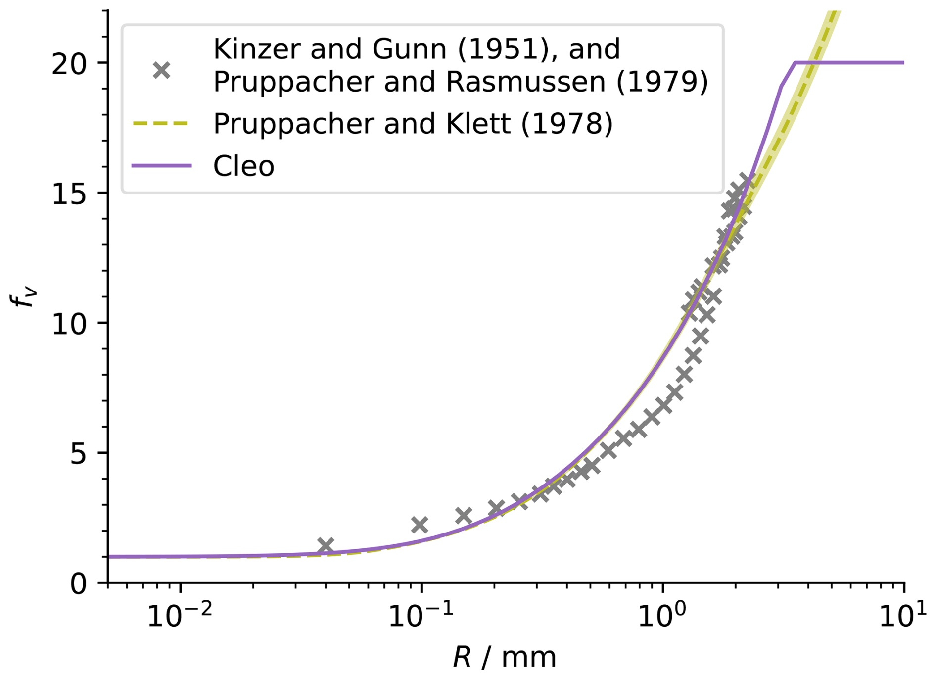
Figure 1 The ventilation factor we use in Cleo compared to the experimental data from Kinzer and Gunn (1951), and Pruppacher and Rasmussen (1979), and compared to the fit to the data from Pruppacher and Klett (1978) at $T=(\mathrm{288.15}\pm \mathrm{15.00})\mathrm{K}$ in a standard atmosphere.

Careful consideration of the numerical methods for integrating Eq. (2) is required because this ordinary differential equation is stiff. We use an implicit Euler method with a Newton-Raphson root-finding algorithm similar to Shima et al. (2009) to ensure stability when integrating the modified version of the ODE in Eq. (2). Our method saves computational cost by permitting a comparatively large default time-step (Δt_cond∼1 s) and very often keeping the number of Newton-Raphson iterations below three. Explicitly, given the time-step for condensation/evaporation, Δt_cond, and the notation $R_i\left(t^n\right)=R_i^n$, we make the approximation $f_{\mathrm{v}}\left(R\right)\approx f_{\mathrm{v}}\left(R_i^n\right)$ and let $f_{\mathrm{v}}\left(R_i^n\right)=f_{\mathrm{v}}$, the ODE is discretised as

$$\begin{array}{}\text{(4)}& \mathrm{0}={\displaystyle \frac{Z-(R_i^n{)}^{\mathrm{2}}}{\mathrm{\Delta }{t}_{\mathrm{cond}}}}-{\displaystyle \frac{\mathrm{2}{f}_{\mathrm{v}}\left[\right(S-\mathrm{1})-a{Z}^{-\mathrm{1}/\mathrm{2}}+b{Z}^{-\mathrm{3}/\mathrm{2}}]}{F_k+F_{\mathrm{d}}}};\end{array}$$

where $Z=(R_i^{n+\mathrm{1}}{)}^{\mathrm{2}}$. The Newton-Raphson method is then used to find the real positive root of the polynomial,

$$\begin{array}{}\text{(5)}& g\left(Z\right)={\displaystyle \frac{Z-(R_i^n{)}^{\mathrm{2}}}{\mathrm{\Delta }{t}_{\mathrm{cond}}}}-{\displaystyle \frac{\mathrm{2}{f}_{\mathrm{v}}\left[\right(S-\mathrm{1})-a{Z}^{-\mathrm{1}/\mathrm{2}}+b{Z}^{-\mathrm{3}/\mathrm{2}}]}{F_k+F_{\mathrm{d}}}};\end{array}$$

such that the radius of each superdroplet at the subsequent time-step is given by $R_i^{n+\mathrm{1}}=+\sqrt{Z}$ when g(Z)=0. We use g(Z) rather than the higher order polynomial in terms of $+\sqrt{Z}$ because it converges more rapidly – in fact in the limit $a=b=\mathrm{0}$, the Newton-Raphson method can find the true root of Eq. (5) with one iteration. A reasonable initial guess close to the true solution for g(Z)=0 can make convergence fast and so we choose our first guess for Z to be $(R_i^n{)}^{\mathrm{2}}$ unless $S>\mathrm{1}+\sqrt{\frac{\mathrm{4}{a}^{\mathrm{3}}}{\mathrm{27}b}}$, in which case the superdroplet is already activated and we make the initial guess very large: at least 10⁻⁶ m².

There are up to three real roots of g(Z) and so we must ensure that the genuine solution for $R_i^{n+\mathrm{1}}$ is converged upon. If the droplet was previously and is currently un-activated, and in an environment with a supersaturation less than its activation supersaturation, i.e. if

$$\begin{array}{}\text{(6)}& S\le \mathrm{1}+\sqrt{{\displaystyle \frac{\mathrm{4}{a}^{\mathrm{3}}}{\mathrm{27}b}}},\text{and}{R}_i^n<\sqrt{{\displaystyle \frac{\mathrm{3}b}{a}}},\end{array}$$

then the uniqueness of the solution to g(Z)=0 is guaranteed. Likewise, if the time-step is small enough,

$$\begin{array}{}\text{(7)}& \mathrm{\Delta }{t}_{\mathrm{cond}}\le {\displaystyle \frac{\mathrm{25}b(F_k+F_{\mathrm{d}})}{\mathrm{2}{a}^{\mathrm{2}}{f}_{\mathrm{v}}}}\sqrt{{\displaystyle \frac{\mathrm{5}b}{a}}},\end{array}$$

uniqueness is guaranteed (as in Matsushima et al., 2023 modulo the ventilation factor). In either of these cases we attempt two iterations of the Newton-Raphson method and then perform a standard local error test for convergence, whereby the method has converged if $g\left(Z\right)<\mathit{\alpha }+\mathit{\beta }g\left(R_i^n{)}^{\mathrm{2}}\right)$ for some absolute and relative tolerances, α and β, respectively¹. $R_i^{n+\mathrm{1}}$ has been found if the test passes, whereas if it fails we perform further iterations and check for convergence after each one. However, to prevent parasitic cases from running for infinite time, the simulation is terminated if a chosen maximum number of iterations is exceeded¹. When neither condition for a unique solution is met adaptive sub-time-stepping is performed, whereby Δt_cond is divided into sub-steps which each obey the second criteria for uniqueness. It is highly improbable but these sub-steps can be extremely small (Matsushima et al., 2023). We therefore allow a minimum sub-step to be set in order to reduce the cost of the simulation but at the risk of finding the incorrect solution for $R_i^{n+\mathrm{1}}$.

2.1 Condensation/Evaporation: Limitations

In attempting to be computationally efficient and relatively concise, Cleo's representation of condensation/evaporation is less easily modified than it's representation of collisions and droplet motion. Whilst Cleo provides multiple options for the choice of terminal velocity (Sect. 4) and collision outcomes and probability calculations, as well as the ability to easily incorporate new ones (Sect. 3), Cleo's condensation/evaporation algorithm is comparatively inflexible. This reflects the greater consensus in modelling condensation/evaporation in contrast to the large uncertainty in droplet collisions and the multitude of acceptable droplet terminal velocity parametrisations in the literature. However, this means that unlike for example PySDM (Bartman et al., 2022b; de Jong et al., 2023b), Cleo has a fixed definition of its ventilation coefficient, arguably the most uncertain aspect of the ODE for condensation/evaporation. It also currently does not support a parametrised version of CCN activation, for example Twomey CCN activation as done by Grabowski et al. (2018), or a different numerical method for solving the condensation/evaporation ODE (e.g. as in Dziekan et al., 2019). Again in comparison to PySDM, Cleo does not provide between different parametrisations of thermodynamic formulae, for example for calculating supersaturation, conductivity or diffusion factors, or specific/latent heat capacities. (Nonetheless, if it were desired, a user could always change these fixed formulae or algorithms directly in the source code.)

Additionally we do not account for any local perturbation in the environment around each superdroplet; they all experience the same grid-box values of thermodynamics and winds (Sect. 5), and Cleo's current representation of aerosols is relatively crude because it models the mass of only one solute species according to Shima et al. (2009), unlike some SDMs which have since incorporated multiple aerosols and aerosol chemistry (Jaruga and Pawlowska, 2018; Bartman et al., 2022b).

3 Collisions

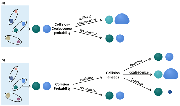
Modelling collisions between droplets in Cleo can be done with or without collisional breakup and rebound. Collisional breakup during rainfall has been observed in situ and has been suggested as an important control on the timing and intensity of rain in LES (Seifert et al., 2005; Testik and Rahman, 2017). Since breakup converts large droplets into significantly smaller ones, its effect on the higher moments of the droplet size distribution can be appreciable (e.g. Hu and Srivastava, 1995; McFarquhar, 2004; Stevens and Seifert, 2008; Straub et al., 2010; Morrison and Milbrandt, 2011; Planche et al., 2019). This motivates two alternative treatments for collisions in Cleo, schematised in Fig. 2, which are:

• a.

  the original algorithm of Shima et al. (2009) which models only collision-coalescence,

• b.

  the extended algorithm which also includes rebound and breakup.

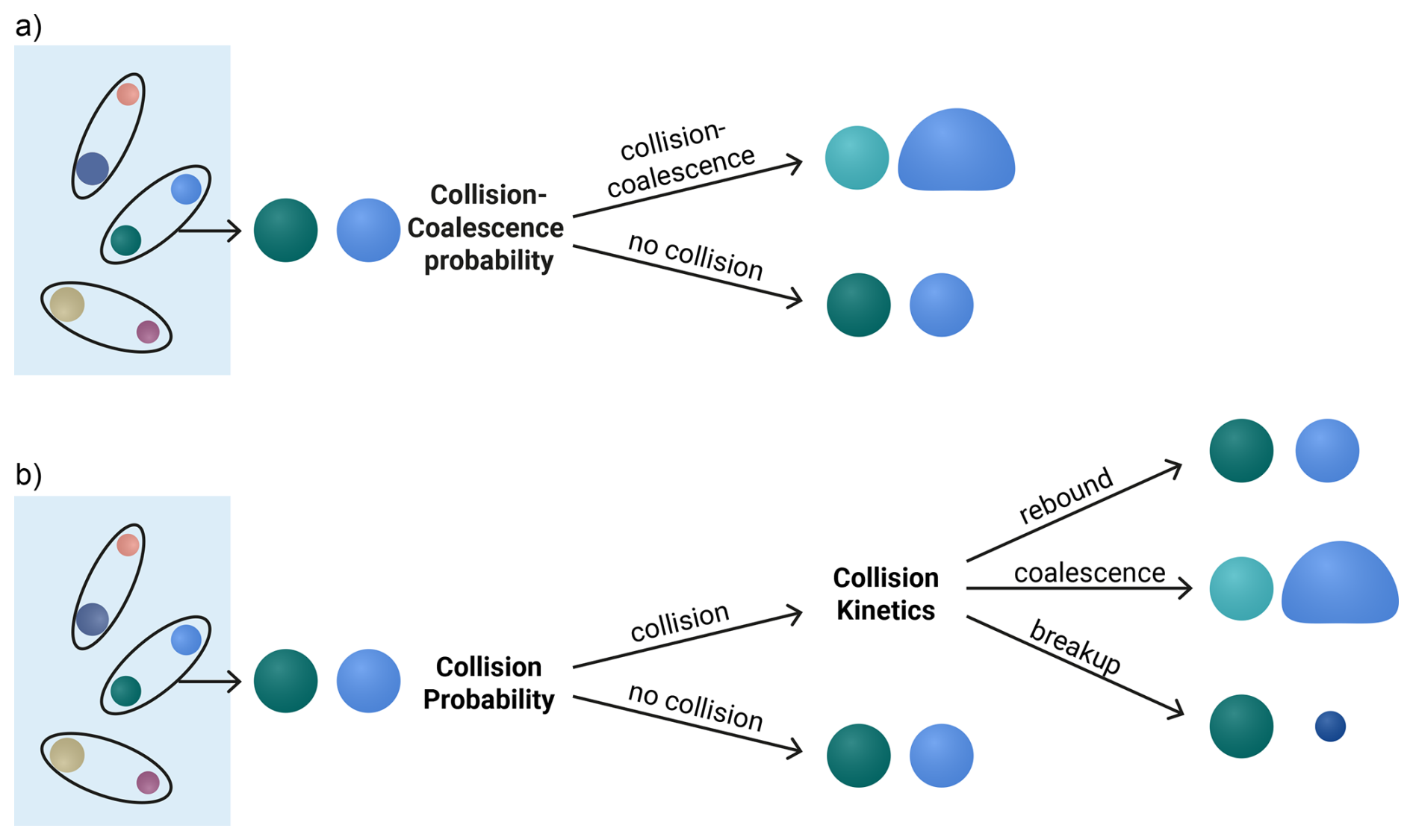
Figure 2 (a) Schematic of the original collision-coalescence algorithm from Shima et al. (2009). (b) The extended collision algorithm including breakup and rebound as well as coalescence. A lightening/darkening of a superdroplet indicates a decrease/increase in its multiplicity.

In both treatments, the steps to determine whether or not a collision occurs is the same as in Shima et al. (2009). All the superdroplets in a grid-box are first randomly paired with one-another. Then for each pair the probability that they collide is compared to a random number, ϕ_α, to determine whether or not a collision is enacted. The probability that two superdroplets collide, p_α, is the probability that two real droplets collide, P_jk, scaled by a factor dependent on the superdroplets' multiplicities. Usually P_jk can be calculated given a collision kernel, K_jk, as

$$\begin{array}{}\text{(8)}& P_{jk}=K_{jk}{\displaystyle \frac{\mathrm{\Delta }{t}_{\mathrm{coll}}}{\mathrm{\Delta }V}},\end{array}$$

for a pair of droplets j and k, where Δt_coll and ΔV are the collision time interval and volume, respectively (Shima et al., 2009). The probability two superdroplets collide is then

$$\begin{array}{}\text{(9)}& p_{\mathit{\alpha }}=max({\mathit{\xi }}_j,{\mathit{\xi }}_k){\displaystyle \frac{n_{\mathrm{s}}(n_{\mathrm{s}}-\mathrm{1})/\mathrm{2}}{\lfloor n_{\mathrm{s}}/\mathrm{2}\rfloor }}{P}_{jk},\end{array}$$

where n_s is the number of superdroplets in the collision volume, ΔV.

Cleo defines the collision probability flexibly to make it easy to switch between different formulations of P_jk. There are large uncertainties in determining the collision probability of a pair of superdroplets' because the collision kernel is so poorly constrained. As such, several formulations for K_jk exist, which differ for example in their treatment of turbulence (e.g. Long, 1974; Hall, 1980; Ayala et al., 2008). The function to calculate P_jk in Cleo can therefore be changed before compilation as long as it still obeys a set of technical constraints on the function's signature (defined by a C++20 concept (ISO, 2020); see also Bayley et al., 2026). There are two P_jk calculations implemented at the time of writing: one for Golovin's kernel (Golovin, 1963), and the other for the hydrodynamic kernel with the formulation for the terminal velocity from Simmel et al. (2002) and collision efficiencies from Long (1974), as also done by Grabowski and Wang (2009). There is no default calculation for the collision probability in Cleo, the user must always specify it during compilation.

If a collision occurs, treatments (a) and (b) differ in their outcome. In the original algorithm, coalescence is assumed and the superdroplets are updated as in Sect. 3.1. In contrast, if a collision occurs in the extended algorithm, the last step of the original collision-coalescence algorithm is modified as shown in Fig. 2b. Rather than assuming a successful collision of two superdroplets results in coalescence, the attributes of the original superdroplets are used to determine if the collision causes rebound, coalescence, or breakup. We then modify the superdroplets to reflect the appropriate outcome: as in Sect. 3.1 for coalescence and as in Sect. 3.2 for breakup. In the event of rebound, the superdroplets remain unchanged.

Cleo has several options for how the attributes of colliding superdroplets determine whether the outcome of the extended algorithm is rebound, coalescence, or breakup. This is physically motivated since properties of droplets, such as their velocities, shapes, and masses, determine whether a collision has sufficient energy to result in coalescence or breakup instead of rebound, but exactly how such properties determine the outcome of a collision is disputed. Our algorithm can therefore easily interchange various formulations from the literature, at the time of writing from Low and List (1982a), Testik (2009) combined with Straub et al. (2010), and Szakáll and Urbich (2018).

As an example, Fig. 3 demonstrates how the outcome of a collision is determined based on Testik (2009) combined with Straub et al. (2010). Let the pair of droplets j and k be re-labelled small, S, and large, L, based on their radii, R_S and R_L respectively. Then, according to Testik (2009), there are three possible regimes depending on the magnitude of the collision kinetic energy, T_E, relative to the surface tension energy of the smaller and larger droplet, S_S and S_L respectively. Using the definitions:

$$\begin{array}{}\text{(10)}& {\displaystyle }& {\displaystyle }{R}_{\mathrm{S}}=\text{min}(R_j,R_k),\text{(11)}& {\displaystyle }& {\displaystyle }{R}_{\mathrm{L}}=\text{max}(R_j,R_k),\text{(12)}& {\displaystyle }& {\displaystyle }{T}_{\mathrm{E}}={\displaystyle \frac{\mathrm{2}}{\mathrm{3}}}\mathit{\pi }{\mathit{\rho }}_{\mathrm{l}}{\displaystyle \frac{R_{\mathrm{S}}^{\mathrm{3}}{R}_{\mathrm{L}}^{\mathrm{3}}}{R_{\mathrm{S}}^{\mathrm{3}}+R_{\mathrm{L}}^{\mathrm{3}}}}|{\mathit{v}}_{\mathrm{S},\mathrm{\infty }}-{\mathit{v}}_{\mathrm{L},\mathrm{\infty }}{|}^{\mathrm{2}},\text{(13)}& {\displaystyle }& {\displaystyle }{S}_i=\mathrm{4}\mathit{\pi }{\mathit{\sigma }}_{\mathrm{l}}{R}_i^{\mathrm{2}}\text{ for }i\in \mathit{\{}\mathrm{S},\mathrm{L}\mathit{\}},\end{array}$$

where ρ_l is the density and σ_l is the surface tension of liquid water, these three regimes are:

1. when T_E<S_S either coalescence or rebound occurs,

2. when $S_{\mathrm{S}}<T_{\mathrm{E}}<S_{\mathrm{L}}$ either coalescence or breakup occurs,

3. when T_E>S_L breakup occurs.

In regimes (1) and (2) a coalescence efficiency, $E_{\mathrm{c}}\in [\mathrm{0},\mathrm{1}]$, is required to give the probability two droplets coalesce, P_c,jk, given that they collided, i.e. $P_{\mathrm{c},jk}=E_{\mathrm{c}}{P}_{jk}$. Here we use the parametrisation for E_c as argued for by Straub et al. (2010), namely that

$$\begin{array}{}\text{(14)}& E_{\mathrm{c}}=e^{-\mathrm{1.15}W},\end{array}$$

where the Weber number, $W=\frac{T_{\mathrm{E}}}{S_{\mathrm{c}}}$, and $S_{\mathrm{c}}=\mathrm{4}\mathit{\pi }{\mathit{\sigma }}_{\mathrm{l}}(R_j^{\mathrm{3}}+R_k^{\mathrm{3}}{)}^{\mathrm{2}/\mathrm{3}}$. In this example and similarly to de Jong et al. (2023a), we draw a new random number ${\mathit{\varphi }}_{\mathit{\alpha }}^{\prime }$ and we compare ${\mathit{\varphi }}_{\mathit{\alpha }}^{\prime }$ with E_c to decide if the collision results in coalescence or the alternative. In general however, the outcome of a collision in Cleo does not need to depend on a second random number, it can instead be calculated from the superdroplet attributes or by rescaling the original random number given the user provides a formula to do so.

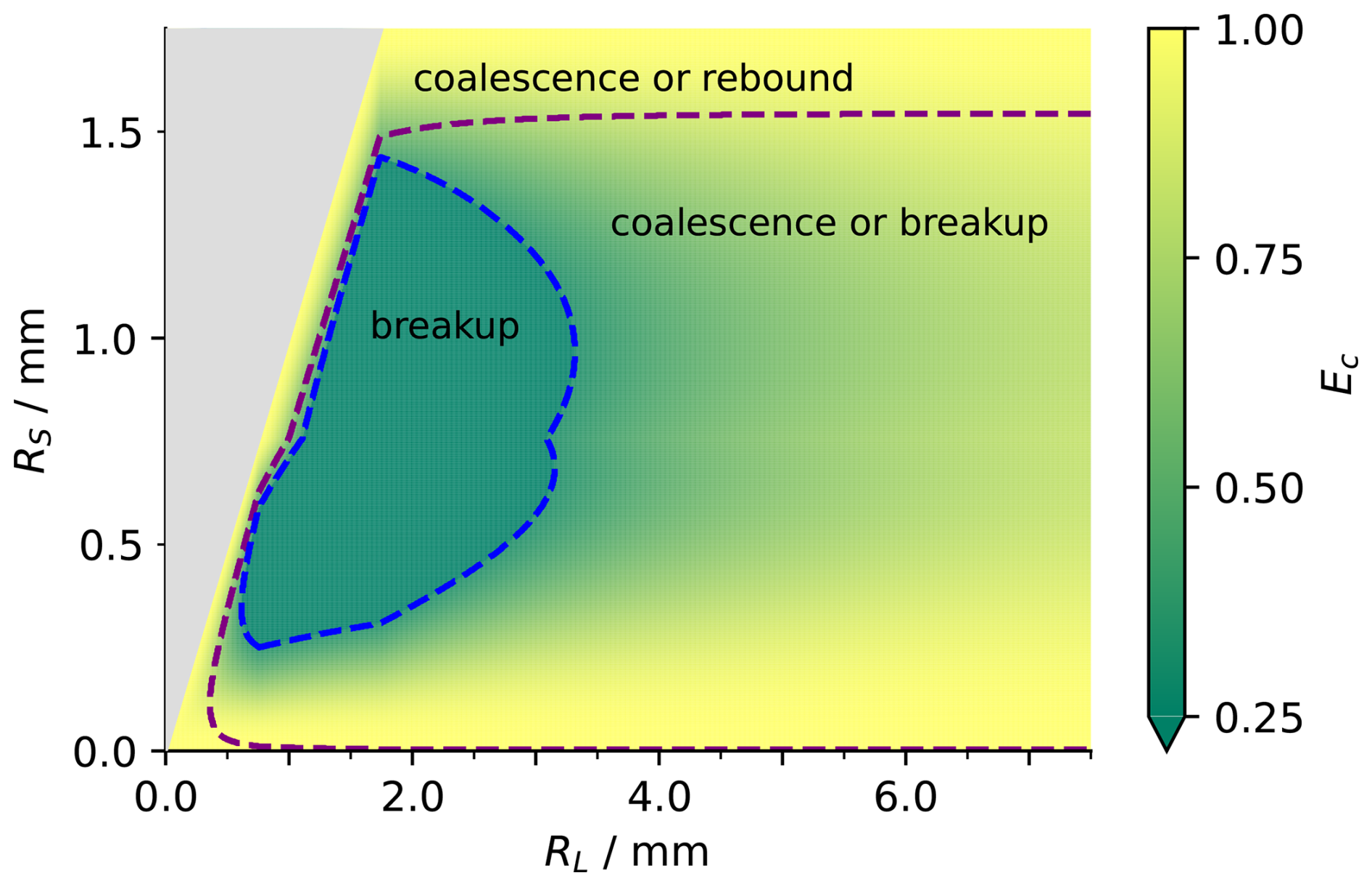
Figure 3 The probability, based on Testik (2009) combined with Straub et al. (2010), for whether a collision between two droplets results in coalescence, rebound or breakup. According to Testik (2009), inside the blue dashed contour it is certain that a collision results in breakup, between the blue and purple contours it may result in coalescence or breakup, and outside the purple contour it may result in coalescence or rebound. The colour gives the coalescence efficiency, in other words the probability of coalescence given that a collision occurs, according to Straub et al. (2010).

3.1 Coalescence

The change in attributes of a pair of superdroplets that undergo coalescence follows Shima et al. (2009) and is illustrated in Fig. 4.

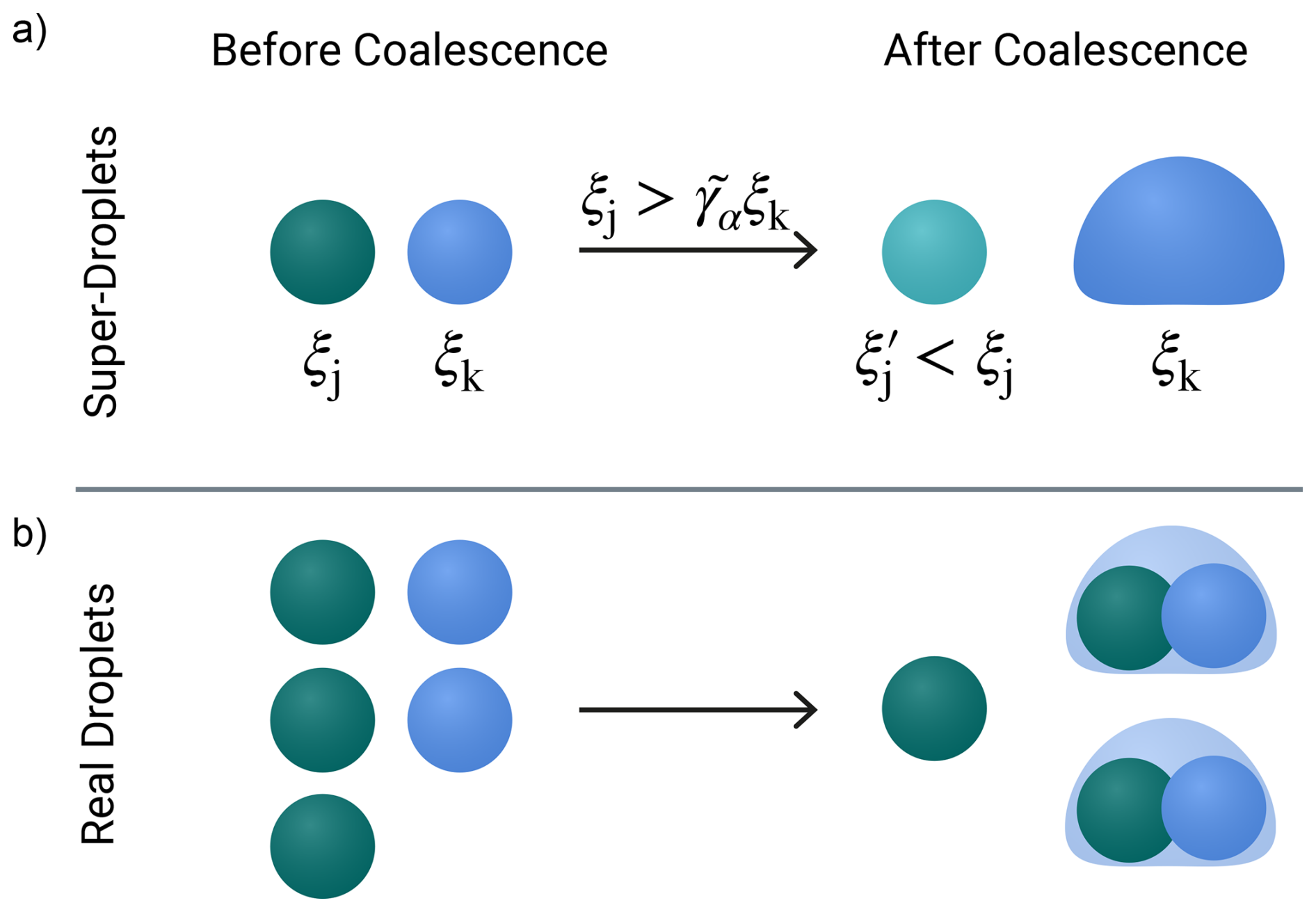
Figure 4 Coalescence as in Shima et al. (2009). (a) The superdroplet representation of coalescence whereby the multiplicity of the more multiplicitous droplet decreases to increase the size of the other superdroplet. A lightening/darkening of a superdroplet indicates a decrease/increase in its multiplicity. (b) The real droplet equivalent of the superdroplets above when ξ_j=3, ξ_k=2 and ${\stackrel{\mathrm{̃}}{\mathit{\gamma }}}_{\mathit{\alpha }}=\mathrm{1}$.

Given a pair of superdroplets (j, k) we can choose without loss of generality the multiplicity of the jth superdroplet to be at least as large as that of the kth, i.e. ξ_j≥ξ_k. The permitted number of consecutive coalescence events, ${\stackrel{\mathrm{̃}}{\mathit{\gamma }}}_{\mathit{\alpha }}$, is then used to determine how the superdroplet attributes are changed to enact coalescence. To calculate ${\stackrel{\mathrm{̃}}{\mathit{\gamma }}}_{\mathit{\alpha }}$, we compare p_α to the random number ϕ_α as well as the multiplicities of the superdroplets since

$$\begin{array}{}\text{(15)}& {\mathit{\gamma }}_{\mathit{\alpha }}=\left\{\begin{array}{ll}\lfloor p_{\mathit{\alpha }}\rfloor +\mathrm{1}& \text{if }{\mathit{\varphi }}_{\mathit{\alpha }}<p_{\mathit{\alpha }}-\lfloor p_{\mathit{\alpha }}\rfloor ,\\ \lfloor p_{\mathit{\alpha }}\rfloor & \text{if }{\mathit{\varphi }}_{\mathit{\alpha }}\ge p_{\mathit{\alpha }}-\lfloor p_{\mathit{\alpha }}\rfloor ;\end{array}\right.\end{array}$$

$$\begin{array}{}\text{(16)}& {\stackrel{\mathrm{̃}}{\mathit{\gamma }}}_{\mathit{\alpha }}=min({\mathit{\gamma }}_{\mathit{\alpha }},\lfloor {\mathit{\xi }}_j/{\mathit{\xi }}_k\rfloor ).\end{array}$$

There are then two possible scenarios which enact coalescence:

• a.

  if ${\mathit{\xi }}_j>{\stackrel{\mathrm{̃}}{\mathit{\gamma }}}_{\mathit{\alpha }}{\mathit{\xi }}_k$, the less multiplicitous superdroplet grows by consuming ${\stackrel{\mathrm{̃}}{\mathit{\gamma }}}_{\mathit{\alpha }}{\mathit{\xi }}_k$ droplets from the other superdroplet,

  $$\begin{array}{}\text{(17)}& {\displaystyle }{\mathit{\xi }}_j^{\prime }={\mathit{\xi }}_j-{\stackrel{\mathrm{̃}}{\mathit{\gamma }}}_{\mathit{\alpha }}{\mathit{\xi }}_k,{\mathit{\xi }}_k^{\prime }={\mathit{\xi }}_k,\text{(18)}& {\displaystyle }{R}_j^{\prime }=R_j,R_k^{\prime }=({\stackrel{\mathrm{̃}}{\mathit{\gamma }}}_{\mathit{\alpha }}{R}_j^{\mathrm{3}}+R_k^{\mathrm{3}}{)}^{\mathrm{1}/\mathrm{3}},\text{(19)}& {\displaystyle }{M}_{\mathrm{s},j}^{\prime }=M_{\mathrm{s},j},M_{\mathrm{s},k}^{\prime }=({\stackrel{\mathrm{̃}}{\mathit{\gamma }}}_{\mathit{\alpha }}{M}_{\mathrm{s},j}+M_{\mathrm{s},k}),\text{(20)}& {\displaystyle }{{\mathit{a}}^{\prime }}_j^{\prime }={{\mathit{a}}^{\prime }}_j,{{\mathit{a}}^{\prime }}_k^{\prime }={{\mathit{a}}^{\prime }}_k;\end{array}$$
• b.

  otherwise ${\mathit{\xi }}_j={\stackrel{\mathrm{̃}}{\mathit{\gamma }}}_{\mathit{\alpha }}{\mathit{\xi }}_k$, and rather than ending up with ${\mathit{\xi }}_j^{\prime }=\mathrm{0}$ both superdroplets are used to represent coalesced droplets,

  $$\begin{array}{}\text{(21)}& {\displaystyle }{\mathit{\xi }}_j^{\prime }=\lfloor {\mathit{\xi }}_k/\mathrm{2}\rfloor ,{\mathit{\xi }}_k^{\prime }={\mathit{\xi }}_k-{\mathit{\xi }}_j^{\prime },\text{(22)}& {\displaystyle }{R}_j^{\prime }=R_k^{\prime }=({\stackrel{\mathrm{̃}}{\mathit{\gamma }}}_{\mathit{\alpha }}{R}_j^{\mathrm{3}}+R_k^{\mathrm{3}}{)}^{\mathrm{1}/\mathrm{3}},\text{(23)}& {\displaystyle }{M}_{\mathrm{s},j}^{\prime }=M_{\mathrm{s},k}^{\prime }=({\stackrel{\mathrm{̃}}{\mathit{\gamma }}}_{\mathit{\alpha }}{M}_{\mathrm{s},j}+M_{\mathrm{s},k}),\text{(24)}& {\displaystyle }{{\mathit{a}}^{\prime }}_j^{\prime }={{\mathit{a}}^{\prime }}_j,{{\mathit{a}}^{\prime }}_k^{\prime }={{\mathit{a}}^{\prime }}_k;\end{array}$$

In the exceptional case that ${\mathit{\xi }}_j^{\prime }=\mathrm{0}$, we currently choose to terminate the simulation rather than remove the superdroplet. We do this because terminating the simulation rather than removing the superdroplet simplifies our algorithms and we do not expect this case to occur in the simulations of mesoscale cloud organisation which Cleo is intended for (which would only contain superdroplets with very large multiplicities). In a future version of Cleo we may amend our algorithms to make Cleo also suitable for simulations of superdroplets with 𝒪(1) multiplicities.

3.2 Breakup

To keep the computational advantages of the original SDM collision algorithm, the fragments created from one breakup event are represented by a single superdroplet. In reality, collisional breakup results in a spectrum of different fragments whose likelihood depends on the two droplets that collided. However the number of simulated particles must be unchanged during collisions to ensure SDM is manageable, and thus the fragments from breakup must all have the same attributes. Ideally these would be randomly sampled from a known fragment distribution, as in de Jong et al. (2023a) and Bringi et al. (2020). However observations of these distributions are limited by both resolution and the undersampling of initial droplet sizes (Low and List, 1982a, b; Schlottke et al., 2010; Prat et al., 2012; Szakáll and Urbich, 2018).

Given the acute shortage of empirical data and our desire for high computational performance, our algorithm does not randomly sample a known fragment distribution. Instead the properties describing the fragments from collisional breakup, ξ_frag, R_frag and M_s,frag, are determined by the initial superdroplet attributes. We provide several ways for how to do this in Cleo; for example, one way asserts mass conservation and that the number of fragments depends on a collision's kinetic energy based on Schlottke et al. (2010), as detailed in Appendix A. Such a method does not seek to reproduce the measured fragment distributions, but rather pursue an overtly simple approach with the intention of exploring whether and how breakup could impact observables such as rain evaporation rates and radar reflectivity signals (e.g. Morrison et al., 2020; Niebaum et al., 2025).

Two previous papers have introduced a collisional breakup algorithm into SDM (Bringi et al., 2020; de Jong et al., 2023a). Unlike the breakup algorithm in McSnow (Bringi et al., 2020), we ensure the conservation of superdroplet number and thus computational tractability. Our algorithm is similar to that of PySDM (de Jong et al., 2023a), but with two adjustments. Firstly, although the step to determine if a collision does or does not occur is always probabilistic (Sect. 3), in general whether a collision then results in rebound, coalescence, or breakup in our algorithm does not have to depend on drawing a new random number, whereas in de Jong et al. (2023a) an additional probabilistic step is always used. Secondly, in the event of breakup we avoid a recursive algorithm by prohibiting multiple breakup events in a single time-step. In the original algorithm of Shima et al. (2009), consecutive coalescence events can be enacted in a single time-step via the factor for the permitted number of consecutive coalescence events, ${\stackrel{\mathrm{̃}}{\mathit{\gamma }}}_{\mathit{\alpha }}$. Allowing consecutive coalescence rests on the assumption that after the first coalescence event(s) the droplets are similar enough that the coalescence probability is approximately unchanged, meaning the collision probability and its outcome do not need recalculation before subsequent events. In our breakup algorithm we make the opposite assumption: that after a single breakup event there is negligible probability of the resultant droplets undergoing further collisional breakup with one-another and thus only one breakup event can occur per time-step (${\stackrel{\mathrm{̃}}{\mathit{\gamma }}}_{\mathit{\alpha }}=\mathrm{1}$). This is a reasonable assumption for the 𝒪(1 s) time-step required for collision-coalescence and is a necessary reduction to the computational cost of the algorithm in large simulations.

The change in superdroplets that undergo collisional breakup is illustrated in Fig. 5 and has two cases analogous to coalescence:

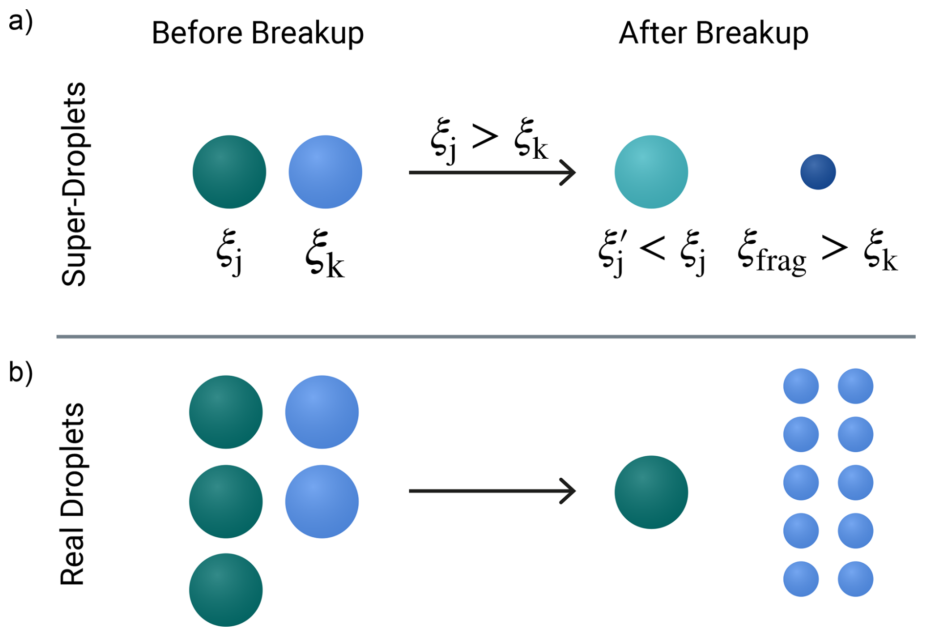
Figure 5 (a) The superdroplet representation of breakup decreases the multiplicity of the more multiplicitous droplet to fragment the other droplet. A lightening/darkening of a superdroplet indicates a decrease/increase in its multiplicity. (b) The real droplet equivalent of the superdroplets above when ξ_j=3, ξ_k=2, and ξ_frag=10.

• a.

  if ξ_j≠ξ_k, we can choose without loss of generality ξ_j>ξ_k such that ξ_k droplets from the more multiplicitous superdroplet are involved in the breakup with the other superdroplet,

  $$\begin{array}{}\text{(25)}& {\displaystyle }{\mathit{\xi }}_j^{\prime }={\mathit{\xi }}_j-{\mathit{\xi }}_k,{\mathit{\xi }}_k^{\prime }={\mathit{\xi }}_{\mathrm{frag}},\text{(26)}& {\displaystyle }{R}_j^{\prime }=R_j,R_k^{\prime }=R_{\mathrm{frag}},\text{(27)}& {\displaystyle }{M}_{\mathrm{s},j}^{\prime }=M_{\mathrm{s},j},M_{\mathrm{s},k}^{\prime }=M_{\mathrm{s},\mathrm{frag}},\text{(28)}& {\displaystyle }{{\mathit{a}}^{\prime }}_j^{\prime }={{\mathit{a}}^{\prime }}_j,{{\mathit{a}}^{\prime }}_k^{\prime }={{\mathit{a}}^{\prime }}_k;\end{array}$$
• b.

  if ξ_j=ξ_k, both superdroplets are used to represent the result of breakup,

  $$\begin{array}{}\text{(29)}& {\displaystyle }{\mathit{\xi }}_j^{\prime }=\text{round(}{\mathit{\xi }}_{\mathrm{frag}}/\mathrm{2}),{\mathit{\xi }}_k^{\prime }={\mathit{\xi }}_k-\text{round(}{\mathit{\xi }}_{\mathrm{frag}}/\mathrm{2}),\text{(30)}& {\displaystyle }{R}_j^{\prime }=R_k^{\prime }=R_{\mathrm{frag}},\text{(31)}& {\displaystyle }{M}_{\mathrm{s},j}^{\prime }=M_{\mathrm{s},k}^{\prime }=M_{\mathrm{s},\mathrm{frag}},\text{(32)}& {\displaystyle }{{\mathit{a}}^{\prime }}_j^{\prime }={{\mathit{a}}^{\prime }}_j,{{\mathit{a}}^{\prime }}_k^{\prime }={{\mathit{a}}^{\prime }}_k;\end{array}$$

3.3 Collisions: Limitations

Cleo also has certain limitations related to its representation of collisions. Our decision to follow the original collision algorithm of Shima et al. (2009) means we are restricted to using a linear sampling for superdroplet pairs (although this is unlikely to be an issue; Dziekan and Pawlowska, 2017), and we do not implement any sub-time-stepping during collisions – for example as done in the latest version of PySDM (de Jong et al., 2023b). Terminating the simulation if superdroplet multiplicities reach zero during coalescence also makes Cleo currently unsuitable for modelling superdroplets with 𝒪(1) multiplicities.

4 Droplet Motion

We use a simple predictor-corrector method to model droplet motion. One of the most computationally expensive parts to Lagrangian microphysics is the motion of particles throughout the domain (Matsushima et al., 2023; Bayley et al., 2026). However, since a superdroplet's location is not the true location of the droplets it represents, there is no imperative to precisely resolve a superdroplet's position. Indeed looking at the conceptual picture of SDM, perhaps the most suitable choice for superdroplet motion would be probabilistic, similar to Curtis et al. (2017). However, we save expense by choosing Heun's method, a second-order predictor-corrector method, with a simple linear interpolation of the wind velocity. This method by construction preserves the divergence of the flow field, and gives physically consistent results at a 1 s time-step (Grabowski et al., 2018).

In summary, we integrate the equation for the coordinates x_i of the ith superdroplet,

$$\begin{array}{}\text{(33)}& {\displaystyle \frac{\mathrm{d}{\mathit{x}}_i\left(t\right)}{\mathrm{d}t}}={\mathit{u}}_i({\mathit{x}}_i,t),\end{array}$$

where the superdroplet's velocity, u_i(x_i,t), is

$$\begin{array}{}\text{(34)}& {\mathit{u}}_i({\mathit{x}}_i,t)=\mathit{w}({\mathit{x}}_i,t)+{\mathit{v}}_{i,\mathrm{\infty }}\left({\mathit{x}}_i\right),\end{array}$$

and ${\mathit{v}}_{i,\mathrm{\infty }}\left({\mathit{x}}_i\right)=-v_{i,\mathrm{\infty }}\left({\mathit{x}}_i\right)\widehat{\mathit{z}}$ is the superdroplet's terminal velocity, and w(x_i,t) is the wind velocity, obtained by simple linear interpolation of the wind velocity at a grid-box's faces. In Cleo the terminal velocity is defined, analogously to the collision probability (Sect. 3), by a set of technical constraints on the signature of the function which calculates it (using a C++20 concept (ISO, 2020); see also Bayley et al., 2026), meaning that different formulations can be easily interchanged. Also analogously to the collision probability, there is also no default calculation for the terminal velocity in Cleo, the user must always specify which one to use during compilation. The options currently available are depicted in Fig. 6. Using the notation ${\mathit{x}}_i\left(t^n\right)={\mathit{x}}_i^n$, and the time-step for superdroplet motion, Δt_m, the predicted coordinates at the subsequent time-step are

$$\begin{array}{}\text{(35)}& {\stackrel{\mathrm{̃}}{\mathit{x}}}_i^{n+\mathrm{1}}={\mathit{x}}_i^n+{\mathit{u}}_i^n\left({\mathit{x}}_i^n\right)\mathrm{\Delta }{t}_{\mathrm{m}},\end{array}$$

which are corrected to

$$\begin{array}{}\text{(36)}& {\mathit{x}}_i^{n+\mathrm{1}}={\mathit{x}}_i^n+\left[{\mathit{u}}_i^n\left({\stackrel{\mathrm{̃}}{\mathit{x}}}_i^{n+\mathrm{1}}\right)+{\mathit{u}}_i^n\left({\mathit{x}}_i^n\right)\right]{\displaystyle \frac{\mathrm{\Delta }{t}_{\mathrm{m}}}{\mathrm{2}}}.\end{array}$$

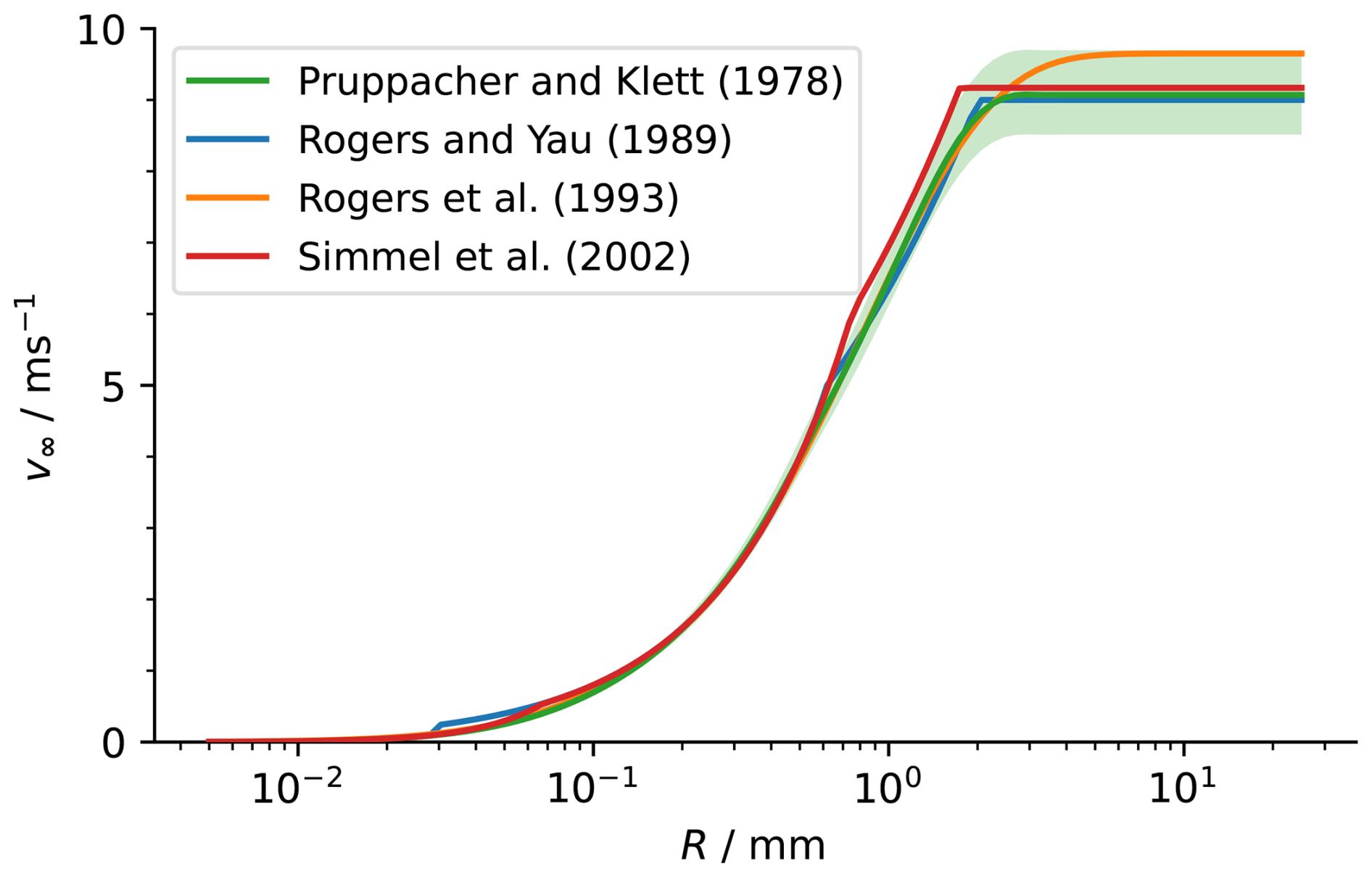
Figure 6 The formulations for terminal velocity currently available in Cleo (Rogers and Yau, 1989; Rogers et al., 1993; Simmel et al., 2002), and for comparison the formulation according to Pruppacher and Klett (1978) at $T=(\mathrm{288.15}\pm \mathrm{15.00})\mathrm{K}$ in a standard atmosphere. In all the formulations, droplets with a radius larger than approximately 3 mm have the same terminal velocity.

This formulation for droplet motion could easily be extended to account for the effects of particle inertia and sub-grid scale turbulence, for example following Naumann and Seifert (2015), which would increase the fidelity of the particle trajectories, especially for large droplets whose inertial relaxation timescale is larger than Kolmogorov time scale.

Droplet Motion: Limitations

As already mentioned, Cleo uses a simple second-order method for droplet motion and does not yet incorporate any stochastic element to represent sub-grid scale turbulent effects on droplet motion. For simulations with increasingly high resolution and low superdroplet multiplicities, it may become more desirable to use a higher order method or one with adaptive sub-time-stepping, as done by some other SDMs (e.g. Naumann and Seifert, 2015; de Jong et al., 2023b), because in such simulations the superdroplet positions more precisely correspond to the real droplets' positions. Especially in coarse resolution simulations, neglecting sub-grid scale turbulence in droplet motion is idealistic, and so in a later version of Cleo our method should be extended to include a stochastic component, e.g. following Dziekan et al. (2019). During superdroplet motion we also make two more minor assumptions, first, we neglect any momentum exchange between the air and droplets (unlike Shima et al., 2020), and second, we assume each particle reaches their terminal velocity instantaneously, since this is unlikely to be noticeable in LES (Naumann and Seifert, 2015). Our method for superdroplet motion is therefore most similar to the other SDMs described by Arabas et al. (2015); Jaruga and Pawlowska (2018), Chandrakar et al. (2021), and Matsushima et al. (2023).

5 Coupling Cleo to a Host Dynamical Driver

Cleo is designed to run SDM microphysics concurrently to any host dynamical driver which it couples to (for the computational implementation see Bayley et al., 2026). For a certain simulation, there are therefore two distinct grids composing the domain at play: Cleo's Eulerian grid and the Eulerian grid of the driver, and these are completely independent except during coupling when information is sent between the two. Cleo's grid can be any kind of Arakawa C-grid and is composed of grid-boxes which define the volumes of the domain and the necessary Eulerian thermodynamic and wind fields so that the Lagrangian superdroplets can enact microphysics and move around. These are: the temperature, pressure, water vapour mass mixing ratio, and liquid water mass mixing ratio defined at the centre of each of Cleo's grid-boxes, as well as the wind velocity defined on the faces of each grid-box. (The meridional wind component is defined at the centre of the faces perpendicular to north-south, and analogously for the zonal and vertical wind components.)

Cleo can be one-way or two-way coupled to a host dynamical driver. In both cases, at the start of each coupling time-step the host dynamical driver, via the coupler, communicates each of the necessary thermodynamic and wind fields to Cleo's grid-boxes. Cleo then enacts SDM microphysics and droplet motion, which potentially alters the temperature, water vapour and liquid water in each grid-box but not the pressure nor winds (e.g. condensation increases temperature and converts water vapour to liquid). In a two-way coupling Cleo then communicates the thermodynamic fields back to host dynamical driver, whereas in a one-way coupling it does not. As long as it can provide the required fields for Cleo, the host dynamical driver can be anything, from analytical formulae, to reading data from files, all the way to a fully-fledged numerical weather or climate model. Any potential advection of thermodynamic fields, momentum feedbacks, radiation or turbulence schemes are the responsibility of the particular host dynamical driver which Cleo is coupled to. For further details of Cleo's time-stepping, coupling or domain composition, readers should refer to Bayley et al. (2026).

6 Model Verifications

This section presents three test-cases which demonstrate the behaviour of our numerical methods for condensation/evaporation, collisions between droplets, and droplet motion individually. Thereafter we present a final integrated test-case applying all three methods at once using the 1-D Kinematic Driver (KiD) modelling framework (Shipway and Hill, 2011, 2012). Additionally, the Supplement to this paper contains two further validations, of droplet collisions and of droplet motion.

6.1 Verification of Condensation/Evaporation

Figure 7 shows the results from Cleo for the same test-case as described in Sect. 7 of Arabas and Shima (2017) for the adiabatic expansion/contraction of a rising/falling volume of air through a hydrostatically equilibrated atmosphere. We used 0.0 and 0.01 for the relative and absolute tolerances of our ODE solver, and 50 and 1 ms for the maximum number of Newton-Raphson iterations and minimum sub-time-step, respectively.

Each column shows the evolution of the air mass given a certain number concentration and/or initial radius of its dry aerosol mono-size distribution. In particular, it shows how the displacement, supersaturation, and droplet radii evolve given three different mean vertical velocities, 〈w〉, for the ascent/descent of the air mass. The first two columns show that, as expected, the faster the vertical velocity, the higher the dis-equilibrium supersaturation during ascent (and the lower the dis-equilibrium supersaturation during descent). By comparing the first two columns, we can also see that increasing the aerosol concentration lowers the dis-equilibrium supersaturation. All these trends in the supersaturation can be explained by faster vertical velocities and/or fewer aerosol causing the rate at which the relative humidity increases with height to be greater than the rate at which the droplets undergo condensation. Conversely, the lower the vertical velocity and higher the droplet number concentration, the closer the air mass to its equilibrium behaviour, where supersaturation does not exceed 0 % and the radii follow the Köhler curve. In the third column however, the Köhler curve is not approached, because the radii and number concentration are low enough that cusp bifurcation occurs and a sudden “jump” in the droplet growth is observed instead. Due to differing numerics and initial thermodynamic conditions compared to Arabas and Shima (2017), the plots are not completely identical (we use 1000 hPa, 298.15 K, and 98.0 %, for pressure, temperature and relative humidity, respectively), but our supersaturations are within 0.1 % of theirs and we also observe cusp bifurcation, albeit at a slightly smaller radius of 0.03 µm. Notwithstanding these differences, we can say that Cleo is able to reproduce the expected evolution of microphysical and thermodynamic conditions for all three mean vertical velocities.

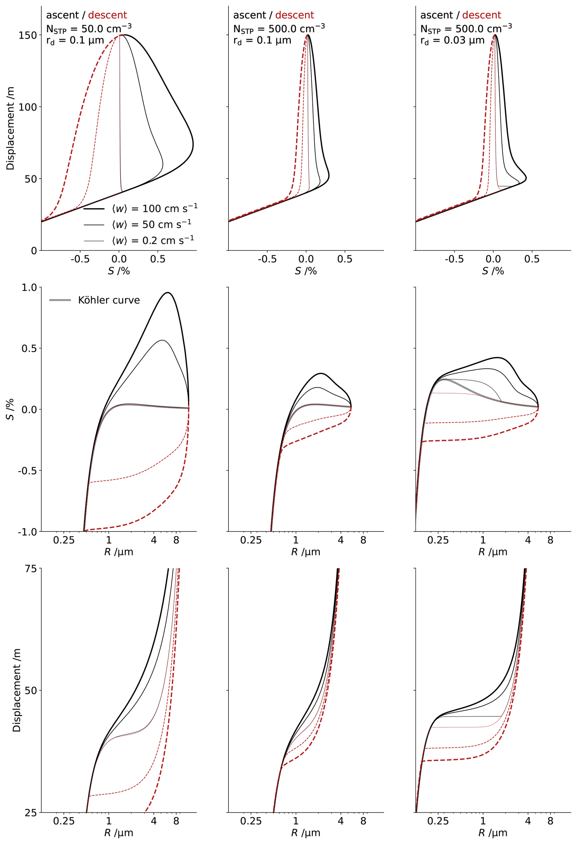
Figure 7 Test of condensation/evaporation as in Arabas and Shima (2017, Sect. 7, Fig. 5). The panels are the same as in Arabas and Shima (2017), except the radius in the third column is 0.02 µm smaller, because slightly different numerics and initial thermodynamic conditions affect the radius at which cusp bifurcation is observed. Each column shows the evolution of an air parcel as it adiabatically rises and falls with a certain number concentration and initial radius of mono-distributed dry aerosol. Top row: the displacement of the parcel against its supersaturation; Middle row: The supersaturation as a function of the droplet radii; Bottom row: the displacement of the parcel against the droplet radii.

To verify qualitatively the effect of ventilation on droplet growth, we ran a second set of adiabatic parcel simulations (Fig. 8). In these simulations we adapted the setup above to demonstrate the behaviour of large droplets falling from a cloud through subsaturated air. We initialised the parcels with wet droplets in 900 hPa pressure, 290 K temperature, and 98.0 % relative humidity, and then let them descend with a constant fall speed until they reached a pressure of 1032 hPa. The wet droplets all had the same dry radius of 0.1 µm but we ran the parcel model with three different initial wet droplet radii: 0.1, 1, and 5 mm, and droplet number concentrations of 0.625, $\mathrm{6.25}\times {\mathrm{10}}^{-\mathrm{3}}$, and $\mathrm{5}\times {\mathrm{10}}^{-\mathrm{6}}$ cm⁻³ respectively, so that the mass of condensed water at the start of each simulation was 2.61 g m⁻³. The fall speed of each parcel was set to approximately the fall speed of the initial droplets, at 1, 5, and 10 m s⁻¹, respectively. For each parcel, we ran the simulation once with the ventilation factor as in Eq. (3) and once without, in which f_v=1.0.

Figure 8 shows how the ventilation factor increases the evaporation of droplets and consequently affects the parcel's relative humidity. For each parcel the droplet radii decreases faster with ventilation accounted for than without. The droplets which are initially 0.1 mm-sized evaporate completely before the end of the simulation, causing substantial moistening of the parcel and the final relative humidity and droplets' size to be the same regardless of whether ventilation was accounted for (Fig. 8a). However, the relative humidity is significantly higher and the droplets are significantly smaller earlier in the simulation (higher in the atmosphere) with ventilation. Compared to the parcels with 0.1 mm-sized droplets, the parcels with larger droplets are substantially drier, reaching 50 %–60 % relative humidity by the end of the simulations compared to 90 %. This is because the larger droplets have a much lower rate of evaporation and much faster fall speed, which results in much less moistening of the parcel. Also because the evaporation rate is so low, the relative humidity of the parcels increases only by up to a few percent when the ventilation effect is accounted for. However, since the rate of evaporation is up to an order of magnitude larger, the final radii of the droplets are 10–100 µm smaller. In more realistic simulations also using Cleo, this effect has been shown to be even larger and have a significant impact on evaporation in the sub-cloud layer beneath shallow cumuli (Niebaum et al., 2025).

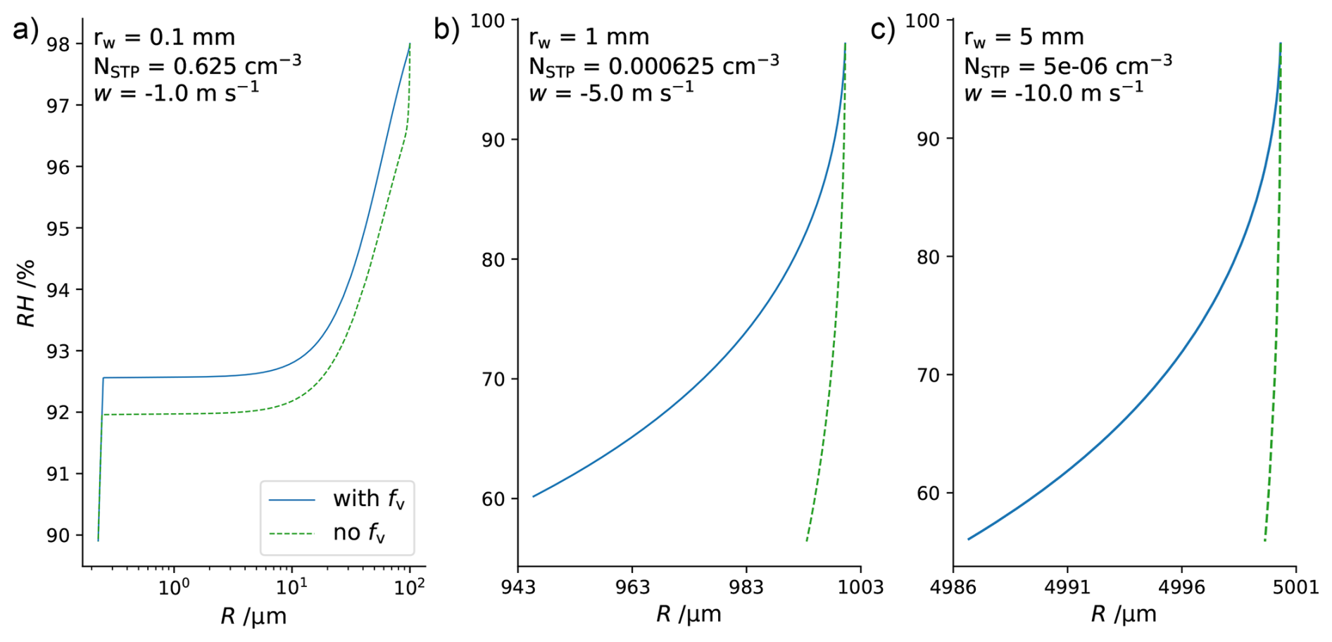
Figure 8 The effect of ventilation on the evolution of wet droplets and relative humidity in falling parcel simulations, for droplets initially with radius, (a) 0.1 mm, (b) 1 mm, and (c) 5 mm. The blue solid lines show simulations accounting for ventilation according to Eq. (3) and the green dashed lines show simulations with f_v=1.0.

6.2 Verification of Collisions

Figure 9 shows the results from Cleo for the same test-case as described in Sect. 5.1.4 of Shima et al. (2009) for the stochastic collisions between water droplets in an arbitrary volume of air. We show results for the same setups as Shima et al. (2009), namely for the evolution of the mass density distribution (normalised by log-space bin-width) given different collision kernels and droplet populations whose volumes are initially exponentially distributed.

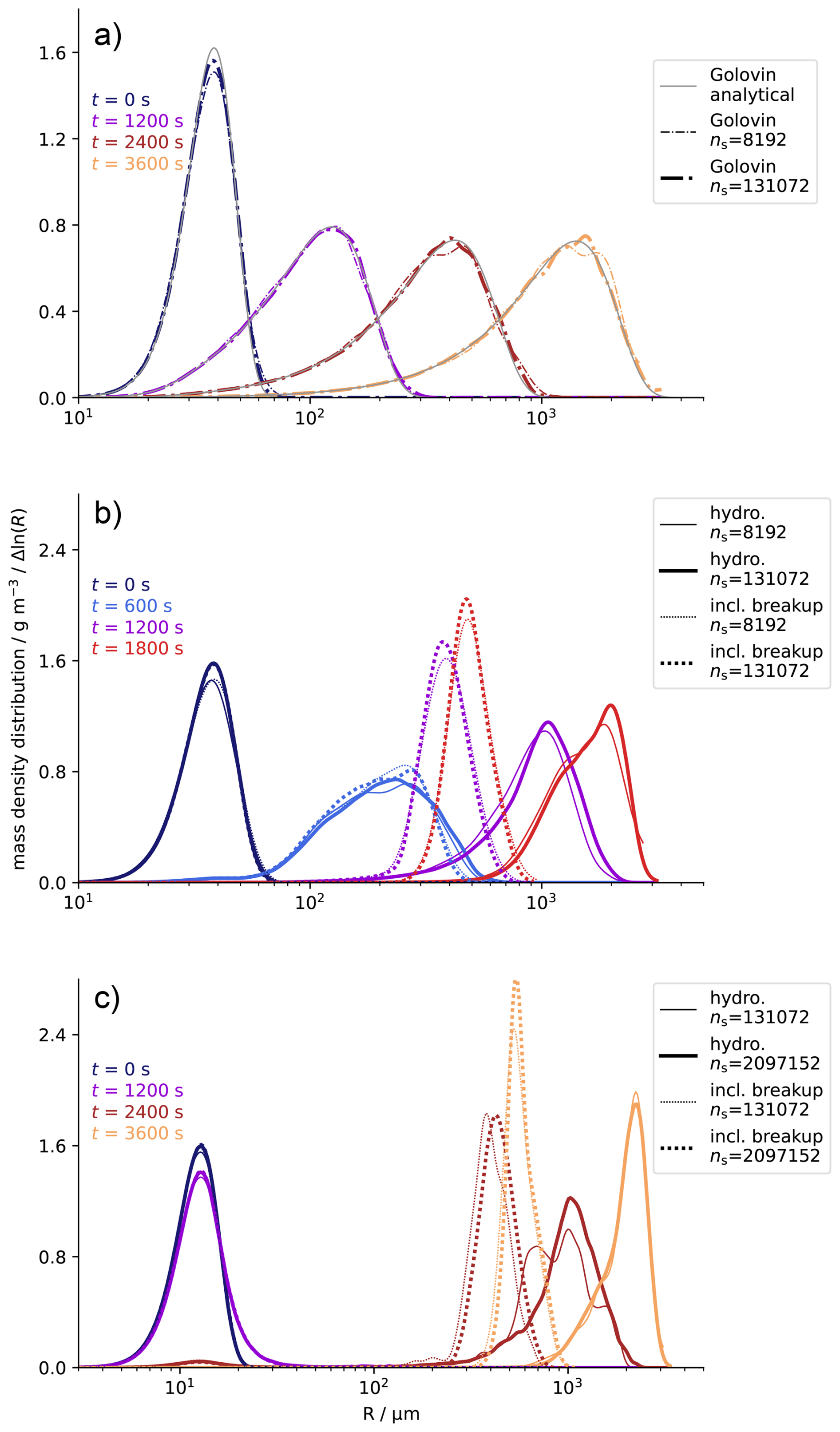
Figure 9 The evolution of the droplet mass density distribution under the tests of the SDM collision algorithm as in Shima et al. (2009, Sect. 5.1.4, Fig. 2). The line-style indicates the collision kernel; the line-width indicates the number of superdroplets, n_s; the colour indicates the time. Panel (a) shows the mass density distribution when using the Golovin kernel for collision-coalescence, as well as its analytical solution (solid grey). Panels (b) and (c) show the tests using the hydrodynamic kernel for collision-coalescence as in Shima et al. (2009), and, additionally, the same tests using the hydrodynamic kernel but when breakup and rebound are also accounted for, using Cleo's extended treatment of collisions with parametrisations based on Testik (2009), Straub et al. (2010), and Schlottke et al. (2010) (see main text, Sect. 3).

Figure 9a shows the evolution when the kernel from Golovin (1963) is used, whereas Fig. 9b–c show the evolution when the hydrodynamic kernel is used. For all cases, we reproduce the results of Shima et al. (2009) when collisions are assumed to result in coalescence. We also demonstrate in Fig. 9b–c how the distribution evolves according to the extended framework from Sect. 3, which also allows for collisional breakup and rebound. The probability of breakup and rebound were calculated from Testik (2009) and Straub et al. (2010) as described in Sect. 3, and if breakup occurred the fragment properties were determined based on the parametrisation of Schlottke et al. (2010) (as described in Appendix A). In Fig. 9b, up to about 600 s the evolution of the droplet size distribution is comparable to the coalescence-only case, but the subsequent growth of droplets is much delayed and converges to a stationary distribution centred at 550 µm, rather than 2400 µm in the coalescence-only case; and qualitatively the same behaviour is seen in Fig. 9c too. As expected, collisional breakup slows and inhibits the growth of mm-size droplets. It also has a much larger impact on the distribution's evolution than changing the collision efficiencies from Long (1974) to Hall (1980) in the coalescence-only case. It remains to be seen how a kernel accounting for turbulent effects would behave, but that too would likely show considerably larger differences (Grabowski and Wang, 2009).

To demonstrate the behaviour of our collisional breakup algorithm in comparison to an approach which uses a parametrised fragment size distribution, we ran a second set of box-model simulations. In these simulations, we compare the stationary droplet size distribution to that reported by Straub et al. (2010, Sect. 5, Fig. 10). This is the same comparison conducted by de Jong et al. (2023a, Sect. 4.1.2, Fig. 9) except that our algorithm does not sample the parametrised fragment size distribution, but rather prescribes a certain number of fragments depending, in general, on the superdroplets which collided (Sect. 3.2). The simulations follow the same setup as Straub et al. (2010), using an initially exponential distribution as expressed by Marshall and Palmer (1948), whereby $p\left(R\right)=N_{\mathrm{mp}}{e}^{-\mathrm{2}{\mathit{\lambda }}_{\mathrm{mp}}R}$ and $N_{\mathrm{mp}}=\mathrm{8}\times {\mathrm{10}}^{\mathrm{6}}{\mathrm{m}}^{-\mathrm{4}}$, ${\mathit{\lambda }}_{\mathrm{mp}}=\mathrm{4.1}\times {\mathrm{10}}^{\mathrm{3}}{R}_{\mathrm{mp}}^{-\mathrm{0.21}}{\mathrm{m}}^{-\mathrm{1}}$, and $R_{\mathrm{mp}}=\mathrm{54}\mathrm{mm}{\mathrm{h}}^{-\mathrm{1}}$. We use 8192 superdroplets to sample the initial droplet size distribution evenly in log-radius-space bins between 0.5 µm and 4 mm (Fig. 10a). To make the results comparable to Straub et al. (2010), in these simulations we do not use the parametrisation from Testik (2009) to include possibility of rebound, but rather we directly determine whether a collision results in either coalescence or breakup by comparing a random number with the Straub et al. (2010) collision efficiency, according to Eq. (14).

Figure 10b shows how the stationary droplet size distribution in Cleo with different parametrisations for the number of fragments compares to the distribution from Straub et al. (2010) with a parametrised fragment size distribution. Using a fixed number of fragments in Cleo, one can sample different parts of the stationary distribution and, as expected, increasing the number of fragments produces a narrower distribution of smaller droplets. Using the parametrisation for the number of fragments given by Schlottke et al. (2010) (as described in Appendix A), the stationary distribution appears qualitatively similar to the cases with a fixed number of fragments, suggesting that the parametrisation tends to produce a similar number of fragments for all collisions which result in breakup in the steady state. In all cases, the shape of the droplet size distribution is narrower than that given by Straub et al. (2010), concentrating more droplets in a smaller size range. A different parametrisation for the number of fragments, for example one which depends on the size of the colliding droplets directly, may show a greater fidelity to the shape of the stationary distribution according to Straub et al. (2010). This example therefore demonstrates how Cleo's overly simple approach to fragment sizes does not seek fully to reproduce measured or parametrised fragment distributions, but rather that the approach can be used to probe upper and lower bounds for the effect breakup could have on a droplet size distribution, for example by using a very high or a very low fixed number of fragments as done by Niebaum et al. (2025).

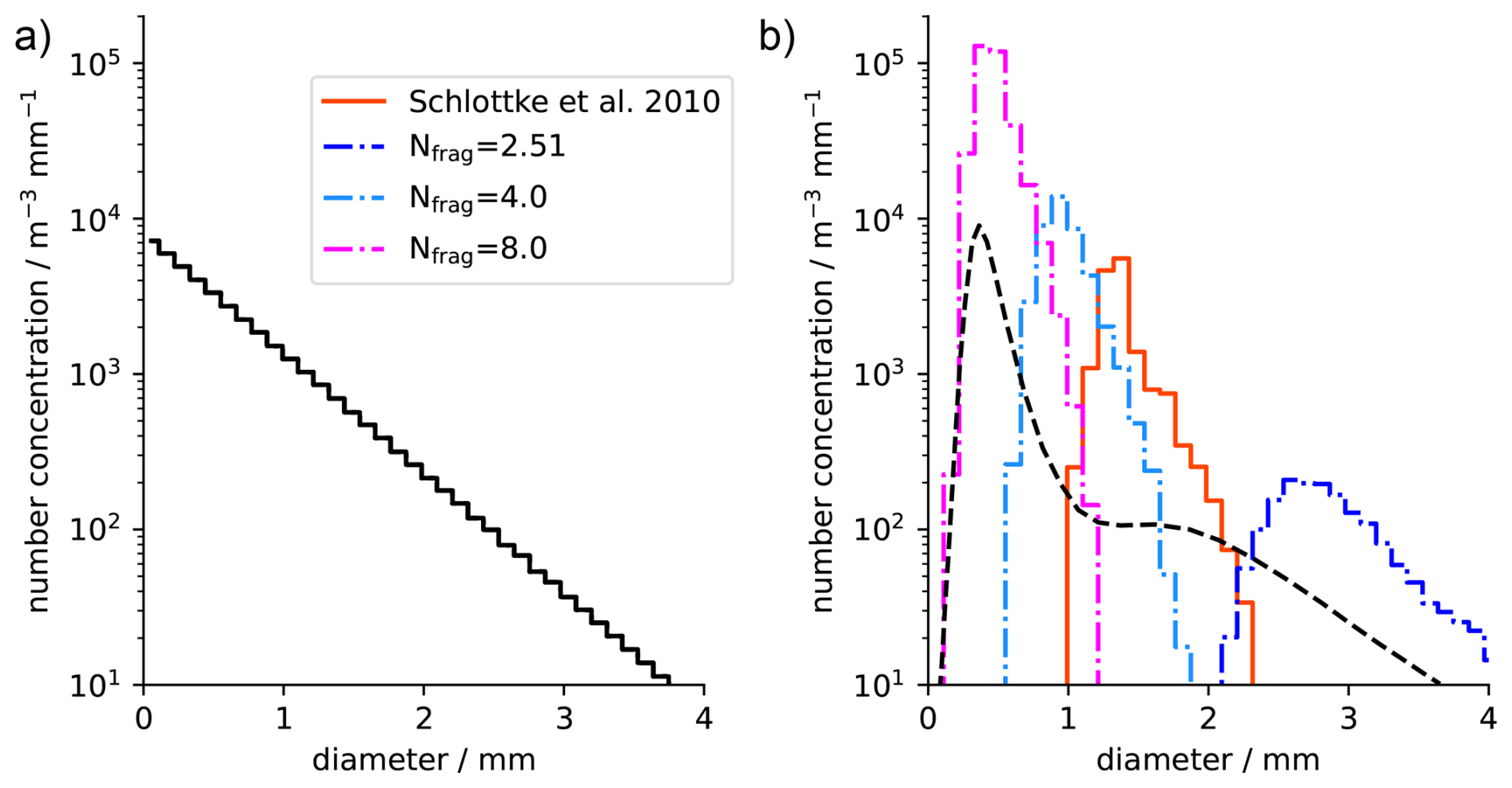
Figure 10 The droplet number concentration distribution normalised by its bin width for (a) the initial droplet size distribution of all the simulations and (b) the stationary droplet size distribution after 7200 s for simulations using Cleo with different parametrisations for calculating the number of fragments in the event of collisional breakup; additionally, a reproduction of the results from Straub et al. (2010) is plotted (black dashed line).

6.3 Verification of Droplet Motion

Figure 11 shows the results from Cleo for the motion of particles in the 2-D kinematic laminar flow model described in Sect. 2.1 of Arabas et al. (2015). 128 superdroplets are initially randomly distributed throughout each grid-box in the domain and the flow is simulated for 1 h with a time-step of 1 s for both motion and data output, and for three simulations with grid-spacing $\mathrm{\Delta }x=\mathrm{\Delta }z=\mathrm{100}$, 50, and 25 m, respectively. We do not simulate microphysics and the droplets have no fall velocity, so the superdroplets behave like tracers for the flow.

As expected, Cleo's particle motion does indeed follow the flow field and respect its divergence-free properties, as confirmed by the conservation of particle number in each grid-box throughout the simulations (Fig. 11d, e, f). Figure 11a, b, c also verifies that increasing the grid resolution increases the accuracy of the particle motion because the interpolation distances in the predictor-corrector algorithm reduce.

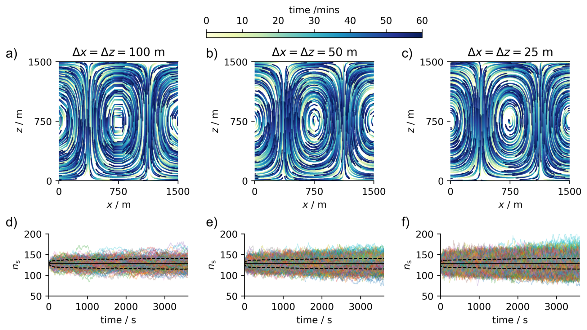
Figure 11 Results of tracer particle motion in the 2-D divergence free laminar flow described by Arabas et al. (2015). Grid-spacing decreases in each column from left to right. Panels (a), (b), and (c) show the trajectories of a random sample of 500 superdroplets; Panels (d), (e), and (f) show the number of superdroplets in each grid-box over time, as well as the mean across all the grid-boxes (black; solid) and the standard deviation (black; dashed). The variance is caused by superdroplets leaving/entering different grid-boxes.

6.4 1-D Kinematic Driver Test-Case

Figure 12 demonstrates the integrated test of Cleo's numerical methods using the 1-D KiD framework. Here we setup the column as described by Shipway and Hill (2012), with a 25 m grid-spacing and sinusoidal updraught velocity for the first 10 min with the maximum speed constant, $w_{\mathrm{1}}=\mathrm{3}\mathrm{m}{\mathrm{s}}^{-\mathrm{1}}$. We couple Cleo via python bindings to PyMPDATA (Bartman et al., 2022a) to advect water vapour, whereas we advect liquid water (superdroplets) within Cleo given the wind field at each time-step (1.25 s). We show results for a 10-member ensemble where for each member we initialise 50 cm⁻³ of dry aerosol throughout the domain by assigning 256 superdroplets per grid-box each a constant multiplicity and randomly sampling a single-mode lognormal distribution with a geometric mean diameter of 0.08 µm and a geometric standard deviation of 1.4, as chosen by Hill et al. (2023). Unlike both Shipway and Hill (2012) and Hill et al. (2023), we specify the initial air density profile to be consistent with hydrostatic equilibrium including the initial water vapour, with the surface pressure at 1000 hPa.

The different microphysics schemes and density profiles causes slight differences between our clouds and those of Shipway and Hill (2012), Hill et al. (2023) and de Jong et al. (2023a), but nevertheless the qualitative behaviour of the test-cases are in agreement and our results lie within the spread amongst different SDMs in Hill et al. (2023). Figure 12a–b shows the liquid water mass mixing ratio, q_l, when only condensation/evaporation is modelled. The cloud reaches a steady state immediately after the updraught velocity terminates, with liquid water content peaking in the middle of our cloud, albeit at a higher value and lower height. Without collision-coalescence, there is no spread across the ensemble members, which indicates little sensitivity of condensation/evaporation to the sampling of the initial dry aerosol distribution, as reported by Hill et al. (2023). In contrast, Fig. 12c–d show the same setup when not only condensation/evaporation, but also collision-coalescence and droplet motion (including their fall velocities) are modelled, and in these simulations the ensemble spread is significant because of the stochasticity in the collision-coalescence algorithm. The mean precipitation onset is around 30 min, in agreement with the range of SDMs in Hill et al. (2023), and likewise the evolution of the liquid water path, cloud droplet number concentration, mean volume diameter and its standard deviation also lie within the SDMs' spread (Fig. 13). More exact agreement is hard to achieve given the ambiguity in the test-case setup and the large model spread reported by Hill et al. (2023), for which further inter-model comparison would be needed to more exactly attribute the discrepancies. Nevertheless, Cleo does indeed behave as expected for a SDM and is in agreement with other microphysics models for warm rain within the KiD framework.

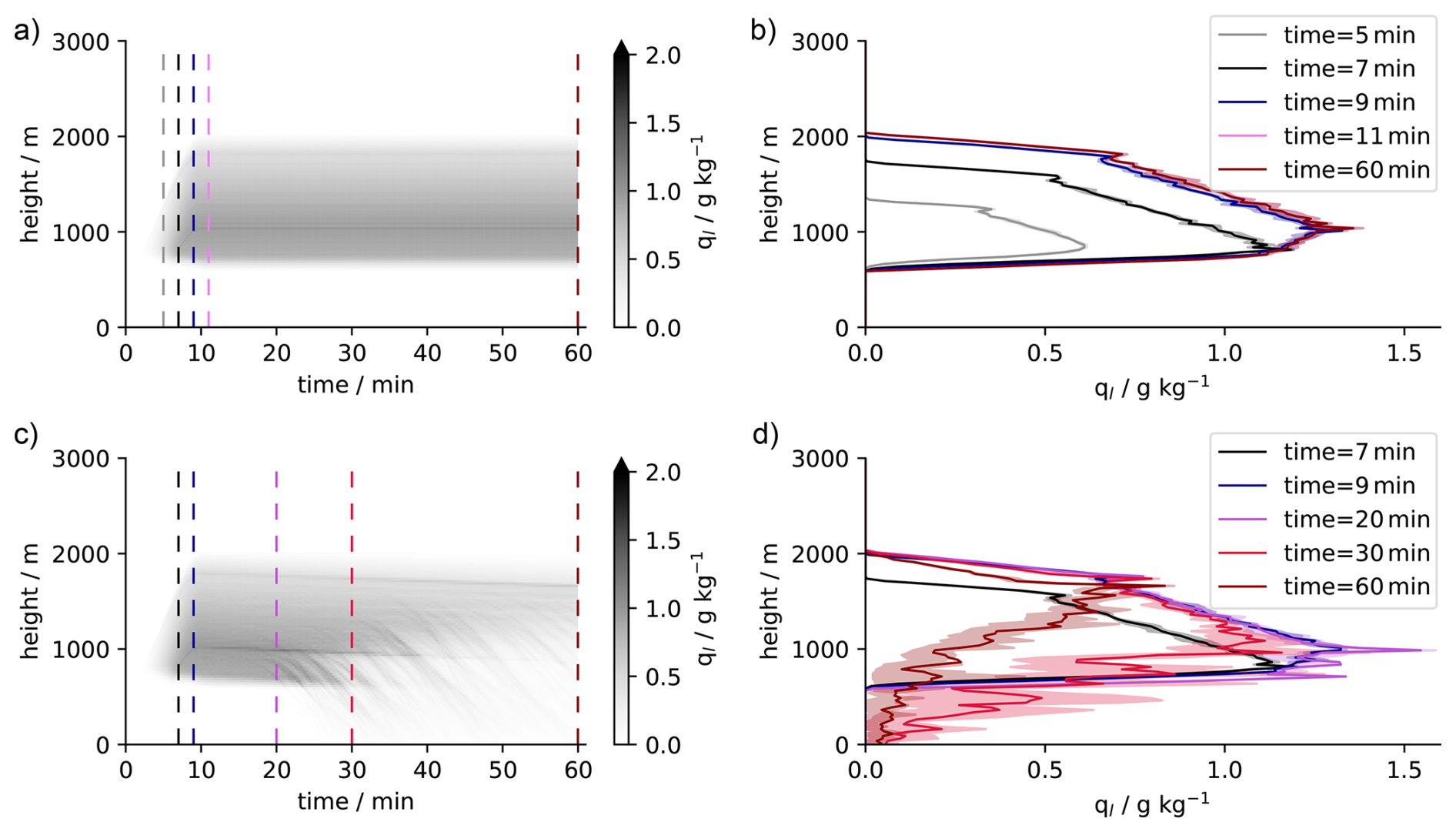
Figure 12 Evolution of the liquid water mass mixing ratio, q_l, during the 1-D KiD test-case: (a–b) only modelling condensation/evaporation, (c–d) modelling condensation/evaporation, collision-coalescence and droplet sedimentation. Results are shown for the mean and interquartile range over an ensemble of 10 members, and figures (b) and (d) are cross sections across the vertical coloured lines in (a) and (b) respectively.

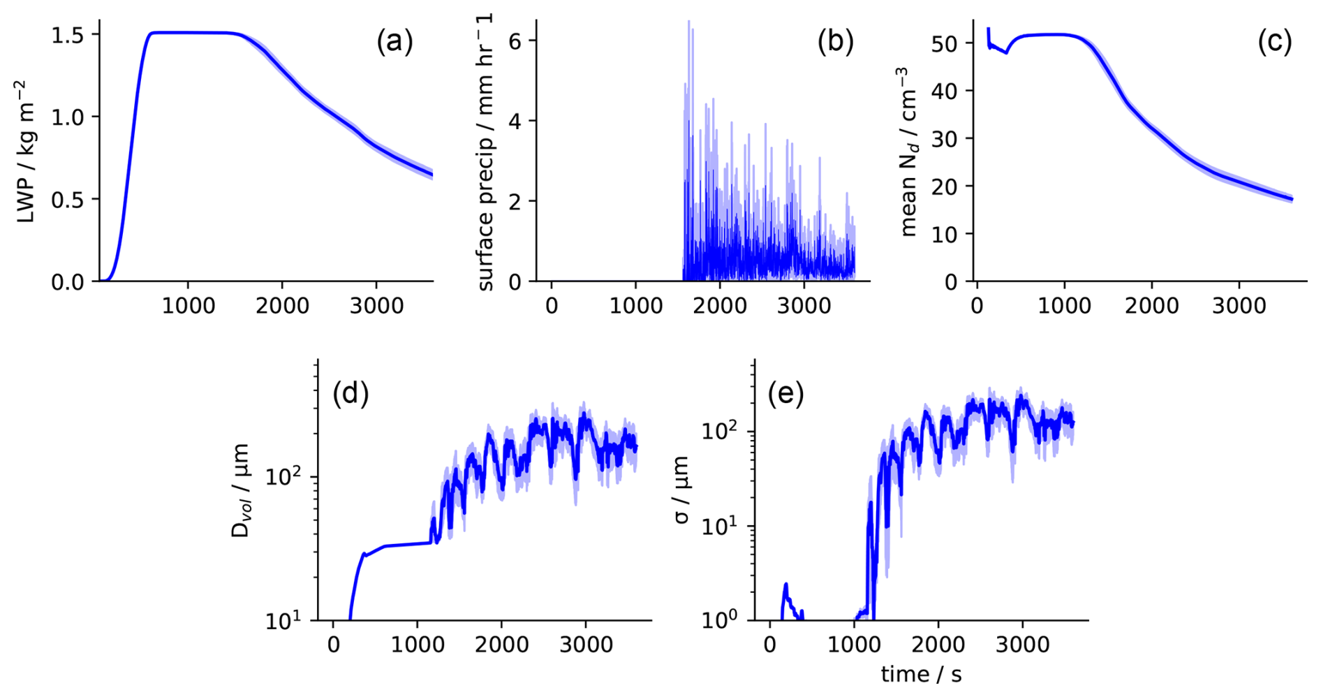
Figure 13 The evolution of (a) the liquid water path, (b) surface precipitation, (c) mean in-cloud droplet number concentration, (d) the mean volume diameter at 700 m, and (e) its standard deviation in our 1-D KiD test-case modelling condensation/evaporation, collision-coalescence and droplet sedimentation. The solid lines are the mean and the shading is the mean ± standard error for the 10-member ensemble. These plots correspond to the plots in Fig. 3a, d, g, j, m (first column) of Hill et al. (2023) but with a smaller ensemble size and without any smoothing they might have used in post-processing.

7 Conclusions

Cleo is a concise and fully-functioning novel implementation of SDM for warm-cloud microphysics. Our primary motivation for creating Cleo is to provide a computationally efficient, “standard” SDM, which we could use in large-enough-domain LES to decipher the interactions between warm-cloud microphysics and shallow mesoscale cloud organisation. Cleo models collisions between droplets and condensation/evaporation, including (de-/re-)activation, similarly to existing SDM implementations albeit with some differences as summarised below. Cleo models Lagrangian particle motion following the SDM of Grabowski et al. (2018) but with the ability to switch between different terminal velocity calculations. In this paper we detailed Cleo's numerical methods for SDM and verified their behaviour against known test-cases for condensation/evaporation, collisions between droplets, and droplet motion, and using an integrated test-case including all three processes in the 1-D KiD framework.

Our numerical methods for condensation/evaporation and collisions between droplets have subtle but noteworthy differences to existing SDM implementations. For condensation/evaporation we solve the Köhler theory ODE explicitly with a number of cost-saving measures including adaptive sub-time-stepping. Our method for condensation/evaporation is thus purposefully very similar to Shima et al. (2009) and Matsushima et al. (2023), except that we additionally incorporate ventilation effects into the ODE we solve. For collisions between droplets, Cleo can use the original collision-coalescence algorithm according to Shima et al. (2009), however Cleo also has various other options, which reflect the uncertainty in the current knowledge about collision probabilities and their outcomes. Therefore Cleo can easily switch between different formulations of the collision kernel and, motivated by a need to investigate the possible influence of collisional breakup on rain evaporation and downdraughts, Cleo includes a framework to model collisional breakup and rebound. We do this in a way that still respects the key features of the original collision-coalescence algorithm by conserving superdroplet number and decreasing the variance in the collisions with decreasing superdroplet multiplicity.

Cleo's numerical methods have some limitations in comparison to some existing SDMs. Regarding condensation/evaporation, perhaps the most significant is that Cleo's method for condensation/evaporation currently does not account for multiple aerosol types. Regarding collisions, we have not incorporated any sub-time-stepping algorithm. Whilst Cleo's simple predictor-corrector method for droplet motion is less expensive than higher-order methods and still preserves the flow-field, is non-diffusive, and has increasing accuracy with increasing grid resolution, it does not yet incorporate turbulent effects and is less precise than a higher order method. All Cleo's limitations and assumptions make it poorly applicable to highly detailed microphysics studies requiring more complex processes, but make it well-designed, as intended, as a simplistic, ordinary representation of warm-cloud microphysics according to SDM.

Not withstanding these limitations Cleo is useful to a broad group of researchers that require a model for warm-cloud microphysics. Simulations can be up to 3-D and can include any combination of the primary microphysical processes behind warm-rain, each with their own independent time-step (and with adaptive time-stepping between different processes, as explained in Bayley et al., 2026). Cleo can be stand-alone, perform “piggybacking” of LES (Grabowski, 2014), or be used as a fully fledged microphysics scheme. Like other SDMs, Cleo provides a precise representation of the droplet size distribution and an intuitive depiction of microphysical processes. We have also made sensitivity studies easy to conduct through Cleo's high-degree of flexibility, whereby microphysics and data output can be easily customised in order to assess the impact of individual microphysical processes (Bayley et al., 2026), potentially for probing microphysical uncertainties and especially those related to droplet collisions. Finally, since Cleo is also well-suited to high-performance computers, it has the potential to be used in more demanding simulations which probe how cloud microphysics and its uncertainties propagate to larger spatial and temporal scales.

Appendix A: Example Parametrisation for Fragments From Collision Breakup

Here we expound one of Cleo's options for how to determine the properties of a superdroplet which represents the fragments from collisional breakup; namely how to define ξ_frag, R_frag and M_s,frag in Sect. 3.2 for Eqs. (25) to (32). As a simple approach for exploring the potential importance of collisional breakup in warm-cloud microphysics, here we assert mass conservation and that the total number of fragments, N_frag, depends on a collision's kinetic energy, T_E. Schlottke et al. (2010) reported that N_frag depends on T_E as:

$$\begin{array}{}\text{(A1)}& N_{\mathrm{frag}}={\left({\displaystyle \frac{\mathrm{3}}{\mathrm{2}}}-(T_{\mathrm{E}}/\mathrm{\mu }\mathrm{J}{)}^{\mathrm{0.135}}\right)}^{-\mathrm{1}}.\end{array}$$

Since this equation diverges at $T_{\mathrm{E}}/\mathrm{\mu }\mathrm{J}={\mathrm{1.5}}^{\frac{\mathrm{1}}{\mathrm{0.135}}}$, we limit N_frag≤25 for $T_{\mathrm{E}}/\mathrm{\mu }\mathrm{J}>\mathrm{16.50}$; and so that collisional breakup always results in more droplets than collided, even when ${\mathit{\xi }}_j={\mathit{\xi }}_k=\mathrm{1}$, we impose the condition that N_frag≥2.5. Both of these amendments are concordant with the experimental data presented by Schlottke et al. (2010).

Given N_frag is the number of fragments produced by a single (real) droplet breakup event, the superdroplet multiplicity must be as follows,

$$\begin{array}{}\text{(A2)}& {\mathit{\xi }}_{\mathrm{frag}}=\text{round(}{\mathit{\xi }}_k\cdot N_{\mathrm{frag}}),\end{array}$$

and therefore, to ensure mass conservation,

$$\begin{array}{}\text{(A3)}& R_{\mathrm{frag}}={\left[{\displaystyle \frac{{\mathit{\xi }}_k}{{\mathit{\xi }}_{\mathrm{frag}}}}(R_j^{\mathrm{3}}+R_k^{\mathrm{3}})\right]}^{\mathrm{1}/\mathrm{3}},\end{array}$$

and

$$\begin{array}{}\text{(A4)}& M_{\mathrm{s},\mathrm{frag}}=\left[{\displaystyle \frac{{\mathit{\xi }}_k}{{\mathit{\xi }}_{\mathrm{frag}}}}(M_{\mathrm{s},j}+M_{\mathrm{s},k})\right].\end{array}$$

Appendix B: Table of Mathematical Notation

(Marshall and Palmer, 1948)(Marshall and Palmer, 1948)(Marshall and Palmer, 1948)

Table B1 Part I of the definitions for all the mathematical notation used in this paper listed in alphabetical order. For brevity “superdroplet” has been abbreviated to “SD” here.

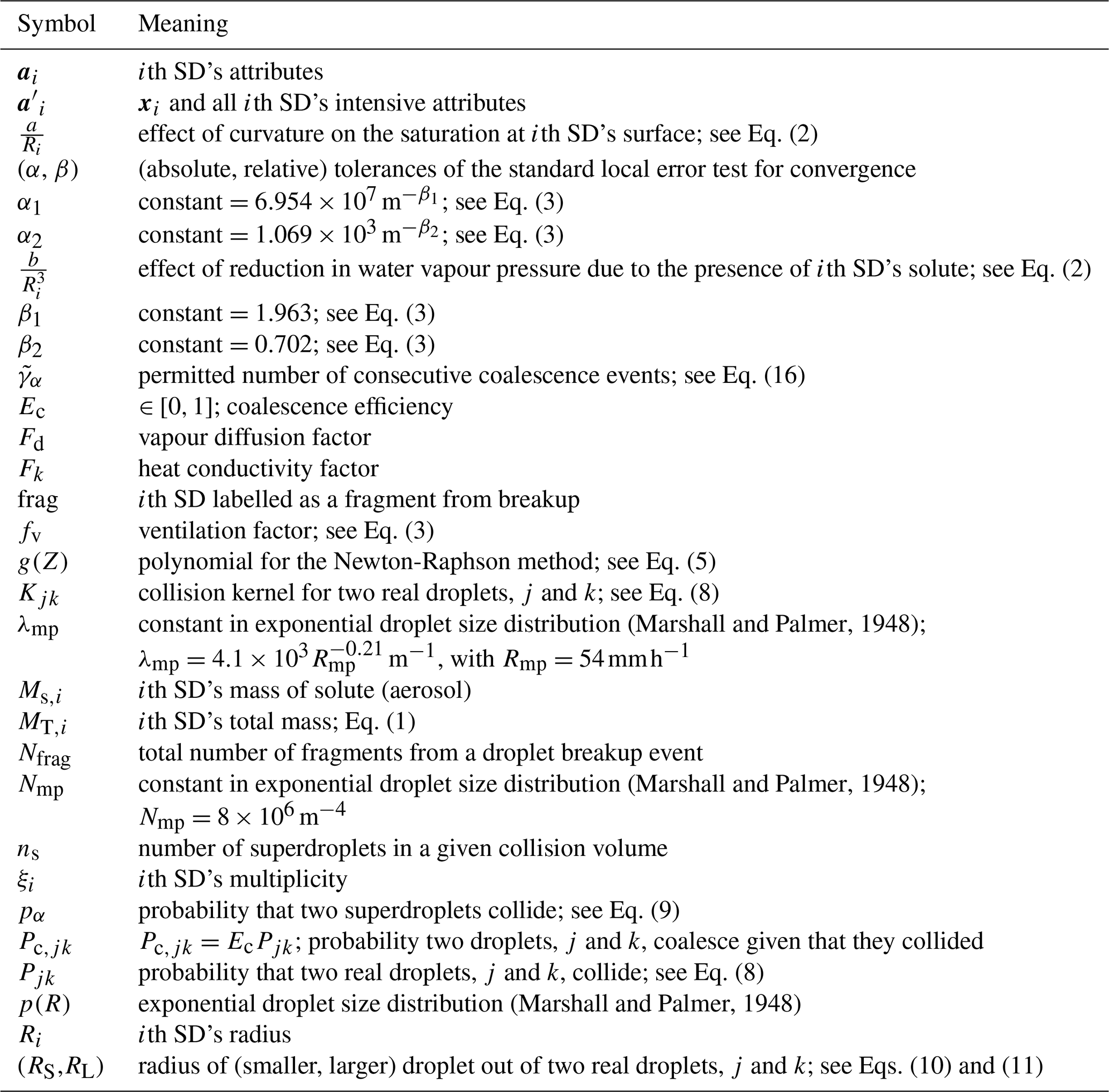
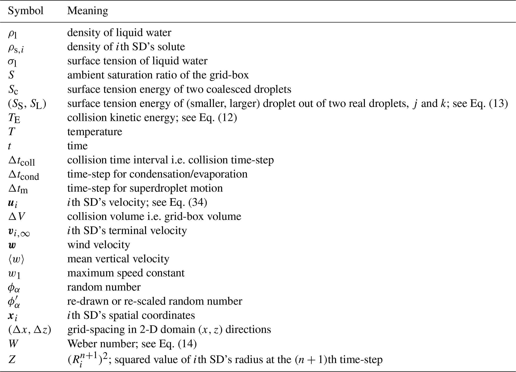
Table B2 Part II of the definitions for all the mathematical notation used in this paper listed in alphabetical order. For brevity “superdroplet” has been abbreviated to “SD” here.