Contribution of physical latent knowledge to the emulation of an atmospheric physics model: a study based on the LMDZ Atmospheric General Circulation Model

In an Atmospheric General Circulation Model (AGCM), the representation of subgrid-scale physical phenomena, also referred to as physical parameterizations, requires computational time which constrains model numerical efficiency. However, the development of emulators based on Machine Learning offers a promising alternative to traditional approaches. We have developed offline emulators of the physics parameterizations of an AGCM, ICOLMDZ, in an idealized aquaplanet configuration. The emulators reproduce the profiles of the tendencies of the state variables for each independent atmospheric column. In particular, we compare Dense Neural Network (DNN) and U-Net models. The U-Net provides better predictions in terms of mean and variance. For the DNN, while it consistently delivers good performances in predicting the mean tendencies, the variability is not well captured, posing challenges for our application. We then investigate why the predictions of the DNN are poorer compared to those of the U-Net, in terms of physical processes. We find that turbulence is not well emulated by the DNN. Leveraging a priori knowledge of how turbulence is parameterized in the phyLMDZ model, we show that incorporating physical knowledge through latent variables as predictors into the learning process leads to a significant improvement of the variability emulated with the DNN model. This improvement brought by the addition of these new predictors is not limited to the DNN, as the U-Net has also shown enhanced results. Preliminary emulations were also performed on a realistic configuration, providing promising results and motivations for further studies. This study hence emphasizes the importance of adding physical knowledge in Neural Network (NN) models to improve predictions and to ensure better interpretability. It opens perspectives on a deeper understanding of the emulator, as well as exploring the contribution of new physical predictors, aiming to make climate simulations and projections.

1 Introduction

Numerical climate models, developed since the 1950s, produce simulations in order to predict the evolution of the state of the atmosphere (Balaji, 2021). These models are used for short-term weather forecasting but are also applied on longer time scales to simulate past and future climates. These models, also known as General Circulation Models (GCM), are crucial for understanding climate mechanisms and projecting future climate change (Manabe and Wetherald, 1975). One of their core components is the atmospheric model, which includes two main distinct components, called the dynamics and physics components. The dynamics component involves solving the Navier-Stokes-like equations on a three-dimensional grid, using a fluid dynamic solver to provide a numerical representation of atmospheric movements (Krasnopolsky et al., 2013). The physics component, which gathers the ensemble of physical parameterizations, is used to represent small-scale phenomena that affect atmospheric dynamics but cannot be explicitly resolved by the dynamical core because its grid is too coarse or because of dynamical assumptions such as the hydrostatic approximation (Balaji et al., 2022). Radiation, orographic waves, exchanges of energy and quantities of matter between the surface and the atmosphere, or cloud formation with vertical atmospheric movements known as convection and cloud-radiation interactions are examples of parameterized subgrid phenomena (Balaji et al., 2022). The dynamical core relies on well-established equations, whereas the parameterizations are based on heuristic/phenomenological/empirical approaches (Hourdin et al., 2017). Specifically, parameterizations are designed to represent the aforementioned phenomena, so that the general behaviour of the atmosphere is reproduced at scales larger than the spatial resolution. The main purpose of a GCM is to iteratively calculate the evolution of state variables that control and describe meteorology and climate, starting from an initial condition and by updating the state of the climate system at each time step. This enables better understanding of past climates, analyses of the current climate and projections for the future climate by modifying boundary conditions and forcings, particularly in terms of greenhouse gas concentration. However, to generate these projections, a large number of simulations have to be carried out to cover the wide range of possible outcomes, sampling the variability of the factors influencing the climate system, including natural processes and human activities. A substantial number of simulations must also be computed due to the non-stationarity of the climate system, which needs to be considered when studying paleoclimates and extreme events. This large number of simulations requires a large computing time, in particular the physical component, which limits the numerical efficiency of the models. Moreover, as approximations, parameterizations of subgrid phenomena are still the source of large uncertainties in climate simulations (Sanderson et al., 2008; Balaji et al., 2022). Progress can be made in the representation of these sub-mesh phenomena, notably by developing a new generation of higher-resolution models (Bauer et al., 2021) or by using Machine Learning (ML) techniques (Schneider et al., 2017).

The burgeoning field of ML techniques opens new horizons, particularly with Deep Learning (DL) and its backbone, Neural Networks (NNs) (LeCun et al., 2015), not only to develop new parameterizations but also to produce accurate, robust and fast emulators of parts of a climate model. In particular, if they reliably reproduce physical processes, they would provide an efficient alternative to traditional process representation. These emulators could then replace one or more parameterizations that are computationally expensive and so, have the potential to enhance numerical efficiency, enabling the exploration of phenomena that are computationally expensive. There is currently a rich literature on the development of physical surrogate models since it is a research topic currently under active development. To provide a context for our study, we will emphasize four key aspects of the emulation of physical processes: the diversity of emulated parameterizations, the model configurations used, the ML algorithms developed and the addition of physical knowledge in the emulator.

Many studies focused on emulating specific existing parameterizations, usually the most expensive ones. These ML algorithms have been developed for ocean parameterizations (Guillaumin and Zanna, 2021) but also for atmospheric parameterizations, such as radiative transfer (Krasnopolsky et al., 2005; Pal et al., 2019; Roh and Song, 2020; Lagerquist et al., 2021; Belochitski and Krasnopolsky, 2021; Meyer et al., 2022), moist convection (Brenowitz and Bretherton, 2018; O'Gorman and Dwyer, 2018; Brenowitz et al., 2020), microphysics (Seifert and Rasp, 2020; Gettelman et al., 2021; Arnold et al., 2023), or even gravity wave drag (Chantry et al., 2021; Espinosa et al., 2022). On the other hand, some studies decided to tackle the emulation of all the parameterizations at once. It is the case of Gentine et al. (2018) and Rasp et al. (2018) who were the first to develop an emulator that learns physics tendencies of embedded Cloud-Resolving Models (CRMs). Their pioneering studies have shown promising results, as they developed an emulator based on Dense Neural Networks (DNNs), using an aquaplanet setup, with good capability to represent convection.

Like Gentine et al. (2018) and Rasp et al. (2018), some studies have opted to simplify the experiment of their model by using idealized aquaplanet configurations (Brenowitz and Bretherton, 2019; Chantry et al., 2021; Beucler et al., 2020; Yuval and O'Gorman, 2021; Behrens et al., 2022), while others have added orography or even continental surfaces directly (Han et al., 2020; Mooers et al., 2021; Wang et al., 2022; Bretherton et al., 2022; Han et al., 2023; Watt-Meyer et al., 2024; Hu et al., 2025), thereby increasing the complexity of the physical processes and making the emulation problem even more challenging.

Another aspect that distinguishes the various studies carried out is the choice of architecture, as a wide range of emulators have been developed using diverse ML designs. ML has been experiencing explosive growth in recent years, leading to increasingly sophisticated algorithms. Initially, DNNs of fully connected layers (Rasp et al., 2018; Pal et al., 2019) were used for emulation tasks, as well as other ML algorithms such as Random Forests (RFs) (O'Gorman and Dwyer, 2018; Limon and Jablonowski, 2023). Yuval et al. (2021) developed an emulator based on a DNN that learns from a high-resolution three-dimensional aquaplanet simulation, specifically capturing unresolved vertical processes that influence thermodynamic and moisture variables. They focused on comparing convection predictions made by the DNN and a RF developed by Yuval and O’Gorman (2020), for the same problem. The offline evaluation – where the emulator is not coupled to the rest of the model – demonstrated that DNN outperformed the RF algorithm while also using less memory. However the two models are comparable when the evaluation is done online. Furthermore, Convolutional Neural Networks (CNN) were introduced for emulation because of their ability to capture spatial and temporal relationships in data (Bolton and Zanna, 2019; Liu et al., 2020). Han et al. (2020) conducted a study to emulate convection and cloud parameterizations in a realistic configuration where the emulator was built from convolutional layers to which residual functions were added, forming a Residual Network (ResNet). In this architecture, the traditional connected layers were replaced by convolution layers. This study achieved good results in predicting temperature and moisture tendencies driven by moist physics processes. This ResNet model proved to be more accurate than a fully connected NN or a conventional CNN. More recently, studies focusing on emulating with advanced architectures have emerged such as U-Nets (Lagerquist et al., 2021; Hu et al., 2025), which have proved effective in handling more intricate multi-scale tasks by capturing spatial features at various resolutions. The results obtained by Heuer et al. (2024) suggest that the U-Net architecture seems to perform better and has a lower error than the other models tested to emulate the convective subgrid fluxes.

In general, emulators can be seen as black boxes due to their lack of interpretability (Reichstein et al., 2019). Incorporating physics-based knowledge into the emulator, either as input or in the architecture itself, can help to improve emulator performance while reducing its black-box character. Some papers have explored techniques to add constraints to the emulator. For instance, Beucler et al. (2019) and Beucler et al. (2021) have incorporated physical knowledge into the loss function and have designed the architecture with conservation layers so that established conservation laws (mass, momentum and energy) are respected when emulating convective processes.

The present work investigates the potential of developing an emulator of the physical parameterizations of the ICOLMDZ Atmospheric General Circulation Model (AGCM) developed at IPSL (Hourdin et al., 2020; Dubos et al., 2015). The emulator could improve numerical performance, as currently almost half of the total computing time is given to the physical part of the model. We will evaluate the capabilities of several emulators aiming to reproduce all the physics of our standard model phyLMDZ while trying to explain their differences in performance. These emulators are based on DNNs and U-Nets. We chose to use DNNs after noticing that even relatively simple fully connected networks yielded promising results as reported in the literature. We also explored more complex architectures, particularly focusing on U-Nets which demonstrate robustness in capturing spatial variations thanks to their encoder-decoder design. In addition, Residual Blocks (ResBlocks) – skipping connections between block input and output to directly learn residual functions – are added to U-Net to facilitate model convergence. Using these models, our focus will be on how integrating physical information into the emulation process can contribute to building more efficient emulators. This work is first conducted using an idealized aquaplanet configuration before proceeding with tests on a more realistic configuration. All emulators are tested in an offline setup without coupling to the dynamics component.

The present paper is structured as follows. Section 2 describes the data used from the ICOLMDZ model, as well as the inputs and outputs of the emulators and the necessary preprocessing steps applied to it. Section 3 is dedicated to the methods used, including a description of the various NN architectures and the evaluation metrics. Section 4 provides an evaluation and a comparison of the first emulators of the physical parameterizations developed for the aquaplanet configuration. Section 5 addresses the motivation for adding physical knowledge and focuses on the evaluation of new emulators that incorporate this physical knowledge as input. Section 6 presents the results on a realistic configuration. In Sect. 7, the results are summarized and discussed, and finally an outline of future work is given.

2 Data

2.1 ICOLMDZ simulation data

We use the IPSL climate model and more particularly its ICOLMDZ atmospheric component (see Fig. 1), which combines two main distinct components: DYNAMICO, the icosahedral dynamical core which solves the equations governing the atmospheric circulation (Dubos et al., 2015), and phyLMDZ, the atmospheric physics component which represents the other processes affecting the atmosphere (Hourdin et al., 2020). We use DYNAMICO at low resolution (200 km). It is composed of an unstructured grid of 16 002 cells and has a vertical resolution of 79 levels. It has the advantage of circumventing the polar singularity, unlike a regular longitude-latitude mesh, thus improving scalability. Like the dynamics part, phyLMDZ runs at a vertical resolution of 79 levels. However, in DYNAMICO, the calculations are performed on the three-dimensional grid, allowing horizontal exchanges with the surrounding grid points whereas phyLMDZ follows a single-column approach. In other words, in phyLMDZ, calculations are done column by column without interaction between them, because subgrid processes involve transport in the vertical direction only.

Figure 1 Scheme of the ICOLMDZ atmospheric model.

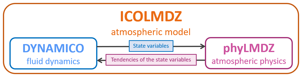
In ICOLMDZ, DYNAMICO provides the state variables, such as temperature, humidity and winds, to phyLMDZ, which then calculates the tendencies associated with each state variable, for each physical phenomenon – or parameterization. We can define a tendency of a variable as the difference between two successive values of a given variable per unit time. For a state variable X at a time t, the total physical tendency ${\left(\frac{\partial \mathit{\text{X}}}{\partial t}\right)}_{\text{phy}}$ resulting from subgrid processes is the sum of the tendencies due to each individual process p, such as:

$$\begin{array}{}\text{(1)}& {\left({\displaystyle \frac{\partial \mathit{\text{X}}}{\partial t}}\right)}_{\text{phy}}=\sum _p{\left({\displaystyle \frac{\partial \mathit{\text{X}}}{\partial t}}\right)}_p\end{array}$$

where p corresponds to the parameterizations. Then, phyLMDZ returns this tendency to DYNAMICO, which calculates the dynamical tendency ${\left(\frac{\partial \mathit{\text{X}}}{\partial t}\right)}_{\text{dyn}}$.

First, we decided to use ICOLMDZ in an idealized aquaplanet setup where the Sea Surface Temperature (SST) is prescribed and depends only on latitude (Medeiros et al., 2016). In this configuration, the diurnal cycle is activated, but the seasonal cycle is not, and there is no topography or continent. Second, we used ICOLMDZ in an Atmosphere Modelling Intercomparison Project (AMIP) experiment (Gates et al., 1999) that provides a more realistic experiment than an aquaplanet since continents, topography and sea ice area are included. SST and Sea Ice Concentration (SIC) are prescribed based on observations (Eyring et al., 2016). Furthermore, the diurnal and seasonal cycles are represented. For both experiments, we did not include the coupling with the land surface component of the IPSL model, ORCHIDEE (Krinner et al., 2005). For each experiment, we ran a one-year long simulation with variables output every 15 min, resulting in 96 time steps per day. This amounts to a total of 34 560 time steps for the entire year. From this simulation, we extracted the boundary conditions, the prognostic state variables and their tendencies. In the following sections of this study, the notation d_X will be adopted to denote the physical tendency of the variable X.

2.2 Input and output variables of emulators

Our goal is to develop a neural network to emulate all the physics of the phyLMDZ model. The input and output variables of the emulator were selected according to the design of the phyLMDZ model and are generated through the ICOLMDZ simulation. The input variables are key quantities computed by the dynamical core and provided to the phyLMDZ model, and also boundary conditions, while the output variables represent the 3D subgrid physics tendencies calculated by phyLMDZ based on these input variables. Diagnostic variables such as precipitation are not considered in our emulation problem.

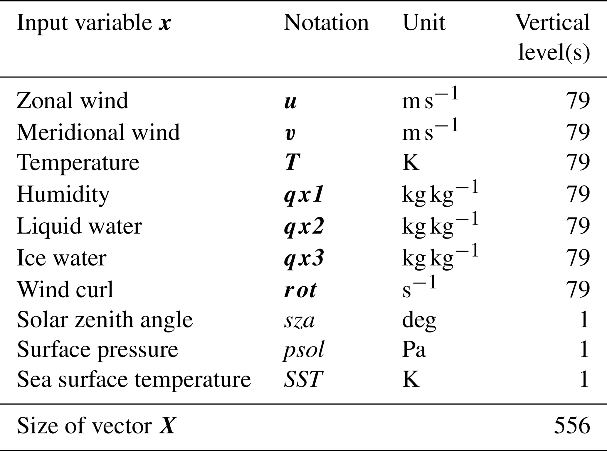
More precisely, the inputs – or predictors – of the neural networks include the vertical profiles of the six state variables with a length of 79, corresponding to vertical levels z, where $z\in \mathit{\{}\mathrm{1},\mathrm{\dots },\mathrm{79}\mathit{\}}$, such as profiles of the zonal wind u, the meridional wind v, the temperature T, the humidity qx1, the liquid water qx2 and the ice water qx3. We also added four other variables: the vertical profile of the wind curl rot used for non-orographic gravity wave drag, and three scalars corresponding to boundary conditions, which are the solar zenith angle sza, the surface pressure psol and the sea surface temperature SST. All of these inputs, listed in Table 1, are concatenated in a vector X of size 556, such as:

$$\mathit{X}=\left[\mathit{u},\mathit{v},\mathit{T},\mathit{q}\mathit{x}\mathit{1},\mathit{q}\mathit{x}\mathit{2},\mathit{q}\mathit{x}\mathit{3},\mathit{r}\mathit{o}\mathit{t},\mathit{\text{sza}},\mathit{\text{psol}},\mathit{\text{SST}}\right].$$

Table 1 List of input variables x for NNs.

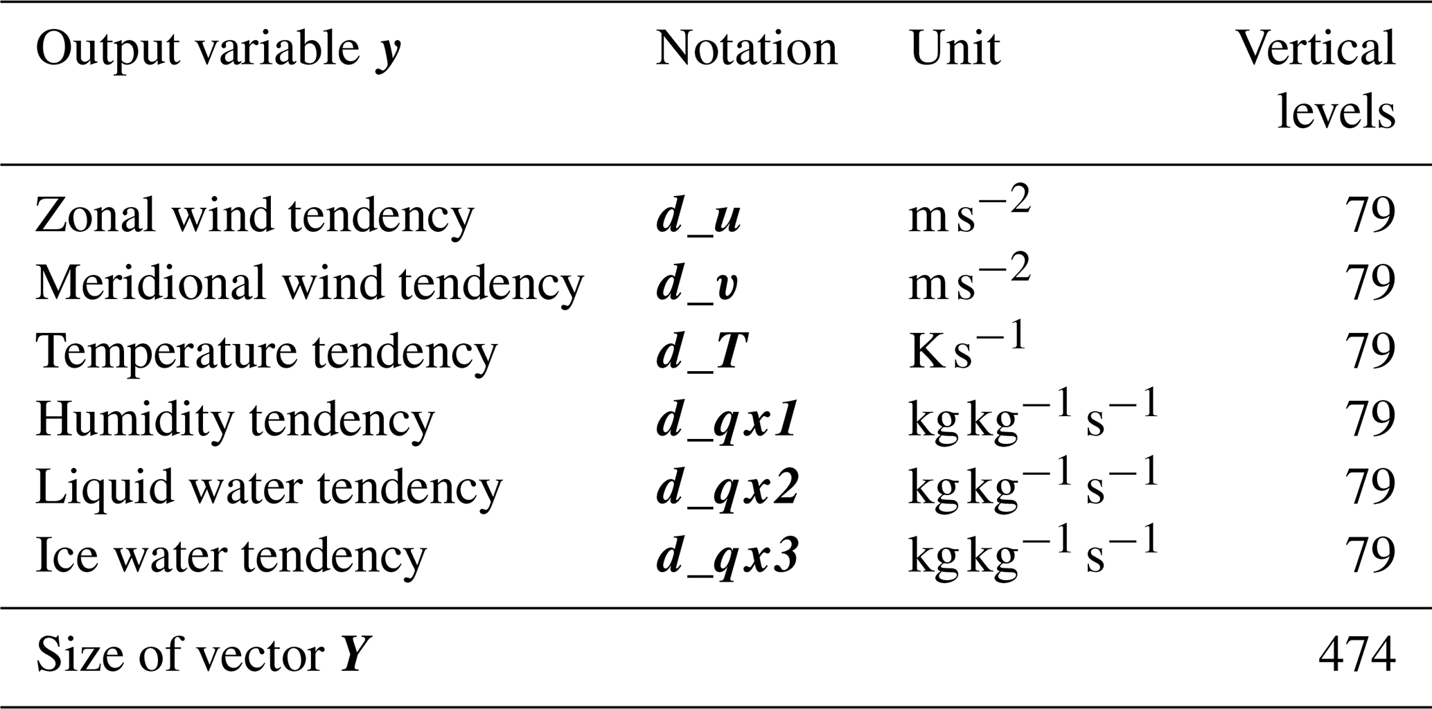
The outputs – also referred to as predictands or targets – consist of six vectors, each with a length of 79. These vectors represent profiles of the physical tendencies of the zonal wind d_u, the meridional wind d_v, the temperature d_T, the humidity d_qx1, the liquid water d_qx2 and the ice water d_qx3. All of these variables, listed in Table 2, are stacked in an output vector Y which has a length of 474 and is:

$$\mathit{Y}=\left[\mathit{d}\mathit{\_}\mathit{u},\mathit{d}\mathit{\_}\mathit{v},\mathit{d}\mathit{\_}\mathit{T},\mathit{d}\mathit{\_}\mathit{q}\mathit{x}\mathit{1},\mathit{d}\mathit{\_}\mathit{q}\mathit{x}\mathit{2},\mathit{d}\mathit{\_}\mathit{q}\mathit{x}\mathit{3}\right].$$

Table 2 List of output variables y for NNs.

2.3 Preprocessing

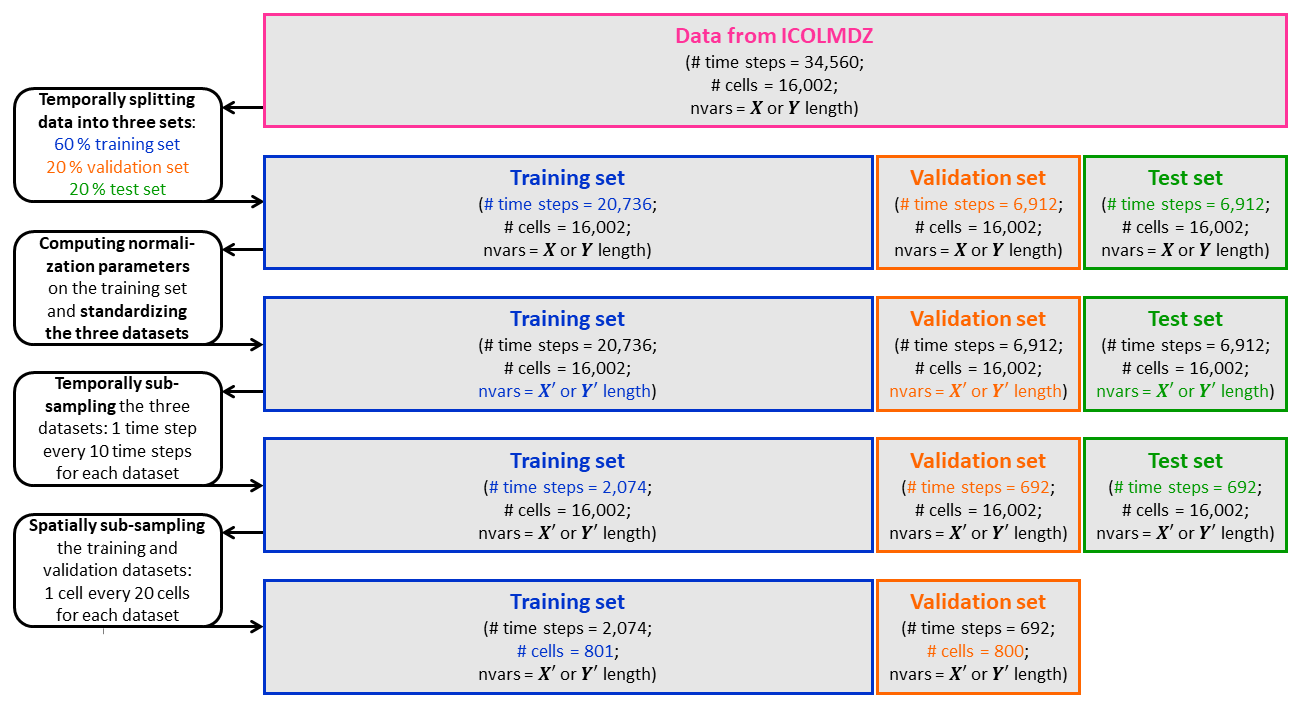
Data preprocessing is a crucial step in any ML process. It involves a series of essential tasks, which will be described in more detail in the following (see Fig. 2). The first step of preprocessing involves creating three datasets from our data. A training set is used for training the NN model by allowing it to learn patterns and relationships in the data, and optimize its parameters; a validation set helps prevent overfitting by evaluating how the model performs on unseen data; and a test set, used after training and validation, provides a final evaluation of the performance of the model. To create these three datasets, we have split the data by selecting a percentage of data in the time dimension. We can adopt the following data segmentation since we do not have a seasonal cycle in our aquaplanet simulation. The first 60 % correspond to the training dataset, the next 20 % are used to create the validation dataset, and finally, the test dataset contains the remaining 20 %. Thus, we obtain three datasets with 20 736 time steps for the training dataset and 6912 time steps for the other two datasets. This temporal segmentation is also adopted for the realistic experiment despite the active seasonal cycle.

Figure 2 Diagram of the data preprocessing steps.

Then, in order to ensure that all features have an equal influence in the training process and also to improve the performance and stability of the emulator during this process, we standardized the inputs and outputs so that all variables are on the same scale. To achieve this, let us consider a three-dimensional input variable x from the training dataset. We first calculated the mean μ_z(x^train) at each vertical level such as:

$$\begin{array}{}\text{(2)}& {\mathit{\mu }}_z\left({\mathit{x}}^{\text{train}}\right)={\displaystyle \frac{\mathrm{1}}{N_t{N}_i}}\sum _{t=\mathrm{1}}^{N_t}\sum _{i=\mathrm{1}}^{N_i}{\mathit{x}}_{t,i,z}^{\text{train}}\end{array}$$

where the index t indicates the time step, i denotes the horizontal grid point and z represents the vertical level. The variable ${\mathit{x}}_{t,i,z}^{\text{train}}$ corresponds to the value of x in the training dataset at time step t, horizontal grid point i and vertical level z. N_t and N_i are respectively the total numbers of time steps and horizontal grid points in the training dataset. The standard deviation σ(x^train) was also calculated on the training dataset on all time steps and grid points, across the entire vertical column, for each variable. The variance is not calculated for each level like μ_z(x^train) to avoid giving disproportionate weight to levels with low variance. The standard deviation can be expressed by the following:

$$\begin{array}{}\text{(3)}& \mathit{\sigma }\left({\mathit{x}}^{\text{train}}\right)=\sqrt{{\displaystyle \frac{\mathrm{1}}{N_t{N}_i{N}_z}}\sum _{t=\mathrm{1}}^{N_t}\sum _{i=\mathrm{1}}^{N_i}\sum _{z=\mathrm{1}}^{N_z}({\mathit{x}}_{t,i,z}^{\text{train}}-{\mathit{\mu }}_z({\mathit{x}}^{\text{train}}){)}^{\mathrm{2}}}\end{array}$$

here N_z is the total number of vertical levels. Once these parameters are calculated, we subtract the mean of the corresponding vertical level and divide by the standard deviation, for each variable at each vertical level in each dataset. This leads to training data with a mean of 0 and a standard deviation of 1. Therefore, the standardization of the input variable x, regardless of the dataset, can be written as:

$$\begin{array}{}\text{(4)}& {\mathit{x}}_{t,i,z}^{\prime }={\displaystyle \frac{{\mathit{x}}_{t,i,z}-{\mathit{\mu }}_z\left({\mathit{x}}^{\text{train}}\right)}{\mathit{\sigma }\left({\mathit{x}}^{\text{train}}\right)}}.\end{array}$$

Regarding the three scalar predictors that have no dependency on the vertical, the following standardization is applied:

$$\begin{array}{}\text{(5)}& {\mathit{x}}_{t,i}^{\prime }={\displaystyle \frac{{\mathit{x}}_{t,i}-\mathit{\mu }\left({\mathit{x}}^{\text{train}}\right)}{\mathit{\sigma }\left({\mathit{x}}^{\text{train}}\right)}}\end{array}$$

with parameters $\mathit{\mu }\left({\mathit{x}}^{\text{train}}\right)=\frac{\mathrm{1}}{N_t{N}_i}{\sum }_{t=\mathrm{1}}^{N_t}{\sum }_{i=\mathrm{1}}^{N_i}{\mathit{x}}_{t,i}^{\text{train}}$ and
$\mathit{\sigma }\left({\mathit{x}}^{\text{train}}\right)=\sqrt{\frac{\mathrm{1}}{N_t{N}_i}{\sum }_{t=\mathrm{1}}^{N_t}{\sum }_{i=\mathrm{1}}^{N_i}({\mathit{x}}_{t,i}^{\text{train}}-\mathit{\mu }({\mathit{x}}^{\text{train}}){)}^{\mathrm{2}}}$. As we are in the case of multivariate emulation, it is necessary to normalize the outputs. Equation (4) is thus also applied to the six three-dimensional output variables y with the appropriate parameters calculated using Eqs. (2) and (3). Once these preprocessing steps have been completed, standardized vectors X^′ and Y^′ are used.

We then perform temporal and spatial sub-sampling of the datasets to avoid spatio-temporal correlations and to reduce the cost of training. For this purpose, starting from the first time step for each dataset, we select one data point every ten time steps and thus obtain datasets with 2074 time steps for the training dataset and 692 time steps for the validation and test datasets. Moreover, we choose to take one cell every twenty cells to create the final training and validation datasets. In this way, we obtain data that is well distributed across the globe and we ensure that we have sampled at all latitudes (see Fig. S1 in the Supplement). Finally, the training dataset contains data from 801 cells and the validation dataset has 800 cells spread across the globe among the 16 002 cells. We took care to ensure that this spatial selection represented all the regions. Therefore, we have 1 661 274 samples (2074×801 grid points) for the training dataset. We validate our models on a dataset with 553 600 samples (692×800 grid points). In order to study the results of the emulators across all grid cells of the globe, the temporal sub-sampling has not been applied for the test dataset.

3 Methods

3.1 Neural network architectures

An ML emulator estimates the output variables ${\widehat{\mathit{Y}}}^{\prime }$ from predictors X^′ which have corresponding outputs Y^′ in the dataset, using a function denoted $\widehat{f}$, such as ${\widehat{\mathit{Y}}}^{\prime }=\widehat{f}({\mathit{X}}^{\prime },\mathit{\theta })$ where $\mathit{\theta }=(\mathbf{w},\mathit{b})$ with w the weights and b the biases. Therefore, the goal of NNs during training is to minimize the error between prediction ${\widehat{\mathit{Y}}}^{\prime }$ and reference data Y^′. In other words, the objective is to optimize the function $\mathcal{L}({\mathit{Y}}^{\prime },{\widehat{\mathit{Y}}}^{\prime })$ – referred to as the loss function in ML jargon – by updating the weights and biases of the model iteratively (LeCun et al., 2015). The challenge with a ML model is to find a balance between underfitting and overfitting. The first one occurs when the correlations in the training data are not captured by the predictive model because it is inappropriate. The second one arises when the predictive model fits the training data well, and fails to generalise to data that it has not yet seen during the training process. In other words, the model captures the correlations but also the noise produced by the training dataset (Goodfellow et al., 2016).

We want to develop an emulator encompassing all the physics of our standard model; its role is to provide predictions of the subgrid physical tendencies for each level of each atmospheric column at every time step. To this end, we have investigated and implemented several NN-based emulators using the Keras API (Chollet, 2015) and TensorFlow framework (Abadi et al., 2015). These include DNNs (Goodfellow et al., 2016), Convolutional Neural Networks (CNNs) (LeCun et al., 1990), U-Nets (Ronneberger et al., 2015), and U-Nets with ResBlocks (He et al., 2015). For these emulators, the hyperparameters were selected based on preliminary tests. Adam is the optimization algorithm chosen for gradient descent, which allows the weights to be updated iteratively and helps find the optimal values for these parameters. For each NN model, the input vector X^′ passes through a first input layer. The last layer corresponds to a dense layer with a size of the output vector Y^′. This last layer has no activation function due to the nature of the problem, which is a regression task. Below, we will provide descriptions only of a DNN model and a U-Net model with residual blocks, as these are the two models that will be studied throughout the rest of the article. It should be noted that many different setups for the DNN but also for the U-Net have been tested, but we chose to work with models offering a good trade-off between the computation time and the quality of the results.

The first architecture we use is a DNN which consists of a succession of dense layers described in Table S1 in the Supplement. It is composed by six connected hidden layers of 512 neurons each, with a full connectivity between adjacent layers. The activation function of the hidden layers is Rectified Linear Unit (ReLU) (Glorot et al., 2011; LeCun et al., 2015). It is trained with a learning rate of 10⁻³, and the batch size is equal to 64. This neural network contains around 2 million parameters.

We have also used a specific architecture, called a U-Net model (Ronneberger et al., 2015), where we use 1D convolutional layers. This model has the advantage of learning features at multiple scales and capturing spatial dependencies between features through a series of convolution operations. It is known for its encoder-decoder structure, featuring a dual-path design: a down-sampling side for capturing contextual information by reducing spatial resolution, and an up-sampling side for achieving precise localization by increasing the resolution. For a given resolution, the encoding and decoding parts are linked with skip connections, and at the lowest resolution, these parts are connected via a bottleneck layer. Combined with this u-shaped architecture, ResBlocks have been included in this model whose aim is to predict the errors – or residuals – made by the model. Indeed, these blocks allow gradients to propagate more effectively during backpropagation, resulting in better convergence. In the Supplement, Fig. S2 gives a schematic description of the 1D U-Net architecture built and Table S2 in the Supplement summarizes the layers. The temporal and spatial dimensions of data are merged before data is fed into this NN. The reverse operation if performed at the output. At the input, the three scalars are separated from the vectors in order to extend them across all vertical levels, and then concatenated with the other vector variables, so they can be integrated during the convolutional layers. Data is reformatted before being provided to the encoder. For vectors, but also the three scalars spread across all vertical levels, we concatenate each atmospheric column in order to obtain a 2D matrix of dimension 79 multiplied by the number of 1D variables. This data format is compatible with the 1D convolution operator that processes each atmospheric column independently. At the output stage, a 1D convolutional layer and a reshape layer are used to transform the data back into a vector format. The learning rate is set at 10⁻³, and the batch size equals to 64. This model has around 13 million parameters.

Each emulator is trained for a certain number of epochs, with each epoch representing a complete pass of the training dataset through the algorithm. To evaluate the performance of emulators during training, the output tendencies from the NNs are compared with those from ICOLMDZ. The quantification of the difference between the NNs predictions and the reference data in the training dataset is done using a loss function ℒ. We have selected the Mean Squared Error (MSE), commonly used in regression problems, as the loss function. MSE is sensitive to outliers since large errors are penalized much more than smaller ones. It is defined as follows:

$$\begin{array}{}\text{(6)}& \text{MSE}({\mathit{Y}}^{\prime },{\widehat{\mathit{Y}}}^{\prime })={\displaystyle \frac{\mathrm{1}}{N}}\sum _{j=\mathrm{1}}^N\Vert {\mathit{Y}}_j^{\prime }-{\widehat{\mathit{Y}}}_j^{\prime }{\Vert }^{\mathrm{2}}\end{array}$$

where $\Vert .{\Vert }_{\mathrm{2}}$ denotes the Euclidean norm, N is the total number of samples in the dataset, ${\mathit{Y}}_j^{\prime }$ the target and ${\widehat{\mathit{Y}}}_j^{\prime }$ the prediction for the jth value on the dataset. In our case, the loss function is computed directly on the standardized data, given that we are working in a multivariate setting. MSE is calculated on the training dataset but also on the validation dataset. Early stopping criterion has been used to prevent overfitting since this option monitors the performance of the model on a validation dataset during the training process. Thus, training is stopped when the performance on the validation set no longer improves. For this criterion, we set a patience of 20 epochs. It should be noted that this stopping criterion may prevent models from converging perfectly, the key point is to avoid overfitting. Thus, the models saved and used are those that achieved the best performance according to the computed loss metric on the validation dataset tracked during training. In the following sections, the predictive performance of the DNN and the U-Net described above will be compared. Each model has been trained a few times, but as we observed similar behaviours and performance in terms of loss function for a chosen model, we only kept one of each.

3.2 Evaluation metrics

After the learning process is completed and the parameters have been set, the final evaluation is done on the test dataset. We evaluate the offline performance of our emulator with different statistical indicators for each physical tendency that has been previously denormalized. Firstly, to perform a one-dimensional analysis of the results, we synthesized temporal and spatial information by computing statistics on all time steps and grid points. This gives an initial overview of the results of an emulator despite the spatio-temporal complexity of the problem. We calculate the global mean and the global variance of the six physical tendencies separately for each vertical level, over all time steps and all grid points combined. These metrics are applied to both the reference tendencies Y from the ICOLMDZ simulation and the predicted tendencies $\widehat{\mathit{Y}}$, in order to compare them. If we consider a reference physical tendency noted y from the test subset, then its global mean μ_z(y^test) at vertical level z is expressed as:

$$\begin{array}{}\text{(7)}& {\mathit{\mu }}_z\left({\mathit{y}}^{\text{test}}\right)={\displaystyle \frac{\mathrm{1}}{N_t{N}_i}}\sum _{t=\mathrm{1}}^{N_t}\sum _{i=\mathrm{1}}^{N_i}{\mathit{y}}_{t,i,z}^{\text{test}}\end{array}$$

where N_t and N_i are respectively the total numbers of time steps and grid points in the test dataset. The term ${\mathit{y}}_{t,i,z}^{\text{test}}$ include data for all time steps, grid points and vertical levels. The global variance ${\mathit{\sigma }}_z^{\mathrm{2}}\left({\mathit{y}}^{\text{test}}\right)$ of this physical tendency y is given as follows:

$$\begin{array}{}\text{(8)}& {\mathit{\sigma }}_z^{\mathrm{2}}\left({\mathit{y}}^{\text{test}}\right)={\displaystyle \frac{\mathrm{1}}{N_t{N}_i}}\sum _{t=\mathrm{1}}^{N_t}\sum _{i=\mathrm{1}}^{N_i}{\left({\mathit{y}}_{t,i,z}^{\text{test}}-{\mathit{\mu }}_z\left({\mathit{y}}^{\text{test}}\right)\right)}^{\mathrm{2}}.\end{array}$$

These two metrics are calculated for each vertical level, allowing us to examine the global vertical profiles of the mean and the variance of the tendency y. Equations (7) and (8) are also applied to each predicted physical tendency $\widehat{\mathit{y}}$ to compare their results with those of y, providing a first overall assessment of the emulator studied.

Moreover, we used two metrics for each tendency separately over all time steps, cells and vertical levels to assess the general performance of an emulator. Firstly, the coefficient of determination, denoted R², is defined as follows:

$$\begin{array}{}\text{(9)}& {\displaystyle }{R}^{\mathrm{2}}\left({\widehat{\mathit{y}}}^{\text{test}}\right)& {\displaystyle }=\mathrm{1}-{\displaystyle \frac{{\displaystyle }\text{MSE}({\mathit{y}}^{\text{test}},{\widehat{\mathit{y}}}^{\text{test}})}{{\displaystyle }\text{MSE}({\mathit{y}}^{\text{test}},\mathit{\mu }({\mathit{y}}^{\text{test}}\left)\right)}}\text{(10)}& {\displaystyle }& {\displaystyle }=\mathrm{1}-{\displaystyle \frac{{\displaystyle }\sum _{t=\mathrm{1}}^{N_t}{\sum }_{i=\mathrm{1}}^{N_i}{\sum }_{z=\mathrm{1}}^{N_z}{\left({\mathit{y}}_{t,i,z}^{\text{test}}-{\widehat{\mathit{y}}}_{t,i,z}^{\text{test}}\right)}^{\mathrm{2}}}{{\displaystyle }\sum _{t=\mathrm{1}}^{N_t}{\sum }_{i=\mathrm{1}}^{N_i}{\sum }_{z=\mathrm{1}}^{N_z}{\left({\mathit{y}}_{t,i,z}^{\text{test}}-\mathit{\mu }\left({\mathit{y}}^{\text{test}}\right)\right)}^{\mathrm{2}}}}\end{array}$$

where N_z corresponds to the 79 vertical levels and μ(y^test) is the average of ${\mathit{y}}_{t,i,z}^{\text{test}}$. We have also calculated the global Root Mean Square Error (RMSE) which is:

$$\begin{array}{ll}{\displaystyle }\text{RMSE}& {\displaystyle }({\mathit{y}}^{\text{test}},{\widehat{\mathit{y}}}^{\text{test}})\\ \text{(11)}& {\displaystyle }& {\displaystyle }=\sqrt{\text{MSE}{\displaystyle }({\mathit{y}}^{\text{test}},{\widehat{\mathit{y}}}^{\text{test}})}\text{(12)}& {\displaystyle }& {\displaystyle }=\sqrt{{\displaystyle \frac{\mathrm{1}}{N_t{N}_i{N}_z}}\sum _{t=\mathrm{1}}^{N_t}\sum _{i=\mathrm{1}}^{N_i}\sum _{z=\mathrm{1}}^{N_z}({\mathit{y}}_{t,i,z}^{\text{test}}-{\widehat{\mathit{y}}}_{t,i,z}^{\text{test}}{)}^{\mathrm{2}}}.\end{array}$$

We will sometimes compute the RMSE on specific subsets of the test dataset to assess performances that vary for instance across latitudes or vertical levels.

4 Initial training performance with the aquaplanet setup

The emulation of the six physical tendencies is performed simultaneously. However, we will first focus on the results of the zonal wind tendency, noted as d_u, and then we will briefly analyze the other five tendencies, for which figures are provided in the Supplement.

4.1 Results

First, we examine the global vertical profiles of the mean (see Fig. 3a) and variance (see Fig. 3b) of the zonal wind tendency, to analyze the results obtained from our emulators with the test subset which contains the 16 002 cells. These profiles were created to bring both spatial and temporal information. Indeed, they were produced by averaging data over the whole globe and over all time steps that define the test subset. For the DNN, the predicted global mean profile of the zonal wind tendency shows a good overall agreement with the reference global mean between levels 25 and 79, even though the predicted curve does not perfectly match the reference curve. Indeed, the curve of the predicted global mean oscillates around the reference global mean. Below level 25, the global mean predicted using the emulator deviates significantly from the reference data. Moreover, the global variance is underestimated in the predictions, with a variance ranges from 0 to $\mathrm{2.7}\times {\mathrm{10}}^{-\mathrm{7}}$ m² s⁻⁴ – equivalent to a standard deviation ranges from 0 to $\mathrm{5.2}\times {\mathrm{10}}^{-\mathrm{4}}$ m s⁻² –, compared to that of the reference data, whose variance is between 0 and $\mathrm{4.5}\times {\mathrm{10}}^{-\mathrm{7}}$ m² s⁻⁴ – i.e. a standard deviation ranges from 0 to $\mathrm{6.7}\times {\mathrm{10}}^{-\mathrm{4}}$ m s⁻². This is particularly notable at lower vertical levels between levels 0 and 10 where there is higher variability in the reference data, posing a challenge for the emulator. As a result, while the emulator can predict the zonal wind tendency reasonably well on average, it struggles to capture extreme values. For the U-Net, the predicted global mean profile is smoother and aligns closely with the reference global mean profile except for the very first levels. The predicted variance ranges from 0 to $\mathrm{3.5}\times {\mathrm{10}}^{-\mathrm{7}}$ m² s⁻⁴. It is similar to the reference variance for vertical levels above 30 but, like the DNN, the predicted global variance profile is underestimated between levels 0 and 25. However, on the other hand, when comparing the results obtained from both the DNN and the U-Net, we can highlight that the U-Net model produces better predictions than the DNN, whether in terms of global mean or global variance. These results lead us to explore the factors contributing to make the U-Net more effective and accurate than the DNN, as well as the reasons behind the underestimation of the variance from the DNN.

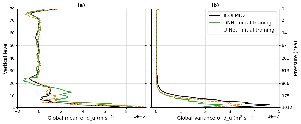
Figure 3 Global vertical profiles of the zonal wind tendency d_u of the mean (a) and the variance (b) for the test subset, obtained with the initial training. In these panels, the black curves represent the reference data from the ICOLMDZ simulation. The green curves correspond to predictions made by the DNN while the dashed orange curves represent the results obtained using the U-Net.

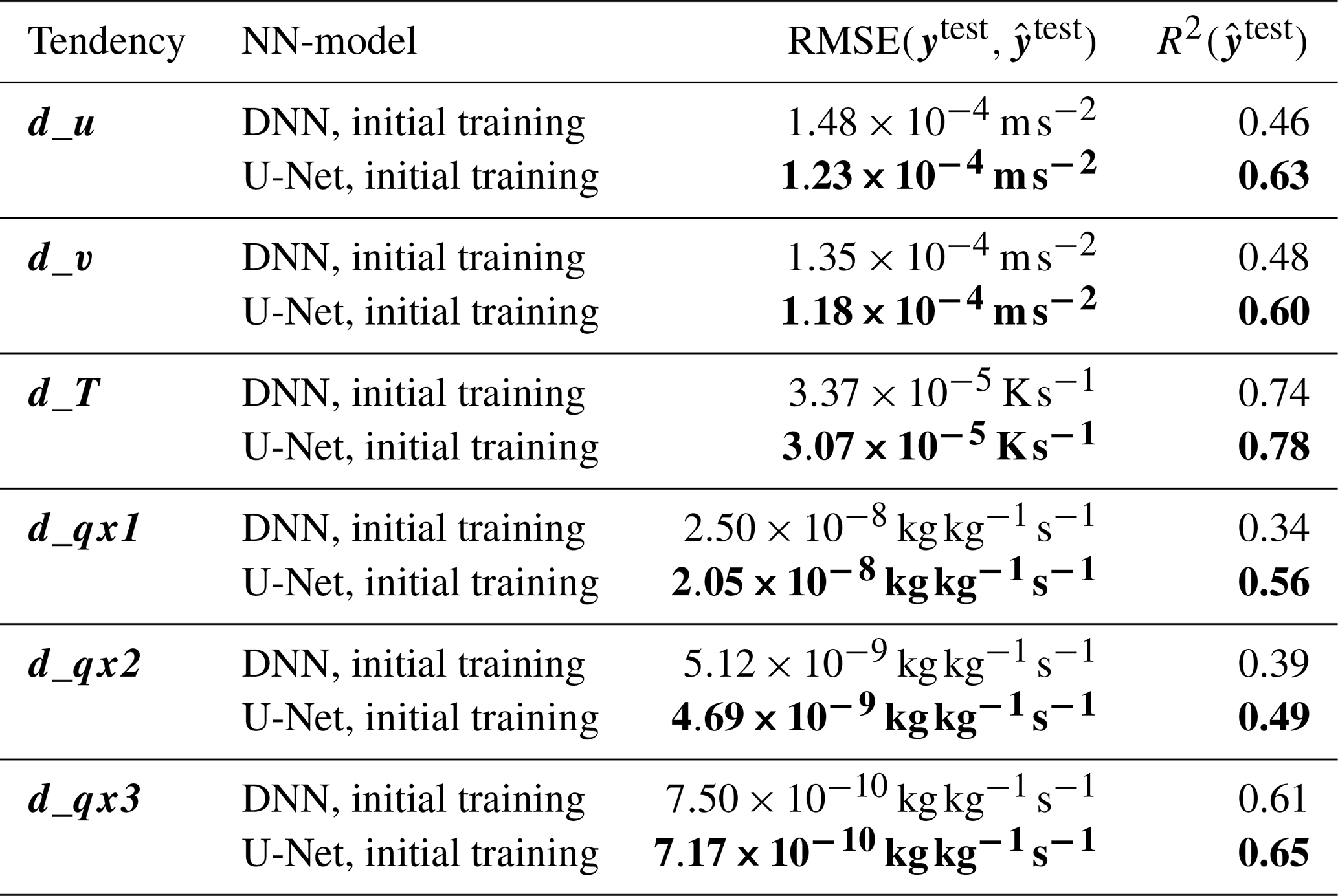
We compute some general statistical indicators to evaluate the global performance of the emulators in reproducing the zonal wind tendency d_u. Table 3 shows the results. By comparing the global RMSE of the DNN and the U-Net, we observe that the DNN has a RMSE of $\mathrm{1.48}\times {\mathrm{10}}^{-\mathrm{4}}$ m s⁻² and that of the U-Net is equal to $\mathrm{1.23}\times {\mathrm{10}}^{-\mathrm{4}}$ m s⁻². Therefore, with a global RMSE approximately 16.9 % lower than that of the DNN, the U-Net architecture outperforms the DNN. This statement can also be made based on the results of the coefficient of determination. This metric is equal to 0.63 for the U-Net, whereas it equals 0.46 for the DNN. This confirms that the DNN captures less variance than the U-Net model. Therefore, the U-Net architecture presents better skills at predicting the zonal wind tendency.

Table 3 Results of the general metrics for the six tendencies over all time steps, cells and vertical levels of the test subset, to evaluate the two initial emulators studied. The best metric values for each tendency are shown in bold.

We have calculated the zonal RMSE of the zonal wind tendency for the DNN and the U-Net in order to study the dependence of this metric on altitude and latitude (see Fig. 4a and b). The first notable observation, regardless of the emulator, is the North-South symmetry which is expected in our context as we study an aquaplanet with a constant equinox without seasonal cycle. Then, the results highlight the fact that both emulators exhibit a significantly higher zonal RMSE of the zonal wind tendency – equal to $\mathrm{5.0}\times {\mathrm{10}}^{-\mathrm{4}}$ m s⁻² – in the first 10 vertical levels. These results align with the global vertical profiles of the variance analyzed previously, since it is at these vertical levels that the variability of the zonal wind tendency is most pronounced. Moreover, we see that emulators perform better in some regions, particularly near the equator and at high latitudes – above 60° S and 60° N – compared to the mid-latitudes – between 30 and 60° S and between 30 and 60° N. However, the U-Net architecture performs better, as the pattern of high zonal RMSE is less widespread, especially at high latitudes around 60° S and 60° N. For each emulator, we observe quite similar patterns for the levels below 40, with a zonal RMSE around $\mathrm{1.5}\times {\mathrm{10}}^{-\mathrm{4}}$ m s⁻², mainly pronounced from latitudes 30° S and 30° N to the poles. The metric studied is weak above vertical level 40 at all latitudes. Indeed, neither emulator seems to be better at these vertical levels, particularly with regard to the representation of variance and this result can be seen in the zonal RMSE. This poses a need to further investigate and examine the results of the emulation by latitude bands, particularly between latitudes 30 and 60° in each hemisphere, in the first vertical levels.

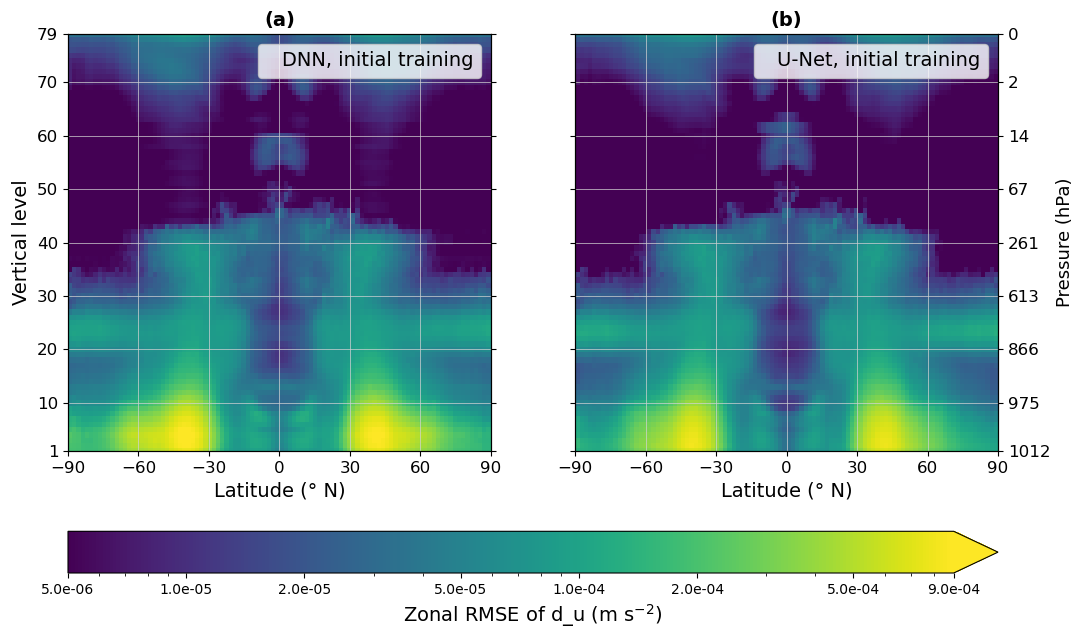
Figure 4 Cross-sections of the zonal RMSE of the zonal wind tendency d_u for the test subset, from the DNN (a) and from the U-Net (b) with the initial approach. The colorbar displays data on a logarithmic scale.

4.2 Study by latitude bands

To better understand the results of the emulators, we examine them by latitude belts, as the zonal wind tendency is the result of various physical processes that do not operate in the same way across regions. For this spatial study, we defined three latitude intervals for which global mean and variance profiles of the zonal wind tendency are calculated (Fig. 5). The first one covers the tropics, i.e. for data with a latitude, noted ϕ, in the range [25° S,25° N] (see Fig. 5a and b). The second interval corresponds to the subtropical regions which are defined by the union of two latitude intervals such that $[\mathrm{45}\mathit{°}\mathrm{S},\mathrm{25}\mathit{°}\mathrm{S}[\cup ]\mathrm{25}\mathit{°}\mathrm{N},\mathrm{45}\mathit{°}\mathrm{N}]$ (see Fig. 5c and d). Finally, the high latitudes are represented by the third interval which is $[\mathrm{90}\mathit{°}\mathrm{S},\mathrm{45}\mathit{°}\mathrm{S}[\cup ]\mathrm{45}\mathit{°}\mathrm{N},\mathrm{90}\mathit{°}\mathrm{N}]$ (see Fig. 5e and f). As shown in Fig. 5a, c, and e, mean profiles are very different from one latitude band to another. These figures illustrate that, regardless of the network used, the emulators provide a good representation of the global mean of the zonal wind tendency across latitude bands. The predicted profiles do not correspond exactly to the profiles of the reference data. Nevertheless, they tend to follow the overall behaviour of the global means of the zonal wind tendency. In the tropics, both emulators struggle more in the first vertical levels as well as in the upper layers of the atmosphere as shown in Fig. 5a. Regarding the other two latitude bands, the emulators face some difficulties in the lower vertical levels (see Fig. 5c and e). As shown in Fig. 5d, the vast majority of the zonal wind tendency variability comes from extratropical regions, especially subtropical areas, where the variance is particularly high in the first 10 levels. Indeed, the maximum variance is equal to $\mathrm{9.4}\times {\mathrm{10}}^{-\mathrm{7}}$ m² s⁻⁴ – equivalent to a maximum standard deviation of $\mathrm{9.7}\times {\mathrm{10}}^{-\mathrm{4}}$ m s⁻² – whereas in the tropics (see Fig. 5b) this maximum is around $\mathrm{1.6}\times {\mathrm{10}}^{-\mathrm{8}}$ m² s⁻⁴ – which corresponds to a maximum standard deviation of $\mathrm{1.3}\times {\mathrm{10}}^{-\mathrm{4}}$ m s⁻². The high latitudes (see Fig. 5f) also show considerable variability, with a maximum variance of $\mathrm{6.4}\times {\mathrm{10}}^{-\mathrm{7}}$ m² s⁻⁴ – i.e. a maximum standard deviation of $\mathrm{8.0}\times {\mathrm{10}}^{-\mathrm{4}}$ m s⁻². Above level 20, the variance for the three latitude bands appears to approach 0. Whatever the study area, the variances from the two emulators do not reach the variance of the reference data, but the U-Net model performs better than DNN. This raises the question of the origins of this underestimation of the variance. We know that physical phenomena, such as convection and turbulence, manifest differently depending on the latitudes. Therefore, this leads us to question and investigate the underlying physical mechanisms responsible for the significant variance, which is further discussed in Sect. 5.

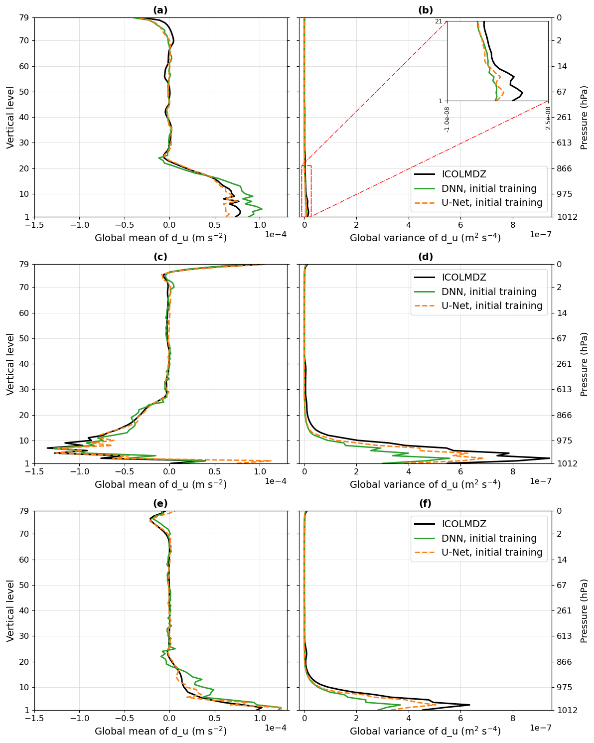
Figure 5 Global vertical profiles of the zonal wind tendency d_u of the mean (a, c, e) and the variance (b, d, f) for the test subset, obtained with the initial approach. Panels (a) and (b) correspond to the tropics ($\mathit{\varphi }\in [\mathrm{25}\mathit{°}\mathrm{S};\mathrm{25}\mathit{°}\mathrm{N}]$), panels (c) and (d) represent the subtropical regions ($\mathit{\varphi }\in [\mathrm{45}\mathit{°}\mathrm{S},\mathrm{25}\mathit{°}\mathrm{S}[\cup ]\mathrm{25}\mathit{°}\mathrm{N},\mathrm{45}\mathit{°}\mathrm{N}]$) and panels (e) and (f) are the high latitudes ($\mathit{\varphi }\in [\mathrm{90}\mathit{°}\mathrm{S},\mathrm{45}\mathit{°}\mathrm{S}[\cup ]\mathrm{45}\mathit{°}\mathrm{N};\mathrm{90}\mathit{°}\mathrm{N}]$). The data from the ICOLMDZ simulation are represented by the black curves. The green curves come from the DNN and the dashed orange curves represent the U-Net, for the initial training.

4.3 Results on the other five tendencies

After focusing on the zonal wind tendency, we can now discuss the ability of the emulators to reproduce the other five tendencies: the meridional wind, temperature, humidity, liquid water and ice water tendencies. The zonal wind tendency and these five tendencies are emulated simultaneously. Firstly, the results of the global metrics for these five tendencies (see Table 3) show systematically better scores with the use of the U-Net model compared to the DNN. The global vertical profiles (Fig. S6a and b for d_v, Fig. S10a and b for d_T, Fig. S14a and b for d_qx1, Fig. S18a and b for d_qx2, Fig. S22a and b for d_qx3) and the cross-sections of the zonal RMSE (Fig. S7a and b for d_v, Fig. S11a and b for d_T, Fig. S15a and b for d_qx1, Fig. S19a and b for d_qx2, Fig. S23a and b for d_qx3) of these tendencies are presented in the Supplement.

The comparison of the global vertical profiles of the mean of these five tendencies and the zonal wind tendency (see Figs. 3a, S6a, S10a, S14a, S18a and S22a) highlights the fact that the tendencies do not have the same vertical structures. This is due to different physical processes which are active at different altitudes. For each tendency, we can provide a physical interpretation of its global vertical profile of the mean. Overall the meridional wind tendency is close to 0 along the vertical as all physical processes balance and do not have preferential direction. At the bottom of the atmosphere, the temperature tendency is positive mainly due to turbulence, thermals and large scale condensation, and to a lesser extent, to convection and longwave radiation. Then, this tendency decreases with altitude until the tropopause, around level 40. For the first vertical levels, the humidity tendency is positive due to various physical processes such as turbulence, thermals, evaporation and large scale condensation for instance. In the lower atmosphere, the liquid water tendency is positive due to large scale condensation processes. However, the humidity and liquid water tendencies decrease with altitude. Between vertical levels 25 and 35, these tendencies are negative because the water precipitates or solidifies. This explains why, for these same vertical levels, the solid water tendency increases. Then, this tendency becomes negative with the sedimentation process. Above the tropopause, the three water tendencies are close to 0 due to the temperature and pressure conditions.

Nevertheless, the overall conclusion is the same for all the tendencies: where the variability of the tendency studied is the highest (see Figs. 3b, S6b, S10b, S14b, S18b and S22b), usually at the bottom of the atmosphere, emulators struggle to represent the global mean correctly. As was the case with the zonal wind tendency, the U-Net architecture has a better ability to capture the reference tendencies than the DNN. The global mean curves are sometimes smoother for the U-Net than the DNN. Moreover, the representation of the global variance is always underestimated by both emulators, especially where the variance is strongest, whatever the tendency studied. However, this behaviour is even more pronounced with the DNN and the U-Net demonstrates better performances in capturing the variability of the tendency studied. Some specific features of each tendency can be discussed. From the surface to level 20, the global mean of the reference meridional wind tendency presents some oscillations around 0. For the same levels, the DNN tends to underestimate this global mean, whereas in the upper of the atmosphere, both emulators overestimate the global mean and the variance is not captured at all. Above level 20 for the meridional wind tendency and level 40 for the humidity, liquid water tracer and ice water tracer tendencies, the global means of the reference data appear to remain close to 0. The global means predicted by the two emulators, for each tendency, are quite unstable and oscillate around the reference data. While the global mean of the DNN fluctuates between negative and positive values around the reference global mean, the U-Net is quite close to the reference data, but overestimates it. This highlights the challenges faced by the emulator. The global variance of the ice water tracer tendency is quite well represented with both emulators, despite a slight underestimation compared with the reference curve. For the temperature tendency, the DNN underestimates the global mean, while the U-Net, despite its overestimation at high altitudes, appears to be slightly closer to the global mean especially at the bottom of the atmosphere. The performances of the DNN and the U-Net architecture in terms of reproducing variability are quite similar and reveal to be quite accurate. However, the U-Net seems to be slightly better in general, except at the variance peak around the 70th vertical level.

Finally, the cross-sections of the zonal RMSE of the five tendencies show similar results to the cross-sections of the zonal RMSE of the zonal wind tendency discussed previously (see Figs. 4a and b, S7a and b, S11a and b, S15a and b, S19a and b and S23a and b). For a chosen tendency, even if the region where the highest zonal RMSE is the same for both emulators, we see that the RMSE values are more pronounced with the DNN, as the region is much larger than for the U-Net. However, the location of this pattern depends on the tendency. For the meridional wind tendency, it is at the same latitudes and vertical levels as the zonal wind tendency, but, we observe an additional pattern at the top of the atmosphere between 30 and 60° in each hemisphere. For the temperature, humidity and liquid water tendencies, we see that the zonal RMSE is high for latitudes between 55° S and 55° N, and for vertical levels below 30. Concerning the solid water tendency, there is a pattern with a high zonal RMSE defined between levels 20 and 40 for latitudes from 30° to the pole in each hemisphere.

Therefore, this brings us to consider two key points: the potential factors that may be responsible for the underestimation of the variance with both emulators, and also, what might explain the better performance of the U-Net compared to the DNN.

5 Refined approach for the aquaplanet setup: integrating physical knowledge

In this section, we analyze the physical phenomena that could be the cause of lower performance with the DNN compared to the U-Net and we provide new predictors in addition to those already used as input in our emulators in an attempt to improve the results of our DNN.

5.1 Breakdown of tendencies into physical processes

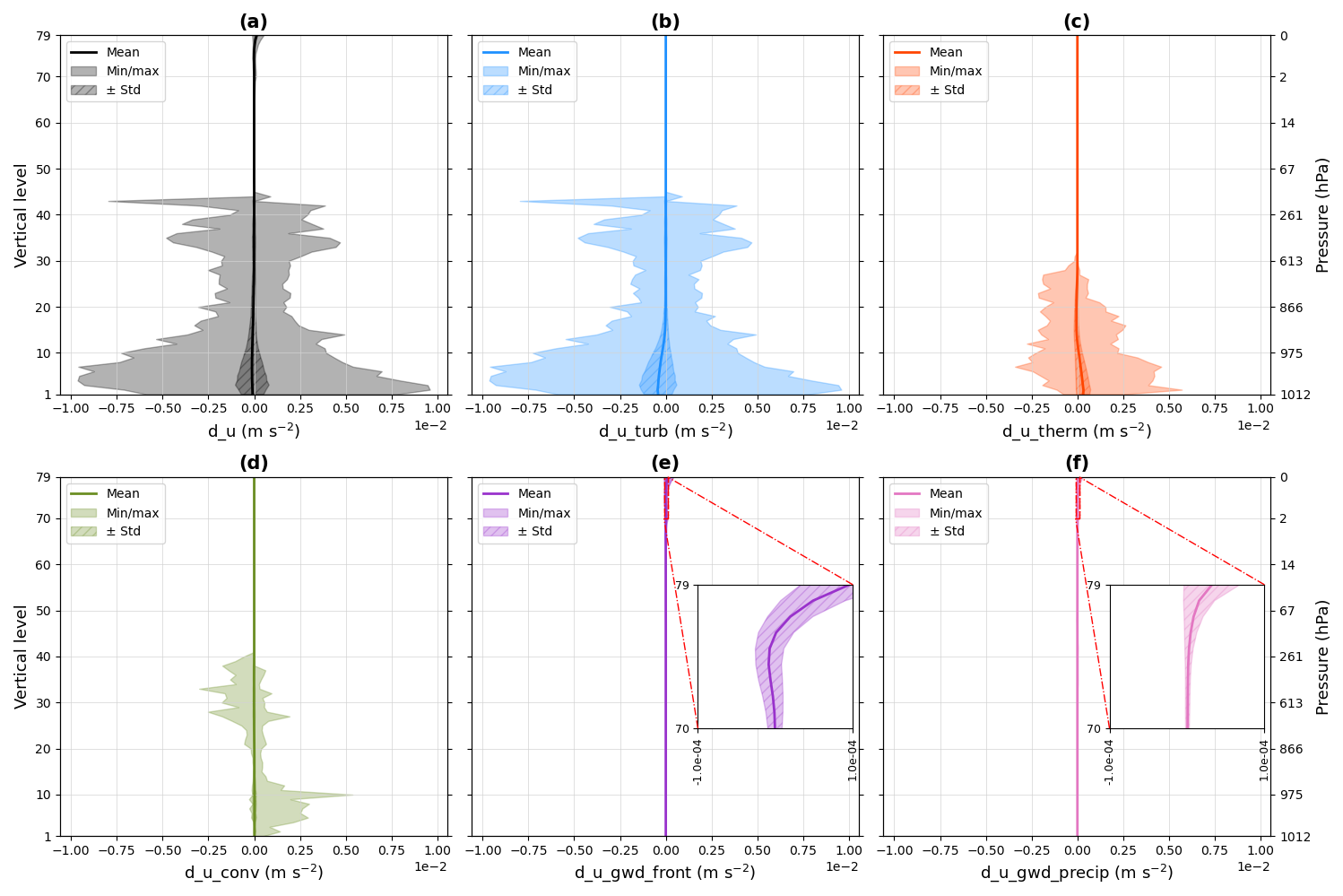
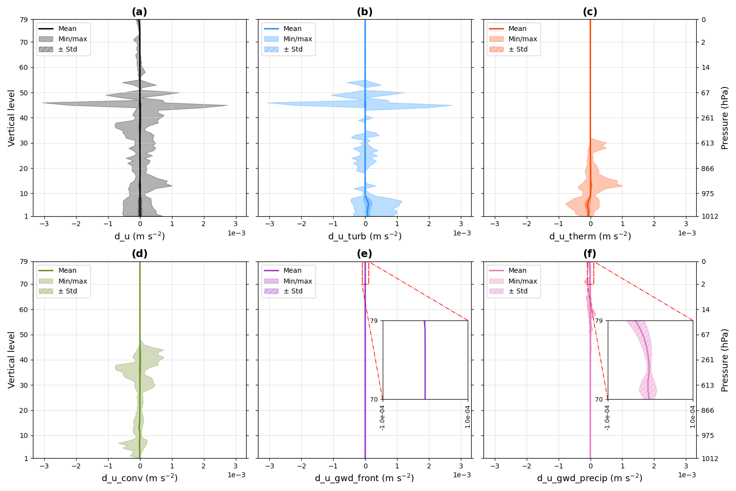
To understand the underestimation of the variance and its physical origin, we break down the zonal wind tendency into physical phenomena included in its computation within phyLMDZ. As mentioned above, in this model each tendency is the sum of various tendencies due to different physical processes (see Eq. 1). We decided to carry out this study on three columns – noted A, B and C – located in different regions of the globe to examine the contribution of each phenomenon. We define a first point located at high latitudes (ϕ_A=78.5° N; λ_A=7.86° E), another in the subtropics (ϕ_B=33.2° N; λ_B=70.2° E) and a last one near the equator (ϕ_C=0.413° N; λ_C=48.6° E).

To provide a comparison between the three cells, we investigate their vertical profiles from a randomly chosen time step as shown in the Supplement for A (Fig. S3), B (Fig. S4) and C (Fig. S5). The vertical profiles are those of the total zonal wind tendency and also those of the physical processes that contribute to and influence this total tendency. These physical processes include turbulence d_u_turb, boundary-layer convection d_u_therm, and convection modelled as static adjustment d_u_conv, gravity wave drag due to emission by fronts d_u_gwd_front and those due to emission by convective systems d_u_gwd_precip. Firstly, we can note that the scales of the zonal wind tendency signals differ among the three points (see Figs. S3a, S4a and S5a). This variation in scale highlights differences in intensity with latitude: the zonal wind tendency is highest in the subtropics (10⁻³ m s⁻²), lower in high latitudes (10⁻⁴ m s⁻²), and lowest near the equator (10⁻⁵ m s⁻²). However, by decomposing the vertical profile of the zonal wind tendency into vertical profiles of the various physical processes involved, we observe that these processes do not have the same influence depending on the point and so, on the latitude studied. Whatever the point considered, turbulent movements (see Figs. S3b, S4b and S5b) can be observed near the surface. These movements also occur at higher altitudes, more precisely between vertical levels 20 and 40, for the points located at high latitudes and in the subtropics. Turbulence is the physical process whose intensity is greatest for these two points. The contribution of thermals (see Figs. S3c, S4c and S5c) is located in the vertical levels below the 30th in high latitudes and especially at the equator. However, for the subtropics they have no impact on the total tendency. At high latitudes as in the subtropics, convection (see Figs. S3d, S4d and S5d) does not play a role, unlike at the equator where it is the physical process that makes the major contribution, particularly between vertical levels 20 and 40. Whatever the point studied, gravity wave drag linked to the fronts (see Figs. S3e, S4e and S5e) are only present at the top of the atmosphere. This is also the case for gravity wave drag from convective systems (see Figs. S3f, S4f and S5f) whose signal is much stronger at the point near the equator than at the other two points. Therefore, this approach shows that turbulence is the predominant physical process in subtropical regions (Fig. S4) and at high-latitude regions (Fig. S3), where the emulator capabilities are limited concerning the correct reproduction of the variability.

Based on a full-year simulation, we studied the mean vertical profiles of these three points for the total zonal wind tendency but also for the physical processes, shown in Fig. 6 for A, Fig. 7 for B and Fig. 8 for C. They include a minimum/maximum envelope that contains all the vertical profiles for the entire year, as well as a hatched area representing the standard deviation around the mean profile. The mean vertical profile of the total zonal wind tendency illustrated in Fig. 7a highlights that the average annual value is zero. Thus, all physical processes balance over a year. This result is also found for A and C. Whatever the cell studied, several points can be noted. Firstly, the majority of the total zonal wind tendency variability is located between the 1st and the 20th vertical level. This variability is higher for B than A, and higher for A than C. From the bottom of the atmosphere to vertical level 38, 45 or 65 – respectively for the point A, B or C – phenomena relating to turbulence, thermals and convection are present and contribute to the total zonal wind tendency. On the other hand, gravity wave drag occur at the top of the atmosphere with a lower amplitude than for the other physical processes. As the total tendency is the sum of the other tendencies, it is clear that turbulence is the main contributor to which other processes are added. In conclusion, this breakdown of the zonal wind tendency into physical processes emphasizes the fact that the vast majority of signal variability comes from subtropical regions and is linked to turbulence.

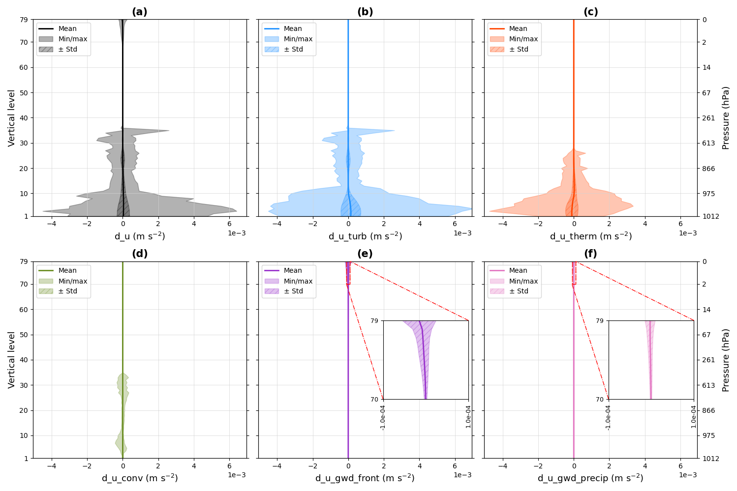
Figure 6 Mean vertical profile of the zonal wind tendency d_u (a) of the point A, located in high latitudes, with minimum/maximum envelope and standard deviation bounds (hatched areas). The data used are from a full-year simulation. The same types of curves as the zonal wind tendency can be generated for the physical processes involved in the decomposition of this tendency: turbulence (b), thermals (c), convection (d), gravity wave drag due to emission by fronts (e) and gravity wave drag due to emission by convective systems (f).

Figure 7 Same as Fig. 6 but for point B located in the subtropics.

Figure 8 Same as Fig. 6 but for point C located near the equator.

Knowing how turbulence is parameterized in phyLMDZ, it is possible to introduce physical knowledge into the learning process in an attempt to improve the performance of the emulator in terms of its representation of turbulence. In phyLMDZ, the zonal wind tendency due to turbulence is of the form:

$$\begin{array}{}\text{(13)}& m_z{\displaystyle \frac{\partial \mathit{u}}{\partial t}}=-{\displaystyle \frac{\partial }{\partial z}}{m}_z{\mathit{\varphi }}_u\end{array}$$

with m_z a mass-weighting coefficient depending on the altitude z and ϕ_u the vertical turbulent flux of the zonal wind which is given by:

$$\begin{array}{}\text{(14)}& {\mathit{\varphi }}_u=-K_z{\displaystyle \frac{\partial \mathit{u}}{\partial z}}\end{array}$$

where K_z is the turbulent mixing coefficient which depends on the altitude z. We introduce the laplacian of the zonal wind, noted Δu_z, which can be written as follows:

$$\begin{array}{}\text{(15)}& \mathrm{\Delta }{\mathit{u}}_z={\displaystyle \frac{{\partial }^{\mathrm{2}}\mathit{u}}{\partial z^{\mathrm{2}}}}.\end{array}$$

Turbulence can then be expressed in terms of this laplacian, up to a factor. With this in mind, we decided to add this vertical laplacian into the emulator as a predictor. The phyLMDZ model uses a hybrid pressure-based coordinate. Therefore, the thickness (in m) and mass content (in kg m⁻²) of each model layer vary with model level. Both affect the precise expression of the tendencies due to turbulence. For the zonal velocity at the level l, this expression is of the form:

$$\begin{array}{}\text{(16)}& {\displaystyle \frac{\partial {\mathit{u}}_l}{\partial t}}=K_l^{+}({\mathit{u}}_{l+\mathrm{1}}-{\mathit{u}}_l)-K_l^{-}({\mathit{u}}_l-{\mathit{u}}_{l-\mathrm{1}})\end{array}$$

where the coefficients $K_l^{+}$ and $K_l^{-}$ incorporate the turbulent diffusivities K_z computed above and below level l, the mass content of layers and their thickness. In order to reveal latent structural information without exposing too many details of the underlying parameterization, we use the above formula with $K_l^{+}=K_l^{-}=\mathrm{1}$ s⁻¹, i.e. a simple discrete three-point laplacian Δu_l, as additional input. This vertical laplacian is directly inferred from the zonal wind, hence we can refer to this variable as a hidden variable, often called latent variable. By applying Dirichlet boundary condition, we assume that for the first and last vertical levels, we have Δu₁=0 and Δu₇₉=0 respectively. The same equations (Eqs. 13–16) can be applied to the other five state variables v, T, qx1, qx2 and qx3, to obtain their vertical laplacians, respectively noted Δv, ΔT, Δqx1, Δqx2 and Δqx3. Then, we develop new emulators in which these laplacians were added as new predictors in order to improve the emulation of the turbulence. In the rest of the article, these emulators are referred to as laplacian-aware emulators. In this way, the new input stacked vector X has a length of 1030 and looks like:

$$\begin{array}{rl}\mathit{X}& =[\mathit{u},\mathrm{\Delta }\mathit{u},\mathit{v},\mathrm{\Delta }\mathit{v},\mathit{T},\mathrm{\Delta }\mathit{T},\mathit{q}\mathit{x}\mathit{1},\mathrm{\Delta }\mathit{q}\mathit{x}\mathit{1},\mathit{q}\mathit{x}\mathit{2},\\ & \mathrm{\Delta }\mathit{q}\mathit{x}\mathit{2},\mathit{q}\mathit{x}\mathit{3},\mathrm{\Delta }\mathit{q}\mathit{x}\mathit{3},\mathit{r}\mathit{o}\mathit{t},\mathit{sza},\mathit{psol},\mathit{SST}].\end{array}$$

The same pre-processing steps described in Sect. 2.3 are applied to this new input stacked vector X. The complexity of this new learning problem has been increased compared to the original problem due to the fact that we add six new predictors, each of which extends over the 79 vertical levels of the atmospheric column.

5.2 Training with physical knowledge

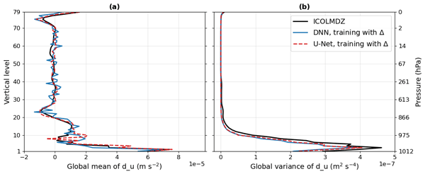
In order to assess the impact of adding new predictors, we first studied the global vertical profiles of the mean and variance (Fig. 9a and b) to compare them with the results obtained without the addition of these latent variables (Fig. 3a and b). As we can see in Figs. 3a and 9a, by comparing the same model architecture without and with the addition of laplacians, the global means of the predicted zonal wind tendency are quite similar in the vertical levels above 25. When we add the new predictors, the results are better in the first vertical levels, for both architectures. Moreover, we note that the predicted global mean profile is smoother for the U-Net than the DNN. Figures 3b and 9b highlight the fact that the initial learning revealed the difficulty of the DNN architecture in correctly representing the variability, contrary to the U-Net architecture, in the low vertical levels. Despite the fact that the representation of the variance is not perfect, it drastically improves with the new emulations for levels below 10. No improvement in the variance between levels 10 and 30 can be seen.

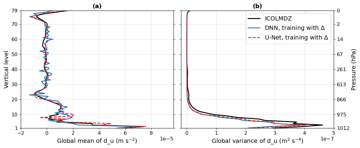
Figure 9 Global vertical profiles of the zonal wind tendency d_u of the mean (a) and the variance (b) for the test subset, obtained with the second training where physical knowledge is added. In these panels, the black curves represent the reference data from the ICOLMDZ simulation. The blue curves correspond to predictions made by the DNN while the dashed red curves represent the results obtained using the U-Net.

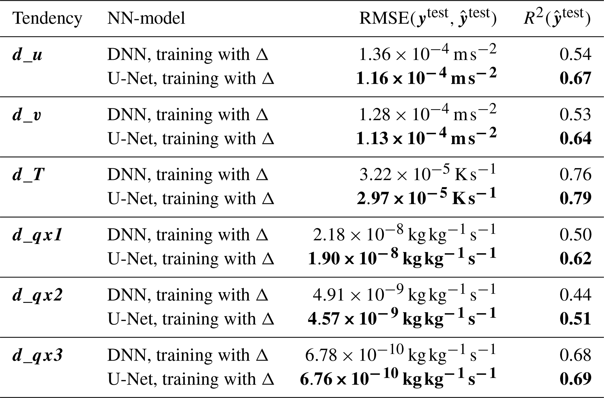
The global RMSE results for the zonal wind tendency obtained with the laplacian-aware emulators shown in Table 4 reveal that the U-Net architecture achieves a RMSE that is 14.7 % lower compared to the DNN. Thus, as with the emulators without laplacian (see Table 3), the U-Net model outperforms the DNN architecture when laplacians are added. Moreover, if we compare Tables 3 and 4 for a selected type of NN, the one in which laplacians have been added as predictors has a lower RMSE score. Indeed, the NN with laplacians has a global RMSE that is 8.1 % or 5.7 % – respectively for DNNs and U-Nets – better than that of the NN without laplacian. Thus, the addition of laplacians improves the prediction of the zonal wind tendency. When comparing the values of the coefficient of determination for the zonal wind tendency (see Tables 3 and 4), we underline that despite the laplacian, the DNN scores are lower than those of the U-Net without the laplacian. We see that the U-Net with laplacians (R²=0.67) outperforms the others, followed by the U-Net without laplacian (R²=0.63), then the DNN with laplacians (R²=0.54) and the last one is the DNN without laplacian (R²=0.46). Therefore, we improve the prediction of the zonal wind tendency by adding the laplacian of the zonal wind in both NN models. However, despite the addition of this new predictor, the DNN model does not achieve the performance of the U-Net in terms of predicting the zonal wind tendency.

Table 4 Results of the general metrics for the six tendencies over all time steps, cells and vertical levels of the test subset, to evaluate the two laplacian-aware emulators studied. The best metric values for each tendency are shown in bold.

Similarly to the emulators following the initial approach without laplacian, the zonal RMSE of the zonal wind tendency is calculated for the laplacian-aware emulators. The results are presented in Fig. 10a and b. As mentioned above for this metric in the context of the emulator without laplacian, the patterns in the first vertical levels are quite similar between the DNN and the U-Net, although the peak of the metric spreads at higher latitudes for the DNN. When comparing emulators where the laplacians have been added to emulators of the direct approach without them, we note that the new zonal RMSE is quite similar. The zonal RMSE differences of the zonal wind tendency between the original emulators and the new ones are shown in Fig. 10c and d. In either hemisphere, for vertical level below 10, the visible patterns between the latitudes 0 and 15°, but also between 30 and 90°, suggest that the laplacian-aware emulators are better in these regions. This improvement is even more significant for the DNN as the pattern is much more prominent than for the U-Net. For the other vertical levels, the gain from adding the laplacians is significantly smaller. In some regions, it seems that models without laplacian may even demonstrate better capabilities at higher altitudes, but this improvement is negligible compared to the enhancement observed at the lower vertical levels. Above the 10th vertical level, the zonal RMSE differences is mostly close to 0 meaning that the two models compared are similar: no improvement or degradation in the results is observed with the new emulators.

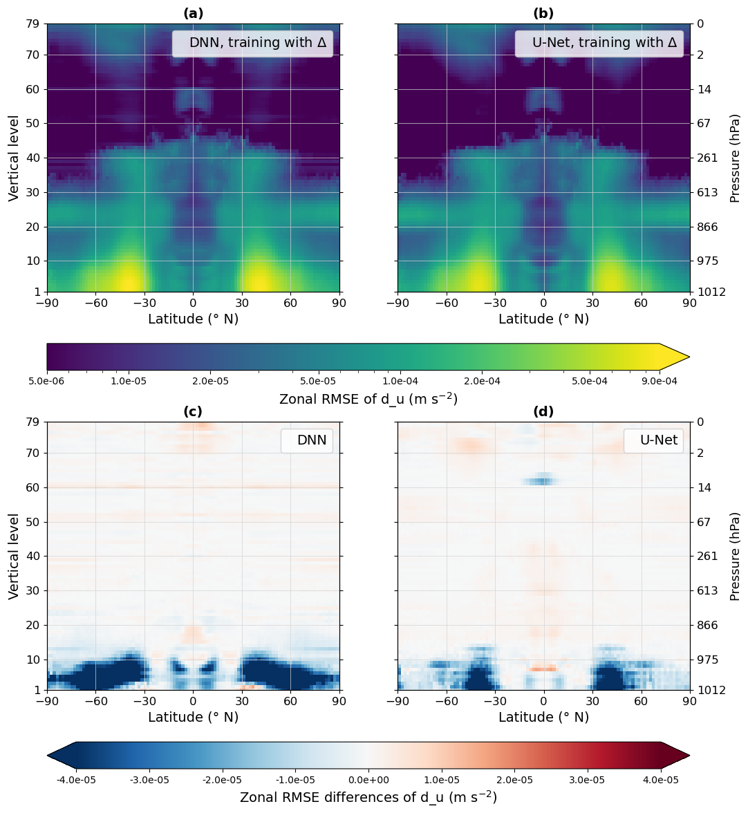
Figure 10 Cross-sections of the zonal RMSE of the zonal wind tendency d_u for the test subset, from the DNN (a) and from the U-Net (b) with laplacians. The colorbar displays data on a logarithmic scale. Panels (c) and (d) are respectively the zonal RMSE differences between DNN with laplacians (a) and DNN without them (Fig. 4a), and U-Net with laplacians (b) and U-Net without them (Fig. 4b). The blue colour indicates a better performance of the NN with laplacians, while the red colour corresponds to a better performance of the NN without laplacian.

5.3 Results for other tendencies

We examine the emulation of the other five tendencies with the laplacian-aware emulators. The laplacians of the six state variables have been added as predictors, motivated by the aim of improving the emulation of turbulence. Overall, for all the tendencies, we can draw the same conclusions as for the zonal wind tendency. Indeed, the global RMSE and the coefficient of determination R² shown in Table 4, and compared with those in Table 3, systematically indicate that laplacians help to obtain better predictions. We can highlight that, even if laplacians were added to the DNN model, it remains less efficient than the U-Net without these latent variables. However, this is not true for the ice water tracer tendency, noted d_qx3, for which the DNN architecture with laplacians is better than the U-Net without these predictors. Table 4 also shows that, overall, some tendencies are better predicted than others, such as the temperature tendency for instance. In the Supplement, the new global vertical profiles of these tendencies (Fig. S8a and b for d_v, Fig. S12a and b for d_T, Fig. S16a and b for d_qx1, Fig. S20a and b for d_qx2, Fig. S24a and b for d_qx3) are shown and can be compared with the profiles described previously in Sect. 4.3. It is also the case for the cross-sections of the zonal RMSE for each tendency (Fig. S9a and b for d_v, Fig. S13a and b for d_T, Fig. S17a and b for d_qx1, Fig. S21a and b for d_qx2, Fig. S25a and b for d_qx3). The results for the cross-sections of the zonal RMSE differences of the five tendencies (Fig. S9c and d for d_v, Fig. S13c and d for d_T, Fig. S17c and d for d_qx1, Fig. S21c and d for d_qx2, Fig. S25c and d for d_qx3) are also shown in the Supplement.

The global mean profiles of the tendencies are closely approaching those of the ICOLMDZ data with the laplacian-aware emulators, in both cases, although they are not perfectly identical to the reference data curves (see Figs. S8a, S12a, S16a, S20a and S24a). Moreover, for the vertical levels where the global mean is close to zero, the profiles still oscillate around the reference profile. As with the zonal wind tendency, the global variance profiles obtained with these new emulators remain underestimated, but they offer a better representation of the variability, especially in vertical levels where it is highest (see Figs. S8b, S12b, S16b, S20b and S24b). This is particularly noteworthy for the DNN model. For almost all the tendencies, the new predictive performance of the DNN is comparable to that of the U-Net. Nevertheless, we can identify some specific features depending on the tendency. For instance, the behaviour of the meridional wind tendency at the top of the atmospheric column has still not been captured by the emulators, in both cases. For the temperature tendency, the addition of laplacians does not seem to have any impact on the global variance for the U-Net: the DNN performs slightly better than the U-Net for certain vertical levels, thanks to the contribution of the laplacians. Concerning the results for the liquid water tracer tendency, the addition of the laplacians does not seem to have benefited the global mean. The curves are not smooth and still oscillate significantly around the reference global mean with large amplitudes. For the first levels, the profile from the DNN is significantly more underestimated compared to the first emulator without laplacian. However, the global variance highlights the improvement made by the DNN, particularly in the vertical levels with higher variability. Thus, for the liquid water tracer tendency, the improvement in global variance with the DNN seems to be at the cost of the global mean. For the ice water tracer tendency, the comparison shows that there has been no significant improvement. The curve of the DNN with laplacians even oscillates with larger amplitudes. However, the global mean curves from the predictions generally align with the behaviour of the global reference mean curve. At the variance peak, we observe a slight improvement in its representation by both models.

With the laplacian-aware emulators, we see the same patterns as with the initial approach, where the zonal RMSE is high, as shown in the cross-sections (see Figs. S9a and b, S13a and b, S17a and b, S21a and b and S25a and b). Nevertheless, these patterns seem less defined and spread for certain regions compared to initial learning, meaning that the addition of the laplacians has improved the prediction of these tendencies. This result is emphasized with the zonal RMSE differences (see Figs. S9c and d, S13c and d, S17c and d, S21c and d and S25c and d), for all the tendencies. With both NN architectures, the addition of physical knowledge into the learning process improves predictions whatever the tendency. Therefore, the same conclusions can be drawn as for the zonal wind tendency.

6 Results for a realistic setup

In this section, we present the results obtained for the emulation of the AMIP experiment. The study on the aquaplanet emulation allowed us to ensure that the emulators we developed reproduced the behaviour of the physics correctly and therefore to consider emulating a more realistic configuration where orography and continents are included. The same physical processes as for the aquaplanet experiment are used, but a larger diversity of situations needs to be represented. The integration of continental surfaces should certainly require a new structure for our datasets so that the variations in orography and the different types of surface can be taken into account by the emulators. However, for the sake of simplicity, we have applied the same methodology to sample data spatially and temporally as for the aquaplanet data. Figure S1 shows that cells used for the training process are distributed in such a way that they cover both oceanic and continental areas. We also used the same predictors as for the aquaplanet emulation. We trained four emulators – a DNN and a U-Net without laplacian and a DNN and a U-Net with laplacians – on the training dataset of the realistic configuration and monitored the learning process with the validation dataset for this same configuration.

Figure 11 shows the global vertical profiles of the zonal wind tendency of the mean and the variance for the test subset, obtained with the four emulators. The same conclusions as those obtained in the context of the aquaplanet configuration can be made. Emulators capture the global mean profile of the zonal wind tendency despite some difficulties encountered close to the surface. The variability represented by emulators is always underestimated particularly where it is the most pronounced, i.e., in the first vertical levels. The addition of latent variables, such as laplacians of the state variables, in the predictors provides a more controlled mean profile of the zonal wind tendency and contributes to improving the variability for the DNN but this is not the case for the U-Net architecture for which there is a degradation of the global variance profile. It would appear that this deterioration occurs in favor of the representation of the global mean profile. The U-Net with laplacians still remains the best model overall in terms of global RMSE for the zonal wind tendency. Indeed, this global RMSE is equal to $\mathrm{1.56}\times {\mathrm{10}}^{-\mathrm{4}}$ m s⁻² for the U-Net with laplacians, compared to $\mathrm{1.62}\times {\mathrm{10}}^{-\mathrm{4}}$ m s⁻² for the U-Net without laplacian, $\mathrm{1.76}\times {\mathrm{10}}^{-\mathrm{4}}$ m s⁻² for the DNN with laplacians and it reaches $\mathrm{1.96}\times {\mathrm{10}}^{-\mathrm{4}}$ m s⁻² for the DNN without laplacian. The addition of orography and continents can lead to significant differences in terms of the intensity of physical processes that are certainly linked to the spatially varying performances of the emulators in retrieving the mean and variance profiles of the zonal wind (not shown). With the addition of orography, the discrete approximation of the laplacian used as input may not represent as well the effect of turbulence on the zonal wind vertical structure. Further analyses need to be conducted to clearly understand this degradation.

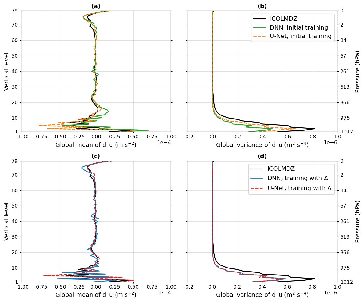
Figure 11 Global vertical profiles of the zonal wind tendency d_u of the mean (left) and the variance (right) for the test subset with the realistic configuration. Panels (a) and (b) show the results of the initial training, while panels (c) and (d) correspond to the second training where physical knowledge is added. In these panels, the black curves represent the reference data from the ICOLMDZ simulation. The green and blue curves correspond to predictions made by DNNs while the dashed orange and red curves represent the results obtained using U-Nets.

We have computed the global RMSE of the zonal wind tendency on all time steps and vertical levels for each emulator (Fig. 12). Regardless of the emulator studied, performances in terms of global RMSE are quite similar. For instance, the RMSE obtained over oceans is low, in particular between 30° S and 30° N, and it it also the case for some continental regions such as Africa. On the contrary, the RMSE is high for some continental regions for both emulators with and without laplacians. In particular, emulators from the initial training without the integration of physical knowledge show larger difficulties, notably for the DNN. These geographical regions with high RMSE values turn out to be mountainous areas, such as the Rocky Mountains in North America, the South of the Andes Mountains in Patagonia, the Himalayas and the Kamchatka peninsula in Russia. This suggests that the emulators are not trained on data where topography is heterogeneous. When we examine Fig. S1, we notice that the training dataset does not represent these rare areas. In this way, a few perspectives can be identified, they will be discussed briefly in Sect. 7.

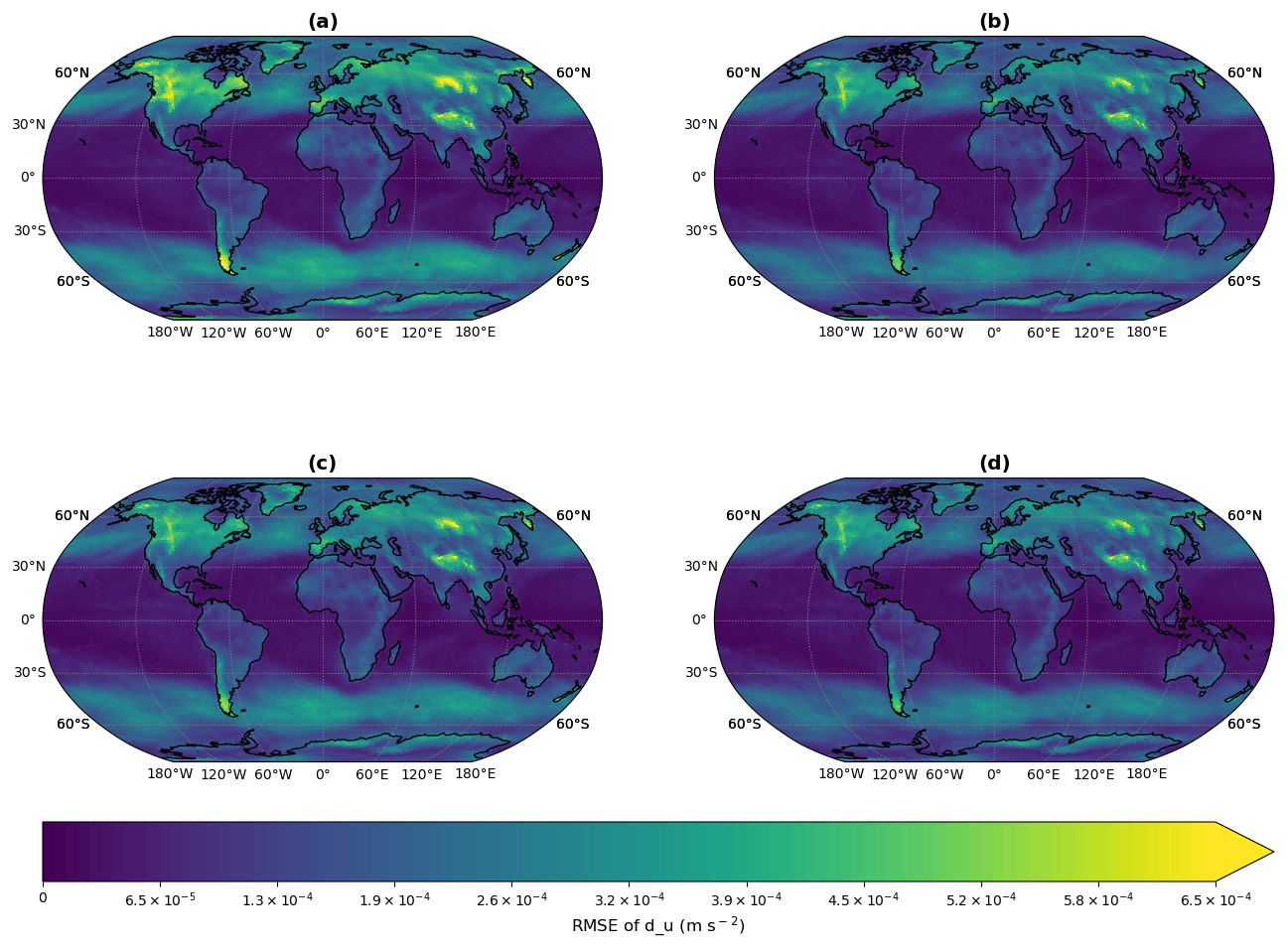
Figure 12 Maps of the global RMSE of the zonal wind tendency d_u for the test subset with the realistic configuration, calculated between data from ICOLMDZ and predictions made by an emulator. Panel (a) corresponds to the results from the DNN without laplacian, (b) those from the U-Net without laplacian, (c) those from the DNN with laplacians and (d) those from the U-Net with laplacians.

7 Conclusions and discussion

In this paper, we have explored the potential of emulating all the complex physical parameterizations of the ICOLMDZ atmospheric model, over the entire atmospheric column, in other words over the 79 vertical levels, and all grid points. To do so, we have developed several emulators based on different NN architectures and evaluated them in offline configuration. These emulators take the vertical profiles of state variables and variables relating to boundary conditions as input to reproduce the tendencies of state variables for each atmospheric column. The state variables are the zonal and meridional winds, the temperature, and the three water tracers. We have shown that a U-Net, where some ResBlock are added, is capable of reproducing the physical tendencies, while a DNN struggles to achieve as good results. After studying in more detail the physical processes involved in the tendencies studied, for the aquaplanet configuration, we demonstrate the effectiveness of adding some physical knowledge, in particular related to turbulence, into the learning process as predictors. Indeed, the addition of latent variables such as the laplacians of the state variables to the input of our emulators has improved the quality of the predictions in terms of variability. For instance, for the zonal wind tendency, this is particularly the case for the first ten vertical levels in the subtropics where the variability is higher. Moreover, this improvement is particularly significant for the DNN since, with the addition of these new predictors, this NN achieves global results comparable to the U-Net architecture. Nevertheless, even if this addition of new predictors primarily impacted the DNN, it should be noted that adding laplacians also improves the representation of the variance of the U-Net model, but to a lesser degree; its initial predictions (without laplacian) being better than those of the DNN.

Several hypotheses can be made about the better efficiency of the U-Net architecture compared to the DNN model. Firstly, the design of the U-Net favors the coherence and the dependence on the vertical structure. In theory, convolutional filters have the capacity to compute the laplacian and to use it for each vertical level. Moreover, the implementation of ResBlocks in the U-Net architecture helps to achieve better convergence by avoiding the vanishing gradient problem (Veit et al., 2016). Therefore, our study demonstrates the importance of integrating relevant physical predictors in NN models – here through the laplacian –, thereby reducing the black-box effect that exists with the use of DL models and improving interpretability.

In the context of the aquaplanet configuration, we have seen that the addition of laplacians has proven to be beneficial for all the tendencies, particularly in terms of variance. However, this enhancement varies in magnitude depending on the tendency studied. This reflects the influence of turbulence on the tendency. Even if turbulence appears in the breakdown of a tendency into physical processes, it is not specifically the main process, as in the case of the zonal wind tendency, for some regions. For instance, the physical processes contributing to the meridional wind tendency are the same as those for the zonal wind tendency. Most of the variability in the first vertical levels comes from turbulence, and the variability at the top of the atmosphere is due, in particular, to gravity wave drag from fronts. Concerning the temperature tendency, other physical processes are involved – for instance longwave radiation, evaporation and large-scale condensation – but turbulence is still present, especially at pressure levels below 261 hPa (corresponding to vertical levels below 40), without being the main process. This is also the case for the humidity tendency, as thermals and large-scale condensation, for instance, are two main physical processes involved in its calculation, in addition to turbulence which is present at pressure levels below 261 hPa. Thus, adding the laplacian to the predictors helps to improve the representation of turbulence for these tendencies. On the other hand, turbulence does not appear in the breakdown of the liquid water tracer and solid water tracer tendencies into physical processes. However, these two tendencies are strongly linked to the humidity tendency which depends on turbulence. This explains why the addition of laplacians does not result in a significant improvement of the variability for these two tendencies. As a result, the question of adding new variables that bring physical knowledge in the emulators to improve prediction of the other tendencies arises and should be considered.

The present work is a foundational first step towards a more ambitious project: emulating the physical parameterizations to make climate simulations and projections. To achieve this, several steps and major challenges remain.

We need to quantify the performance of each model in order to see if the contribution of ML accelerate the representation of physical parameterizations compared to phyLMDZ. For this, we estimate the time to obtain the six physical tendencies for one physics time step, on all cells across the globe and at all vertical levels, i.e. for one atmospheric column, with both the traditional parameterizations of phyLMDZ and the NNs, for the aquaplanet configuration. On the one hand, at the end of the simulation with ICOLMDZ, the dynamics part provides the total time spent in physics which amounts to approximately 4800 s for the whole year of simulation. Therefore, it takes an average of 0.140 s to obtain tendencies for a single physics time step. This diagnosis is obtained on Central Processing Units (CPUs) with a setup of 5 nodes and 164 physical cores used. On the other hand, the inference time estimation with our NNs is evaluated based on the predict() function from Keras/TensorFlow for a single physics time step. We estimate an inference time of around 0.045 s by time step with the DNN model, and we have a similar order of magnitude with the U-Net model, both models run on a single Graphics Processing Unit (GPU) NVIDIA V100. Therefore, in these configurations and for the inference of a single time step, the emulators offer a computational time gain of a factor of about three with respect to phyLMDZ. However, we would like to emphasize that estimating the gain when using an emulator instead of a physical model is much more complex. This is why these estimates should be considered as a preliminary test. It remains to be seen whether this gain would remain when the emulators are coupled with the dynamical core of the model, i.e., in an online setup. For instance, there is generally a substantial overhead when exchanging data from the dynamical core run on CPUs to the physics emulators run on GPUs. One way to alleviate this issue would also be to run the dynamical core on GPUs, which is already possible with the latest development of DYNAMICO.

A challenge is the generalisation to situations that have not been seen before. Emulators must be developed in such a way that they have the ability to cope with unseen climate conditions and generalise to different climates in a context of climate change. There have been recent developments (Clark et al., 2022; Beucler et al., 2024), to test the performance of the emulators on multi-climates to assess their ability to extrapolate and to obtain reliable and accurate results on scenarios that are not known by these emulators. For instance, Han et al. (2023) have created an emulator based on Convolutional Residual Neural Network to reproduce temperature and moisture tendencies, and cloud liquid and ice water from moist physics processes, with a realistic configuration. This study reveals the success to generalise, in an offline setup, to a warmer climate thanks to the use of a convective memory and a specific NN architecture.

After conducting the offline evaluation, the next step is to couple the emulator with DYNAMICO, the dynamics part of the model. This would allow us to assess the value of the learning process and study if the stability of the model is maintained. Even though the U-Net architecture outperforms the DNN during offline evaluation, it might not be the case when emulators are coupled with the dynamical core. That is why it would be interesting to assess the performance of both emulators. Moreover, the DNN might be faster than the U-Net since it has six times fewer parameters to optimize. The coupling between the climate model – written in Fortran and using CPUs – and the emulator – developed in Python and using GPUs – can be done in several ways thanks to software packages and interfaces (Curcic, 2019; Ott et al., 2020; Partee et al., 2021; Zhang et al., 2025). This online step is crucial to provide a better assessment of the value of the learning process, while also enabling us to investigate both the accuracy and the stability of online runs with our emulator. One key challenge currently under active study is achieving stable simulations when integrating the emulator with the rest of the model. New studies have recently been published in which the emulation of parameterizations has been carried out on a realistic configuration and the emulator developed has been coupled to the atmospheric model (Han et al., 2023). With their NNs tested for different configurations to reproduce subgrid processes – specifically turbulence, convection and radiation –, Lin et al. (2024) highlighted potential correlations between the performance of offline and online emulators. They also showed that online stability does not necessarily work conjointly with online performance. Hu et al. (2025) have demonstrated that it is possible to couple their U-Net emulator, developed to emulate all the physical variables required when using real geography, with their dynamical core, thus obtaining a stable hybrid model. This was made achievable especially thanks to the incorporation of cloud microphysics constraints and also through the addition of large-scale forcings and convective memory.

Finally, with the goal of conducting climate simulations and projections, these different steps must be repeated on a configuration where orography or even continental surfaces are added, in other words on a realistic configuration. We have performed a few preliminary offline tests on this type of realistic configuration. As it is the case for the emulation of the aquaplanet, we have shown that the results are promising. However, two major perspectives are emerging and must be the subject of further detailed studies. First, a new data sampling must be tested to improve the representation of rare geographical zones such as mountainous areas. Secondly, given the increasing diversity of situations with this new setup, the question of adding new variables in the predictors arises and needs to be studied. For instance, we could consider adding new variables linked to topography and other types of surfaces to provide knowledge on physical processes. This should help and guide the emulators to a better representation of the physical tendencies.