TOAR-classifier v2: a data-driven classification tool for global air quality stations

Accurate characterization of station locations is crucial for reliable air quality assessments such as the Tropospheric Ozone Assessment Report (TOAR). While urban and rural areas are relatively well-defined, the boundaries and identity of suburban areas remain ambiguous, overlapping with both urban and rural zones and varying due to cultural and social factors. This study investigates a machine learning approach to classify 24 348 stations in the unique global TOAR database as urban, suburban, or rural. We tested two different approaches: unsupervised K-means clustering with three clusters, and an ensemble of supervised learning classifiers including random forest, CatBoost, and LightGBM. We integrate these classifiers into a robust voting model, leveraging their collective predictive power. To address the inherent ambiguity of suburban areas, we implement a grid-search adjusted threshold probability technique. Our models, trained on the TOAR station metadata, are evaluated on 1979 unseen data points. K-means clustering achieves 71.88 % and 87.67 % accuracy for urban and rural areas respectively, but only 15.84 % for suburban zones. The supervised classifiers surpass this performance, reaching over 84 % accuracy for urban and rural categories, and 66 %–72 % for suburban areas. The adjusted threshold technique significantly enhances overall model accuracy, particularly for suburban classification. The good separation of our model is confirmed through evaluation with NO_x and PM_2.5 concentration measurements, which were not included in the training data. Furthermore, manual inspection of 30 randomly selected sites with Google maps reveals that our method provides a better label for the station type than the labels that were reported by data providers and used in the model evaluation. The objective station classification proposed in this paper therefore provides a robust foundation for type-of-area-specific air quality assessments in TOAR and elsewhere.

1 Introduction

Ozone in the troposphere plays a crucial role in human and environmental health (Post et al., 2012; Griffiths et al., 2021). As a significant atmospheric pollutant and greenhouse gas, ozone profoundly impacts air quality and contributes to the dynamics of climate change (Madronich et al., 2023; Orru et al., 2013). Accurate ozone monitoring data is essential for shaping public health policies and ecological regulations. Modern data infrastructures can be used to provide atmospheric scientists with the necessary metrics to quantify ozone's impact on climate, human health, and vegetation (Gaudel et al., 2018; Fleming et al., 2018; Mills et al., 2018; Teakles et al., 2017; Cooper et al., 2014; Monks et al., 2015; Schultz et al., 2015). In 2021, the International Global Atmospheric Chemistry project (IGAC) launched the second phase of the Tropospheric Ozone Assessment Report (TOAR-II) to undertake a comprehensive review of the global distribution and trends of tropospheric ozone. A key accomplishment of TOAR-II is the development of a new terabyte-scale relational database of surface ozone observations and related variables. This database includes hourly measurement data and enriched metadata from 1970 to 2023, collating information from over 20 000 measurement sites worldwide through collaboration among multiple data centers and individual researchers (https://igacproject.org/activities/TOAR/TOAR-II, last access: 24 June 2026). The new TOAR-II database replaces and extends the first TOAR database that has been described in Schultz et al. (2017a). Ozone levels exhibit significant regional variations and distinct patterns across different pollution environments. For example, urban environments with large ozone precursor emissions can exhibit “zero ozone” (i.e., ozone at sub-nmol fractions) situations and very large variability, while concentrations in rural areas tend to be smoother (Zhou et al., 2022; Schultz et al., 2017b). To accurately assess the ozone situation at individual locations and interpret ozone trends across the globe, it is therefore important to characterize measurement sites in a globally consistent and objective manner. While many measurement networks provide information about the station location or “type of station” and “type of station area”, this metadata information is inconsistent between regions and error-prone as it involves some subjective judgement (cf., Tapia et al., 2016).

In the first assessment of TOAR (Schultz et al., 2017a) pioneered a new way to classify stations in a globally uniform way based on a set of Earth Observation (EO) datasets that have been processed at the station locations. This method used manually selected threshold values of station altitude, population density, nighttime light intensity, NO₂ column density, and NO_x emissions to characterize stations as urban or rural. While this approach provided a useful distinction between “clearly urban” and “clearly rural” sites, it fell short of classifying all sites as almost half of the stations remained unclassified, see Fig. 1. Furthermore, the method was criticized for lack of an objective definition of the threshold values. Especially, the boundaries and characteristics of suburban areas remain ambiguous. Suburban zones, typically located at the periphery of cities and noted for lower density and residential land use, often overlap with both urban and rural regions. Their definition is shaped by cultural, social, and psychological factors, resulting in varied interpretations and a lack of universal consensus (Hesse and Siedentop, 2018; Airgood-Obrycki and Rieger, 2019). This emphasizes the need for an objective and automated station classification method. In this study, we propose a new machine learning (ML) approach to develop a more advanced and unbiased classifier using similar objective metadata from the TOAR-II database. Our primary objective is to create a machine learning model that classifies stations in the TOAR database as urban, suburban, or rural. We implement and compare two methodologies: unsupervised learning using K-means clustering, and supervised learning classifiers such as random forest, CatBoosting, and LightGBM. In supervised learning, a subset of station characteristics is known and used to train the classifiers which are then used to predict the class of unlabeled stations. The supervised models are evaluated individually and after applying a robust voting method. Furthermore, an adjusted threshold technique is applied to enhance the identification of suburban stations. The remainder of this paper is organized as follows: Sect. 2 describes the data and methods used, Sect. 3 presents the results and discussion, and a general conclusion wraps up the paper.

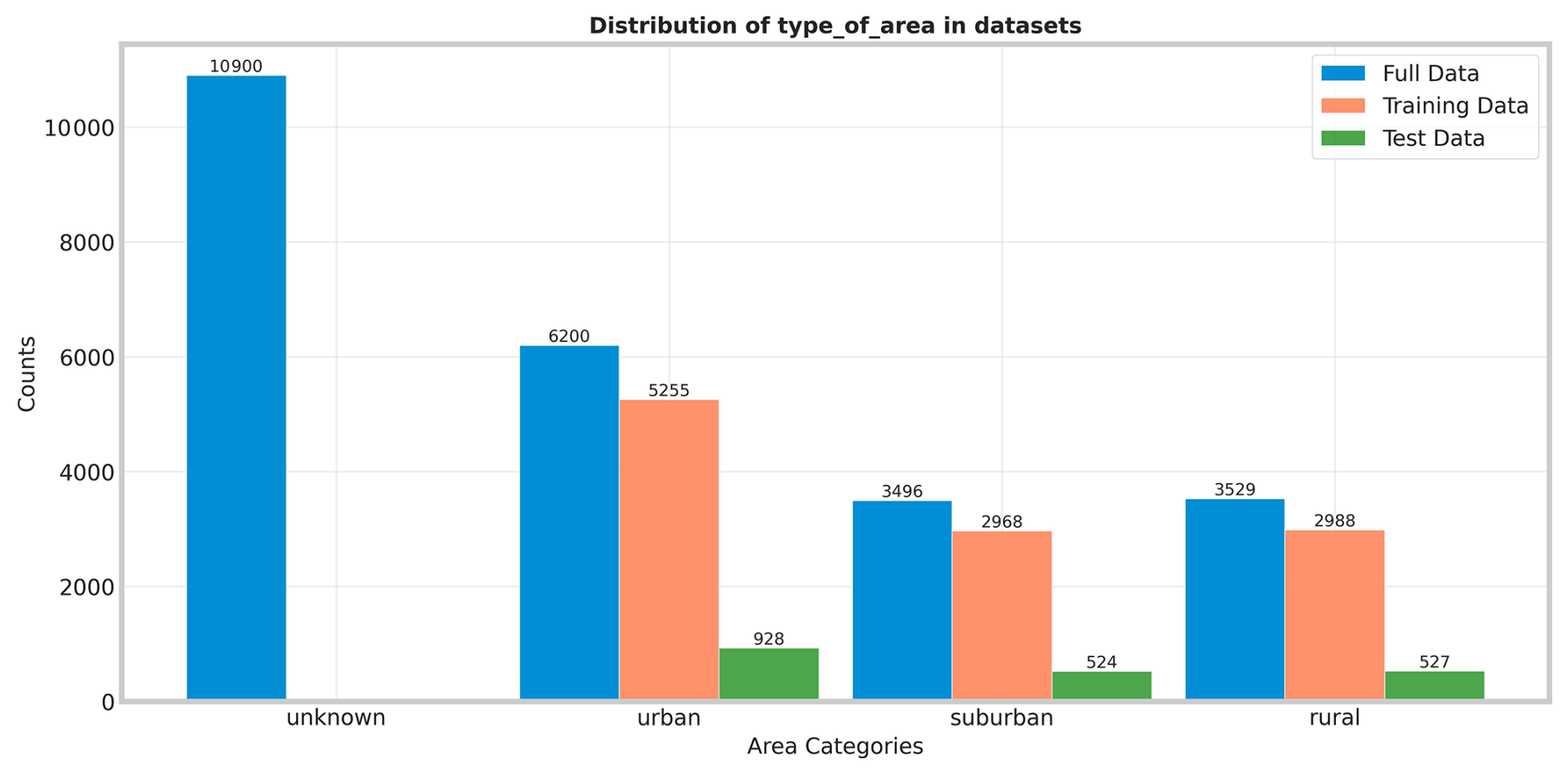
Figure 1 Distribution of unlabeled, training, and test data used for the supervised ML models as described in the text.

2 Data and methods

This section provides an overview of our data sources, machine methods used, and evaluation metrics. We begin by introducing the TOAR-II database and the station metadata that are used as inputs of the ML models. We then detail our data preparation process, including preprocessing, feature engineering, and feature selection, all critical steps in preparing data for ML models. Finally, we present a concise summary of the ML models employed in this study and the evaluation metrics used to assess their performance.

2.1 TOAR-II database and station metadata

Developed in the context of TOAR phase II, the TOAR-II database stands as one of the world's largest collections of near-surface ozone measurements and related information. The database can be accessed through web services which provide a comprehensive suite of ozone-related data products including standard statistics, health and vegetation impact metrics, and trend information (https://toar-data.fz-juelich.de/, last access: 24 June 2026). The TOAR-II database includes extensive information describing the locations of air quality measurement stations based on pollution-relevant properties. These properties are extracted from EO data and stored as station metadata in the database. This metadata offers contextual information about the measurement site, enabling station location characterization. Table 1 below summarizes all metadata used in this study including references to the data origin.

(Jarvis et al., 2008)(Jarvis et al., 2008)(Harris and Jones, 2017)(Kroehl, 1982)(Florczyk et al., 2019)(Granier et al., 2019)

Table 1 Station metadata in the TOAR database used in this work.

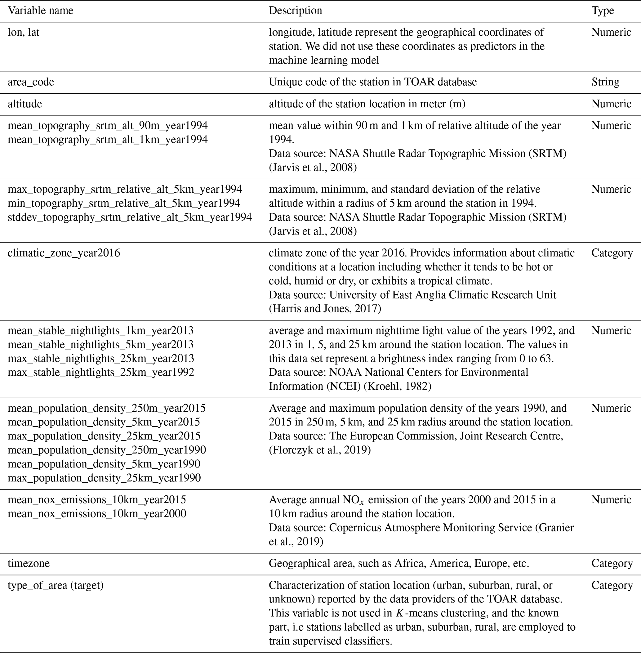
Some metadata, such as station coordinates, are provided by many air quality agencies and scientific institutions that contribute to the TOAR database. The other metadata elements listed in Table 1 stem from EO datasets, which were downloaded from the respective provider sites. A special web service called Geospatial point extraction and aggregation service (GeoPEAS) has been developed to compute the aggregate information from the original gridded products. More information about the EO datasets used in GeoPEAS can be found on https://toar-data.fz-juelich.de/api/v2/#stationmeta (last access: 24 June 2026). After the metadata extraction with GeoPEAS, all metadata are available as lists of key-value pairs with the keys corresponding to the variable names in Table 1. For further processing, this data was collected into one table with the keys as data columns and the individual stations as rows.

2.2 Data preprocessing and feature selection

The first step in our data preprocessing pipeline consists of cleaning the dataset. This involves removing all duplicate data points, replacing values of −999.0 with NaN to denote missing values, and eliminating rows where all metadata information is missing. To ensure consistency, we filtered out rows with inconsistent values, such as negative population density or negative maximum stable lights. In total, this step eliminates 211 stations out of 24 348 stations. For handling missing altitude data, we fill these with mean_topography_srtm_alt_90m_year1994. Other numerical missing values are estimated using the regression iterative imputer (Rubinsteyn and Feldman, 2016), and categorical missing values fill with most frequent instance. Categorical variables are encoded using OneHotEncoder from scikit-learn (Pedregosa et al., 2011b).

For K-means clustering, numerical features were scaled using standard scaling, and outliers were handled with IQR-based clipping within the range [Q1 − 1.5 ⋅ IQR, Q3 + 1.5 ⋅ IQR], where IQR (Interquartile Range) is the difference between the third quartile (Q3) and the first quartile (Q1). These preprocessing steps are essential to mitigate the algorithm's sensitivity to feature scale and outliers. For supervised learning algorithms, we applied a robust scaler (Pedregosa et al., 2011b) to the entire dataset, which proved more effective for this task compared to alternative scaling methods such as standard or min-max scaling. This scaling approach helps mitigate the impact of outliers and ensures consistent feature ranges. In the feature selection process, we prioritized variables containing the most recent available information, ensuring our model utilizes the most up-to-date data for classification. Notably, geographical coordinates (longitude-latitude) and station codes are excluded from the machine learning models to prevent overfitting to geolocation. Following preprocessing steps, the final dataset comprises 24 125 stations. Of these, 13 225 are labeled as urban, suburban, or rural, while the remaining 10 900 are unlabeled. The distribution of the processed data is presented in Fig. 1.

For the K-means clustering analysis, we allocated 22 111 samples for model training and reserved 15 % of the labeled data (1979 samples) for testing. The supervised models were trained on a smaller subset because only 13 225 stations were explicitly classified as urban, suburban, or rural by the TOAR data providers. The remaining 10 900 stations lacked this specific classification, being reported as “unknown” or without a designated category. We used 85 % of the labeled data (11 211 samples) for training while the remaining 15 % is allocated for testing. The distribution of training and testing datasets is presented in Fig. 1. As shown, the training dataset is imbalanced, with a higher number of urban stations compared to suburban and rural ones. However, the class imbalance is not severe. We address it by applying the Synthetic Minority Oversampling Technique (SMOTE) (Chawla et al., 2002) to the training data before fitting the supervised classifiers. It is important to note that SMOTE was applied exclusively to the training set and not to the test data. The trained classifier is then used to predict the characteristics of unlabeled stations as illustrated in Fig. 2.

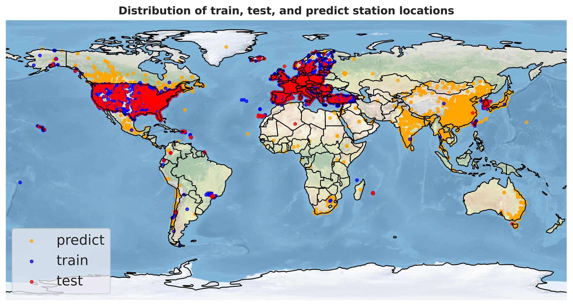
Figure 2 Distribution of unlabeled, training, and test data used for the supervised ML models as described in the text.

To ensure the reliability of our machine learning approach, we manually selected 35 stations with clear decision boundaries – that is, stations that are easy to classify as urban, suburban or rural, and excluded them from the training dataset. These stations were explicitly reported by data providers as urban, suburban, or rural, and we used Google Maps (Mehta et al., 2019) to manually verify and label them. During this process, we observed discrepancies between the labels provided by the data providers and those derived from our manual Google Maps analysis. Our models will first be evaluated on these 35 stations, with accuracy calculated both against the labels reported by the data providers and against the manually verified labels from Google Maps (referred to as hand-labeled data).

2.3 Machine learning algorithms and evaluation methods

This section is devoted to a concise overview of the machine learning techniques employed in this study. Additionally, we describe the evaluation metrics used to quantify the effectiveness and accuracy of our models.

2.3.1 Machine learning algorithms

• K-means clustering is a widely-used unsupervised machine learning technique that aims to partition data into k distinct groups called clusters (Bahmani et al., 2012; Sinaga and Yang, 2020; Pelleg and Moore, 2000). Each data point is assigned to the cluster with the nearest centroid. The algorithm seeks to minimize the within-cluster sum of squares, which measures the squared distances between data points and their respective centroids. One key requirement of K-means is specifying the number of clusters beforehand. We employed the heuristic elbow method to determine the appropriate number of clusters for our task. The elbow method is a heuristic technique used to determine the optimal number of clusters in K-means clustering. It works by plotting the within-cluster sum of squares (WCSS) as a function of the number of clusters and identifying the “elbow” point on the curve, which correspond to the optimal number of clusters (Ketchen and Shook, 1996). In our K-means clustering application, we determine that three clusters are optimal (see Fig. 3a), which aligns well with our objective of categorizing the stations into three groups: urban, suburban, and rural. However, it is important to note that visual inspection of correlation plots between individual metadata values Fig. 2 reveals rather fuzzy boundaries between clusters. This observation aligns with our expectations, given the diverse nature of urban, suburban, and rural locations across different countries, which can vary significantly in terms of industrial development, population density, and degree of urbanization in different countries (Zhang et al., 2024).

• Random Forest classifier is a widely-used machine learning algorithm for classification tasks. As an ensemble learning method, it constructs multiple decision trees through bagging during training and outputs the class that is predicted by the majority vote of the individual trees (Breiman, 2001). Known for its robustness, it naturally resists overfitting through random feature selection and typically requires minimal tuning compared to other algorithms. In our implementation, we train the Random Forest classifier with 500 estimators, employing entropy as the optimization criterion. These specific hyperparameters were determined through a grid search. We utilize the RandomForestClassifier from the scikit-learn library (Pedregosa et al., 2011a).

• The LightGBM (LGBM) classifier is a supervised machine learning algorithm that utilizes gradient boosting techniques and tree-based learning. It employs histogram-based algorithms and leaf-wise tree growth strategies, which contribute to accelerated training speeds and reduced memory consumption. LightGBM is particularly well-suited for handling large-scale datasets. Its lightweight architecture and optimized algorithm make it a popular choice for tasks requiring both speed and accuracy in prediction (Ke et al., 2017). In our implementation, we train LightGBM with 500 estimators using Python's open-source library “lightgbm” (Van Rossum, 2007).

• The CatBoost classifier is a machine learning algorithm that uses gradient boosting on decision trees, specifically designed to handle categorical features seamlessly (Prokhorenkova et al., 2018). CatBoost stands for “Categorical Boosting” and automatically handles categorical variables without requiring manual prepossessing. It uses symmetric trees and ordered boosting to prevent overfitting, and often outperforms other methods on datasets with categorical data. This makes it an attractive option for datasets containing both numerical and categorical variables. In our implementation, we employ the open-source CatBoost library and configure the model with 500 estimators to balance performance and computational efficiency.

• The Voting Classifier is an ensemble meta-estimator that combines predictions from multiple base models to enhance overall accuracy and robustness. It functions by either majority vote (“hard”) or averaging predicted probabilities (“soft”), effectively balancing the weaknesses of individual classifiers. This approach often yields superior generalization and reduced overfitting. Our implementation uses a soft voting strategy to aggregate predictions from a Random Forest, LightGBM, and CatBoost classifier via the scikit-learn library (Pedregosa et al., 2011a).

2.3.2 Leveraging Model Uncertainty to Enhance Suburban Classification Accuracy

Considering the inherent subjectivity in defining suburban areas, we refined our prediction methodology as follows: For any given station, if the model's highest probability for either urban or rural classification falls below a threshold, and if the second-highest probability corresponds to suburban classification, we interpret this as the model's uncertainty in categorizing the area between rural and suburban, or urban and suburban. In such cases, we classify the station as suburban. We applied the grid-search strategy in the range [0.35, 0.85] minimizing macro-F1, to find optimal threshold for each supervised algorithms. We obtain the thresholds of 0.5214, 0.4357, 0.5459, 0.4846 for random forest, CatBoost, LightGBM, and voting respectively. This approach acknowledges the model's indecision and leverages it to better capture the nuanced nature of suburban environments.

2.3.3 Evaluation

To evaluate our model's accuracy, we use a separate test dataset of 1979 samples, shown as red dots in Fig. 2. The test dataset consists of samples that were selected with stratification to ensure it reflects the distribution of real data, and intentionally excluded from both the training phase and the hyperparameter tuning process. This approach ensures that the evaluation metrics provide an unbiased assessment of the model's ability to generalize to new, unseen data, challenging the model in the real-world application scenario. We employed the following evaluation metrics to measure the performance of our machine learning model on this test dataset.

• Accuracy measures the ability of the machine learning model to accurately predict the outcome for the given input data. It is measured as the proportion of correct predictions to the total number of predictions made by the model, and given by the following formula:

  $$\mathrm{Accuracy}={\displaystyle \frac{\mathit{\#}\mathrm{Correct}\mathrm{Predictions}}{\mathit{\#}\mathrm{Total}\mathrm{Predictions}}}\times \mathrm{100}$$

  Here and in the following formulas, # stands for “Number of”.

• Per-class Precision: For a given class c, precision quantifies the fraction of correctly predicted instances of class c among all instances that the model predicted as class c:

  $$\begin{array}{rl}& \mathrm{Precision}\left(c\right)=\\ & {\displaystyle \frac{\mathit{\#}\mathrm{True}\mathrm{Positives}\left(c\right)}{\mathit{\#}\mathrm{True}\mathrm{Positives}\left(c\right)+\mathit{\#}\mathrm{False}\mathrm{Positives}\left(c\right)}}\times \mathrm{100}\end{array}$$

  Here, True Positives (TP) are the instances that actually belong to class c and were correctly predicted as such, while False Positives (FP) are the instances that do not belong to class c but were incorrectly predicted as instance of class c. Precision reflects how reliable predictions of class c are: high precision indicates that when the model predicts c, it is usually correct (Powers, 2020; Brodersen et al., 2010).

• Per-class Recall (Sensitivity, True Positive Rate): For a given class c, recall is defined as the proportion of true positive predictions for class c among all actual instances belonging to class c

  $$\begin{array}{rl}& \mathrm{Recall}\left(c\right)=\\ & {\displaystyle \frac{\mathit{\#}\mathrm{True}\mathrm{Positives}\left(c\right)}{\mathit{\#}\mathrm{True}\mathrm{Positives}\left(c\right)+\mathit{\#}\mathrm{False}\mathrm{Negatives}\left(c\right)}}\times \mathrm{100}\end{array}$$

  Here, False Negatives are the instances of class c that the model incorrectly assigned to another class. Recall characterizes the ability of the model to retrieve all relevant instances of class c; high recall indicates that the model rarely overlooks samples from this class (Powers, 2020).

• Per-class F1 Score: The F1 score for class c is defined as the harmonic mean of precision and recall:

  $$\mathrm{F}\mathrm{1}\left(c\right)={\displaystyle \frac{\mathrm{2}\cdot \mathrm{Precision}\left(c\right)\cdot \mathrm{Recall}\left(c\right)}{\mathrm{Precision}\left(c\right)+\mathrm{Recall}\left(c\right)}}\times \mathrm{100}$$

  This metric provides a single, balanced measure of a model's ability to achieve both high precision and high recall for class c, penalizing extreme values in either criterion. A high F1 score indicates that the classifier is effective both in accurately identifying instances of class c as well as capturing the majority of actual class c samples (Powers, 2020). (recall).

• Macro-F1: The macro-averaged F1 score is computed as the arithmetic mean of the per-class F1 scores, assigning equal weight to each class irrespective of its prevalence in the dataset:

  $$\text{Macro-F1}={\displaystyle \frac{\mathrm{1}}{N}}\sum _{c=\mathrm{1}}^N\mathrm{F}\mathrm{1}\left(c\right)\times \mathrm{100}$$

  where N denotes the total number of classes. This metric evaluates overall model performance by averaging across all classes and penalizes poor classification performance on minority classes, as each class contributes equally to the final score (Powers, 2020). Macro-F1 is widely used in multi-class classification evaluation for its insensitivity to class imbalance (Brodersen et al., 2010).

• Balanced Accuracy: Balanced accuracy is defined as the average of the per-class recall values:

  $$\mathrm{Balanced}\mathrm{Accuracy}={\displaystyle \frac{\mathrm{1}}{N}}\sum _{c=\mathrm{1}}^N\mathrm{Recall}\left(c\right)\times \mathrm{100}$$

  where N represents the total number of classes. Unlike standard accuracy, balanced accuracy accounts for class imbalance by assigning equal weight to each class regardless of sample frequency. This metric provides a more equitable evaluation in imbalanced classification scenarios, mitigating the bias introduced when a dominant class disproportionately influences the overall accuracy score (Brodersen et al., 2010; Sensoressa, 2025).

• Adjusted Rand Index (ARI) quantifies the similarity between the true cluster assignments and those predicted by the model. It operates by considering all possible pairs of samples and counting how many pairs are assigned to the same or different clusters in both the predicted and true clusters, (Chacón and Rastrojo, 2023; Chekir et al., 2017). The ARI score ranges from −1.0 to 1.0. A score approaching 1 indicates strong concordance between the true labels and the model's predictions, indicating that many sample pairs are clustered similarly in both clusters. A score near 0 suggests the clustering is comparable to random assignment. A negative score suggests that the predicted clusters frequently disagree with the true clusters, potentially performing worse than random assignment. This implies that sample pairs are often grouped differently in the predicted clusters compared to the true clusters.

• Normalized Mutual Information (NMI) measures the mutual information between the true clusters of the samples and the clusters assigned by K-means, normalized by the average entropy of the two label sets. It ranges from 0 to 1, where a score close to 1 indicates strong agreement between the true clusters and the K-means clusters. A score of 0 indicates no mutual information between clusters (Kvålseth, 2017).

To visualize the K-means clusters, we employed Principal Component Analysis (PCA), a dimensionality reduction technique that projects data onto orthogonal axes of maximum variance, enabling the representation of high-dimensional data in two or three dimensions (Abdi and Williams, 2010).

3 Results and discussion

In this section, we present and analyze the results of the various machine learning models applied to the TOAR station classification task. The first subsection details the outcomes of the unsupervised K-means clustering. The second subsection presents and analyzes the results from the three supervised methods. Finally, the last subsection discusses the overall performance and comparative insights of the different approaches.

3.1 Results for K-means clustering

Figure 2 shows the elbow plot, a heuristic technique used to determine the optimal number of clusters for K-means clustering. As the gradient of classification accuracy flattens at 3 to 4 clusters, these values for K represent the optimal choices. This result is very encouraging since we want to distinguish 3 different types of stations. As a first analysis of the K-means clustering, Fig. 3b shows the K-means predictions evaluated on 35 manually selected and labeled stations, with clear decision boundary from different categories for sanity check of our method. Table 2 presents the accuracy of K-means predictions on these manually labeled stations from the test set, comparing them with the characterization report from the TOAR database.

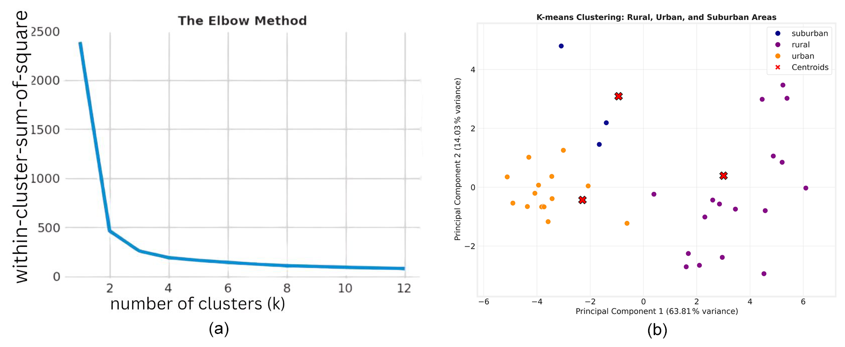
Figure 3 (a) Elbow method to determine the optimal number of clusters for K-means. (b) Different clusters for selected hand-labeled stations, the red points represent the centroid of different clusters.

Table 2 Global evaluation of K-means clustering: Accuracy, Balanced accuracy, ARI-score, and NMI-score on unseen test set labeled by the TOAR data providers, as well as on the 35 Manually selected with hand-labeled classifications.

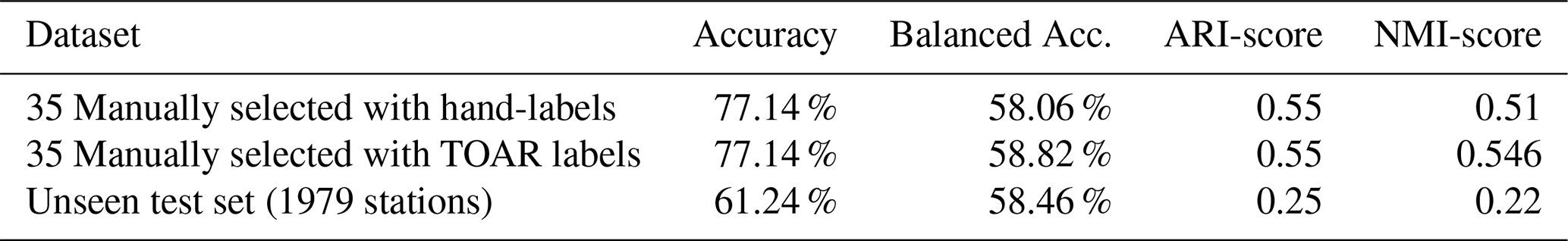
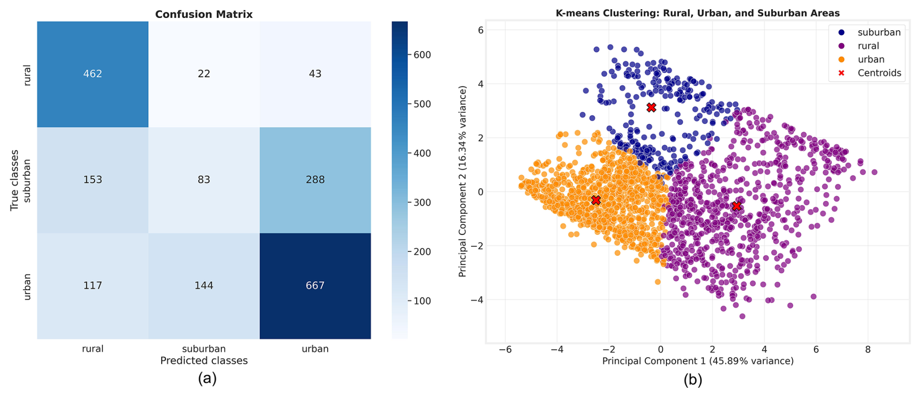
Figure 4 (a) Confusion matrix for K-means clustering, evaluated on 1979 unseen labelled by the TOAR data providers. (b) Cluster visualization of the previously unseen test data.

Figure 4a presents the confusion matrix computed from the K-means prediction and the classes from the TOAR database as ground truth, based on 1979 unseen test stations (see Sect. 2). This confusion matrix highlights the high accuracy of K-means in classifying urban and rural stations (87.67 % and 71.88 %, respectively, see Table 3, Recall's column). However, many instances exist where stations reported as urban or rural are classified as suburban, and vice versa. This misclassification is primarily due to the subjective nature of defining suburban areas, which often lie at the interface between rural and urban regions or exhibit a mix of urban-suburban or rural-suburban characteristics. Additionally, Fig. 4b visualizes the clusters defined by K-means for the 1979 unseen test stations. This visual representation clearly illustrates the fuzzy boundaries between the clusters and the noticeable spacing among the three centroids (depicted as red cross).

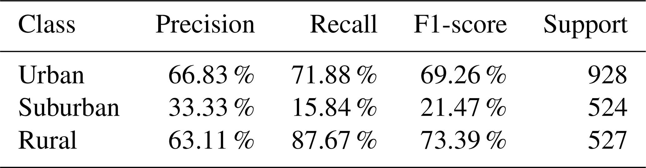
Table 3 Per-class evaluation of K-means clustering: Precision, recall, and F1-score on 1979 unseen test set labeled by the TOAR data providers.

3.2 Results for supervised classifiers

Here, we evaluate the results from the three supervised machine learning classifiers, Random Forest, LightGBM, and CatBoost. Furthermore, the results from the three models were subjected to a robust voting classifier to maximize the classification accuracy. We observed that the results of all algorithms are quite similar. The models demonstrated exceptional accuracy (> 83 %), high precision (> 85 %), and high F1-score (> 81 %) in predicting urban and rural areas. However, all models struggled with the suburban class, yielding accuracies slightly above 60 % (Table 5). As discussed above, the main reason for this lower accuracy can be attributed to the inherent subjective nature of defining this category. To address this issue, we implemented a strategy that capitalizes on model uncertainty. By adjusting the prediction probability threshold, as detailed in Sect. 2, we significantly enhanced the accuracy of suburban area classifications as shown in Table 7. Figure 5a presents the confusion matrix for the Random Forest classifier and Fig. 5b visualizes the feature importance. The global evaluation, i.e accuracy, balance accuracy, macro-F1 score, and weighted-F1 score of different classifiers are reported in Tables 4 and 6, which show the results before and after the probability threshold adjustment, respectively. While the overall accuracy remains relatively similar before and after the adjustment, the probability threshold adjustment significantly enhances the prediction accuracy for suburban stations, increasing it from a range of 60.85 %–65.72 % to 66.22 %–71.95 %, and also slightly increase the F1-score for the suburban, these can be seen in details in Tables 5 and 7 presenting the per-class evaluation before and after applying the probability threshold adjustment. We also note a slight drop in accuracy when classifying urban and rural stations. However, classification performance remains high across all classifiers, with accuracy values exceeding 80 %. Additionally, we conducted tests on our machine learning models using the manually labeled stations, similar to those used for K-means evaluation. In this test, we found that the classifiers predict the label report on TOAR by data provider for 35 manually selected stations with 100 % accuracy and achieve an 87.88 % accuracy for the manual classified stations.

Table 4 Global performance evaluation of models. Reported values are Accuracy, Balanced accuracy, Macro-F1 score, and Weighted-F1 score of random forest, LGBM, CatBoost, and voting classifiers before probability threshold adjustment, evaluated on 1979 test stations.

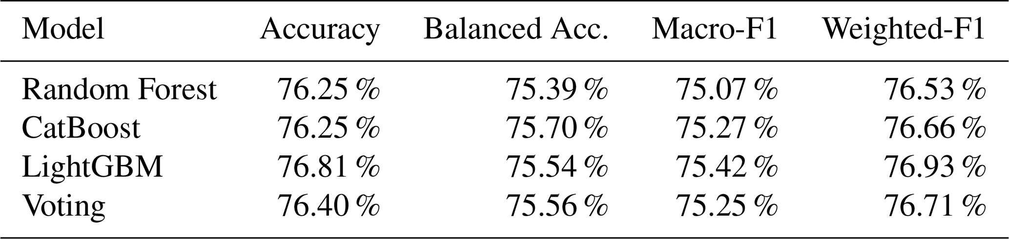
Table 5 Per-class performance evaluation of models. Reported values are Precision, Recall, and F1 score, of random forest, LGBM, CatBoost, and voting classifiers before probability threshold adjustment, evaluated on 1979 test stations.

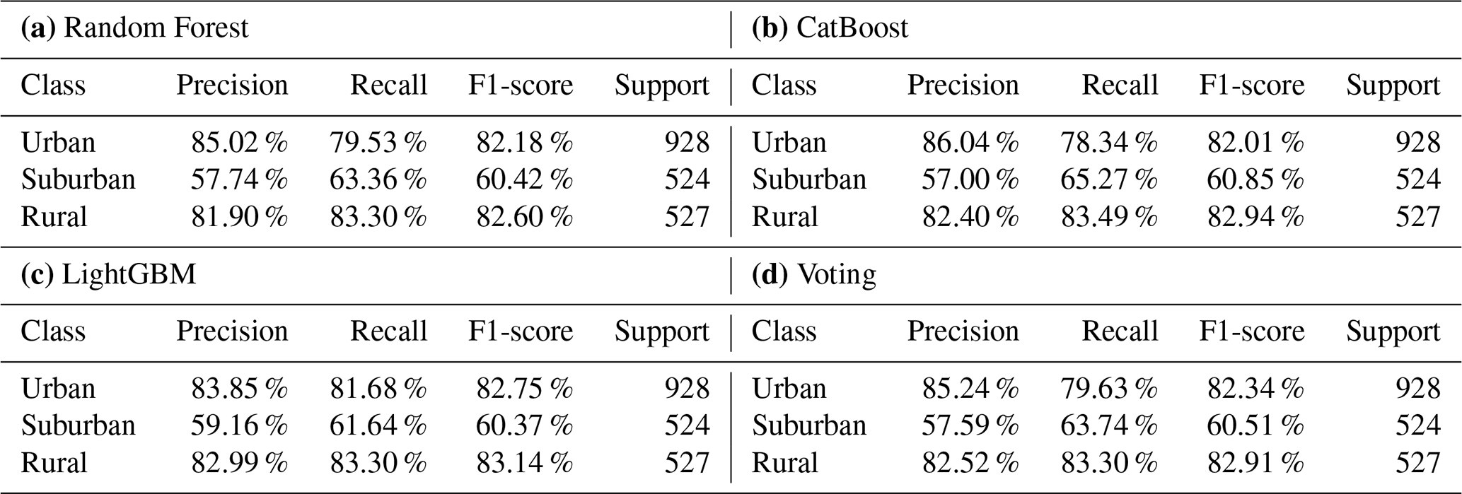
Table 6 Global performance evaluation of models. Reported values are Accuracy, Balanced accuracy, Macro-F1 score, and Weighted-F1 score of random forest, LGBM, CatBoost, and voting classifiers after applying probability threshold adjustment, evaluated on 1979 test stations.

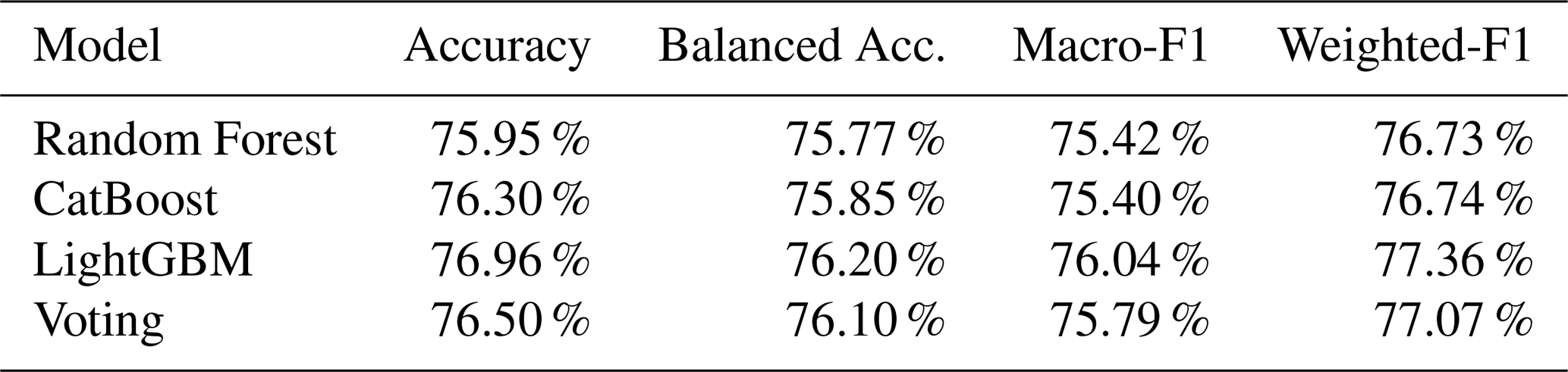
Table 7 Per-class performance evaluation of models. Reported values are Precision, Recall, and F1 score, of random forest, LGBM, CatBoost, and voting classifiers after applying probability threshold adjustment, evaluated on 1979 test stations.

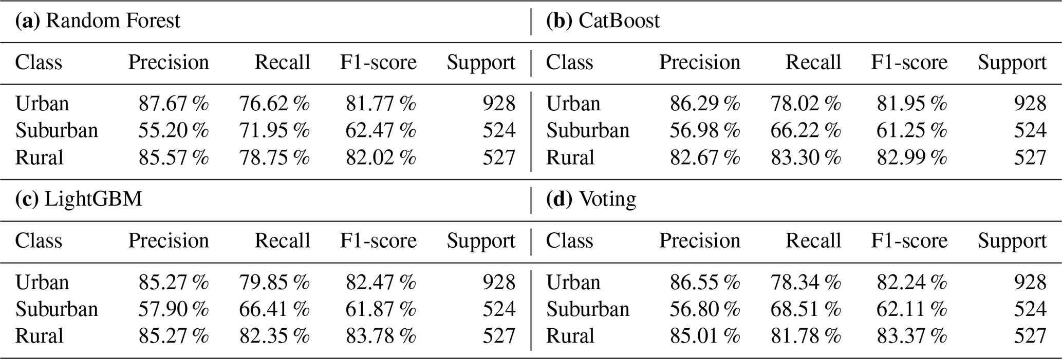
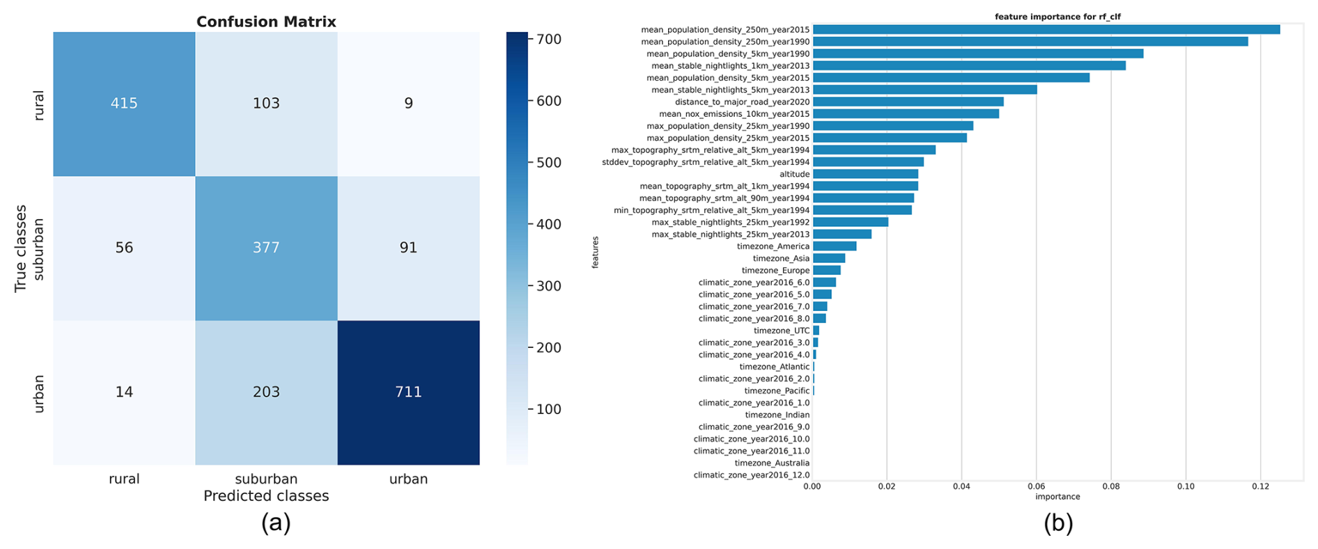
Figure 5 (a) Confusion matrix for random forest classifier, evaluated on 1979 test data points. (b) The feature importance for random, measuring the contribution of each variable in the classification process.

The implementation of the adjusted probability threshold yielded notable improvements in our classification model. While the enhancements for urban and rural station predictions were modest, the impact on suburban area classification was substantial. This is particularly significant given the inherent challenges in accurately identifying suburban zones. When compared to the unsupervised K-means clustering method, our supervised approaches demonstrated superior performance across all categories. The contrast was especially pronounced in the classification of suburban areas, where K-means exhibited a markedly low accuracy of just 15.84 %, low precision of 33.33 % and low F1-score of 21.47 %, see Table 3. In contrast, our supervised methods achieved significantly higher accuracy rates, higher precision, and higher F1-score underscoring their effectiveness in navigating the complexities of urban-suburban-rural distinctions.

3.3 Discussion

The supervised machine learning approach demonstrates remarkable performance, achieving prediction accuracies > 84 % for urban and rural stations when applied to previously unseen test data. This can already be used to accurately predict “urban” and “rural” labels. While the model's performance in identifying suburban areas initially showed slightly lower accuracy, this challenge was effectively addressed through the adjusted probability threshold.

Despite the promising results, the classification results are far from perfect. This can be partially attributed to inherent inaccuracies within the dataset itself. To investigate this issue, we conducted a detailed review and manual inspection of the 30 randomly selected misclassifications. For these stations, which are listed in Table 8, we visually inspected the areas around the stations on Google Maps (Mehta et al., 2019), using a zoom level of 11 or greater. While 6 of these cases revealed wrong classifications by our best ML model, the model's classification is actually more accurate than the label that was reported by the data providers in 16 cases. In the remaining 8 cases, neither the reported nor the ML model derived label was correct. In one of these cases, both the reported and ML based label was urban, while the station site is apparently located in a rural area. In the other case, visual inspection would place the station in the suburban class, while the reported category is urban and the ML model classifies the station as rural. However, for stations misclassified by our machine learning model, we observed ambiguous features that could misguide our model. For instance, surrounding neighborhoods of areas reported as urban but classified as rural by our model exhibited rural characteristics, such as lower population density (which is one of the important features used in the training dataset, see Fig. 5b) and more green space. This result, while initially counter-intuitive, can be explained by the strong robustness of tree-based ensemble methods to noisy datasets. Algorithms such as Random Forest, CatBoost, and LightGBM are specifically designed to mitigate the effects of noise and outliers through randomization and averaging techniques (Biau and Scornet, 2016). However, these 30 data points are insufficient to draw definitive conclusions.

Table 8 Closer analysis of some misclassified station locations.

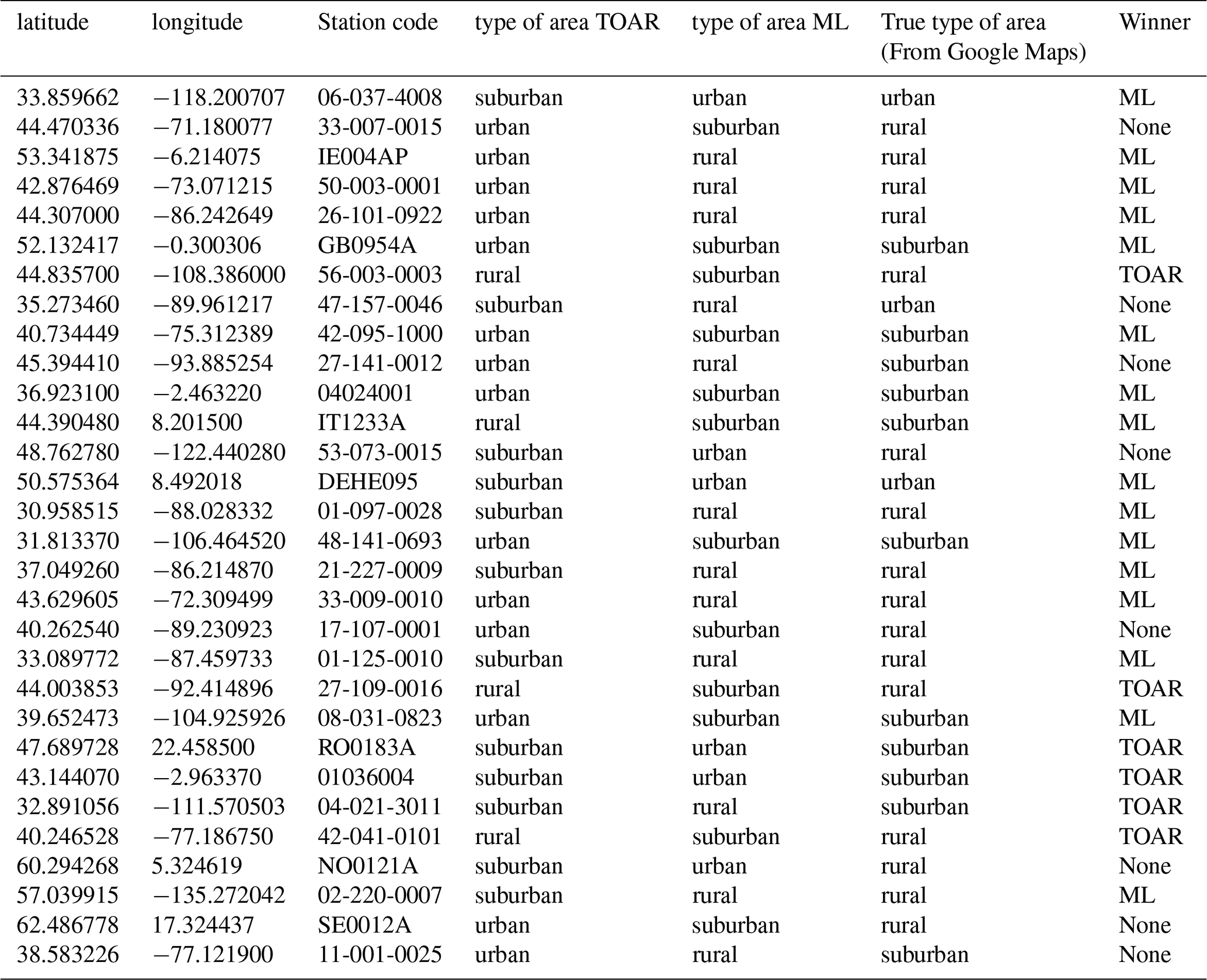
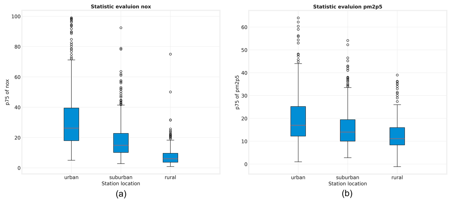
Figure 6 Evaluation of the supervised classification with independent data: (a) Box and whisker plot of the 75 percentile of the NO_x. (b) Box and whisker plot 75 percentile of the PM_2.5.

To further lend confidence to our results, we evaluated the 75-percentile statistics of the primary air pollutant concentrations NO_x and PM_2.5 from the TOAR database. We chose the 75th percentile, because urban areas typically exhibit fresh pollution with many high concentration events. This percentile captures such characteristics while being more robust than either the maximum value or a higher percentile. While data on these species is incomplete, there are sufficient measurements from several regions to yield a meaningful statistic. Figure 6 shows box and whisker plots of the 75-percentiles of NO_x and PM_2.5 concentrations aggregated for the year 2015 for the three classes. As expected, urban stations typically show substantially higher concentration levels compared to suburban sites, while rural stations show the lowest concentrations.

4 Conclusion

We investigated the use of machine learning models to objectively characterize station locations for global air quality data analysis. Specifically, we wanted to improve the station classification in the TOAR-I database that was described by Schultz et al. (2017a) and base it on an objective algorithm. As a side-effect we can now explicitly label stations as suburban that were falling between the urban and rural categories in the TOAR-I classification scheme. Our proposed models demonstrate excellent prediction capabilities for urban and rural areas. With the help of an adjusted probability threshold technique, we also obtain meaningful results on the suburban category, inasmuch this category can be described objectively at all. We noticed a limitation for evaluating the accuracy of our method due to obvious misclassification of stations in official databases. As discussed in (Schultz et al., 2017a), such errors can be introduced for various reasons. In some cases, we speculate that these misclassifications actually reflect true landcover changes (e.g., urban development), which have not been updated in the station metadata at the data providers' sites. Manual inspection of random test samples with disagreements revealed that the ML classifier was more often correct than the reported station type.

There is still room for improvement of the methods described here. On the one hand, a larger manual labelling effort using high-resolution EO data, could reduce the number of wrong target labels and reduce the noise in the training data. On the other hand, it may also be possible to employ modern ML methods with spatial context (e.g., Szwarcman et al., 2024) on such high-resolution EO data directly as a specialized land cover classification task. Nevertheless, the new TOAR station classifiers developed in this study provide a clear improvement over the previous method and can be employed in the TOAR-II ozone data analyses that will be reported in the forthcoming assessment papers.