runoutSIM v1.0: an R package for regionally simulating landslide runout and connectivity using random walks

Regional-scale runout modelling for landslide hazard assessment and land-use planning helps us understand not only the general likelihood of being impacted by their runout, but also how runout paths and distances vary under different environmental conditions. While R is widely used in geosciences for spatial prediction and susceptibility modelling, most existing runout models are not implemented directly in R, often requiring coupling with external software. This creates barriers for model development, modification, and integration with other geospatial and statistical tools.

To address this, runoutSIM is presented, an open-source R package for simulating the spatial extent, velocity, and connectivity of landslide runout at a regional scale. The model combines random walks to represent flow paths with a process-based approach to control runout distance and includes functionality to estimate the connectivity probability of runout from source areas intersecting with downslope features. In this model, the runout path and connectivity probabilities can also be adjusted by using spatial likelihoods of source cell predictions, such as those derived from statistical or machine learning models. In addition, runoutSIM provides an interactive map viewing environment within R that allows users to explore and query simulation results and related spatial data.

By implementing these algorithms natively in R, runoutSIM lowers technical barriers, supports flexible model development, and enables integration with data-driven approaches. We demonstrate the package in the Río Olivares basin, Chile, where a regional runout model optimized using a random grid search, machine-learning prediction of source areas, and simulation of runout connectivity help identify areas most susceptible to hazardous runout and potential source locations. runoutSIM provides a transparent and reproducible framework for regional runout modelling, supporting hazard assessment and enabling further development within R, a widely used geoscientific environment.

1 Introduction

Regional runout modelling for landslide hazard assessment and land-use planning allows us to understand not just the general likelihood of being impacted by runout, but also how the runout paths and distance may vary under different environmental conditions (Horton et al., 2024). These models are designed to work with data typically available at regional scales, making generalization and simplification essential features. While, hillslope-scale numerical models (Christen et al., 2010; McDougall, 2017; McDougall and Hungr, 2004) can provide more accurate insights for individual slopes or events, they rely on detailed geotechnical information that is rarely available at the scale needed for broad regional planning (Corominas et al., 2014). In contrast, regional runout analysis can help identify potentially hazardous hillslopes at large landscape scales to identify where more detailed geotechnical analysis can be applied to determine appropriate mitigation measures (Vagnon, 2020).

Similar to landslide susceptibility analysis, regional runout modelling can be applied to map general susceptibility to landslide runout, either through training on an inventory of past-events (Bornaetxea et al., 2025; Goetz et al., 2021; Horton et al., 2024; Lacelle et al., 2010; Mergili et al., 2019), or by simulating event-specific scenarios involving multiple landslides across large regions (Goetz et al., 2025; Wichmann, 2017; Wichmann and Becht, 2004). Unlike statistical or machine learning approaches used in regional susceptibility modelling, runout modelling helps bridge the gap between where slope failures are initiated and where their impacts may be felt – especially crucial for identifying hazards in flatter, downslope terrain (Lima et al., 2023). When coupled with data-driven approaches, such as using statistical or machine learning models to predict source areas, with process-based runout simulation, we can better capture regionally both the source and spatial extent of potential impacts (Goetz et al., 2021; Lima et al., 2023; Mergili et al., 2019). By integrating these techniques into a transparent, reproducible open-source workflow, we can ensure these geospatial tools are readily accessible not just to researchers, but to planners, consultants, students, and community stakeholders alike (e.g. D'Amboise et al., 2022; Mergili et al., 2015; Wichmann, 2017).

This paper presents an open-source geospatial R package, runoutSIM, for regional simulation of landslides, with the output including maps of their spatial extent, spatially varying velocity, and connectivity to other downslope features. The motivation behind developing runoutSIM in R is to provide a flexible, open-source, and cross-platform environment that integrates easily with advanced statistical, machine learning, and geospatial tools to facilitate the advancement of regional runout modelling. By providing this tool in R, one of the most widely used statistical and (geo)computing and visualization programming languages, runoutSIM aims to also simplify typical regional runout modelling workflows by consolidating analysis and map visualization within a single environment; common open-source regional runout modelling solutions require coupling with external software, such as R, to perform model calibration and validation (Goetz et al., 2021; Mergili et al., 2015; Wichmann, 2017).

2 Methods

2.1 Runout modelling with a random walk

The runoutSIM R package is designed to provide tools for regional runout simulation based on components of the Gravitational Process Path (GPP) model implemented in SAGA-GIS (Conrad et al., 2015) by Wichmann (2017). In runoutSIM, spatial modelling of runout extent is determined through a combination of random walks (Gamma, 2000), runout velocity equations (Perla et al., 1980), and Monte Carlo simulation applied to gridded DEMs. The individual flow paths from a source location are defined using a random walk process, where the likelihood of moving between neighboring grid cells is probabilistically determined, primarily based on slope steepness. To account for inherent uncertainty and variability in flow path prediction, which are mainly driven by slope variability, Monte Carlo simulations are employed to iteratively repeat random walks. By overlaying these repeated random walks, this iterative process captures a range of potential flow paths stemming from single or multiple source grid cells.

The random walk works by evaluating a 3×3 neighborhood window, starting from a source cell, prioritizing movement to downslope neighboring cells (Gamma, 2000). Transition probabilities, the probability of selecting the next downslope cell, are calculated based on slope, with probabilities weighted by the exponent of divergence to control the likelihood of selecting paths deviating from the steepest descent. A higher exponent of divergence distributes probabilities more evenly among candidate cells, increasing the chance of lateral spreading, while lower values favor steeper paths. Additionally, a persistence factor adjusts the transition probabilities by incorporating the influence of the previous flow direction, with higher persistence increasing the likelihood of continuity along the prior path. If any neighboring cells exceed a defined slope threshold, the steepest descent is automatically selected. In cases where multiple neighbors meet the threshold, ties are resolved using a random selection. The number of iterations (walks) determines the number of random walks performed from a source cell.

The termination or number of steps, and thus length, of each random walk path is controlled by the velocity computed for each state/grid cell using Perla et al.'s (1980) two-parameter friction model (PCM). The model follows a centre-of-mass approach, where movement is primarily governed by two parameters: (1) the sliding friction coefficient (μ) and (2) the mass-to-drag ratio ($M/D$). The velocity at a given grid cell (v₁, in m s⁻¹) is determined based on the velocity of the preceding cell (v_i−1), the local slope angle (θ, in degrees), the horizontal distance between cells (L_i, in m), gravitational acceleration (g, in m s⁻²), and the two friction-related parameters μ and $M/D$ (in m). The sliding friction coefficient (μ) can be provided as a global value or as spatially distributed values within a raster with the same extent and resolution as the input DEM. The resulting simulated runout extents are represented by cumulative traverse frequencies for each grid cell: the frequency with which individual grid cells are travelled through by a walk during the random walks.

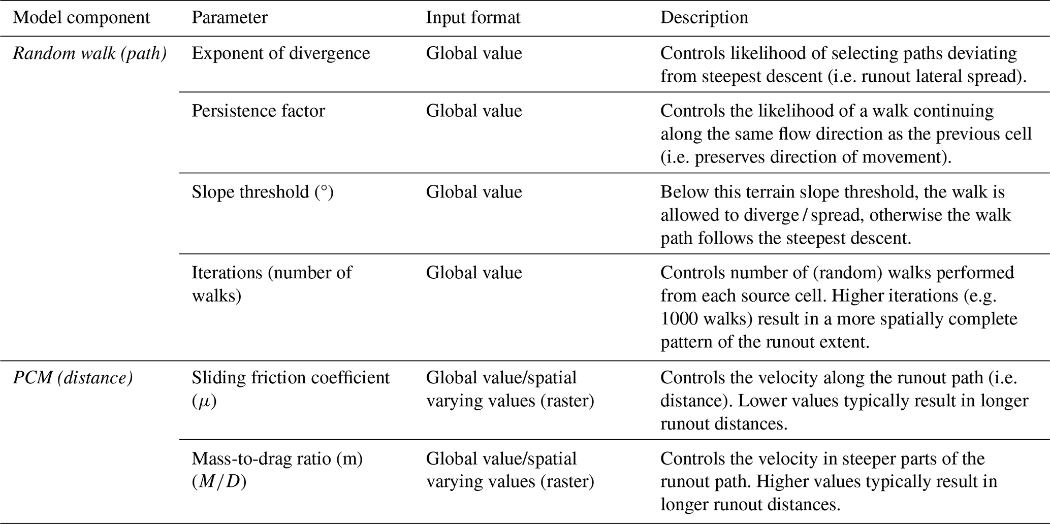
For more details on the random walk and PCM modelling components, its is recommended to refer to Wichmann (2017) and (Goetz et al., 2021) – an additionally short description of the random walk and PCM model parameters are provided in Table 1. The minimum input requirements for the random walk and PCM modelling components are a DEM, and location coordinates of source areas.

Table 1 Random walk and PCM parameters that control simulated runout path and distance.

In addition to re-creating the runout extent of observed events, the runoutSIM runout modelling framework is designed to integrate the spatial prediction of source areas with process-based runout simulation, using random walks for regional runout susceptibility modelling. The general concepts of the random walk and PCM modelling components, as well as their application for regional-scale runout modelling, optimization, and validation, are described in Goetz et al. (2021). The present study extends this work by implementing the entire framework in R and by introducing functionality to assess the connectivity, i.e., the likelihood of source areas impacting downslope features.

2.2 Mapping traverse frequencies, probabilities, velocity and connectivity

2.2.1 Traverse frequency

The frequency that a grid cell is traversed by random walk paths is referred to as the traverse frequency (Fig. 1a). Traverse frequency is simply the number of times an individual grid cell is visited across overlapping random walk iterations. This can either be starting from single or multiple source cells. In general, the spatial pattern of traverse frequencies can be interpreted as areas likely in the path of the simulated runout; however, a higher traverse frequency does not necessarily correspond to a higher likelihood of impact. In depositions areas, spread of the runout random walks is more likely to occur which results in overall lower traverse frequencies due to dispersion. Here, the open and less steep terrain can have a greater variation in walk paths. Therefore, traverse frequencies in the deposition zone may be interpreted as an approximation of the uncertainty a grid cell is traversed. Having higher dispersion, which results in lower transition frequencies, means it is harder to pinpoint the exact path of an individual runout event may follow (Fig. 1a vs. Fig. 1b).

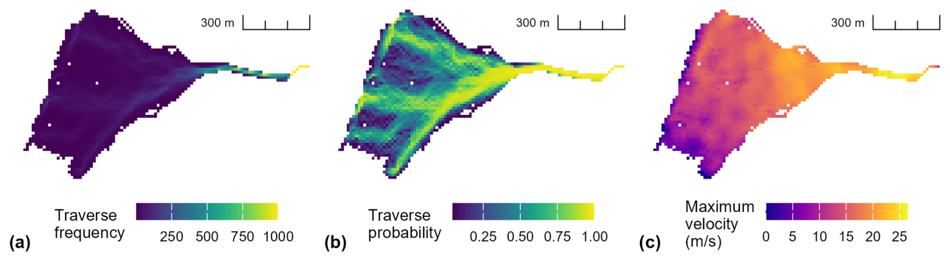
Figure 1 An example of traverse frequency (a), probability (b) and maximum velocity (c) simulated from a single source cell – runout travelling downslope right to left in each figure.

2.2.2 Traverse (spatial) probability

The probability that the simulated runout paths intersect with a given grid cell is referred to as the traverse probability (Fig. 1b). However, because traverse frequency values are often reduced in deposition areas, the traverse probability cannot be obtained by simply summing individual probabilities derived from transition frequencies divided by the number of walks in each source-cell simulation. Instead, similar to Mergili et al. (2015), who used a cumulative distribution function (CDF), an empirical cumulative distribution function (ECDF) to better represent the spatial likelihood or probability of runout following a certain downslope path. The ECDF is a non-parametric estimator of the CDF, resulting in this case with a spatial probability density surface that reflects how likely a runout path is to traverse a given cell, relative to all simulated paths and across all walks and source cells. It is important to emphasize that these probabilities are relative to the entire simulated area, and indicate the relative spatial likelihood of path traversal, not absolute probabilities.

2.2.3 Traverse velocity

For random walks from an individual source cell, the maximum traverse velocities for each grid cell can be mapped (Fig. 1c). For overlapping random walks from multiple source cells, these maximum velocities can be aggregated using a summary statistic of choice (e.g. maximum of maximum, or average maximum velocities). In the random walk framework, velocities estimated using the PCM model can be interpreted as an indicator of local flow mobility.

2.2.4 A random walk connectivity probability

A unique feature of this implementation of random walk runout modelling, is the ability to estimate the probability that a source grid cell will connect with a given feature of interest (e.g. river channels, road infrastructure or buildings) from the random walks – the connectivity probability. We determine the probability P_connect that a source grid cell (x_s) at location x connects with any of the feature grid cells (x_f) by analyzing the repeated random walks. Where, a feature of interest is represented by a set of grid cells $F=\mathit{\left\{}\right(x_{\mathrm{1}}),(x_{\mathrm{2}}),\mathrm{\dots },(x_{\mathrm{f}}\left)\mathit{\right\}}$, by converting polygon features to grid cells, and each walk is a sequence of grid cells $W_j=\mathit{\left\{}\right(x_{\mathrm{1}}),(x_{\mathrm{2}}),\mathrm{\dots },(x_j\left)\mathit{\right\}}$. This probability is calculated as the proportion of $N_{\left(x_{\mathrm{s}}\right)}$ walks that intersect with the feature F at least once:

$$\begin{array}{}\text{(1)}& P_{\text{connect},\left(x_{\mathrm{s}}\right)}={\displaystyle \frac{{\sum }_{j=\mathrm{1}}^{N_{\left(x_{\mathrm{s}}\right)}}{I}_{j,\left(x_{\mathrm{s}}\right)}}{N_{\left(x_{\mathrm{s}}\right)}}}\end{array}$$

where:

$$\begin{array}{}\text{(2)}& I_{j,\left(x_{\mathrm{s}}\right)}=\left\{\begin{array}{ll}\mathrm{1},& \text{if walk}j\text{intersects feature}F,\\ \mathrm{0},& \text{otherwise}.\end{array}\right.\end{array}$$

Here, $I_{j,\left(x_{\mathrm{s}}\right)}$ is an indicator function that evaluates whether walk j intersects the feature F. For each walk, it outputs 1 if there is at least one intersection and 0 otherwise. Summing the outputs of the indicator function across all walks from the source cell gives the total number of intersecting walks, which is then divided by the number of repeated walks $N_{\left(x_{\mathrm{s}}\right)}$ to calculate the proportion and thus probability of connectivity. Note in Eqs. (1) and (2) that the traverse frequencies/probabilities are not necessary for calculating the probability of connectivity.

This straightforward approach captures process behaviour while representing features in a grid-based format, enhancing computational efficiency. By relying on index comparisons rather than calculating actual intersections from vector data, the method reduces computational complexity.

2.3 Adjusting traverse frequencies, probabilities and connectivity probabilities

The spatial likelihood of a grid cell being classified as a source cell, often predicted from statistical or machine learning models, can be used to adjust the traverse frequencies (and ECDF probabilities) as well as the connectivity probabilities, $P_{\text{connect}\left(x_{\mathrm{s}}\right)}$. Such adjustment is important because not all grid cells have the same probability of generating landslides; weighting by source likelihood ensures that runout modelling reflects both the dynamics of path propagation and the spatial variability in initiation susceptibility. This adjustment is performed by multiplying the traverse frequencies for random walks simulated from an individual source cell, F_{traverse (x)}, by the spatial classification probability of that source cell, $P_{\text{source}\left(x_{\mathrm{s}}\right)}$, to obtain adjusted traverse frequencies, F_{traverse, adjusted (x)}. In other words, the traverse frequencies for each grid cell can be weighted by the source cell probability before aggregating the random walks from multiple source cells. This weighting is optional, but when spatial likelihood of initiation is available, it provides a more realistic representation of runout likelihood by accounting for variation in source susceptibility rather than assuming all potential source cells are equally likely to generate events.

$$\begin{array}{}\text{(3)}& F_{\text{traverse,\hspace{0.17em}adjusted}\left(x\right)}=F_{\text{traverse}\left(x\right)}\cdot P_{\text{source}\left(x_{\mathrm{s}}\right)}\end{array}$$

The connectivity probabilities can be adjusted using the source cell probabilities by multiplying the probabilities together.

$$\begin{array}{}\text{(4)}& P_{\text{connect,\hspace{0.17em}adjusted}\left(x_{\mathrm{s}}\right)}=P_{\text{connect}\left(x_{\mathrm{s}}\right)}\cdot P_{\text{source}\left(x_{\mathrm{s}}\right)}\end{array}$$

Note that adjusting the traverse frequency will not impact the connectivity probability since the connectivity probability is determined independently from the traverse frequencies, since it is based on an indicator function for runout path-feature intersections (Eqs. 1 and 2).

2.4 Implementation in R for geocomputing

runoutSIM compiles the approaches described above to perform runout simulation entirely within the R environment (R Core Team, 2025). A key motivation for re-implementing the random walk and PCM components, originally from the GPP model in SAGA-GIS, was to create a flexible sandbox within R. This allows algorithms to be modified or extended; for example, to estimate connectivity probabilities without needing to work across multiple software platforms or programming languages.

On the programming side, much of the development of this package has focused on ensuring computational efficiency of the random walk and PCM algorithms within R, as well as enabling their implementation within parallel processing frameworks to improve performance when simulating random walks from thousands of source cells. To handle the large datasets generated by walks and raster data in regional applications, the results of the runout walks are stored in sparse matrices, which index the frequency of a cell being traversed by individual cell IDs. This approach reduces memory usage and improves computational efficiency in R. Additionally, traverse frequencies from random walks corresponding to each individual source cell are stored separately, allowing for flexible approaches to aggregating overlapping runout paths.

Implementing the model in R also streamlines the integration of advanced statistical and machine learning techniques for predicting and validating source areas, and it opens the door for future extensions of runoutSIM. It supports parameter optimization through approaches such as random grid searches and exhaustive grid searches, making it easier for users to customize and develop the model further.

2.4.1 Package dependencies and RStudio interaction

runoutSIM depends on several R packages. The terra (Hijmans et al., 2025), and sf (Pebesma et al., 2025) packages are used for spatial (vector and raster) data handling. The leaflet (Cheng et al., 2024), leafem (Appelhans et al., 2025), and htmlwidgets (Vaidyanathan et al., 2023) packages are used to develop custom plotting functions in runoutSIM to create interactive spatial mapping of the runout simulation results (Fig. 2). When run in RStudio (Posit team, 2025), the multi-pane layout and implementation of leaflet for interactive mapping allows users to explore model results alongside basemaps, satellite imagery, and terrain data within a single environment. Users can interactively zoom, inspect polygon attributes, and query grid cell values, making it easier to compare simulation outputs to available reference data. This reduces the need to export results to an external desktop GIS, streamlining the development process of reviewing, interpreting, and refining model performance. The interactive maps can also be exported as an HTML document for collaborators or stakeholders, to explore in a specialized software-free environment (i.e. any desktop or mobile web browser).

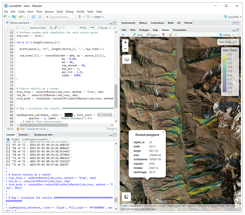
Figure 2 Example of the runoutSIM package workflow in RStudio (Posit team, 2025), where the runout simulation results can be visualized interactively through leaflet powered maps. Imagery sources: Esri, DigitalGlobe, GeoEye, i-cubed, USDA FSA, USGS, AEX, Getmapping, Aerogrid, IGN, IGP, swisstopo, and the GIS User Community – Powered by Esri.

3 Case study

3.1 Regional debris flow runout and connectivity modelling

This case study demonstrates the use of the runout model to regionally simulate the spatial likelihood of debris flows and to assess the connectivity of potential source areas to a main river channel and stream network. The modelling workflow involves (1) globally optimizing model parameters for regional application, (2) spatially predicting potential source areas using machine learning, and (3) simulating runout and connectivity from these sources. All steps are implemented within runoutSIM in the R environment.

3.2 Study area and data

The study area is the Río Olivares basin in the central semi-arid Chilean Andes, located ∼50 km east of Santiago. The basin spans 385 km², ranging in elevation from ∼1500 m at its southern outlet to ∼6000 m in the northeast. Situated in the Main Cordillera, the landscape is characterized by steep terrain formed primarily by Eocene–Miocene volcanic rocks (Sepúlveda et al., 2014). The main valley runs north–south, flanked by tributary valleys and prone to debris flows triggered by intense rainfall, earthquakes, or snowmelt (Sepúlveda et al., 2006).

The debris flow inventory is a dataset of 73 debris flow polygons manually mapped based on photo-interpretation of high spatial resolution (0.50 m) satellite imagery (2000–2019) from CNES/Airbus, Maxar Technologies, DigitalGlobe, GeoEye, i-cubed, USDA FSA, USGS, AEX, Getmapping, Aerogrid, IGN, IGP, swisstopo, and the GIS User Community from available Google Earth and Esri World Imagery basemaps (accessed June 2025). One source point for each runout polygon was also manually mapped near the highest point in elevation. These source points were used for runout model optimization. Since, no dates are tied to these events, we can only presume the regional runout model represents general debris flow susceptibility conditions. The DEM used is a free, publicly available ALOS PALSAR radiometrically terrain corrected high-resolution DEM with a spatial resolution of 12.5 m.

3.3 Regional runout parameter optimization

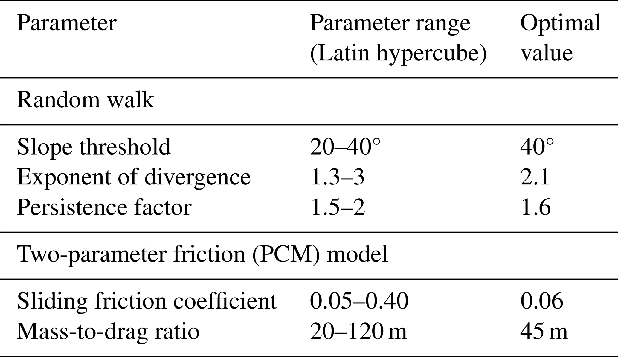
The parameters for describing the dispersion of the random walk and the two-parameter friction (PCM) model were calibrated using a random grid search based on 50 parameter sets drawn from a Latin hypercube sample (Table 2). Parameter ranges were defined for the slope threshold (20–40°), exponent of divergence (1.3–3.0), and persistence factor (1.5–2.0) of the random walk, as well as for the sliding friction coefficient (0.05–0.4) and the mass-to-drag ratio (20–120 m) of the PCM. Each sampled parameter set was evaluated by simulating runout from mapped initiation areas, and performance was assessed by comparing simulated runout extents with observed debris-flow deposits. The parameter combination that resulted in the lowest median relative runout length error performance across the study area was selected as the optimised global parameter setting – the area under the receiver operating characteristic curve (AUROC), which is used as measure of how closely the spatial extent of the simulated debris flow matches the observed one, was also estimated to handle any potential tie breaks if more than one parameter combination resulted in a similar median relative runout length error.

Table 2 Parameter ranges used to define the search space for Latin hypercube sampling and the resulting optimized global parameter values for regional debris-flow runout simulation.

3.4 Identifying and classifying potential source areas

The spatial pattern of connectivity depends on the source areas that define where modelled runout is started. Since the debris flow inventory represents a sample of possible debris flow observations (i.e., an incomplete inventory), a spatial model of all potential source areas was built for the entire study area. Any number of machine learning, physical and heuristic models may be applied to map source area grid cells, as well as manual digitizing. A logistic generalized additive model (GAM) was applied for binary prediction of source areas (Goetz et al., 2011; Hastie and Tibshirani, 1986). The logistic GAM was trained and tested using 500 points randomly sampled within and outside of mapped runout track polygons. Slope, planar curvature, profile curvature, the wetness index, and (log ₁₀) catchment area derived from the DEM were used as source area predictors.

The logistic GAM predicts the probabilities a grid cell is a source area. A grid cell was classified as being a source cell if the predicted probability was equal to or greater than 0.5. Post-processing of the classification was performed to remove isolated (i.e. noisy) source cells using a majority filter based on a rectangular moving window with a width of 7 grid cells.

3.5 Geocomputing environment in R

In addition to the runoutSIM package and its dependencies, runoptGPP (Goetz, 2025a) was used to calculate the relative distance error and AUROC values, mgcv (Wood, 2025) was used for predicting source areas with a GAM, and lhs (Carnell, 2024) to create Latin hypercube samples for performing a random grid to optimize the regional model of debris flow runout. The random grid search and regional simulation of debris flow extent and connectivity utilized functions from the foreach (Daniel et al., 2022), and parallel (R Core Team, 2025) packages. Parallelization was implemented at the script level rather than embedded within the core functions, to give users flexibility in choosing methods suited to their own computational setups across different platforms.

3.6 Results

3.6.1 Runout model optimization and validation

Based on the random grid search, the optimal parameter combination had a median relative runout length error of 0.04 (IQR=0.19; Fig. 3a) with a sliding friction coefficient of 0.06, a mass-to-drag ration of 45 m, a slope threshold of 40° and persistence factor of 1.6 (Table 2).

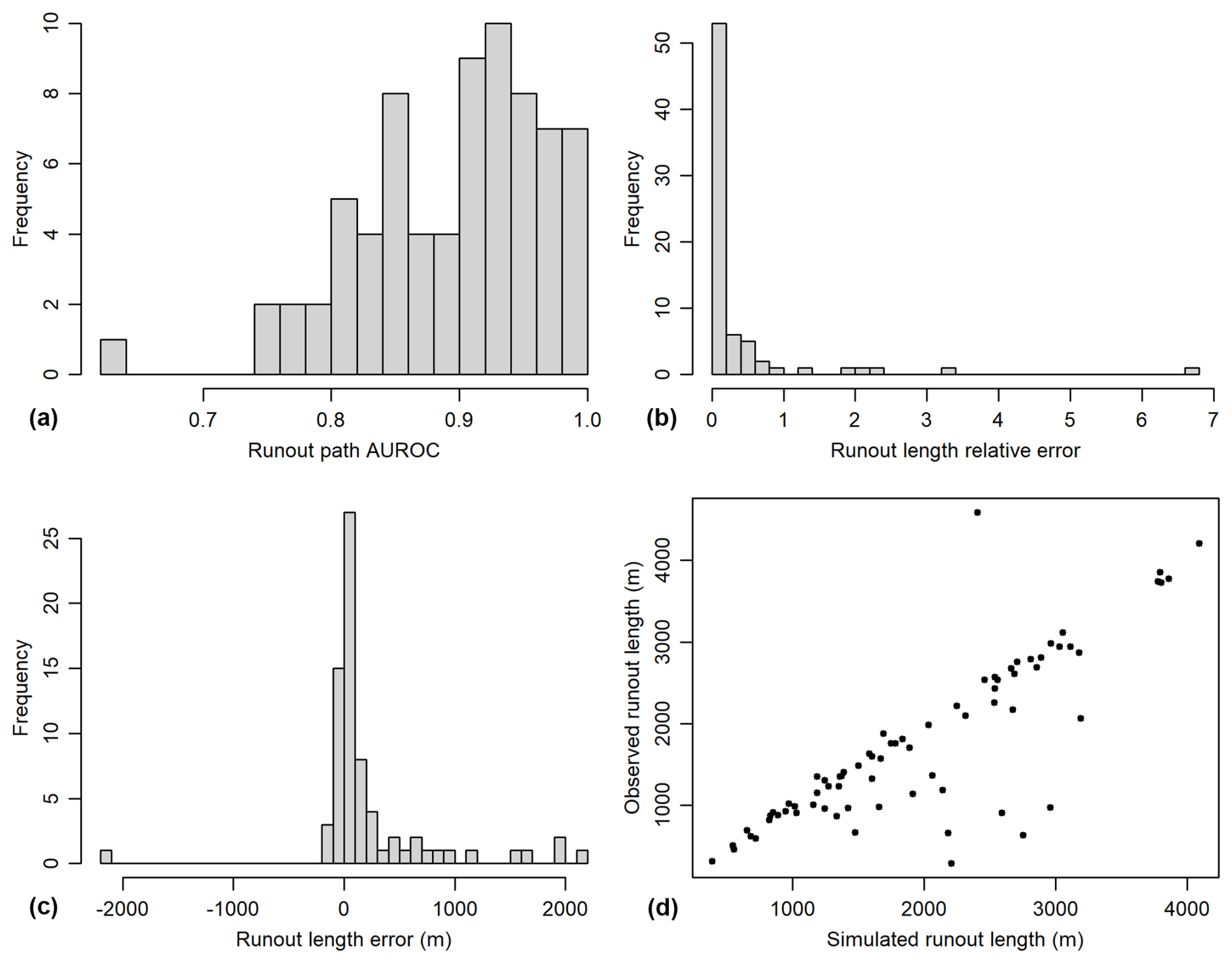
Figure 3 A histogram of the AUORC scores for the runout path (a). A histogram of the simulated runout length relative error with the optimal parameters (b). A histogram of the simulated runout length error with the optimal parameters (c). A plot of observed runout length versus the simulated runout length with the optimal parameters (d).

A qualitative assessment of the optimized runout performance comparing observed runout (used for model training) to the simulated runout paths, showed generally good agreement (Fig. 4). Deposition areas where debris flow momentum is lost, were often marked by lobate deposits or subtle terrain breaks at the distal end of previous events. The simulated runout distance was often greater (more conservative) than the observed runout paths (Fig. 3c and d). Individual cases where runout distance relative error was high, were due to situations random walks failed to “break through” sinks and narrow channels, which are artefacts of the DEM. The dispersion or spread of the runout paths also matches the observed runout paths. Since this is an example of general runout susceptibility, the aim was to at least capture the observed runout path polygon within the simulations. Likewise, visually comparing the modelling results with geomorphological features visible in the aerial imagery, the model was able to portray the extent of older flows, outside the observed/mapped runout. Thus, giving a more complete picture of potential flow paths, while confirming that the observed runout polygons are just one version of possible flow paths within the basin.

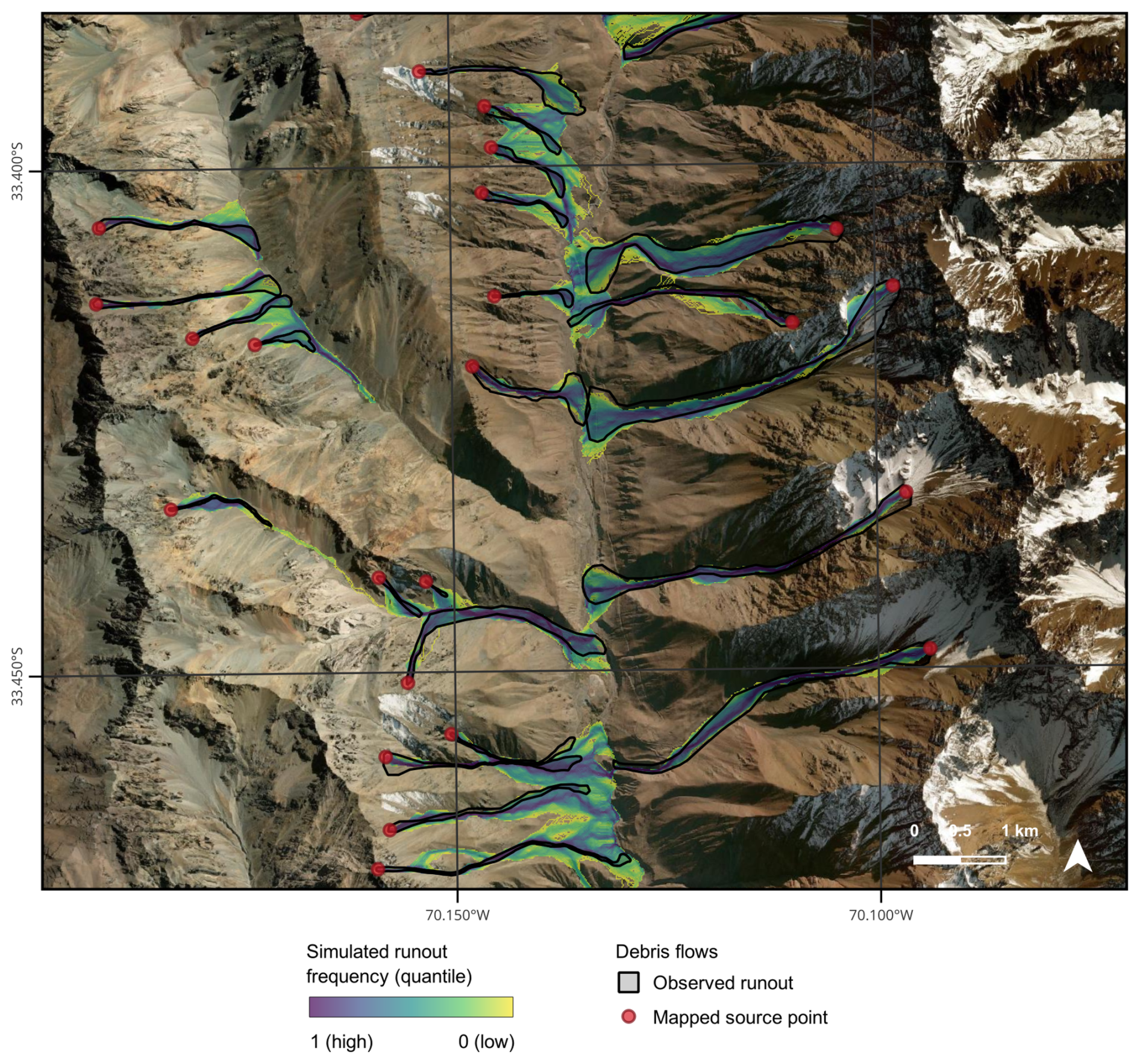
Figure 4 Map of observed and simulated runout from optimized regional model. Imagery sources: Esri, DigitalGlobe, GeoEye, i-cubed, USDA FSA, USGS, AEX, Getmapping, Aerogrid, IGN, IGP, swisstopo, and the GIS User Community – Powered by Esri.

3.6.2 Regional simulation of runout and source connectivity

The post-classification filtered source area prediction model classified 23 % of the study areas as a likely source for debris flows (Fig. 5a and b). These classified source areas were typically active scree slopes, steep slopes and gullies. Based on these classified source area grid cells, regionally simulated runout impacted 32 % of the basin (Fig. 6a). In total, 65 % (12 % of the basin) of source grid cells had a high probability (≥0.8) and 15 % (3 % of the basin) with no probability (0) of connectivity to the main river channel and stream network. The source grid cells with no connectivity were typically in high elevation areas dominated by peri-glacial and glacial processes, or in areas where levees have been formed next to the main river channel (Fig. 6b). In this case study, the higher connectivity probabilities show areas where sediment transportation to the main river channel and stream network is more likely to occur.

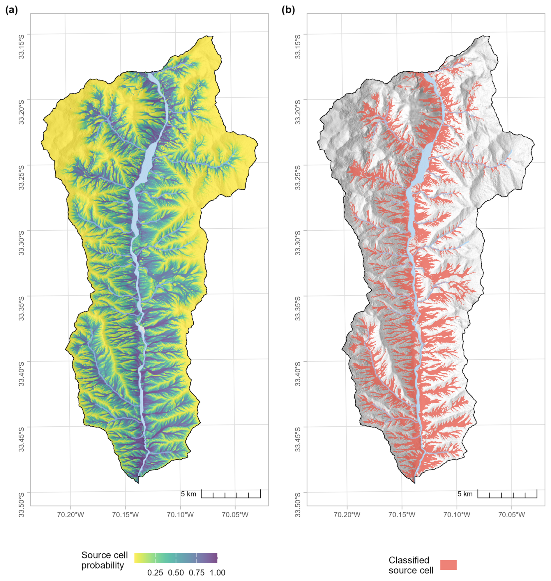
Figure 5 Map illustrating GAM predicted probabilities of being a source area (a) and the post-classification filtered source areas (b). The river and stream channel network are represented by the light blue polygons and lines.

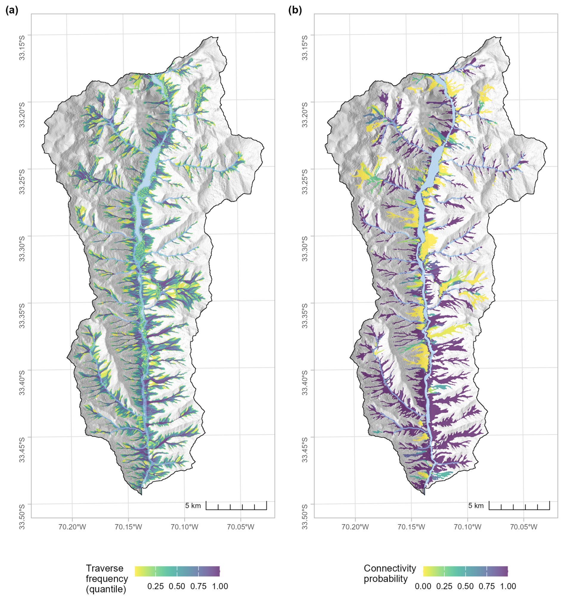
Figure 6 Map of regionally simulated debris flow runout from classified source cells (a); and source cell connectivity probability to the river and stream channel network (b). The river and stream channel network are represented by the light blue polygons and lines.

3.6.3 Computer processing and performance

All simulations were run on a Windows 10 Enterprise workstation equipped with an Intel^® Core™ i9-14900K processor (3.20 GHz, up to 6.0 GHz boost), with 25 cores (32 threads) and 128 GB of RAM. The analysis was based on a 6.5 MB DEM at 12.5 m resolution, covering 4 459 415 grid cells.

The random grid search optimization was parallelized across 30 threads. 73 mapped runout observations were each evaluated using 50 different parameter combinations, completing all simulations in approximately 15 min. The regional simulation included runout and connectivity modelling from 573 413 source cells, with 1000 random walks per grid source cell, and required approximately 16 h to complete. In both cases, memory usage per thread ranged between 450–710 MB, with total RAM usage peaking at ∼20 GB across all threads.

As a further example, simulating 73 mapped slides, each from a single corresponding source cell ranging in length from 290 to 4600 m, took approximately 2.3 min in total (about 2 s per slide on average) without any parallelization (e.g. producing the results in Fig. 4).

4 Discussion

4.1 General runout simulation assumptions

The runout modelling components in runoutSIM are built on a simplified set of assumptions that make them suitable for large-scale regional simulations. These include: (1) an unlimited supply of material from each source cell, (2) a static elevation model (i.e., the DEM is not updated during simulation to portray potential post event changes in the topography), and (3) sliding friction controls (which influence runout distance) can be defined globally or spatially.

Currently, all source cells are treated as transport-limited, meaning they have an unlimited supply of material. In the context of debris flows, estimating available material, whether through yield rate or erosion depth, is challenging due to its stochastic nature (Hungr et al., 2005). While supply estimates can improve model performance in post-event reconstruction (e.g. Bovis and Jakob, 1999), they are generally difficult to quantify a priori at regional scales, making predictive modelling with them impractical. As implemented, runoutSIM outputs the spatial probability of path traversal and runout extent (not volume) making it well-suited for identifying likely travel corridors, but less appropriate for sediment budgeting or volume-based hazard assessments.

Terrain is treated as static throughout the simulation. The model does not update the DEM to reflect erosion or deposition during runout. For coarser-resolution terrain data, this assumption is generally acceptable. However, for detailed, event-specific modelling, especially with high-resolution DEMs (<5 m), the model may become sensitive to small-scale terrain features. As others have shown, runout model outputs can vary significantly depending on the resolution and accuracy of the underlying DEM (Horton et al., 2013).

The default implementation of runoutSIM uses a global sliding friction coefficient, assuming a uniform, bare-earth surface. While this simplifies modelling, it overlooks the influence of surface roughness, vegetation, and land use. This limitation can be addressed by applying spatially distributed friction values (Goetz et al., 2025; Wichmann, 2017) and is supported within this R package (see Table 1).

4.2 Model calibration and parameter optimization

For the case study, a random grid search was implemented to optimize the random walk and PCM model components – allowing for quicker model tuning compared to exhaustive grid search approaches (Goetz et al., 2021). runoutSIM was intentionally developed without a built-in calibration framework, enabling users to customize optimization methods using R's existing libraries and adapt the process to their specific modelling needs.

4.3 A process-based model of connectivity

The connectivity probability index in runoutSIM allows us to estimate which downslope features, such as rivers, roads, or infrastructure, are likely to be impacted by landslides, and which upslope source areas are most likely to contribute to those impacts. This provides a more complete picture of runout behaviour, linking initiation zones with potential impact areas across the catchment. The runoutSIM approach is distinct in applying a process-based framework for modelling connectivity, rather than relying on empirical or rule-based assumptions (Shi et al., 2025). When working at large regional scales, any information that helps identifying priority areas, such as hillslopes that are both susceptible to release and well-connected to critical features, is extremely useful for hazard mitigation and planning. What is unique about this approach is that it provides a process-based framework for scenario building. For example, users can simulate runout connectivity under different sliding conditions, such as the presence or absence of forest cover (Goetz et al., 2025) and assess how these changes influence connectivity patterns.

The model also allows us to consider both general susceptibility to release (i.e., being a source area) and the probability of connectivity to downslope features. These can be adjusted using source area probabilities, which helps reduce overprediction of connectivity in areas with low initiation potential. This is important because not all potential source areas will connect with features of interest, and not all connected areas are equally likely to release material (Steger et al., 2022). By accounting for both components, we can better represent the spatial heterogeneity of initiation and source potential, and improve how we identify areas most relevant for hazard assessment and mitigation.

4.4 Computational considerations

Simulating runout from hundreds or thousands of source cells across large regions is computationally demanding. Even small case studies can require substantial processing time when modelling multiple flow paths per source. Parallelization helps improve performance but is constrained by available memory. Adding threads without sufficient RAM can reduce efficiency. For regional-scale applications, parallelization is generally necessary. For exploratory work or smaller case studies, sequential processing is often sufficient; especially when refining new optimization strategies.

To manage memory demands, runoutSIM stores only the frequency with which each cell is traversed, rather than the full set of individual simulation paths. While this limits the ability to visualize specific paths, it significantly reduces memory usage, making large-scale simulations feasible on a typical workstation. In theory, the model could be adapted to store complete paths, but this would be extremely memory-intensive.

4.5 Interactivity, practical deployment, and future development

One of the advantages of working entirely within R is the ease of sharing results using interactive maps. Mapped outputs can be saved as Leaflet-based HTML files, making it simple to share model results with collaborators or local experts for review and interpretation. This is especially useful for regional studies, where static maps often lack the detail needed for site-specific evaluation.

The framework of runoutSIM is also designed to support operational deployment. While meteorological thresholds can be applied where they are well established to hard-classify source areas for an event, the framework is designed to carry spatial likelihoods of initiation through the modelling chain, supporting the possibility of threshold-free runout forecasts.

The current implementation prioritizes code interpretability to make it easier for users to modify and extend the model. This comes at the cost of computational efficiency. If performance is a key requirement, like in operational forecasting, it may be worth translating core functions, like the random walk algorithm, to C$++$ using the Rcpp package (Eddelbuettel et al., 2025). However, doing so makes the code less transparent and harder to customize.

For research, training, and prototyping, the current R-based implementation should be sufficient. It supports rapid iteration, easy integration with other R packages, and flexible model development. Future improvements may focus on hybrid implementations that balance interpretability with performance, depending on the needs of the application, as well as wrapper functions to make it easier to swap modelling components. For example, wrapper functions that can substitute the current two-parameter friction model with energy line approaches or alternative friction models that would allow users to better match model complexity to the available data and computational requirements.

5 Conclusion

This paper introduced runoutSIM, an open-source R package for simulating the spatial extent, velocity, and connectivity of landslide runout at regional scales. By implementing random walk and process-based modeling techniques directly in R, runoutSIM provides a flexible and transparent environment for regional hazard assessment. The package enables users to streamline workflows, integrate statistical or machine learning models, and interactively visualize results.

The case study in the Río Olivares basin demonstrated how runoutSIM can be applied to optimize model parameters, predict source areas, and simulate runout connectivity to downslope features. Although the model is based on simplified assumptions to support large-scale simulations, it offers a solid foundation for continued development. Future work will focus on expanding process-based modeling options, improving calibration with empirical data, and integrating forecasting tools. By keeping the code open and modifiable, runoutSIM supports both research and applied use, allowing users to adapt the model to their own needs and contribute to advances in regional landslide modeling.