Simultaneous versus sequential estimation of biogeochemical and physical parameters in coupled marine ecosystem models

As computational resources have increased in availability and capability, so has the complexity of the models used to represent biogeochemical (BGC) processes in ocean simulations. To effectively calibrate the increasingly large number of uncertain parameters in these models, efficient parameter estimation methods are needed to ensure that the models can accurately represent the BGC processes under investigation. In this study, we address this challenge using a multistage automatic parameter estimation methodology that sequentially applies global sampling and local optimization to calibrate both the BGC model parameters and the parameters associated with a one-dimensional physical ocean model. We quantitatively compare the accuracy of sequential and simultaneous parameter estimations of moderately complex BGC and physical models at locations corresponding to the Bermuda Atlantic time series and the Hawaii Ocean time series. The results show that the best overall agreement with the observed mean seasonal cycles is obtained when BGC, advection, boundary condition, and turbulent diffusion parameters are estimated simultaneously, rather than sequentially. Simultaneous estimation of all these parameters results in closer agreement with mean seasonal cycles for oxygen and particulate organic nitrogen. Moreover, the agreement is improved in general when the advection, boundary condition, and turbulent diffusion parameters are included in the estimation, as opposed to calibrating the BGC model alone. This study also serves as a demonstration of a meta-algorithm for parameter estimation in high-dimensional models using a truncated global search with local optimizations.

1 Introduction

Computational simulations of the ocean on local, regional, and global scales typically rely on physical and biogeochemical (BGC) models whose parameters have been tuned using available observational data (e.g., temperature, current velocity, BGC tracer concentrations). The BGC, advection, boundary condition, and turbulent diffusion components of these coupled models, which represent complex physical and BGC processes across a range of spatiotemporal scales (Fox-Kemper and Ferrari, 2008; Henson et al., 2015; Smith et al., 2016; Ruiz et al., 2019), are often tuned sequentially in particular groupings, rather than simultaneously. As such, a tuning exercise for one group of model components may result in parameter values that compensate for errors introduced by estimating the parameters in another group of components. This type of sequential parameter estimation in coupled models may not produce accurate predictions of the coupled physical and BGC state under new or different ocean conditions, thereby reducing the general applicability and utility of the tuned model parameters. Although this challenge can be mitigated if there are a priori BGC or physical justifications for selecting the values of a subset of parameters, it is often the case that specific appropriate values are unknown and, at most, only acceptable parameter ranges can be defined.

As a first step in addressing this issue, we explore the potential benefits of simultaneous and fully coupled parameter estimations of model components by comparing sequential and simultaneous calibrations of a one-dimensional (1D), moderately complex, coupled BGC-physical model based on agreement with the mean seasonal cycle at two different ocean locations. The BGC model is the 17-state variable version of the Biogeochemical Flux Model (BFM17, Smith et al., 2021) and the physical model is the 1D formulation of the Princeton Ocean Model (POM1D, Blumberg and Mellor, 1987). This combined biophysical model (termed BFM17 + POM1D) was initially developed by Smith et al. (2021) from the 56-state variable BFM (Vichi et al., 2007) with parameter values that were manually adjusted to give good agreement with data for open ocean oligotrophic BGC conditions from the Bermuda Atlantic time series (BATS, Steinberg et al., 2001). Kern et al. (2024) further improved the accuracy and generality of BFM17 by developing and applying an efficient automated parameter estimation approach based on a three-step optimization method for BGC models with high-dimensional parameter spaces. Using the resulting optimized model, Kern et al. (2024) demonstrated good agreement between BFM17 + POM1D and the observed mean seasonal cycles from both BATS and the Hawaii Ocean time series (HOTS, Karl and Lukas, 1996).

Here, we employ the same three-step optimization method developed by Kern et al. (2024) to examine the relative benefits of sequential versus simultaneous estimations of parameters specific to the BGC model and parameters associated with the 1D physical model, which represent advection, boundary condition, and turbulent diffusion processes. The method treats parameter estimation as a constrained optimization problem using a global search followed by local gradient-based optimization. The use of local gradient-based optimization efficiently identifies an optimal solution, while the global search is used to avoid biasing the solution with ad hoc initial guesses. The best case among the optimized parameter sets is then selected as the optimal solution. Although this method previously resulted in a formulation of BFM17 + POM1D that agreed well with the observed mean seasonal cycles of BGC tracers available at BATS and HOTS, Kern et al. (2024) considered only the estimation of BGC model parameters, introducing the possibility that the BGC model was tuned to compensate for inaccuracies in the parameterization of physical processes. In the present study, we examine this issue by estimating 42 total parameters in the coupled biophysical model BFM17 + POM1D, comprising the 12 most sensitive parameters of the BGC model, 6 physical boundary condition and turbulence closure parameters, and 24 bimonthly vertical eddy mixing parameterization coefficients (also representing physical processes). We then quantitatively compare the accuracy of sequential versus simultaneous estimations of the BGC and physical model parameters at BATS and HOTS.

The paper is organized as follows. Section 2 provides a brief description of the parameter estimation methodology. The biophysical model BFM17 + POM1D is then described in Sect. 3. Results from the parameter estimations at the two observational locations are presented and discussed in Sect. 4. Finally, the main conclusions are presented in Sect. 5.

2 Optimization Methodology

The methodology used here was originally described in Kern et al. (2024) and treats parameter estimation as a constrained optimization problem, where a measure of the difference between the observed mean seasonal cycle and model output fields is minimized. A more complete description of the methodology is provided in Kern et al. (2024) and here we outline the specific implementation used in the present study. The parameter estimation problem is formulated as

$$\begin{array}{}\text{(1)}& \begin{array}{rl}& \underset{\mathit{c}}{min}{\sum }_{j=\mathrm{1}}^{N_{\mathrm{v}}}{\mathit{\delta }}_j\left(\mathit{c}\right)\\ & \text{subject to}{\mathit{c}}_{\min }\le \mathit{c}\le {\mathit{c}}_{\max },\end{array}\end{array}$$

where δ_j(c) is a measure of the disagreement between the model output and the mean seasonal cycle for a target field j, c is a vector of model parameters, and c_min and c_max are the minimum and maximum bounds, respectively, for c. We use phytoplankton chlorophyll, oxygen, nitrate, phosphate, and particulate organic nitrogen (PON) as our target fields, so N_v=5.

For the parameter estimation studies in Kern et al. (2024) and here, we quantify the difference between model and target data using the normalized root-mean-squared difference (RMSD), expressed as

$$\begin{array}{}\text{(2)}& {\mathit{\delta }}_j\left(\mathit{c}\right)={\displaystyle \frac{\mathrm{1}}{{\mathit{\sigma }}_j^{\left(\mathrm{obs}\right)}}}{\left\{\stackrel{\mathrm{‾}}{{\left[V_j^{\left(\mathrm{obs}\right)}(z,t)-V_j(z,t;\mathit{c})\right]}^{\mathrm{2}}}\right\}}^{\mathrm{1}/\mathrm{2}},\end{array}$$

where $V_j(z,t;\mathit{c})$ is the monthly-averaged, depth-dependent model output field for a given parameter set c and $V_j^{\left(\mathrm{obs}\right)}(z,t)$ is the corresponding target observational field. The overline in Eq. (2) indicates an average over all available depths and months and the RMSD is normalized by the standard deviation in the observational field over all depths and months, ${\mathit{\sigma }}_j^{\left(\mathrm{obs}\right)}$. Normalization with the standard deviation is primarily included to non-dimensionalize the RMSD values so they can be summed into a single objective value. Smaller values of δ_j(c) indicate lower error, with δ_j(c)=0 corresponding to identical observational and model fields for all depths and months. The case where δ_j(c)=1 corresponds to error between the observational and model fields that is the same as the variability in the observational field itself. In general, δ_j(c)≲1 is indicative of a good model fit to the observational data.

The parameter estimation methodology uses multiple local optimizations from initial points selected from the best of those included in a truncated global search. Although this approach does not guarantee a global minimum, it has the advantage of reducing the impact of arbitrary user decisions on optimization results. It consists of three primary steps:

1. The parameter space is probed N_samp times with a global search or optimization technique;

2. The N_top parameter sets are selected and used to initialize local optimization runs;

3. The results of the local optimizations are compared to select the final calibrated parameter set.

The methodology is very flexible in its most general form (Kern et al., 2024), leaving room for the selection of different sampling and optimization methods, the number of parameters sampled, and the number of local optimization runs.

The sampling and optimization are performed here with the coupled biophysical model using DAKOTA (Adams et al., 2019). DAKOTA is an open-source numerical toolbox that allows various sampling, optimization, and uncertainty quantification algorithms to be applied to an arbitrary model. Figure 1 is a schematic of BFM17 + POM1D, which will be discussed in the next section, and its coupling to DAKOTA. DAKOTA is able to apply a variety of algorithms to an arbitrary model by treating the model as a “black-box,” as indicated by the dashed line in Fig. 1. DAKOTA is not integrated with the model and instead interacts with the model through an interface program. DAKOTA outputs a set of parameters to be tested, runs the interface program, and then reads the value of the resulting objective function. The interface interprets the parameters, runs the simulation, and runs the objective function calculator.

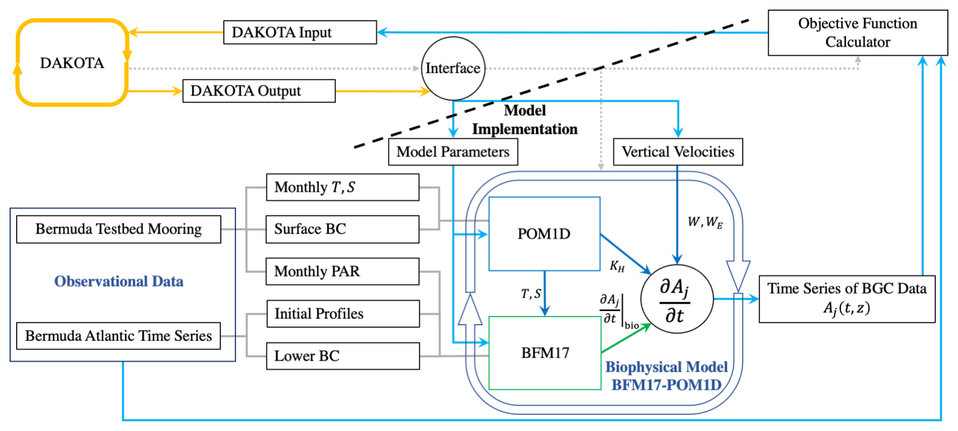
Figure 1 Schematic showing how DAKOTA interfaces with BFM17 + POM1D. The schematic also shows how BFM17 and POM1D are coupled. The schematic is for the BATS location, but is the same for HOTS except for the input data in the “Observational Data” box. The schematic is an edited version of one presented in Kern et al. (2024), now indicating that the optimization interface affects the BFM17, POM1D, and vertical velocity components of the biophysical model. The dashed line is used to indicate that DAKOTA treats the model as a black box and is only aware of the interface script controlling the model.

The parameter estimations performed here use the standard Latin Hypercube Sampling algorithm from DAKOTA for Step 1. The local optimizations (Step 2) are performed using a Quasi-Newton (QN) algorithm provided by the Opt$++$ library within DAKOTA (Meza et al., 2007). Opt$++$ is a C$++$ class library that uses object-oriented programming for nonlinear optimization algorithms. The object-oriented toolbox provides a relatively simple way to select different modules that set the optimizer and its behavior in a manner consistent with the larger DAKOTA framework. The QN method was used in Kern et al. (2024) after testing various algorithms available in DAKOTA. It performed the best by reliably and efficiently converging to a solution. Other algorithms, especially conjugate gradient, were not able to converge either efficiently or at all due to the topography of the objective space. It should be noted that because this methodology includes an initial step in which the parameter space is randomly sampled, repeated applications of the methodology with different random samples could lead to different results. With enough random samples, however, confidence in the repeatability of the results improves, but this must be balanced against the computational cost of sampling many random points, the majority of which will not be used for subsequent gradient-based optimizations. Additional details on DAKOTA, as well as how it can be downloaded, are available at https://dakota.sandia.gov (last access: 15 May 2026). The present implementation of the parameter estimation method in DAKOTA is available at Kern et al. (2025a), with an additional description of the use of DAKOTA in Kern et al. (2024).

In the present study, we explore the sequential versus simultaneous optimization of 42 total model parameters representing BGC, advection, boundary control, and turbulent diffusion processes within the coupled biophysical model described in the following section. These tests are performed separately at two different ocean locations corresponding to the BATS and HOTS observational datasets. Sequential calibration studies are performed by applying the parameter estimation methodology first to the parameters associated with the physical model, including advection, boundary control, and turbulent diffusion parameters, beginning with the baseline values in Smith et al. (2021). The parameters that produce the best overall agreement are then used as the starting point in another calibration of the 12 exclusively BGC parameters identified as the most important according to a sensitivity analysis (described in Appendix A). In each estimation step, sampling is performed for N_samp=10 000 randomly generated parameter sets to increase the repeatability of the results without incurring excessive computational cost. Then, the gradient-based optimization algorithm is applied to the N_top=20 best-performing parameter sets.

The simultaneous calibration case estimates the complete set of parameters of the coupled model at the same time, starting from the baseline parameters in Smith et al. (2021). For these cases, initial sampling is performed with N_samp=20 000 random parameter sets. The sampling in this case is intended to match the total number of samples applied to obtain the final solution in the sequential calibration case. We still apply the optimization algorithm to the N_top=20 best-performing parameter sets.

The number of randomly sampled sets of parameters for sequential and simultaneous optimization cases is determined primarily on the basis of available computational resources. Because there are 42 parameters, we cannot fully explore the objective function space and therefore limit the samples based on available user and compute time. The number of parameter sets used to initialize the gradient-based optimizations is based on similar reasoning; however, the analysis included in Appendix B of Kern et al. (2024) suggests that N_top=20 should be sufficient.

3 Model Description

The biophysical model used in this study, BFM17 + POM1D (Smith et al., 2021), tracks 17 BGC tracers in a depth-dependent column of water over time. The time-rate of change for a state variable, A_j, in the model is described by

$$\begin{array}{}\text{(3)}& \begin{array}{rl}{\displaystyle \frac{\partial A_j}{\partial t}}& ={\left.{\displaystyle \frac{\partial A_j}{\partial t}}\right|}_{\mathrm{bio}}-\left[W+W_{\mathrm{E}}-v^{\left(\mathrm{set}\right)}\right]{\displaystyle \frac{\partial A_j}{\partial z}}\\ & +{\displaystyle \frac{\partial }{\partial z}}\left(K_{\mathrm{H}}{\displaystyle \frac{\partial A_j}{\partial z}}\right),\end{array}\end{array}$$

where the various components of this equation are described in more detail in the following sections. Broadly, the three terms on the right-hand side of the equation correspond to BGC dynamics, vertical advection, and turbulent mixing, respectively. In this study, we consider the parameters associated with the first term to be the exclusively BGC parameters that would also be present in a zero-dimensional (i.e., time-only) implementation of the model. The last two terms represent advection and turbulent diffusion processes, respectively. The parameters associated with these processes, along with the boundary condition parameters, are only introduced when the BGC model is coupled to POM1D. As such, these parameters are considered to be associated with the physical model, although their values may be specific to certain BGC species, particularly in the case of the settling velocity and the boundary conditions.

3.1 Biogeochemistry

The first term on the right-hand side of Eq. (3) is the rate of change due to BGC processes, which is modeled here using BFM17. This model is a simplified implementation of the complete BFM (Vichi et al., 2007), which itself uses a chemical functional family (CFF) approach to model BGC communities. This framework models different BGC communities by including or excluding ecosystem components based on their prevalence in the target community. Previous implementations of the model have included 56 state variables and the benthic system for studying the vertical structure of BGC communities in coastal regions. In Smith et al. (2021), the 17 state variable implementation was developed to represent open-ocean oligotrophic BGC communities while being computationally affordable for implementation in high-resolution simulations of small to submesoscale ocean dynamics. Previous studies used BFM coupled with POM1D (Vichi et al., 2003; Mussap et al., 2016; Mussap and Zavatarelli, 2017a, b), but with the smaller implementation of BFM, we can also couple the BGC model to more complex physical models.

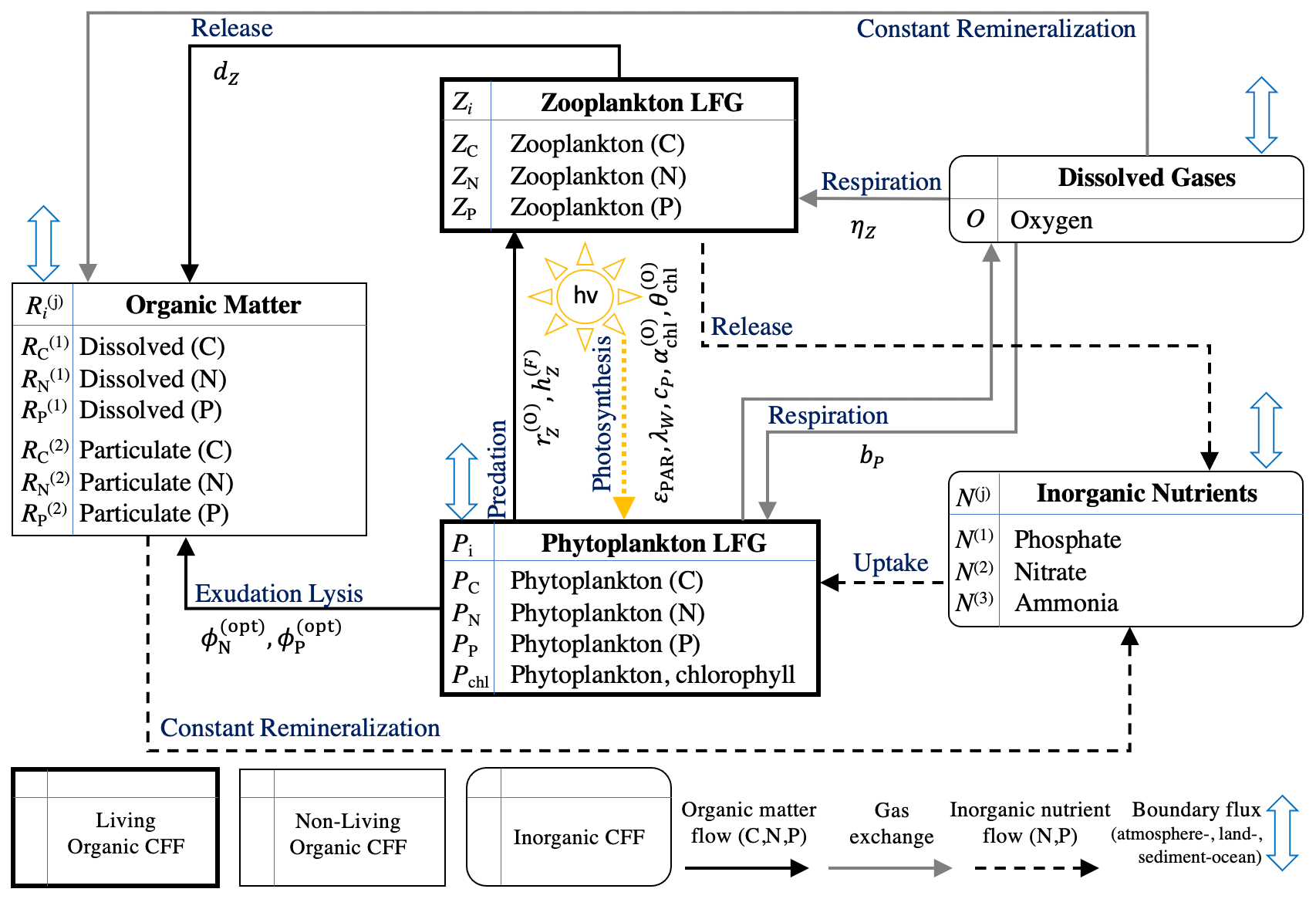
Figure 2 Schematic of the Biogeochemical Flux Model with 17 state variables (BFM17). The schematic lists all 17 state variables and shows the flux pathways between different chemical functional families (CFF). The schematic was originally presented in Smith et al. (2021). The diagram has been updated to show the included BGC parameters (listed in Table 1) associated with each flux pathway.

Compared to the full BFM, the formulation of BFM17 removes components based on assumptions appropriate for open ocean oligotrophic conditions (i.e., the benthic system, iron cycle, silicate cycle, and bacteria) and introduces generalized living functional groups (LFGs) representing community average behavior instead of specific types of phytoplankton or zooplankton. Figure 2 shows all 17 state variables with parameterized flux pathways. The model includes a general phytoplankton LFG, a general zooplankton LFG, dissolved non-living organic matter, particulate non-living organic matter, three inorganic nutrients, and the dissolved gas oxygen.

Modeled BGC tracers include the constituent elements carbon, nitrogen, and phosphorus, with zooplankton, dissolved non-living organic matter, and particulate non-living organic matter each having three state variables. Phytoplankton has the additional state variable chlorophyll, due to the importance of chlorophyll dynamics and the availability of observational data for it. There are three inorganic nutrients included in BFM17: phosphate, nitrate, and ammonia. Each has one tracer element (phosphorus, nitrogen, and nitrogen, respectively), and therefore each contributes only one additional state variable to the model. The dissolved gas oxygen is tracked in the model, while carbon dioxide is treated as an infinite source or sink as needed.

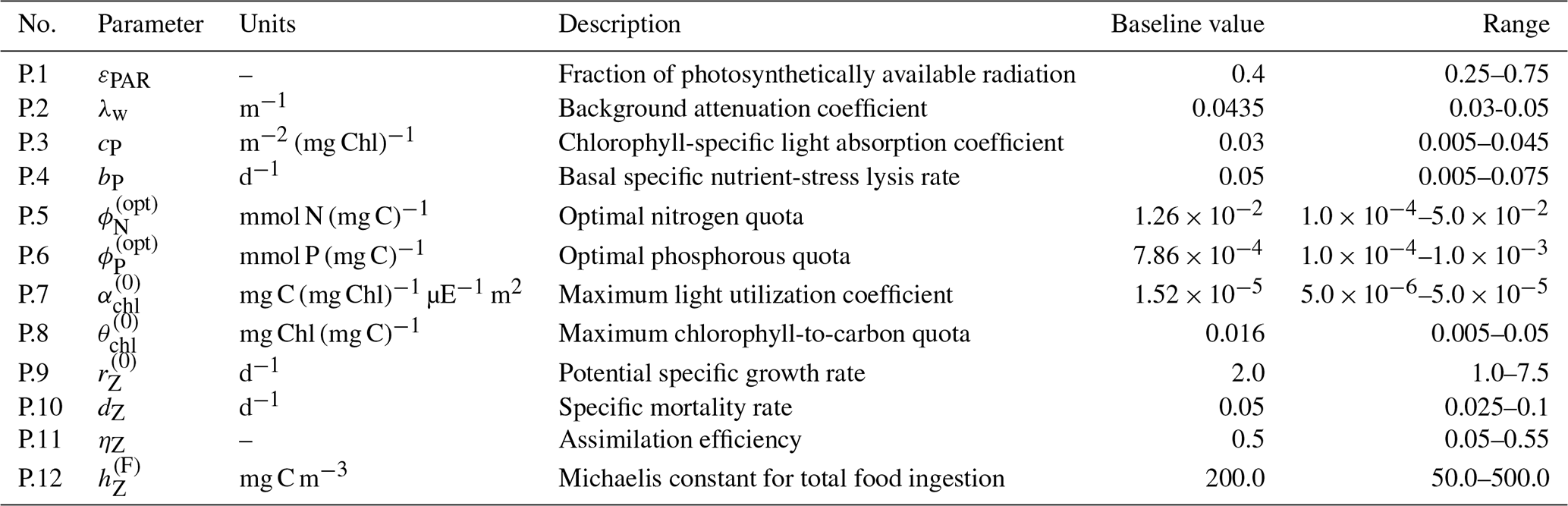
A general discussion of BFM and the CFF approach is available in Vichi et al. (2007) and a full description of BFM17 and the included dynamics is available in Smith et al. (2021). With the formulation of BFM17 using generalized phytoplankton and zooplankton LFGs, re-evaluating parameter values is essential. The values that could be applied consistently for particular species must be tuned to a particular community to represent its average behavior. Although the parameters of the BGC model are estimated in Kern et al. (2024), in this study we begin with the baseline parameters of Smith et al. (2021). The same baseline parameters are used for both locations considered in the present study. The parameter estimations here prioritize only the most sensitive BGC parameters included in Table 1 instead of simultaneously estimating them all. The sensitivity study in Appendix A was used to determine the 12 BGC parameters included in our estimation cases. The upper and lower parameter bounds are informed by supplementary material from Vichi et al. (2007) and the study by Kern et al. (2024). The twin simulation experiments (TSEs) in Appendix B further show how well the present methodology is able to recover the values of these parameters when perturbing the model from its baseline values.

Table 1 List of the 12 most important BFM17 parameters according to the sensitivity analysis in Appendix A; these are the BGC parameters included in the parameter estimation tests.

3.2 Vertical advection

The second term on the right-hand side of Eq. (3) describes the effect of advection on the vertical transport of BGC state variables by the seasonal general circulation (W), mesoscale eddies (W_E), and the variable-dependent settling velocity (v^(set)). The general circulation is assumed to result from Ekman pumping in a parameterization similar to the method employed by Bianchi et al. (2006). The corresponding monthly vertical profiles of W are shown in Smith et al. (2021) for the BATS location, where the velocity is zero at the surface and reaches a largest negative value near the bottom of the Ekman layer, which is assumed here to correspond to the bottom of the model domain. The largest magnitude negative velocity is calculated as (Smith et al., 2021)

$$\begin{array}{}\text{(4)}& W_{\max }=\widehat{k}\cdot \mathbf{\nabla }\times \left({\displaystyle \frac{{\mathit{\tau }}_{\mathrm{w}}}{\mathit{\rho }f}}\right),\end{array}$$

where τ_w is the wind stress, ρ is the density, and f is the Coriolis parameter. The curl of the wind stress is calculated using observational data. The resulting profiles of W for BATS and HOTS are all negative, resulting in purely downward advection due to the general circulation.

In contrast to the monthly profiles of W, mesoscale eddies provide vertical velocity perturbations on the time scale of weeks. In the present work, these advection events are parameterized by multiplying the monthly profiles of W, denoted W_m(z) for month m, by a randomly generated coefficient such that the maximum vertical eddy velocity is between 0.0 and 0.1 md⁻¹. This is expressed by the equation

$$\begin{array}{}\text{(5)}& W_{\mathrm{E},m}^{\left(k\right)}\left(z\right)=C_m^{\left(k\right)}{W}_m\left(z\right),\end{array}$$

where $W_{\mathrm{E},m}^{\left(k\right)}\left(z\right)$ is the vertical eddy velocity profile for month m with k=1 indicating the first half of each month and k=2 the second half. As a result, the general circulation W is defined monthly, but the eddy velocity profiles W_E are defined semi-monthly. The entire general circulation profile for a given month, m, is multiplied by a single coefficient, $C_m^{\left(k\right)}$. The vertical profile of the general circulation velocity at each time step is linearly interpolated from the monthly average profiles, while the eddy velocity profiles remain constant throughout their 15 d period.

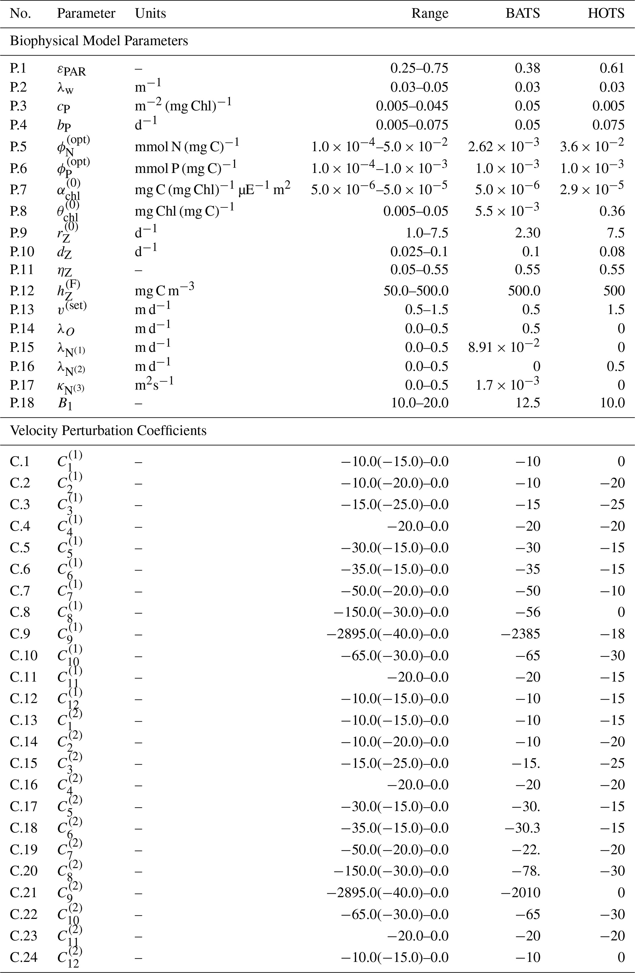
Although the 24 coefficients $C_m^{\left(k\right)}$ used to generate the eddy velocity profiles were initially generated randomly in Smith et al. (2021), here we treat them as parameters to be estimated. The initial coefficient values taken from the randomly generated baseline values in Smith et al. (2021) are included in Table 2, as are the upper and lower bounds used as constraints during the parameter estimation. Note that the initial values have been rounded and the upper and lower bounds were set to allow for maximum eddy velocities between 0.0 and 0.2 m d⁻¹, thereby relaxing the original assumption limiting them to 0.1 m d⁻¹.

Table 2 List of vertical advection, boundary condition, and turbulent diffusion model parameters with baseline values from Smith et al. (2021) and Kern et al. (2024) for the BATS and HOTS locations, respectively, along with parameter ranges used during the estimation process.

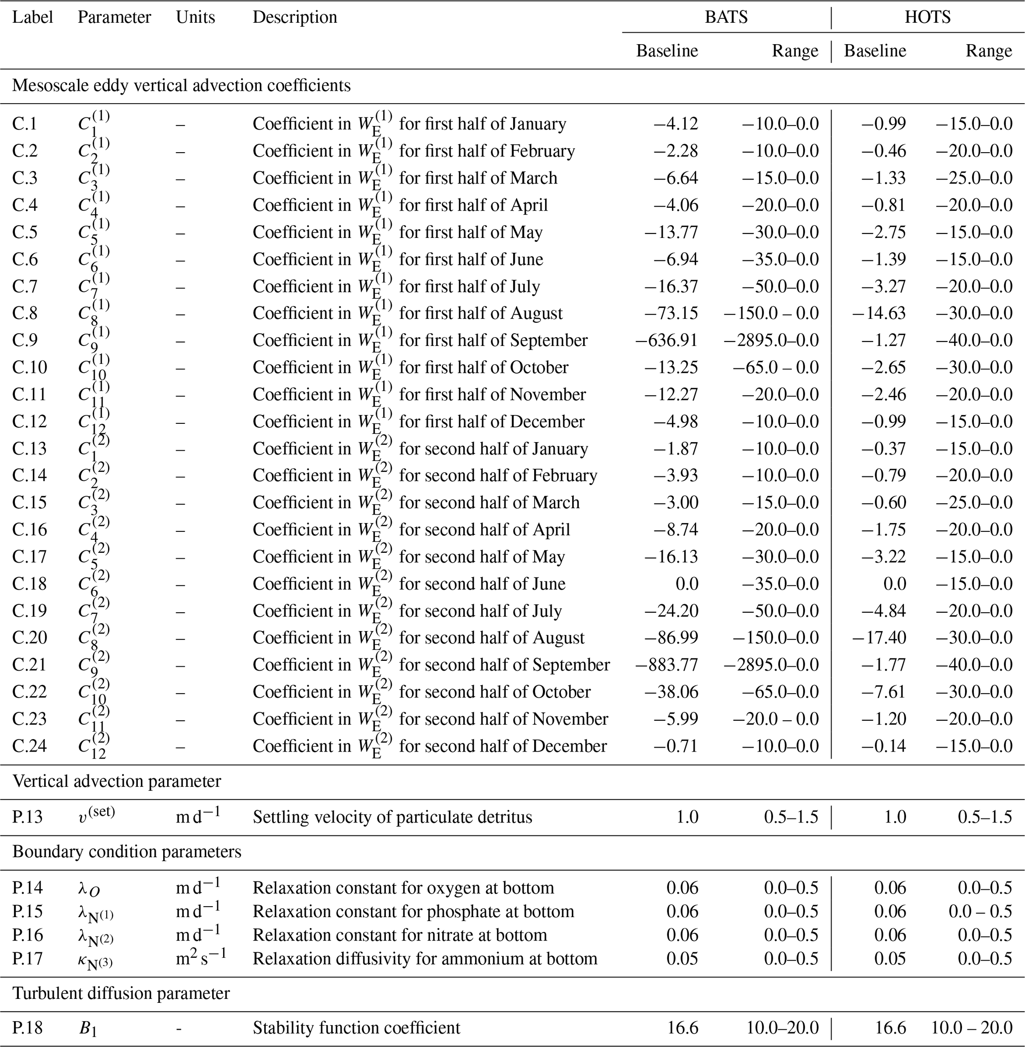
The final component in the vertical advection term on the right hand side of Eq. (3) is the state variable-dependent settling velocity, v^(set). The settling velocity is zero for all BGC state variables except non-living particulate organic matter, for which it has a constant non-zero value at all depths. This parameter is included in Table 2.

3.3 Boundary conditions

The BGC model includes boundary conditions for the top and bottom of the water column. For all state variables except oxygen, the flux at the surface is assumed to be zero. The flux at the bottom of the domain is also assumed to be zero for phytoplankton, zooplankton, dissolved non-living organic matter, and particulate non-living organic matter. The surface boundary condition for oxygen is a parameterized air-sea gas flux (Φ_O), defined as

$$\begin{array}{}\text{(6)}& {\left.K_{\mathrm{H}}{\displaystyle \frac{\partial O}{\partial z}}\right|}_{z=\mathrm{0}}={\mathrm{\Phi }}_{\mathrm{O}},\end{array}$$

which is based on the method developed in Wanninkhof (1992, 2014).

The bottom boundary conditions for oxygen, phosphate, and nitrate are given by the equation

$$\begin{array}{}\text{(7)}& {\left.K_{\mathrm{H}}{\displaystyle \frac{\partial A_j}{\partial z}}\right|}_{z=z_{\mathrm{end}}}={\mathit{\lambda }}_j\left({\left.A_j\right|}_{z=z_{\mathrm{end}}}-A_j^{*}\right),\end{array}$$

where λ_j is the corresponding relaxation velocity. The reference state variable $A_j^{*}$ is the value of the climatological field observed at the bottom boundary. The bottom boundary condition for ammonium is

$$\begin{array}{}\text{(8)}& {\left.K_{\mathrm{H}}{\displaystyle \frac{\partial A_j}{\partial z}}\right|}_{z=z_{\mathrm{end}}}={\mathit{\kappa }}_{{\mathrm{N}}^{\left(\mathrm{3}\right)}}{\left.{\displaystyle \frac{\partial Q_{\mathrm{N}}}{\partial z}}\right|}_{z=z_{\mathrm{end}}},\end{array}$$

where Q_N is the PON, defined as the total particulate organic matter from phytoplankton, zooplankton, and the particulate non-living organic matter in terms of nitrogen; that is $Q_{\mathrm{N}}=P_{\mathrm{N}}+Z_{\mathrm{N}}+R_{\mathrm{N}}^{\left(\mathrm{2}\right)}$. The ammonia boundary condition returns nitrogen from depth in the form of ammonium, where particulate organic matter is recycled to the inorganic nutrient. The boundary condition is modulated by the diffusivity of ammonia, ${\mathit{\kappa }}_{{\mathrm{N}}^{\left(\mathrm{3}\right)}}$.

Although the top boundary condition for oxygen is considered to be well-defined, there are four uncertain parameters at the bottom boundary: the three relaxation coefficients for oxygen, phosphate, and nitrate and the diffusivity for ammonia. These parameters are included in Table 2 because of their role in coupling the BGC and physical dynamics at the bottom boundary, as well as their connection to the 1D physical model.

3.4 Turbulent diffusion

The final term on the right-hand side of Eq. (3) represents turbulent diffusion in the vertical direction. This part of the model has been adapted from the three-dimensional (3D) version of POM. Turbulent diffusion is parameterized by introducing a turbulent eddy viscosity, K_M, and a turbulent eddy diffusivity, K_H. The latter quantifies the effect of turbulent mixing on state variables in the state variable transport equation.

The POM1D closure model is proposed in Mellor (2001) as a particular implementation of the one originally developed in Mellor and Yamada (1982). A discussion of the model as it is coupled to BFM17 is included in Smith et al. (2021). The closure model parameterizes the turbulent eddy viscosity and diffusivity as

$$\begin{array}{}\text{(9)}& {\displaystyle }{K}_{\mathrm{M}}=q\mathrm{\ell }{S}_{\mathrm{M}},\text{(10)}& {\displaystyle }{K}_{\mathrm{H}}=q\mathrm{\ell }{S}_{\mathrm{H}},\end{array}$$

where q is the turbulent velocity, ℓ is the master length scale, and S_M and S_H are stability functions written as

$$\begin{array}{}\text{(11)}& {\displaystyle }\begin{array}{rl}{S}_{\mathrm{M}}\left[\mathrm{1}-\mathrm{9}{A}_{\mathrm{1}}{A}_{\mathrm{2}}{G}_{\mathrm{H}}\right]& -S_{\mathrm{H}}\left[\left(\mathrm{18}{A}_{\mathrm{1}}^{\mathrm{2}}+\mathrm{9}{A}_{\mathrm{1}}{A}_{\mathrm{2}}\right)G_{\mathrm{H}}\right]\\ & =A_{\mathrm{1}}\left[\mathrm{1}-\mathrm{3}{C}_{\mathrm{1}}-\mathrm{6}{A}_{\mathrm{1}}/B_{\mathrm{1}}\right],\end{array}\text{(12)}& {\displaystyle }{S}_{\mathrm{H}}\left[\mathrm{1}-\left(\mathrm{3}{A}_{\mathrm{2}}{B}_{\mathrm{2}}+\mathrm{18}{A}_{\mathrm{1}}{A}_{\mathrm{2}}\right)G_{\mathrm{H}}\right]=A_{\mathrm{2}}\left[\mathrm{1}-\mathrm{6}{A}_{\mathrm{1}}/B_{\mathrm{1}}\right].\end{array}$$

The coefficients in the stability functions (i.e., $A_{\mathrm{1}},B_{\mathrm{1}},A_{\mathrm{2}},B_{\mathrm{2}},C_{\mathrm{1}}$) are constants and

$$\begin{array}{}\text{(13)}& G_{\mathrm{H}}={\displaystyle \frac{{\mathrm{\ell }}^{\mathrm{2}}}{q^{\mathrm{2}}}}{\displaystyle \frac{g}{{\mathit{\rho }}_{\mathrm{0}}}}{\displaystyle \frac{\partial \mathit{\rho }}{\partial z}}.\end{array}$$

Our implementation of BFM17 + POM1D uses imposed temperature, T, and salinity, S, profiles from observational data to calculate the vertical density profile. Temperature and salinity are interpolated from monthly profiles at each time step. Given the vertical structure of the ocean state, the model calculates the vertical diffusivity using transport equations for the turbulence parameters q and ℓ. The governing equation for the turbulent kinetic energy, $q^{\mathrm{2}}/\mathrm{2}$, is

$$\begin{array}{}\text{(14)}& \begin{array}{rl}{\displaystyle \frac{\partial }{\partial t}}\left({\displaystyle \frac{q^{\mathrm{2}}}{\mathrm{2}}}\right)& ={\displaystyle \frac{\partial }{\partial z}}\left[K_q{\displaystyle \frac{\partial }{\partial t}}\left({\displaystyle \frac{q^{\mathrm{2}}}{\mathrm{2}}}\right)\right]+K_{\mathrm{M}}\left[{\left({\displaystyle \frac{\partial U}{\partial z}}\right)}^{\mathrm{2}}\right.\\ & \left.+{\left({\displaystyle \frac{\partial V}{\partial z}}\right)}^{\mathrm{2}}\right]+{\displaystyle \frac{g}{{\mathit{\rho }}_{\mathrm{0}}}}{K}_{\mathrm{H}}{\displaystyle \frac{\partial \mathit{\rho }}{\partial z}}-{\displaystyle \frac{q^{\mathrm{3}}}{B_{\mathrm{1}}\mathrm{\ell }}},\end{array}\end{array}$$

while the governing equation for the master length scale, ℓ, is

$$\begin{array}{}\text{(15)}& \begin{array}{rl}{\displaystyle \frac{\partial }{\partial t}}\left(q^{\mathrm{2}}\mathrm{\ell }\right)& ={\displaystyle \frac{\partial }{\partial z}}\left[K_q{\displaystyle \frac{\partial }{\partial t}}\left(q^{\mathrm{2}}\mathrm{\ell }\right)\right]+E_{\mathrm{1}}\mathrm{\ell }{K}_{\mathrm{M}}\left[{\left({\displaystyle \frac{\partial U}{\partial z}}\right)}^{\mathrm{2}}\right.\\ & \left.+{\left({\displaystyle \frac{\partial V}{\partial z}}\right)}^{\mathrm{2}}\right]+E_{\mathrm{1}}\mathrm{\ell }{\displaystyle \frac{g}{{\mathit{\rho }}_{\mathrm{0}}}}{K}_{\mathrm{H}}{\displaystyle \frac{\partial \mathit{\rho }}{\partial z}}+{\displaystyle \frac{q^{\mathrm{3}}}{B_{\mathrm{1}}}}\stackrel{\mathrm{̃}}{W}.\end{array}\end{array}$$

In these equations, K_q=κK_H is a vertical diffusivity for the turbulent parameters and $\stackrel{\mathrm{̃}}{W}=\left[\mathrm{1}+E_{\mathrm{2}}{l}^{\mathrm{2}}/{\mathit{\kappa }}^{\mathrm{2}}\left(\right|z{|}^{-\mathrm{1}}+|z-H{|}^{-\mathrm{1}}{)}^{\mathrm{2}}\right]$ is a surface proximity function. Equation (15) and the surface proximity function include the nondimensional parameters E₁ and E₂, whose values have been included in Table C1.

In the above equations, g=9.81 m s⁻¹ is gravity, ρ₀=1025 kg m⁻³ is the reference density, and κ=0.4 is the Von Kármán constant. The horizontal velocity components, U and V, are obtained by solving the momentum equations

$$\begin{array}{}\text{(16)}& {\displaystyle \frac{\partial U}{\partial t}}-fV={\displaystyle \frac{\partial }{\partial z}}\left(K_{\mathrm{M}}{\displaystyle \frac{\partial U}{\partial z}}\right),\text{(17)}& {\displaystyle \frac{\partial V}{\partial t}}-fU={\displaystyle \frac{\partial }{\partial z}}\left(K_{\mathrm{M}}{\displaystyle \frac{\partial V}{\partial z}}\right),\end{array}$$

where f is the Coriolis parameter.

There are seven prescribed parameters in this model: the five coefficients included in the stability functions and the two non-dimensional parameters E₁ and E₂. The values of these parameters were determined in Mellor and Yamada (1982) and are included in Table C1. Since these coefficients parameterize the local turbulent dynamics, they are treated in this paper as unknown parameters that can be estimated. Ultimately, only one of these parameters (B₁) is included in our parameter estimation because of its relative importance in affecting model outputs, as shown in Table 2.

3.5 Model setup

Each simulation is run for 3 years with a time step of 400 s while state variable data was output as a daily average value. The initial conditions correspond to January values for chlorophyll, particulate organic nitrogen, oxygen, nitrate, and phosphate. The remaining state variable values are determined from the Redfield ratio (Redfield et al., 1963) or are assumed to have low initial values. By the beginning of the third year, the initial conditions are forgotten and monthly averages can be calculated from the daily data. The represented water column is the top 150 m of the ocean with the numerical domain consisting of 1 m grid spacing.

Monthly averages of salinity, temperature, and wind speed were used to force BFM17 + POM1D. The climatological salinity and temperature data were imposed to prevent energy drift common to 1D models. The wind data were taken from the Scatterometer Climatology of Ocean Winds database (Risien and Chelton, 2008).

4 Results and Discussion

In this study, we calibrate BFM17 + POM1D at two locations corresponding to the mid-Atlantic and the subtropical Pacific. Observational data from the Bermuda Testbed Mooring (Dickey et al., 2001) and BATS (Steinberg et al., 2001) are available for the former location, while data from HOTS (Karl and Lukas, 1996) are available for the latter. Both BATS and HOTS have long observational records for BGC and physical quantities, and we averaged the data over all available years to obtain monthly climatological depth-dependent profiles that were then fitted to a 1 m grid for the top 150 m of the ocean. In both cases, BGC data for phytoplankton chlorophyll, oxygen, nitrate, phosphate, and PON were used as target data for the biophysical model outputs. These five fields were selected because they are included in both the BATS and HOTS datasets, thereby providing a consistent set of inputs and outputs for the two locations.

The calibration of the complete set of BGC parameters, as well as the boundary condition parameters, was examined and described for the BATS and HOTS locations in Kern et al. (2024). In the following, we compare results from sequential and simultaneous estimations of the advection, boundary condition, and turbulent diffusion parameters, and then BGC parameters, at both locations.

4.1 Bermuda Atlantic time-series (BATS)

Observational and model data for the target fields at the BATS location are shown in Fig. 3, with concentrations of phytoplankton chlorophyll, oxygen, nitrate, phosphate, and PON provided as functions of month and depth. The observational data in Fig. 3a shows that the subsurface maximum in phytoplankton chlorophyll is observed between 50 and 100 m for most of the year. A spring bloom is observed in the annual cycle of phytoplankton, resulting in increased growth as deeper mixing provides nutrients to the surface layer. During the summer months, the water column is more stratified, the subsurface maximum is pushed deeper, and the overall extent and magnitude of phytoplankton chlorophyll decreases. Oxygen generally fills the domain with lower concentrations at the top and bottom of the water column during the latter half of the year. Nitrate and phosphate have high concentrations at a depth of 150 m and lower concentrations in the upper water column due to the biological pump. Both have a slight increase in concentration from November through January. The PON is largely confined to the top of the domain where the BGC community is most active. Similar to the seasonal cycle in phytoplankton, the subsurface maximum in PON shoals April through November.

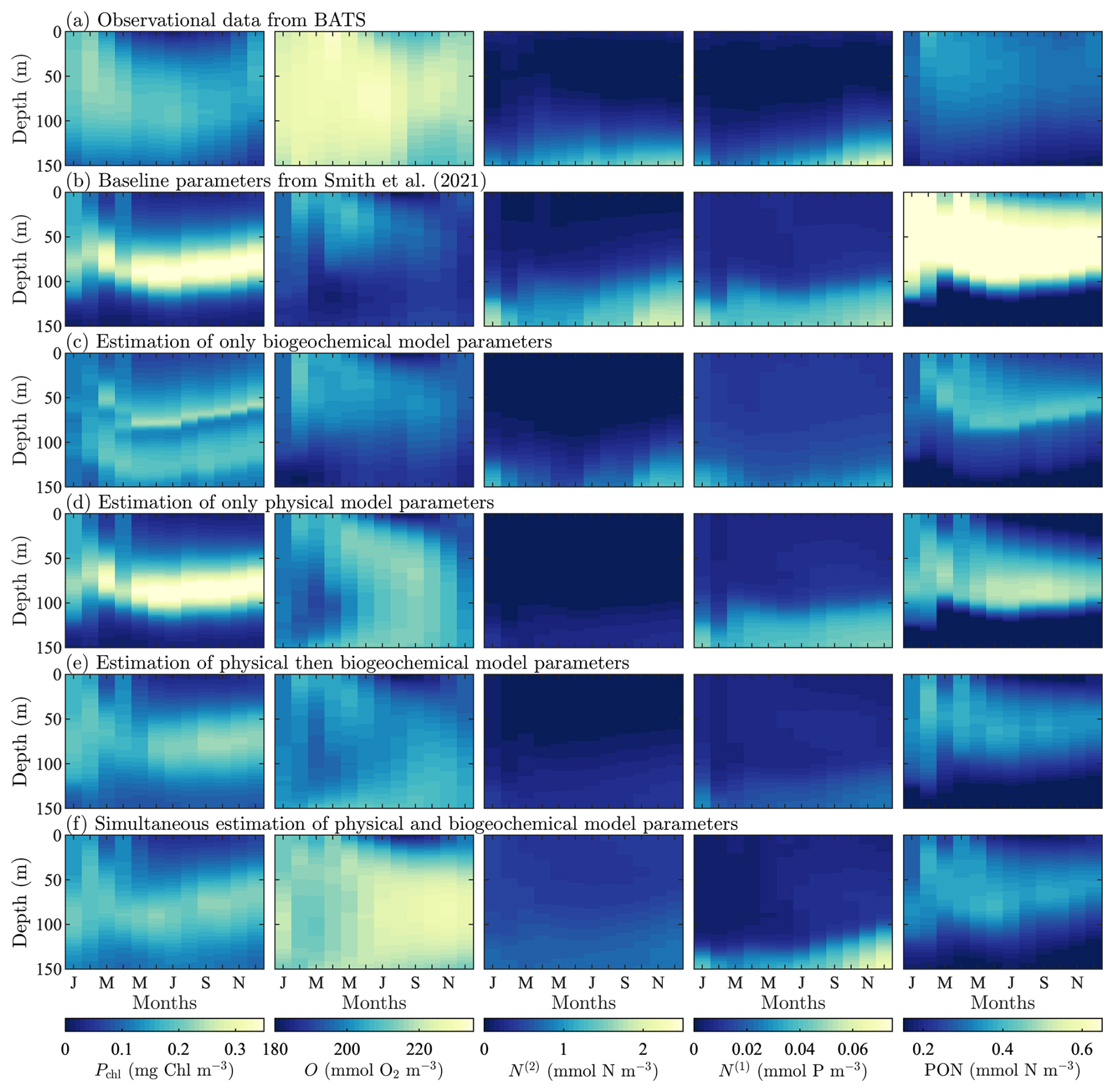
Figure 3 BATS observational and model results for target-field concentration data for (from left-to-right) phytoplankton chlorophyll (P_chl), oxygen (O), nitrate (N⁽²⁾), phosphate (N⁽¹⁾), and particulate organic nitrogen (PON). Row (a) is the reference observational data and subsequent rows correspond to model runs with the parameter values from Smith et al. (2021) (b), estimated BGC parameters only (c), estimated parameters in the physical model only (d), sequentially estimated parameters (e), and simultaneously estimated parameters (f).

Baseline model results from the original formulation of BFM17 + POM1D in Smith et al. (2021) are shown in Fig. 3b. Although the baseline model fails to predict the magnitudes of the observational data, it produces a similar behavior in the seasonal cycle for each of the target fields. At the subsurface maximum throughout the year, the modeled concentrations of phytoplankton chlorophyll are higher (with a maximum value of 0.39 mg Chl m⁻³) than the observational values (where the maximum value is 0.23 mg Chl m⁻³). However, following the observed seasonal cycle, the model has increased vertical transport at the beginning of the year, with phytoplankton confined to the subsurface maximum through the summer and fall. Of the fields studied here, the modeled oxygen concentrations are among the furthest from the observational data, with a markedly under-estimated magnitude of the overall concentration (with maximum values of 207 and 232 mmol O₂ m⁻³ respectively). This is supported by the RMSD values between the baseline model and observations for each field, shown in Table 3, where the RMSD values for oxygen and PON are roughly three times higher than for any other field. There is also a decrease in oxygen concentration around 125 m for March through June, which is not present in the observational data. In agreement with the observational values, the modeled concentrations of nitrate and phosphate are largely confined to the bottom of the domain. The concentration of nitrate is generally over-estimated, while phosphate is also generally over-estimated throughout the water column, except at the bottom of the domain from October through December. The modeled PON is confined to the upper part of the domain, as observed in the reference data, but the concentrations are over-estimated (with maximum values of 0.39 mmol N m⁻³ vs. 0.83 mmol N m⁻³) and do not reach as far down into the water column as the observational data.

Table 3 Field specific and total normalized RMSD values for the baseline and calibrated models at the BATS and HOTS locations. The calibration results include the sequential and simultaneous calibration cases, plus BGC-only and physical-model-only cases for reference.

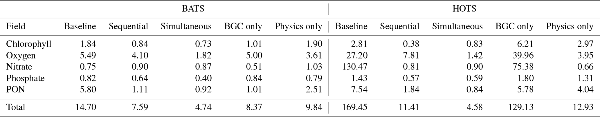
Figure 3c–f provide results for each of the parameter estimations at BATS. Figure 3c and Table 3 show that the calibrated case that only includes the 12 most sensitive BGC parameters was unable to significantly improve agreement with the observational data for BATS, compared to the baseline model. Similarly, only estimating the physical parameters (as the first calibration in the sequential study) produced only moderate improvements. A comparison of fields across the calibration cases (Fig. 3e–f) demonstrates that the simultaneous optimization of the physical and BGC parameters produces the best results, with each of the variable fields generally in better agreement with the observational data in the simultaneous estimation case. Nitrate is an exception, where the optimized results under-predict the observed concentrations at the bottom boundary. This tendency is also evident in the normalized RMSD values calculated for each of the target fields.

The results of the BGC only and sequential calibration cases were similar in overall agreement, and sequential calibration outperformed the previous two calibration methods. The field-specific normalized RMSD values show that better agreement is obtained for phytoplankton chlorophyll, oxygen, and phosphate. Improvements in chlorophyll and oxygen can also be clearly observed in the field results.

The coefficients for the vertical eddy velocities are an important component of the parameter estimation. Figure 4 shows the complete vertical velocity profiles of the baseline parameterization of mesoscale eddies. Figure 4a shows the velocity profiles applied to the first 15 d of each month, and Fig. 4b shows the profiles for the second 15 d. Figure 4c shows the full time series using the maximum velocity of each profile, which is always located at the bottom of the water column. The estimated results are shown in Fig. 4c using a moving average to show the trend in the velocities throughout the year.

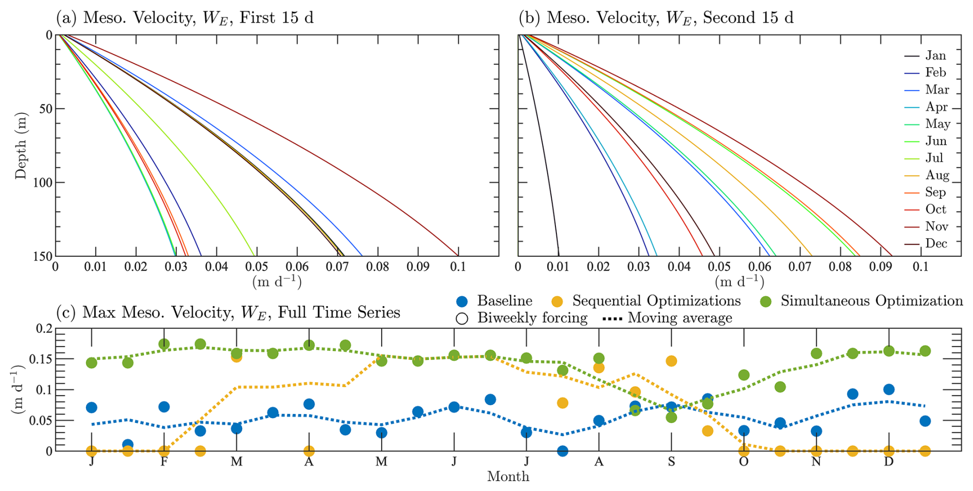
Figure 4 Parameterization of vertical velocity profiles from mesoscale eddies for the BATS location. Panels (a) and (b) are the full semi-monthly velocity profiles applied to the first and second halves of each month, respectively. The profiles correspond to the baseline case. In panel (c), the maximum velocity values are shown throughout the annual cycle, including data from the baseline case, the sequential calibration, and the simultaneous calibration.

Figure 4c shows that the baseline parameterization is randomly distributed between 0 and 0.1 m d⁻¹ throughout the year. There is a slight shift towards higher velocities at the end of the year after August. As a result of relaxing the upper limit to  0.2 m d⁻¹, both the sequentially and simultaneously calibrated velocity profiles produce higher velocities, but with different trends. The sequential calibration case increases vertical velocities from March through the end of August. From October through February, the velocities are estimated to be 0 m d⁻¹.

The simultaneous estimation produces a more reasonable annual cycle in vertical velocities, contributing to better agreement with the observational values at BATS. Vertical mesoscale velocities are predicted to be higher for most of the year than in the baseline case, but with a clear decrease in vertical velocities from July through the end of October. These trends match expectations, since there is more vertical transport associated with mesoscale eddies (Mahadevan and Archer, 2000; Salmon et al., 2015) during the fall and winter when the eddies are more abundant (Aguedjou et al., 2019).

4.2 Hawaii ocean time-series (HOTS)

As with the BATS site, we show all observational and model data for the HOTS site in Fig. 5. The HOTS annual cycle has a similar pattern to that of BATS but with smaller seasonal changes, as shown in Fig. 5a. Phytoplankton chlorophyll has a persistent subsurface maximum at 100 m depth, with higher concentrations from October through February. There are also increased concentrations below 100 m from March through July. There is a slight decrease in oxygen concentrations near the surface from May through November, but the overall variation in concentration is relatively low. Nitrate and phosphate are confined to the bottom of the domain. They have increased vertical transport from November through February with additional upwelling events; the first is May through June for nitrate and April to May for phosphate, and the second is August to September for both. The PON is primarily in the upper portion of the domain. There is a slight increase in concentration from March through October between 25 and 75 m.

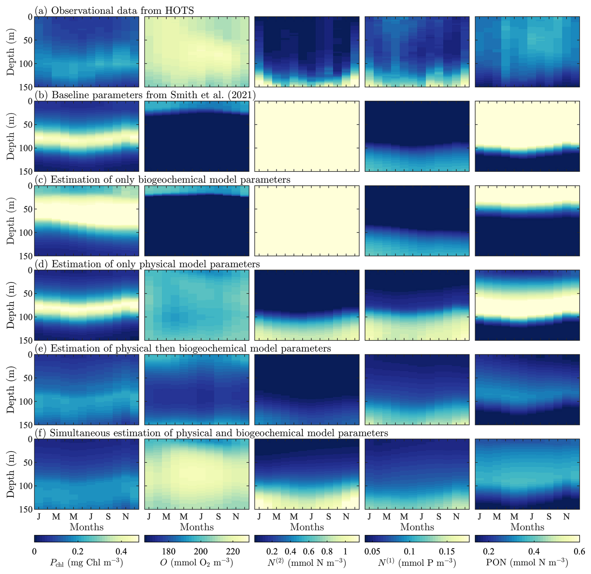
Figure 5 HOTS observational and model results for target-field concentration data for (from left-to-right) phytoplankton chlorophyll (P_chl), oxygen (O), nitrate (N⁽²⁾), phosphate (N⁽¹⁾), and particulate organic nitrogen (PON). Row (a) is the reference observational data and subsequent rows correspond to model runs with the parameter values from Smith et al. (2021) (b), estimated BGC parameters only (c), estimated parameters in the physical model only (d), sequentially estimated parameters (e), and simultaneously estimated parameters (f).

Compared to the BATS site in Fig. 3, the results of the baseline model shown in Fig. 5b for HOTS diverge significantly from the observational data. However, it is important to note that the baseline parameter values used by Smith et al. (2021) were initially taken from a 56-state variable implementation of BFM for coastal locations. Some of the BGC and boundary control parameters in the baseline model were also manually tuned by Smith et al. (2021) specifically for the BATS site. As a result, it is not surprising that the observational and baseline model results do not match well for the HOTS location, since the baseline BFM17 parameters were not adjusted for this BGC community.

The baseline results in Fig. 5b show that the modeled phytoplankton, nitrate, phosphate, and PON have annual cycles similar to the observations, but the concentration magnitudes and community structure are poorly predicted. Phytoplankton chlorophyll is over-predicted throughout the year and the subsurface maximum is not as deep in the water column as the observational data, being closer to 75 m than the observed 100 m. Nitrate is severely over-predicted, while phosphate is under-predicted to a lesser degree. PON is severely over-predicted and does not extend as deep into the water column as in the observational data. The most significant differences are between the observational and simulated oxygen fields. Neither the annual cycle nor the concentrations are close to those in the observational data.

By comparing the observational and baseline model results for BATS and HOTS, we observe similarities in the trends in the observed and predicted annual cycles of the target fields. This suggests that BFM17 + POM1D is capable of successfully representing the target BGC communities. However, there are significant differences, which implies that the model requires tuning to successfully represent a biogeochemical community. In Kern et al. (2024), the complete set of BGC parameters in BFM17 was optimized to improve the model results, both individually and simultaneously at BATS and HOTS. Considerable improvements in the model agreement were obtained for HOTS in particular. In the present study, we examine whether we can improve the fit of the model to the mean seasonal cycle by simultaneously estimating key physical and BGC parameters. Simultaneous physical and BGC parameter estimation should produce more realistic BGC and physical parameter estimates than sequential physical-BGC parameter estimation, which can produce BGC parameter estimates that compensate for biases in physical parameter estimates, and vice versa.

At the HOTS location, Fig. 5 and Table 3 show that the calibrated case only including the 12 most sensitive BGC parameters was unable to significantly improve agreement with the observational data. However, in this case, there are significant improvements compared to the BATS case for the estimation of the physical parameters only, which is followed by moderately improved agreement from the subsequent calibration of the BGC model parameters. It is interesting to note that, at HOTS, the oxygen results agree less well with the observational data after the sequential calibration of the BGC parameters, as compared to the physical model calibration only. This decrease in the accuracy of the oxygen prediction is also present – but less pronounced – at BATS. At HOTS, the reduced agreement in oxygen is offset by improved agreement for nearly every other field, particularly phytoplankton chlorophyll and PON. This type of outcome is generally unsurprising in an optimization framework where multiple fields are combined into a single objective function; provided that the overall objective function value is lower, as is the case after the sequential optimization, the calibrated parameter set is more successful overall. It is possible that if certain variables, such as the boundary relaxation for oxygen, were instead included in the set of BGC parameters, this effect would be less pronounced. However, we would still expect there to be a lower total objective function value for the sequential case than the physical-model-only case.

Despite an overall improvement in the sequential calibration case, the best agreement was achieved by simultaneously optimizing the BGC and the physical model parameters, as at the BATS location. All five variable fields show improved results, reproducing the annual cycle. The phytoplankton chlorophyll and nitrate are still over-predicted in some portions of the water column and the PON has a subsurface maximum near 100 m instead of the observed 25–50 m, but in all cases the normalized RMSD has decreased. With the exception of phytoplankton, all simultaneous calibration results are at least on par with those of the sequential calibration methodology. The simultaneous calibration case ultimately performs best by getting significantly better results in oxygen (with a normalized RMSD of 1.42 compared to 7.81, as shown in Table 3) and PON (0.84 compared to 1.84), resulting in a total normalized RMSD of 4.58 compared to 11.41.

Figure 6 shows the annual variability in mesoscale eddy vertical velocity profiles for the baseline, sequential calibration, and simultaneous calibration cases, following the format of Fig. 4. The baseline case set the vertical eddy velocities very low, with the majority less than 0.05 m d⁻¹. The values are especially low from January to March, after which they start to increase, with the largest values occurring in August and September. The sequential calibration increases velocities throughout the year, while driving some values to 0 m d⁻¹, especially from mid-January through the beginning of April. The variability predicted by the simultaneous calibration case shows that vertical velocities throughout the year are higher, with a majority of values between 0.15 and 0.2 m d⁻¹. Although confirmation of the seasonal variability in vertical transport by mesoscale eddies at HOTS requires further validation in the future, the results are similar to the annual cycle observed at BATS, with some differences in the timing and degree of seasonal variation. We also note that the estimated vertical settling velocity at HOTS is higher than at BATS (1.5 m d⁻¹ vs. 0.5 m d⁻¹, respectively).

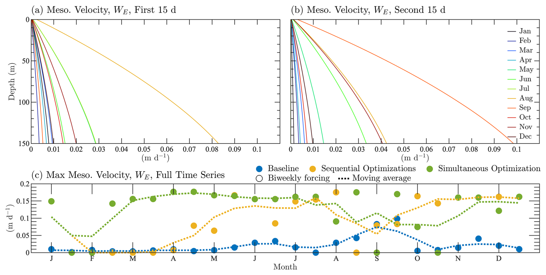
Figure 6 Parameterization for vertical velocity profiles from mesoscale eddies for the HOTS location. Panels (a) and (b) are the full semi-monthly velocity profiles applied to the first and second hafts of each month, respectively. The profiles correspond to the baseline case. In panel (c), the trend in vertical velocity profiles is shown using the maximum velocity throughout the annual cycle, including data from the baseline case, the sequential calibration, and the simultaneous calibration.

Finally, consistent with the findings in Kern et al. (2024), there are differences in the estimated parameters at the BATS and HOTS locations (see Table C2 for the final parameter values). This suggests that global BGC models may benefit from allowing for spatial variation in the model behavior across distinct BGC communities. However, this variability is also dependent, in part, on the model being used. In the present study, we are using a moderately complex model with phytoplankton and zooplankton species that represent community average behaviors. With more specificity, the model parameters could require less variability across regions.

5 Conclusions

We have estimated parameter values for the coupled BGC and physical model BFM17 + POM1D using a multi-step automatic methodology that was previously developed in Kern et al. (2024) to efficiently tune a large number of model parameters. Our objective in this study has been to find a methodology for estimating the parameters that will most accurately represent the observed data from target BGC fields. We found that it was necessary to include the estimation of the advection, boundary condition, and turbulent diffusion parameters present in the physical model to get the best agreement with the target fields. The cases we have performed address questions about how to efficiently and effectively incorporate parameter sets from multiple components of a biophysical model into a single parameter estimation.

In our study, we examine for the first time the best approach to apply the parameter estimation methodology to multiple components of a coupled biophysical model in a 1D environment. We tested two approaches: the first was to sequentially calibrate the advection, boundary condition, and turbulent diffusion parameters and then the exclusively BGC parameters. It should be noted that this approach could also be applied in an iterative framework where, after estimating both sets of parameters, the entire sequential estimation procedure would be repeated. Here, we have performed the first iteration of such a process.

The second approach examined here involved the simultaneous estimation of BGC parameters and the parameters associated with other model components. For the BATS location, the simultaneous estimation outperformed the sequential estimation for all target fields. The general disagreement between the model results and observational data was 30 % less in the simultaneous estimation than in the sequential estimation. For the HOTS location, the overall model performance was much better after the simultaneous estimation than in the sequential case. The overall disagreement from the sequential results was more than a factor of two higher than the simultaneous results, due in part to a reduction in the accuracy of the oxygen results from the estimation based on the physical model parameters only to the sequential optimization.

An important outcome of the parameter estimation studies was more realistic behavior in the vertical eddy velocities. The simultaneous parameter estimation for BATS produced an annual cycle in vertical eddy velocities that was more realistic. Similarly, the simultaneous parameter estimation for HOTS produces a more reasonable cycle. However, in the latter case, there was decreased activity later in the year. We also found variability in the calibrated values of the parameters at BATS and HOTS, for example in the vertical settling velocity, suggesting that location dependent variability in the model parameters could allow greater applicability of the resulting models across different ocean locations.

It is important to clarify that the need to simultaneously calibrate the various components of the biophysical model arises from the specific formulation of the physical model and parameterizations in POM1D. The model has imposed temperature and salinity profiles from the observational time series, while vertical velocities are imposed from a parameterization assuming a general circulation profile based on wind stress values and an assumed Ekman depth. The mesoscale eddy velocities are semi-monthly perturbed versions of the monthly general circulation profiles. We only have observational BGC data to perform the estimation, which necessitates the simultaneous estimation of both model components. In other contexts, where there are passive tracers that can be used to estimate the physical model separately from the BGC model, it could be practical and beneficial to calibrate the physical model first and subsequently the BGC model. Temperature and salinity can also be solved prognostically, if these variables are not imposed from observational data as in the present tests. Generally, 3D models can be configured to allow for the physical and BGC models to be calibrated independently, which would likely make the BGC parameter calibration converge faster.

The present methodology can also be extended to 3D cases where the entire water column is modeled and relaxation coefficients are not needed at the bottom boundary. However, the overall computational cost of the parameter estimation will increase considerably due to the higher dimensionality of the simulations, potentially restricting the number of parameters that can be estimated. Nevertheless, it is likely that even when using a benthic return or a settling velocity at the bottom boundary, the associated control parameters will need to be estimated along with the BGC parameters. In addition, the applicability of the present models – which have parameter values estimated using 1D cases – in 3D physical scenarios remains an open question. As a result, caution is recommended when using the estimated values in contexts beyond the 1D BATS and HOTS scenarios presented here. We also note that for ocean locations where there are only a few observations, the present methodology could still be used. However, care would have to be taken in applying the resulting models to new scenarios, since the parameter estimation would have been based on only limited information.

Although this study specifically examines the best way to incorporate different model components into a single calibration, it also serves as a demonstration of a meta-algorithm for performing calibrations of high-dimensional models using a truncated global search with local optimizations. In Kern et al. (2024), we addressed the problem by developing a methodology, summarized in Sect. 2, capable of estimating the full set of BGC parameters. In this study, we include a similar number of parameters, but not all of the BGC parameters. As a result, the meta-algorithm demonstrated can be summarized as:

1. Test model sensitivity to input parameters;

2. Select parameters for estimation;

3. Probe the reduced parameter space;

4. Perform local optimizations from the best performing parameter sets;

5. Select the best performing optimized parameter set as the final solution.

The particular methodology applied in this paper is a specific implementation of this general framework. For model sensitivity, we perform one-at-a-time parameter perturbations. We then select the parameters that are most sensitive for different observational time series. We probed the parameter spacing using randomly generated parameter sets with a Latin hybercube sampling algorithm from DAKOTA. Finally, we use a quasi-Newton algorithm from the Opt$++$ library in DAKOTA to perform local optimizations and select the best parameter set from their results.

The results of the parameter estimation will depend on the available data, the objective function formulation, the model location, and the analysis methods used. Although the methods applied here have been shown to work well for the present parameter estimations, all can be changed to fit the problem being addressed, the needs of the user, and the available computational resources. As stated in Sect. 2, this methodology cannot guarantee that the global minimum has been found. However, the global search and multi-start approach will increase the exploration of the parameter space and decrease the impact of user-selected parameter sets. The calibration can also only be expected to improve the overall agreement across observational fields included in the objective function. Depending on the community structure, model, and target outputs, improvements in state variables unaccounted for in the objective function can happen, but should not be expected as a principle. For each implementation of this methodology, an appropriate objective function must be formulated based on the application and purpose of the biophysical model.

Future work is also required to examine the potential issues with overfitting, where the use of optimization techniques may drive parameters to unrealistic or unrepresentative values to achieve artificially low error. As noted previously, the general framework applied here is flexible, so more sophisticated techniques may be applied, including regularization before optimization (Ghojogh and Crowley, 2023) or statistical parameter selection approaches like Bayesian estimation. Another concern worth further exploration is the identification and leveraging of correlated parameters. In the methodology applied here, we used a common but relatively simple approach to sensitivity analysis. Using more sophisticated methods for dimension reduction, like active subspace analysis (Ji et al., 2018), during the parameter selection step could address this challenge. Finally, other optimization approaches such as simulated annealing and genetic algorithms are worth exploring in the future.

Appendix A: Biogeochemical Parameter Selection

Kern et al. (2024) primarily focused on estimating parameters in the BGC model. Here, we also estimate 30 parameters from the physical model, a majority of which were not previously considered. The parameters included from the physical model are 1 turbulent mixing parameter, 1 sinking velocity, 4 boundary control parameters, and 24 coefficients for the vertical eddy velocity profiles. The sinking velocity and boundary control parameters were included by Kern et al. (2024), but here they are included specifically as part of the physical model. Since there are already 30 identified physical model parameters to be estimated, we opted to reduce the full set of 46 BGC parameters in BFM17 to manage the computational requirements of the estimation problem.

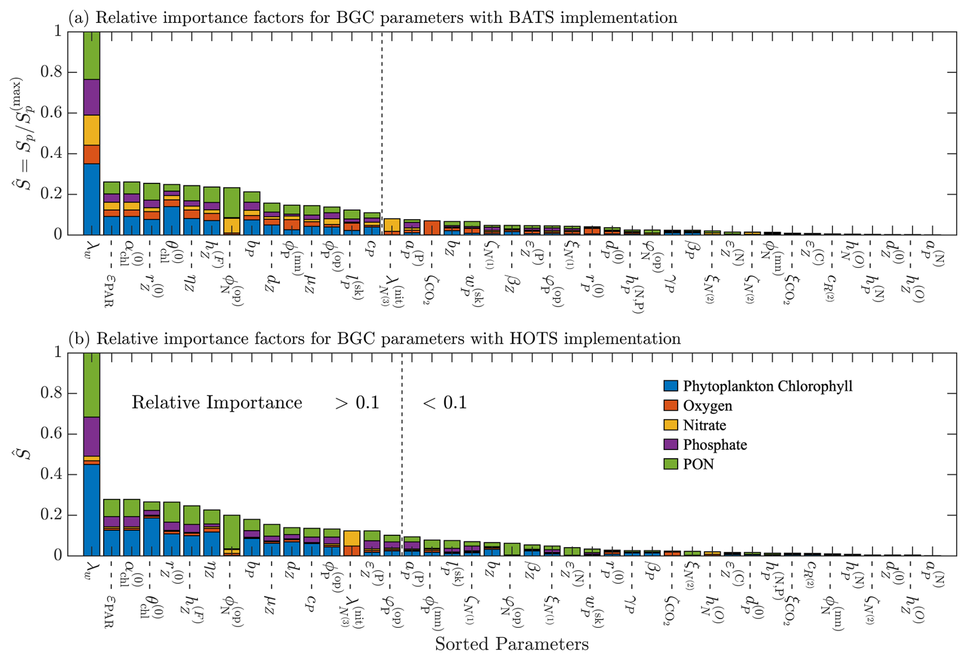
Figure A1 Results of a one-at-a-time sensitivity study performed for the BATS (a) and HOTS (b) locations. The parameters are ranked based on their relative importance for each location, with the values shown on the bar plot. A dotted line is included on both plots to indicate where the relative importance values fall below 0.1.

The greater the number of parameters, the more complex the objective function space. This is an important consideration, as the parameter estimation methodology implemented here employs gradient-based optimization. For gradient-based optimization, we have to estimate the gradient in each dimension in the objective function space. Each additional parameter introduces a dimension along which we have to approximate the gradient with finite differencing, requiring two more model evaluations. Also, the more complex the objective space, the easier it is to fail to converge to a solution or to converge to a poorly performing local minimum. We therefore reduce the set of BGC parameters; the resulting parameter set is still sufficient to allow a comparison of sequential versus simultaneous optimization of BGC and physical models, which is the primary focus of the present study.

To reduce the set of parameters to be estimated in the BGC model, we performed a one-at-a-time sensitivity study to determine the relative sensitivity of BFM17 to each parameter. Each parameter is independently perturbed by 5 % from its baseline value. The model is tested with a positive and negative perturbation, except where the perturbed value exceeds the upper or lower bound of the parameter range. The baseline parameter values and parameter limits are provided in Table 1 for those ultimately selected for the estimation study and in Table C1 for those excluded. The objective function, defined in Eq. (1), is calculated for each perturbed case, with the maximum of the positively and negatively perturbed cases taken as the sensitivity metric, S_p, for each parameter. The parameters are compared using a relative importance, ${\widehat{S}}_{\mathrm{p}}$, defined as

$$\begin{array}{}\text{(A1)}& {\widehat{S}}_{\mathrm{p}}=S_{\mathrm{p}}/S_{\mathrm{p}}^{\left(\max \right)},\end{array}$$

where $S_{\mathrm{p}}^{\left(\max \right)}$ is the maximum sensitivity factor across parameters for a given location.

The results of the sensitivity analysis are shown in Fig. A1 for the BATS and HOTS locations. Relative sensitivities are shown for each parameter, with the parameters ordered according to relative importance values (from highest to lowest). Figure A1 compares the contribution of each target field to the final relative importance metric, as indicated by the portion of the total normalized differences that come from each field. The most important parameters are those with the highest relative importance values. We separated the parameters into two groups using a threshold of ${\widehat{S}}_{\mathrm{p}}=\mathrm{0.1}$, which is indicated in Fig. A1 by dashed lines, with the parameters on the left having relative importance greater than the threshold and the parameters on the right less than the threshold. The 0.1 threshold is used in this study because we would like no more than 20 additional BGC parameters to keep the total number of parameters estimated similar to the number included in Kern et al. (2024). Furthermore, the twin simulation studies presented by Kern et al. (2024) suggest that we should be able to recover parameters with relative importance values greater than 0.01 for BFM17 + POM1D. Our threshold of 0.1 is therefore conservative. Ultimately, fifteen parameters met the threshold condition for BATS, while 16 parameters met the condition for HOTS. We chose to use the minimum number of common parameters between the two locations (i.e., the intersection set) since we would like to optimize a consistent set of parameters for both locations and the intersection set includes most of the important parameters at each location.

In total, there are 13 parameters in the intersection set, of which 12 will be used in our estimation studies. The selected parameters are presented in Table 1. The zooplankton feeding threshold, μ_Z, also met the criteria to be included in the estimation study. However, since the parameterization of zooplankton production (Smith et al., 2021, Eq. (A34)) uses the potential specific growth rate ($r_{\mathrm{Z}}^{\left(\mathrm{0}\right)}$), the Michaelis constant for total food ingestion ($h_{\mathrm{Z}}^{\left(\mathrm{F}\right)}$), and the feeding threshold (μ_Z), only the two most important of the three parameters (as expressed by the relative importance) are retained for subsequent calibration studies.

Appendix B: Twin Simulation Experiments

Before proceeding with the parameter estimation studies, the methodology and its implementation were tested using a Twin Simulation Experiment (TSE), as in Spitz et al. (1998), Athias et al. (2000), Kidston et al. (2011), Oliver et al. (2022), and Kern et al. (2024). In a TSE, we attempt to recover the values of known parameters from a perturbed initial state. The target data are synthetic and generated using the model with the baseline parameter values. The TSE presented here was performed for the BATS location using the 12 selected BGC parameters from the previous section. Using the perturbed initial values, we tested whether the applied method was able to correctly predict the baseline parameter values. The TSE parameters and their target values (i.e., the baseline values) are included in Table 1.

The initial parameter values were set by increasing the baseline parameter values by 10 %, consistent with the tests performed by Kern et al. (2024). We then applied the parameter estimation methodology to recover the baseline values, giving the results shown in Fig. B1, where we calculate the difference between the normalized parameter value tested, ${\widehat{p}}_{\mathrm{i}}$, and the normalized baseline parameter value, ${\widehat{p}}_{\mathrm{0}}$, for each parameter. The parameter values are normalized to a domain between 0 and 1 using the lower and upper limits included in the final column of Table 1.

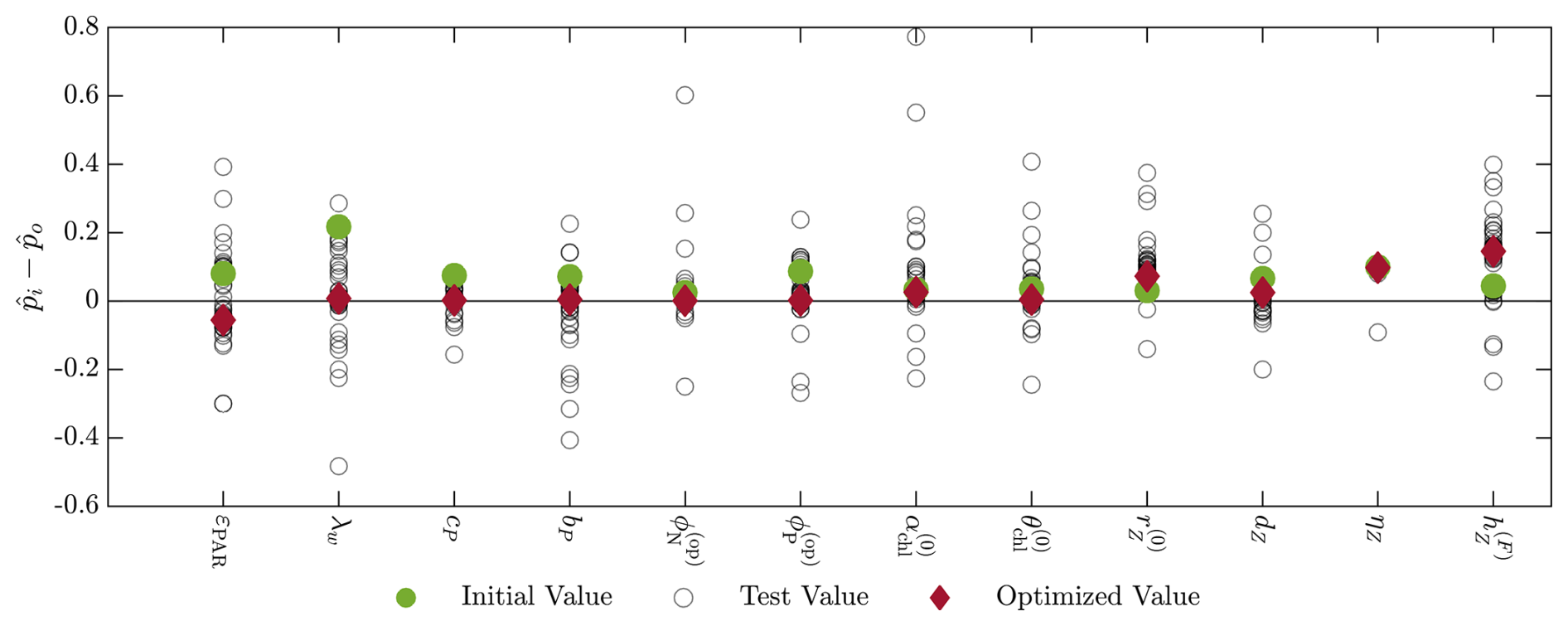
Figure B1 Results of the twin simulation experiment with the 12 selected BGC parameters included in the parameter estimation study. The initial values (green dot), final value (red diamond), and intermediate test values (empty circles) are shown as the difference between the normalized parameter value (${\widehat{p}}_{\mathrm{i}}$) and the normalized nominal parameter value (${\widehat{p}}_{\mathrm{o}}$). The normalization is between 0 and 1 based on the upper and lower bounds of the parameter value ranges presented in Table 1.

Figure B1 shows that the estimated parameter values are all close to the baseline values. Of the 12 parameters tested, 9 have moved towards the baseline value, while 1 does not change. As noted in Appendix A, the remaining two parameters, $r_{\mathrm{Z}}^{\left(\mathrm{0}\right)}$ and $h_{\mathrm{Z}}^{\left(\mathrm{F}\right)}$, appear in the same zooplankton equation in the BGC model, along with the feeding threshold μ_Z. When using all three parameters in the TSE, the method was unable to recover the baseline values for any of the parameters, but did perform better when using only two of the parameters. Although the method moves in the direction of the baseline values for these parameters, the parameters are still able to adjust to compensate for each other because they appear in the same governing equation.

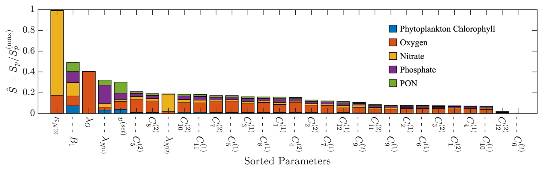
Figure B2 Results of a one-at-a-time sensitivity study performed for the BATS location. The parameters are ranked based on their relative importance, with the values shown on the bar plot.

The results of the TSE indicate that the parameter estimation methodology can be successfully applied to the model to improve the agreement with the target data. The results of the TSE also confirm that the optimization toolbox and the model have been correctly connected to each other. Most importantly, the results indicate that we have selected a reasonable set of parameters from the BGC model to proceed with the rest of the study.

To assess the calibration capabilities of the optimization algorithm beyond the BGC parameters, an additional TSE was performed. To start, the most sensitive parameters among the advection, boundary condition, and turbulent diffusion parameters for the BATS site were determined using a one-at-a-time sensitivity analysis. The five most sensitive parameters were then selected for the additional TSE, which ultimately included 17 parameters from both the BGC and other model components. The TSE was conducted following the same procedure as described above.

Starting with the sensitivity analysis, the additional results are included in Fig. B2. The 5 most sensitive parameters are the relaxation diffusivity for ammonium (${\mathit{\kappa }}_{{\mathrm{N}}^{\left(\mathrm{3}\right)}}$), the stability function coefficient (B₁), the relaxation constant for oxygen (λ_O), the relaxation constant for phosphate (${\mathit{\lambda }}_{{\mathrm{N}}^{\left(\mathrm{1}\right)}}$), and the settling velocity of particulate detritus (v^(set)). The sensitivities have been normalized by the max sensitivity factor in the present study, where we note that the maximum raw sensitivity factor for the BGC parameter sensitivity in Appendix A was larger than the maximum from the physical parameter sensitivity analysis. The listed five parameters were selected to be included in the additional TSE. It is interesting to note that the coefficients for the semi-monthly mesoscale eddy profiles were relatively insensitive in Fig. B2, although most had the greatest sensitivity for the oxygen state variable.

The results of the 17-parameter TSE are presented in Fig. B3. The results demonstrate that we tend towards the baseline parameter values in most cases. Notably, the results for the exclusively BGC parameters are consistent between the two tests, which is reasonable considering the higher sensitivity to those parameters. Yet, the settling velocity tends toward the baseline parameter value, while the relaxation coefficients remain in the proximity of their baseline values. The stability function parameter remains at its initially guessed value, due to the fact that the perturbed value also provides a satisfactory result, combined with its relatively narrow bounds compared to some other parameters.

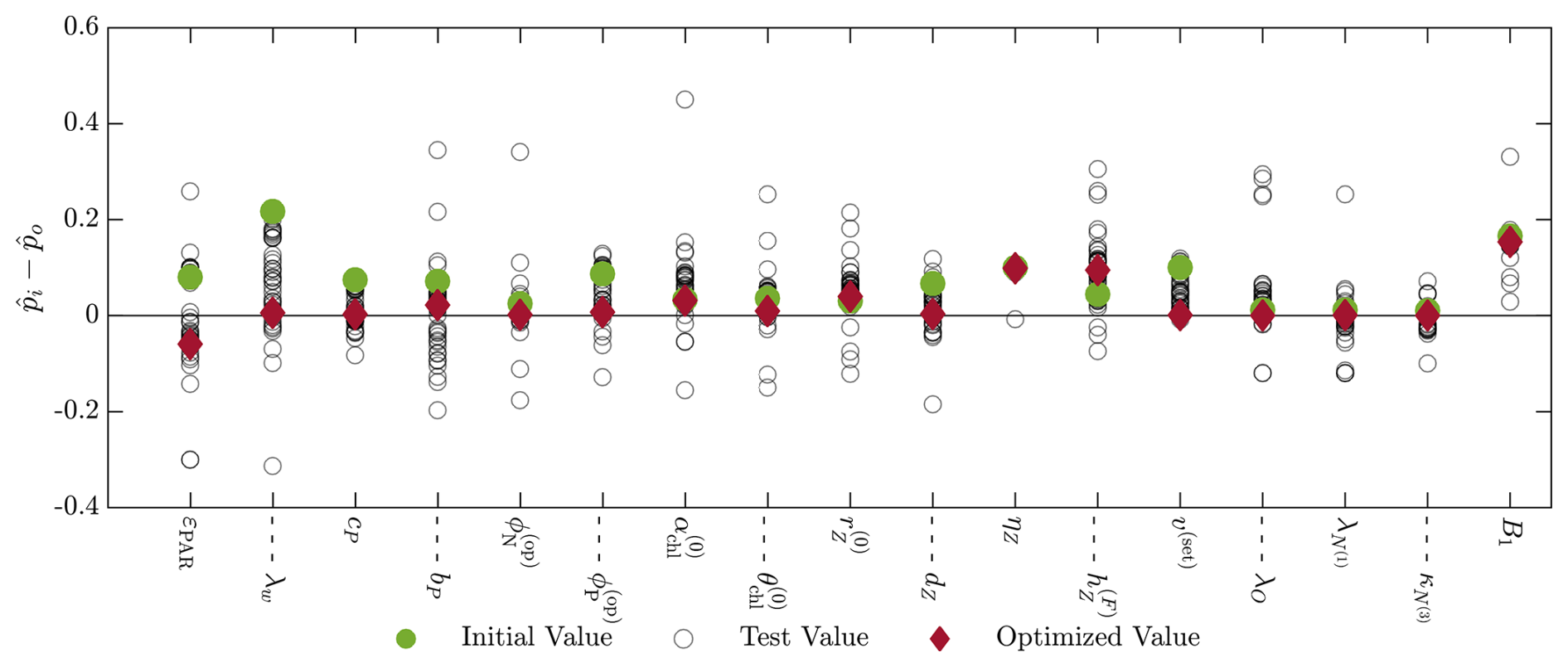
Figure B3 Results of the twin simulation experiment with the 17 parameters including the BGC, advection, boundary condition, and turbulent diffusion parameters. The initial values (green dot), final value (red diamond), and intermediate test values (empty circles) are shown as the difference between the normalized parameter value (${\widehat{p}}_{\mathrm{i}}$) and the normalized nominal parameter value (${\widehat{p}}_{\mathrm{o}}$). The normalization is between 0 and 1 based on the upper and lower bounds of the parameter value ranges presented in Table 1.

These results allow us to proceed to the parameter calibration runs included in the paper. While the TSE results in Fig. B3 did not include the coefficients for the semi-monthly mesoscale eddy profiles, those were ultimately included in the final runs. Although these coefficients were relatively insensitive for the baseline values about which the present sensitivity analysis was performed, the truncated global search in the full parameter estimation methodology allows for a much broader search of the parameter space, for which it is appropriate to include these coefficients in the estimation.

Appendix C: Additional Tables

Table C1 List of values for BFM17 parameters not included in the calibration.

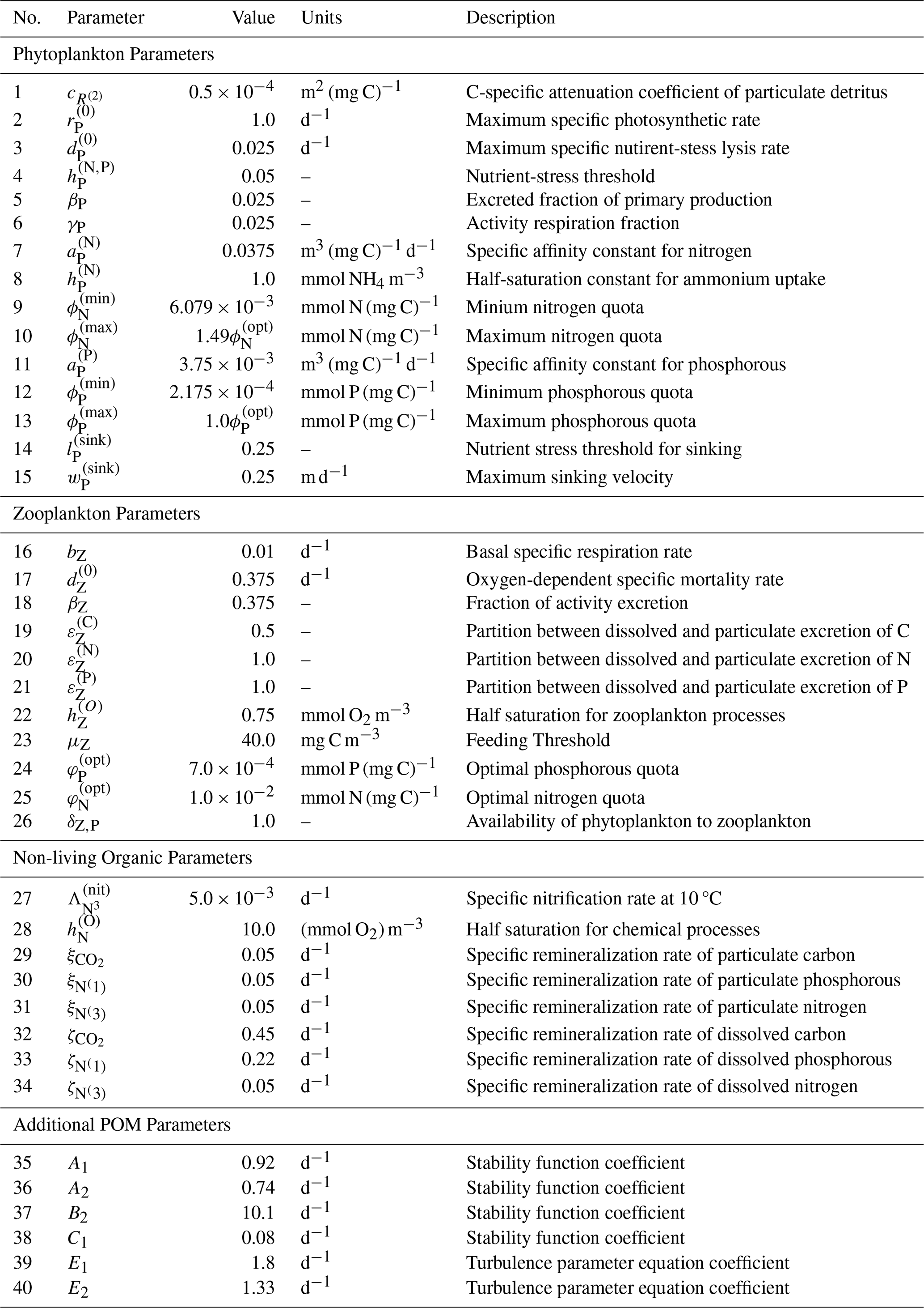
Table C2 List of calibrated model parameters and coefficients for BATS and HOTS locations. If the bounds vary between cases which is only true for the velocity coefficients, the HOTS parameter is in parenthesis.