Veris: fast & efficient sea-ice modeling in Python with GPU acceleration

Climate models have traditionally been developed in Fortran, due to its long-standing use in scientific computing and its excellent computational performance. While Python offers substantial advantages in terms of code readability, maintainability, and the availability of libraries and tools, the performance gap between Python and Fortran has historically limited Python's use in large-scale climate modeling. This performance gap can be mitigated by using the JAX library, which significantly improves execution speed of Python code.

We use JAX as a backend for Veris, a new sea ice model implemented in Python. Veris builds upon the Fortran-based sea ice component of the general circulation model MITgcm. Benchmark experiments show that Veris exhibits scaling behavior with increasing process counts comparable to the Fortran reference implementation. For small CPU process counts, Veris outperforms the MITgcm, showing the great potential that JAX has for climate modeling, particularly as further improvements in inter-process communication are anticipated. When executed on a high-end GPU, a single-process Veris simulation matches the performance of the parallelized Fortran reference running on hundreds of CPU cores, but at a fraction of the energy cost. These results demonstrate the potential of Veris for large-scale HPC-based simulations.

1 Introduction

Climate models contain hundreds of thousands of lines of code. The programming language used in these models is typically Fortran, largely due to its legacy in scientific computing. Fortran's strong backward compatibility allows extensive reuse of existing code in newer models written in updated versions of the language, saving significant development time compared to rewriting legacy code in a different language. Another key reason for Fortran's prevalence is its high computational efficiency in compute-intensive climate models (Méndez et al., 2014). While numerical computation speed was historically the primary bottleneck, modern hardware has shifted this limitation to memory bandwidth. Fortran allows for low-level optimizations, such as SIMD (Single Instruction Multiple Data) vectorization and direct memory addressing, critical for performance in bandwidth-bound climate simulations (Rasmussen et al., 2024).

Despite these advantages, Fortran is relatively unpopular compared to modern languages like Python, especially among scientists outside climate modeling. This can create a barrier for new researchers, who have to invest substantial time in learning an unfamiliar programming language. Additionally, using a more popular language such as Python would enable access to more libraries and tools. Fortran, though well-suited for high-performance computing (HPC) due to its optimization for numerical and array-based calculations, can be more challenging to work with than higher-level languages. Using a high-level language such as Python would not only facilitate structural modifications, such as implementing new parameterizations and subsequent debugging, but would also make HPC workflows more accessible to researchers who may lack extensive experience in low-level programming.

Although Python's popularity and readability offer advantages, these factors alone do not justify switching from Fortran to Python due to the significant performance gap between the two languages without optimizations or extensions. To overcome this gap, the Python library JAX can be used to significantly increase Python's performance for numerical modeling (Bradbury et al., 2018). JAX is a library for array-based computing with a syntax very similar to NumPy's (Harris et al., 2020), allowing NumPy code to be adapted to JAX without structural changes. JAX includes a set of function transformations like vectorization, parallelization, automatic differentiation and Just-In-Time (JIT) compilation. The JIT compilation significantly reduces the runtime of iterative calculations, making JAX well-suited for climate models as they iterate over many time steps.

In addition to these transformations, a key advantage of JAX is that it is agnostic to the type of accelerator, enabling the same code to run on both CPUs and GPUs. Due to their higher core counts, GPUs are much better suited for parallel computing than CPUs, provided that the available computational and memory resources are fully utilized. As a result, they are more energy-efficient for parallel tasks such as climate simulations, as they complete these simulations faster than CPUs. By leveraging GPUs, JAX not only enhances computational speed but also reduces the power consumption and therefore the carbon footprint of running climate models (e.g., Marquetti et al., 2018; Portegies Zwart, 2020; Li et al., 2023). Unfortunately, many climate models cannot fully utilize state-of-the-art hardware, motivating the development of models with efficient GPU support.

One example is the Python based Versatile Ocean Simulator (Veros, Häfner et al., 2018, https://veros.readthedocs.io/en/latest/, last access: 1 June 2026), which is a translation of the Fortran backend of the ocean model pyOM2 (v2.1.0, Eden and Olbers, 2014; Eden, 2016). By using the Just-In-Time compilation of JAX, the performance gap to the original Fortran model was closed (Häfner et al., 2021). When using JAX as the backend, Veros can be run on both CPUs and GPUs. With a single GPU, dozens to hundreds of CPU cores can be replaced which substantially reduces the energy consumption of running Veros.

To date, Veros does not contain a sea ice model, limiting its applicability in high-latitude regions where sea ice significantly influences heat, momentum, and moisture exchanges between the ocean and atmosphere, thereby impacting the local climate. This work introduces Veris (Versatile Sea Ice Simulator), a Python-based sea ice model originally developed to be coupled to Veros to extend its range of applications. Like Veros, Veris supports both NumPy and JAX backends. When used with JAX, Veris can also run on GPU architectures, providing substantial computational advantages. In order to parallelize Veris, the model infrastructure was subsequently redesigned, resulting in a separate, updated version of Veris that is able to leverage JAX's parallelization capabilities on both CPU- and GPU-based systems. Owing to these architectural changes, this parallelized version is no longer directly compatible with Veros, but instead represents an independent, high-performance sea ice modeling framework optimized for large-scale simulations.

To solve the momentum equation, Veris employs the modified and adaptive elastic-viscous-plastic (EVP) solver (Lemieux et al., 2012; Bouillon et al., 2013; Kimmritz et al., 2015, 2016). Benchmark experiments by Rasmussen et al. (2024) assessed a refactored implementation of the standard EVP solver used in the Fortran-based sea ice model CICE (Hunke et al., 2024), optimized for parallel execution on both CPU- and GPU-based architectures. In these experiments, execution on a single GPU was found to be 1.2 times faster than on 112 CPU cores. Accordingly, a significant performance increase is anticipated for Veris when comparing GPU-based execution to CPU-based configurations.

The properties of Veris are described in Sect. 2. Section 3 presents benchmark simulations to verify that Veris accurately simulates sea ice dynamics, as well as performance benchmarks comparing Veris to the Fortran reference.

2 Model Description

2.1 Basic Properties

Veris is a Fortran to Python translation of part of the sea ice component of the Massachusetts Institute of Technology general circulation model (MITgcm, Marshall et al., 1997; Losch et al., 2010, https://github.com/MITgcm/MITgcm, https://mitgcm.org/documentation/, last access: 1 June 2026), originally based on the formulation by Hibler (1979). The core properties of Veris are as follows:

• The variables are stored on a two-dimensional, staggered C-grid (Arakawa and Lamb, 1977). Tracer variables, such as ice thickness and concentration, are stored at the centers of grid cells, while the u- and v-components of velocity are stored at the respective u- and v-grid points.

• Ice grows thermodynamically when the ocean loses heat to the atmosphere through a conductive heat flux across the ice. This heat loss is balanced by freezing at the ice bottom. Additionally, new ice may form in regions of open water when the ocean is loosing heat. For the growth rate calculation, a two level thickness configuration is assumed (Hibler, 1979). Each grid cell is assumed to contain ice of thickness h_actual and open water. The proportion of the grid cell that is covered with ice is defined as the ice concentration A. The actual ice thickness h_actual is derived from the mean ice thickness per grid cell h according to $h_{\mathrm{actual}}=\frac{h}{A}$. The growth of the mean thickness over a single time step is

  $$\begin{array}{}\text{(1)}& \mathrm{\Delta }h=\mathrm{\Delta }t\left(f\right(h_{\mathrm{actual}})A+f(\mathrm{0}\left)\right(\mathrm{1}-A)+f_{\mathrm{ml}})\end{array}$$

  where f(h) is the growth rate of ice of thickness h, and f_ml accounts for ice melting at the base due to the mixed layer temperature.

• The ice has no heat capacity, and the adjustment of the ice surface temperature to changes in the surrounding temperature occurs instantaneously (zero-layer thermodynamics, Semtner, 1976).

• Snow can accumulate on the ice cover under conditions of snowfall or freezing rain.

• Additional ice growth can occur if the weight of accumulated snow submerges the ice. When the ice-snow interface lies below the water surface, a simple mass conserving parameterization of snow-ice formation turns snow into ice until the ice surface is back at the water surface (Leppäranta, 1983).

• A viscous-plastic rheology (VP, Hibler, 1979) is implemented using the explicit solution methods of the modified elastic-viscous-plastic solver (EVP*, revisited EVP or mEVP, Lemieux et al., 2012; Bouillon et al., 2013; Kimmritz et al., 2015) and the adaptive elastic-viscous-plastic solver (aEVP, Kimmritz et al., 2016). The performance benchmarks presented in this study use the mEVP solver, which is described in more detail in Sect. 2.2.

• In addition to the EVP solver, a freedrift solver is implemented, which does not account for ice stress, allowing the ice to drift independently of the presence of ice in adjacent grid cells.

• Landfast ice is sea ice that remains immobile or nearly immobile and attached to a coast for a certain time period. The ice cover may be fixed to the seafloor by down-reaching ice keels or laterally anchored to a coast. The formation of landfast ice due to the ice being anchored to the seafloor in shallow waters is parameterized using a basal drag coefficient (Lemieux et al., 2015). For landfast ice formed due to the ice being fixed to a nearby coast, a coastal drag parameterization (Liu et al., 2022) is implemented. This coastal drag is applied in conjunction with a free-slip boundary condition. Additionally, a no-slip boundary condition is also implemented.

In the Veros-compatiable version of Veris, it is possible to switch between NumPy and JAX as the backend, which facilitates the development and implementation of new features. Debugging within JAX can be challenging due to its use of Just-In-Time compilation, which restricts access to intermediate outputs in compiled functions. By initially debugging with NumPy – where intermediate outputs and clearer error messages are available – developers can efficiently implement and debug new code before switching to JAX to take advantage of its optimized performance.

2.2 EVP Solver

The EVP solver is the most computationally expensive component of Veris and the primary focus of the performance evaluation presented in this study. It is therefore described in more detail in this section. The dynamics of sea ice is governed by the momentum equation:

$$\begin{array}{}\text{(2)}& {\displaystyle }m{\partial }_t\mathit{u}=\mathrm{\nabla }\mathit{\sigma }+{\mathit{\tau }}_a+{\mathit{\tau }}_w-mg\mathrm{\nabla }H-mf{\mathit{e}}_r\times \mathit{u}\end{array}$$

where m is the sea ice mass, u the sea ice velocity, σ the internal stress tensor, τ_a and τ_w the wind–ice and ocean–ice stress components, H the sea surface height, f the Coriolis parameter, and e_r the unit normal vector. Veris employs the viscous-plastic rheology (VP, Hibler, 1979), which relates the strain rate to the resulting internal stress tensor via

$$\begin{array}{}\text{(3)}& {\displaystyle }{\mathit{\sigma }}_{ij}=\mathrm{2}\mathit{\eta }{\dot{\mathit{\epsilon }}}_{ij}+\left((\mathit{\zeta }-\mathit{\eta }){\dot{\mathit{\epsilon }}}_{kk}-{\displaystyle \frac{P}{\mathrm{2}}}\right){\mathit{\delta }}_{ij}\end{array}$$

where ζ and η are the bulk and shear viscosities, P the ice strength, δ_ij the Kronecker delta, and $\dot{\mathit{\epsilon }}$ the strain rate tensor, defined as

$$\begin{array}{}\text{(4)}& {\displaystyle }{\dot{\mathit{\epsilon }}}_{ij}={\displaystyle \frac{\mathrm{1}}{\mathrm{2}}}({\partial }_i{u}_j+{\partial }_j{u}_i)\end{array}$$

The viscosities ζ,η, the deformation rate Δ, and the ice strength P are defined as

$$\begin{array}{}\text{(5)}& \begin{array}{rl}\mathit{\zeta }& ={\displaystyle \frac{P}{\mathrm{2}\mathrm{\Delta }}},\mathit{\eta }={\displaystyle \frac{\mathit{\zeta }}{e^{\mathrm{2}}}},\\ & \mathrm{\Delta }=\sqrt{({\dot{\mathit{\epsilon }}}_{\mathrm{11}}+{\dot{\mathit{\epsilon }}}_{\mathrm{22}}{)}^{\mathrm{2}}+{\displaystyle \frac{\mathrm{1}}{e^{\mathrm{2}}}}(({\dot{\mathit{\epsilon }}}_{\mathrm{11}}-{\dot{\mathit{\epsilon }}}_{\mathrm{22}}{)}^{\mathrm{2}}+\mathrm{4}{\dot{\mathit{\epsilon }}}_{\mathrm{12}}^{\mathrm{2}})},\\ & P=P^{*}h{e}^{-C(\mathrm{1}-A)}\end{array}\end{array}$$

where e is the aspect ratio of the elliptical yield curve, P^* the ice strength parameter, and C the ice concentration parameter. Equation (3) defines the elliptical yield curve and describes the stress states during plastic deformation. To avoid singularities of ζ for low deformation rates Δ, a regularization ${\mathrm{\Delta }}_{\text{reg}}=\mathrm{\Delta }+{\mathrm{\Delta }}_{min}$ with a minimum threshold Δ_min is used. This regularization allows for stress states within the yield curve, corresponding to viscous flow.

For small internal ice stresses, ice flow is viscous and the internal stress increases linearly with strain rate. Once a critical stress threshold is reached, the ice deforms plastically, such that the internal stress does not exceed the yield criterion.

The well-known challenge in time stepping the ice momentum equation arises from large values in the stress tensor divergence due to high viscosities, which would require sub-second time steps if treated explicitly. The elastic-viscous-plastic (EVP) solver addresses this by introducing an elastic term into the stress tensor equation, which then relaxes toward the VP solution (Hunke and Dukowicz, 1997; Hunke, 2001). The stress tensor is subcycled during the external time step while oceanic and atmospheric forcing terms are held constant. To address convergence issues in the EVP scheme, Lemieux et al. (2012) proposed the modified EVP solver (mEVP) by introducing an additional inertial term, which was later reinterpreted as an iterative scheme (Bouillon et al., 2013). The momentum equation is advanced from timestep n to n+1 using the following subcycling scheme:

$$\begin{array}{}\text{(6)}& {\displaystyle }{\mathit{\sigma }}^{p+\mathrm{1}}& {\displaystyle }={\mathit{\sigma }}^p+{\displaystyle \frac{\mathrm{1}}{\mathit{\alpha }}}\left(\mathit{\sigma }\right({\mathit{u}}^p)-{\mathit{\sigma }}^p)\text{(7)}& {\displaystyle }{\mathit{u}}^{p+\mathrm{1}}& {\displaystyle }={\mathit{u}}^p+{\displaystyle \frac{\mathrm{1}}{\mathit{\beta }}}\left({\displaystyle \frac{\mathrm{\Delta }t}{m}}\right(\mathrm{\nabla }{\mathit{\sigma }}^{p+\mathrm{1}}+\mathbf{F}\left({\mathit{u}}^p\right))+{\mathit{u}}_n-{\mathit{u}}^p)\end{array}$$

where F includes all forcing terms, p denotes the subcycling index, and α and β are numerical relaxation parameters. σ^p is the stress tensor as computed in the previous subcycling iteration, while σ(u^p) is the stress tensor computed from the strain rate and viscosities at iteration p. The initial values of the subcycling are ${\mathit{\sigma }}^{p=\mathrm{0}}={\mathit{\sigma }}_n$ and ${\mathit{u}}^{p=\mathrm{0}}={\mathit{u}}_n$. After a prescribed number of iterations, convergence is assumed and the stress tensor and velocity are updated as ${\mathit{\sigma }}_{n+\mathrm{1}}={\mathit{\sigma }}^p$ and ${\mathit{u}}_{n+\mathrm{1}}={\mathit{u}}^p$.

In the aEVP solver, the relaxation parameters for the subcycling procedure are computed based on grid cell size, time step and ice viscosity, resulting in faster convergence in most grid points (Kimmritz et al., 2016):

$$\begin{array}{}\text{(8)}& {\displaystyle }\mathit{\alpha }& {\displaystyle }=\mathit{\beta }=(\stackrel{\mathrm{̃}}{c}\mathit{\gamma }{)}^{\mathrm{1}/\mathrm{2}}\text{(9)}& {\displaystyle }\mathit{\gamma }& {\displaystyle }=\mathit{\zeta }{\displaystyle \frac{c}{A_{\mathrm{c}}}}{\displaystyle \frac{\mathrm{\Delta }t}{m}}\end{array}$$

where $\stackrel{\mathrm{̃}}{c}$ and c are numerical empirical scaling factors, γ the local stability parameter, and A_c the grid cell area.

2.3 Code Verification

To verify the correctness of the translation from Fortran to Python, we conducted a comparative analysis of model outputs from Veris and the MITgcm. The thermodynamic and dynamic components were evaluated separately. For the thermodynamic component, a one-dimensional benchmark was employed, simulating the temporal evolution of sea ice thickness, snow thickness, and ice concentration within a single grid cell. This setup is sufficient for thermodynamic verification because thermodynamic growth and melt processes depend exclusively on local state variables and atmospheric and oceanic forcing, without lateral coupling to neighboring grid cells.

The thermodynamic benchmarks covered a range of initial conditions for ice thickness, snow thickness, and ice concentration, as well as variations in atmospheric and oceanic forcing, including air temperature, ocean surface temperature, precipitation, and shortwave and longwave radiation. Simulations were performed for 365 time steps with a daily time step. Differences between Veris and the MITgcm remained on the order of 𝒪(10⁻⁷) for all prognostic variables and exhibited random, non-accumulative behavior (Fig. A1). Small differences are expected in code porting due to a variety of reasons, including differences in compiler-dependent ordering of operations, intrinsic library implementations, and floating-point arithmetic. The bounded and non-growing nature of the differences indicates that the translated thermodynamic formulation represents a stable, non-divergent system. The deviations are therefore attributed to numerical precision limitations (Rosinski and Williamson, 1997).

For the dynamic component, a two-dimensional benchmark following Mehlmann et al. (2021) was conducted on rectangular grids with resolutions of 128×128, 256×256, 512×512, and 1024×1024 grid cells. As in the thermodynamic tests, varying initial conditions for ice thickness, snow thickness, and ice concentration were employed, along with variations in atmospheric and oceanic forcing. In contrast to the thermodynamic component, the sea ice dynamics solver is subject to stricter stability and accuracy constraints, requiring shorter time steps. Accordingly, a time step of 10 min was used for 1000 time steps.

The dynamical evolution of the sea ice field is substantially more sensitive to small perturbations than the thermodynamic evolution. To establish a reference for acceptable divergence, the MITgcm benchmark was repeated with perturbations on the order of 𝒪(10⁻¹⁵) added to the initial conditions and forcing fields. This procedure follows Rosinski and Williamson (1997), who propose that successful code porting is achieved when the divergence between the original and translated solutions is not exceeding the growth of an initial perturbation introduced into the lowest-order bits of the original code solution. Both Veris and the MITgcm use double precision (float64) arithmetic. Even perturbations of this magnitude led to differences on the order of 𝒪(10⁻²) in ice speed and 𝒪(10⁻¹) in ice concentration. These deviations with patterns nearly on the grid scale did not accumulate further over time and were constrained primarily to regions with pronounced grid-scale variability. This accumulation is attributed to small horizontal displacements in sea ice concentration between the model simulations that have a larger impact in these regions than in regions with smoother sea ice.

The differences between Veris and the MITgcm are of the same or smaller magnitude than those obtained in the perturbed MITgcm reference simulations (Fig. A2), indicating successful code porting and variations within acceptable numerical limits. In addition to the 1000-time step benchmarks, a longer integration of 3 months (12 960 time steps) was performed to assess Veris's long-term behavior (Rosinski and Williamson, 1997), which remained consistent with the MITgcm.

2.4 Parallelization

In the initial implementation of Veris, developed as a sea ice plug-in for Veros, the EVP solver cannot be executed in parallel when using JAX as the backend. This limitation arises because the EVP solver requires halo exchanges between neighboring partitioning regions within the solver iteration. These exchanges are performed inside the EVP loop body via a fill_overlap routine:

    for i in range(nEVPsteps):
        sigma = calculate_stress(...)
        uIce, vIce = calculate_velocity(...)

        uIce, vIce = fill_overlap(uIce, vIce)

calculate_stress and calculate_velocity correspond to Eqs. (6) and (7). When NumPy is used as the backend, the EVP solver is implemented with a standard Python for-loop, allowing Veris to rely on the existing MPI-based communication infrastructure provided by Veros. When JAX is used, however, iterative loops are implemented using the jax.lax.fori_loop, which compiles the loop body without unrolling every iteration during compilation. This compilation model is not compatible with the communication mechanism employed in Veros. The communication mechanism of Veros enables MPI-based halo exchanges through a decorator that contains both the JIT compilation and the MPI communication. This decorator can only wrap functions that are not automatically compiled by JAX, and since the EVP loop is automatically compiled, this decorator-based approach cannot be applied, and the fill_overlap routine cannot be invoked inside the compiled loop body. Enabling MPI-based parallelism in this context would therefore require a custom Veros-compatible mechanism that supports communication inside a compiled loop while ensuring the loop body is traced and compiled only once. The development of such an interface is beyond the scope of this work.

To enable parallel execution, we adopted JAX's native sharded-array framework. Sharded arrays explicitly contain information on how their data are distributed across the available devices. Communication and synchronization between devices are managed automatically by the XLA (Accelerated Linear Algebra) compiler, which inserts collective operations and resharding operations tailored to the underlying hardware. While communication remains necessary, it is managed by the compiler and at runtime rather than being expressed manually in the sea ice model code. This separation of scientific implementation from distributed execution reduces programming complexity and improves portability across diverse hardware architectures. Compared with our earlier mpi4jax-based approach, JAX's sharded arrays also reduce maintenance effort by relying on stable, backward-compatible public APIs, whereas mpi4jax depends on internal JAX APIs that may change between versions and require adaptation. On GPU systems, JAX's sharding backend can leverage optimized communication libraries such as NCCL (NVIDIA Collective Communications Library) for distributed transfers and collective operations. The Veris infrastructure was therefore restructured around sharded arrays while preserving the existing sea ice physics formulation, resulting in a standalone, fully JAX-based version of Veris that supports portable and scalable parallel execution on both CPU- and GPU-based architectures. All performance benchmarks presented in Sect. 3 were conducted with this updated version of Veris, except for the NumPy-based simulations.

3 Results

3.1 Simulated Sea Ice Field

To demonstrate that Veris accurately simulates sea ice dynamics and its rheology, a simulation was conducted using a forcing that is designed to induce fracturing of the sea ice cover (Fig. 1). The forcing fields include a circular anti-cyclonic ocean surface current, which grows stronger towards the boundaries, and a circular cyclonic wind field with some horizontal convergence, which is displaced from the grid center and is strongest in its center. These fields are taken from the sea ice benchmark experiment described by Mehlmann et al. (2021), with the difference that the wind field is stationary in this work. The quadratic model domain is enclosed by land, resulting in boundary conditions of zero velocity. The simulation was run with a simulation time of 10 d with a time step of 10 min. The initial conditions included a constant ice thickness of h=0.3 m and an ice concentration of A=1. Narrow features in the sea ice concentration arise from inhomogeneities in the deformation field driven by the internal ice stress responding to the forcing fields. These linear kinematic features are discussed in Mehlmann et al. (2021) and show that Veris's dynamics are on par with state-of-the-art sea ice dynamics codes.

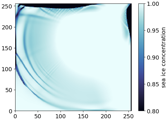
Figure 1 Simulated sea ice concentration generated by Veris after 1440 time steps of 10 min (equivalent to 10 d), driven by circular ocean surface currents and wind fields. The initial conditions included a uniform sea ice concentration of 1 and a sea ice thickness of 0.3 m. A reference simulation with the MITgcm, employing the same forcing, produced the same features (Fig. A2).

3.2 Benchmark Results

To evaluate the performance of Veris, a series of idealized and scalable benchmark experiments were conducted. These experiments were performed on a rectangular grid with varying process count and problem size, utilizing the scaled forcing fields described in Sect. 3.1. The benchmarks serve two primary purposes. First, they compare the performance of Veris to the Fortran reference, assessing the impact of transitioning from Fortran to Python. Second, the benchmarks analyze the scaling behavior of Veris with increasing process count and domain size. Additionally, Veris running on a GPU is compared to the Fortran reference across various parallel CPU configurations, focusing on both time to solution and total power consumption.

The benchmarks are performed over 20 time steps. During the first time step, the compilation process with JAX's JIT compiler introduces significant overhead. To properly evaluate the model performance, the first time step is therefore discarded. The absolute compilation time for CPU-based processes ranges from 2.0 to 32.2 s and the relative compilation time ranges from 1.0 to 10.4 model iterations. For GPU-based processes, absolute and relative compilation times range from 2.1 to 32.4 s and from 2.1 to 6.2 model iterations, respectively.

For both Veris and the MITgcm, the full model is run with thermodynamics disabled at runtime (i.e., it is compiled but not run), and the reported timings exclude thermodynamics, initialization, and finalization. This approach is justified because thermodynamic calculations are computationally less expensive and negligible compared to the dynamics. The models are compared using the aEVP solver with 120 subcycling iterations.

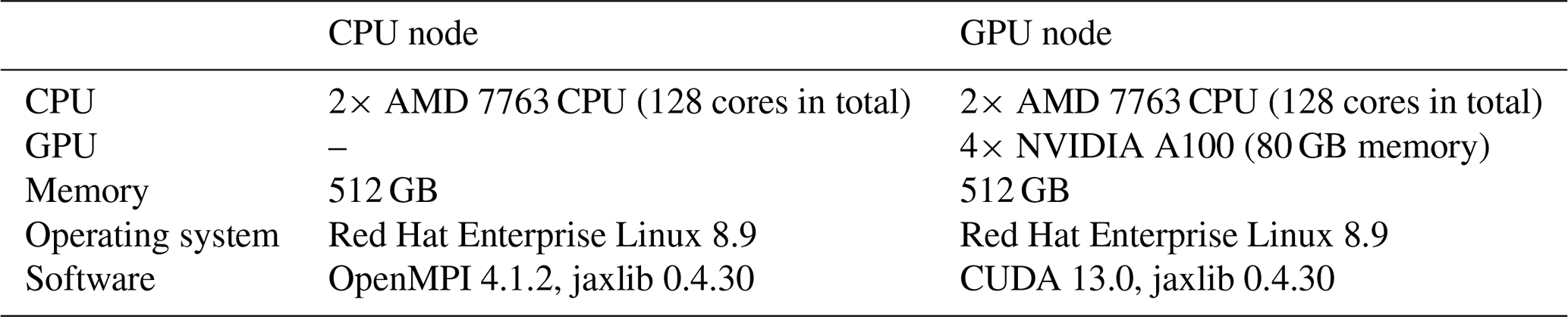
The benchmarks are run on two different nodes of the HPC Levante, a supercomputer of the German Climate Computing Center (DKRZ). The specifications of the different node types are listed in Table 1.

Table 1 Specifications of the benchmark platforms. A GPU node contains both GPUs and CPUs. Even in GPU-based processes, CPU cores are necessary, for example for transferring data from disk to GPU memory, where computations are performed.

3.2.1 Scaling With Number of Processes

This section analyzes the performance scaling with respect to the number of processes (Fig. 2). The number of processes corresponds to the number of partitioning regions and is specified by the scheduler of the HPC system used for benchmarking. A CPU-based process is bound to a single CPU-core, while a GPU-based process is bound to a single GPU, with JAX kernels automatically exploiting all available threads in the GPU. For the CPU-based simulations, grids with approximately 10⁶ and 9.4×10⁶ grid cells were evaluated, hereafter referred to as the 1 M and 9.4 M grids. The 1 M grid experiments were conducted on a single node. Both Veris and the MITgcm exhibit a similar initial increase in performance with rising core counts, a plateau in performance between 8–64 and 16–64 processes, respectively, and a renewed increase at 128 processes. For Veris, increasing the process count requires additional memory due to JAX's compilation cache, larger communication buffers, and the overhead associated with Python objects and metadata. For the 9.4 M grid, this necessitates distributing the simulation across multiple nodes, with at most 16 processes per node. The MITgcm is able to run the 9.4 M grid on a single node; however, this configuration results in a substantial performance degradation and poorer scaling behavior (not shown). When the simulation is distributed across multiple nodes, the MITgcm outperforms Veris, achieving approximately a fourfold speedup over Veris at 128 processes (Fig. 2). When constrained to a single node, the MITgcm exhibits both worse scaling and lower absolute performance than Veris running across multiple nodes.

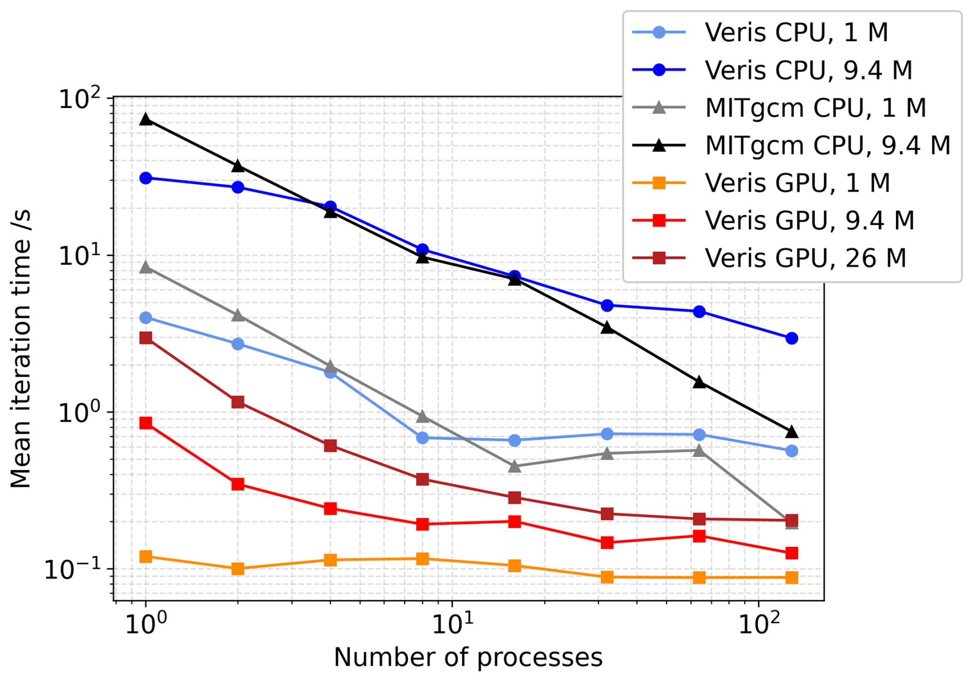
Figure 2 Scaling of mean iteration time with process count for Veris and the MITgcm sea ice component for varying problem sizes (1 M =10⁶ grid cells), calculated over 20 iterations steps.

The GPU-based simulations substantially outperform the CPU-based simulations, with a single GPU process matching the performance of the MITgcm running on hundreds of CPU cores. Increasing the number of processes introduces additional communication overhead, which is more pronounced for GPUs than for CPUs because GPUs do not share memory and therefore require explicit data movement between devices for communication. As a result, performance scaling on GPUs is strongly dependent on problem size. For the 1 M grid, increasing the GPU count from 1 to 128 yields only marginal performance gains. The 9.4 M grid exhibits improved scaling but still approaches saturation. In this context, saturation refers to the limited increase in performance with process count, which is attributed to the large communication overhead exceeding computational efficiency. Among the tested configurations, the 26 M grid, which contains approximately 26×10⁶ grid cells, shows the best scaling behavior, with a consistent performance increase as the GPU count increases. However, even for this grid, only limited performance gains are observed for higher GPU counts, indicating saturation. Overall, these results demonstrate the substantial performance benefits of GPU-based execution compared to CPU-based systems. They further suggest that GPU parallelization becomes increasingly effective for larger problem sizes, highlighting the potential of Veris for very large-scale simulations on GPU-accelerated architectures.

3.2.2 Scaling With Domain Size

In addition to the scaling with respect to process count, we performed benchmarks to analyze the dependence of performance on domain size for single-process simulations (Fig. 3). Veris exhibits scaling behavior consistent with that of the Fortran reference implementation. Scaling in this section refers to the increase in time to solution with domain size. When using Numpy as the backend, Veris is approximately five times slower than the MITgcm for domain sizes 10⁶ or smaller and around 15 times slower on domain sizes 10⁷ or larger. With the JAX backend, Veris consistently outperforms the Fortran reference, with mean iteration times approximately a factor of two smaller for grids larger than 10⁶ cells.

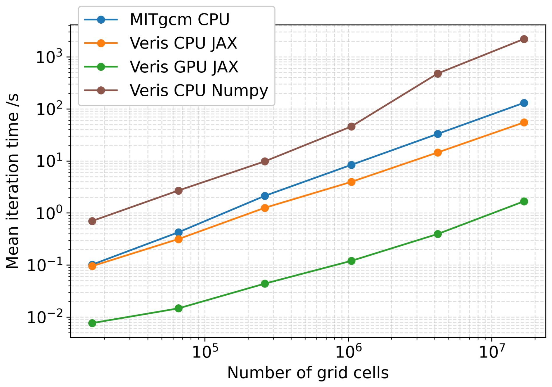
Figure 3 Benchmark results comparing the scaling of mean iteration time with grid size for Veris and the MITgcm, calculated over 20 iteration steps.

Simulations executed on a single GPU demonstrate both a substantial absolute performance increase and good scaling with increasing grid size. These results highlight the effectiveness of GPU-based execution for large domains and further emphasize the suitability of the JAX-based implementation for large-scale, high-resolution sea ice simulations.

3.2.3 Power Consumption

In addition to time to solution, energy consumption is a key metric in high-performance computing. Reducing energy usage not only lowers operational costs but also mitigates the carbon footprint of large-scale simulations. One promising approach for improving energy efficiency is to replace large numbers of CPU cores with a smaller number of GPUs, which can provide substantially higher performance per watt.

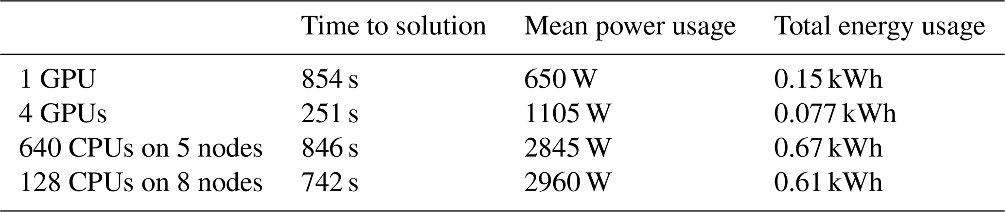
For the power consumption benchmark, we selected the 9.4 M grid configuration and measured the energy usage over 1000 iterations. The reference simulation was performed using a single GPU. For the MITgcm, CPU-based simulations were conducted that matched the time to solution of the single-GPU configuration, using both the minimum number of nodes and the minimum number of CPU cores (Table 2). In addition, a simulation utilizing all 4 GPUs available on a single GPU node was performed. The time to solution of the single-GPU run was matched by a configuration using 640 CPU cores across 5 nodes and by a configuration using 128 CPU cores across 8 nodes. Both CPU-based simulations exhibited similar total energy consumption, requiring approximately 4–4.5 times the energy of the single-GPU simulation. When all four GPUs on a GPU node were utilized, the total energy consumption was reduced by a factor of two relative to the single-GPU simulation. These results demonstrate the substantial energy-efficiency advantages of GPU-based execution for large-scale sea ice simulations.

Table 2 Power consumption for Veris running on 1 and 4 GPUs (on the same GPU node) and the MITgcm sea ice component running in various CPU-based configurations. CPU here refers to a single CPU-core process. This simulation is using 9.4×10⁶ grid cells and 1000 iterations. The power usage is reported by Levante's built-in power tracking system.

4 Discussion

The performance benchmarks of both the MITgcm and Veris showed a strong dependence of model performance on the underlying HPC configuration. Identical numbers of CPU-cores can yield substantially different solution times, depending on how processes are distributed across the nodes and mapped to cores within a node. This shows that optimal performance requires not only efficient model implementations, but also careful tuning of the parallel configuration to the HPC system. Such tuning involves the choice of processor grids, node layouts, and process placement strategies, and presupposes a detailed understanding of the HPC system. The strong dependence of model performance on HPC configuration indicates that the model is highly bandwidth-bound, a limitation that has also been identified as a major bottleneck in previous studies of Fortran implementations of the EVP solver (Rasmussen et al., 2024).

For established Fortran-based models, MPI-based communication has been extensively optimized over years of development and use. However, it is still identified as another major bottleneck of performance (Rasmussen et al., 2024). In contrast, distributed execution in JAX is an active area of development, and there is considerable potential for further improvements in communication backends and process orchestration. The results of this study therefore highlight both the promise of JAX for climate modeling in HPC environments and the importance of systematic communication analysis and optimization. The strong impact of communication overhead is also reflected in the early saturation observed in GPU-based simulations for smaller problem sizes. Given that Veris consistently outperforms the MITgcm at small process counts, even in CPU-based benchmarks, further advances in JAX communication could enable Veris to outperform its Fortran reference in strongly parallel regimes as well.

The benchmarks further reveal a significant performance benefit when transitioning from CPU-only systems to GPU-accelerated architectures, underscoring the growing importance of GPUs for climate modeling. This is particularly advantageous in the context of JAX, which is accelerator-agnostic and allows newly developed model components to run on GPUs without additional code modifications.

The GPU-based simulations exhibit the expected scaling behavior, with improved efficiency for larger domains, consistent with the high communication overhead associated with multi-GPU execution. This emphasizes the suitability of multi-GPU configurations for high-resolution modeling. Moreover, the power consumption measurements demonstrate that GPU-based Veris simulations can achieve comparable or superior performance at a fraction of the energy cost of CPU-based MITgcm runs, showing the potential of GPU-accelerated Python models to reduce both the operational cost and the carbon footprint of climate simulations.

The sensitivity of model performance to the chosen HPC configuration is less pronounced for GPU-based simulations than for CPU-based simulations. This is partly attributable to the fact that JAX is currently better optimized for GPU execution than for distributed CPU-based simulations. These results suggest that JAX holds further promise for CPU-based climate modeling, given the ongoing development of JAX and its distributed runtime, which may lead to further performance improvements in the future.

The choice of hardware, including the specific GPU and CPU, affects both model performance and energy consumption (Rasmussen et al., 2024). In addition to performance, cost is an important factor when evaluating the usefulness of GPU- and CPU-based architectures. Here, we used hardware available at the DKRZ, a representative and widely used HPC system for climate research in Germany. The NVIDIA A100 80 GB GPU installed at the DKRZ typically costs USD 20 000–30 000, while the AMD 7763 CPU retails for approximately USD 3000–4000.

The initial version of Veris was configured for integration with Veros to form a coupled sea ice-ocean model. This version and its coupling to Veros are described in detail in Gärtner (2023). To enable parallel execution with JAX, however, Veris was restructured around JAX's sharded arrays and is no longer compatible with Veros in this updated version. The coupled Veros-Veris model can be executed using NumPy on both single and multiple processes, and with JAX on a single process. Future work on enabling parallel execution of the coupled model with JAX will require either the development of a Veros-compatible communication mechanism within compiled loops (see Sect. 2.4) or a redesign of Veros' communication infrastructure around JAX's sharded arrays.

5 Summary and Conclusion

By translating the sea ice component of the MITgcm into Python, we developed Veris, a fully Python-based sea ice model. Veris can be coupled to the Python-based ocean model Veros, forming a coupled ocean–sea ice model implemented entirely in Python. This version supports parallel execution with Numpy and single-process execution with JAX on both CPU and GPU architectures. Although this version does not support distributed parallelism for JAX-based simulations, the benchmarks already demonstrated the potential JAX has for large-scale simulations, given the substantial performance gains of GPU execution.

To enable scalable parallelism, the Veris infrastructure was subsequently redesigned around JAX's sharded array framework, allowing distributed execution on both CPU- and GPU-based systems. The benchmarks presented in this study demonstrate the great potential of JAX for climate modeling. At small process counts, Veris outperforms the MITgcm. At larger process counts, communication overhead becomes the dominant performance factor, and the MITgcm runs faster than Veris. This sensitivity on the communication framework was also evident in the dependence of performance on specific HPC configurations. Whereas MPI-based communication in the MITgcm benefits from long-standing optimizations, communication in JAX-based distributed systems is still evolving. The superior performance of Veris at low process counts indicates strong potential for large-scale applications, particularly as JAX's distributed runtime continues to be developed and optimized.

GPU execution yields particularly strong performance benfits. A single-GPU run of Veris matches the performance of the MITgcm running on hundreds of CPU cores across multiple nodes, while consuming substantially less energy. These results demonstrate not only the competitiveness of Python-based, JAX-accelerated models in terms of time to solution, but also their potential to significantly improve the energy efficiency of climate simulations.

In summary, Veris demonstrates that Python, when combined with JAX, can support high-performance, scalable, and energy-efficient sea ice modeling. These findings suggest that JAX-based climate models are a promising pathway towards modern HPC workflows, with the prospect of further performance gains as communication backends and distributed execution frameworks continue to improve.

Appendix A: Code Verification, Comparison of Simulated Sea Ice between Veris and the MITgcm

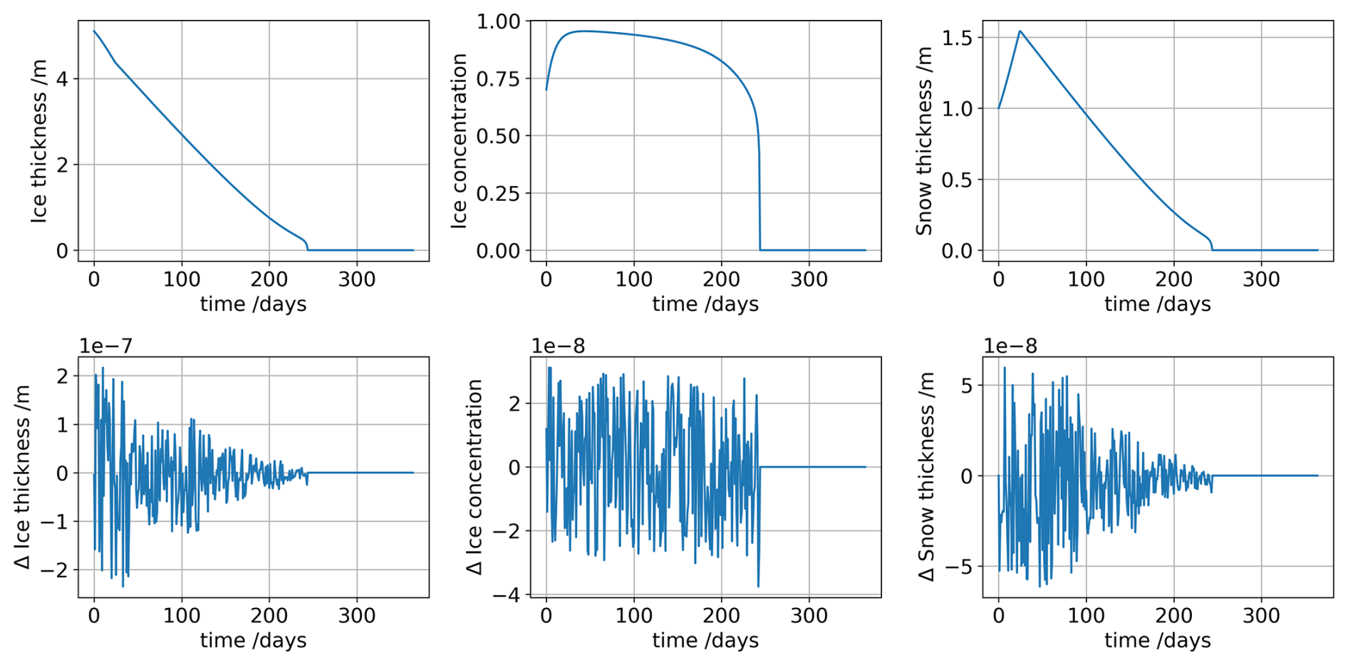
Figure A1 Example benchmark simulation used for verifying the thermodynamic component of Veris. Top row: Thermodynamic evolution of ice thickness, ice concentration, and snow thickness simulated by Veris. Bottom row: Comparison of the simulated sea ice between Veris and the MITgcm employing the same initial and forcing conditions. This figure is representative of the results of different thermodynamic benchmark comparisons using different initial and forcing conditions.

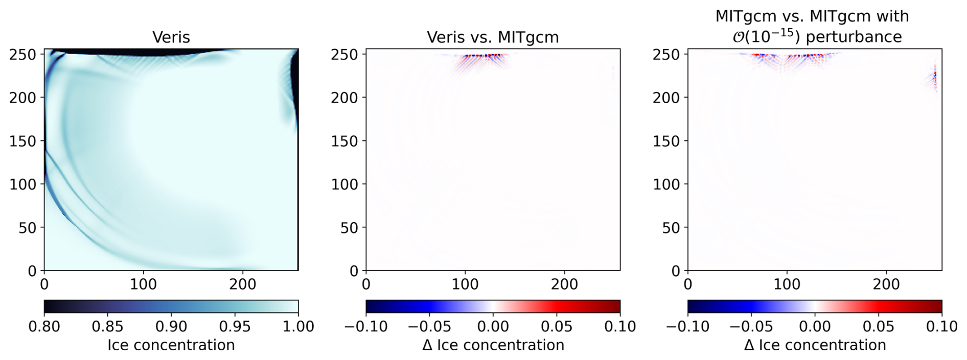
Figure A2 Example benchmark simulation used for verifying the dynamic component of Veris. Left panel: Sea ice concentration simulated by Veris after 1000 10 min time steps using forcing fields designed to induce ice fracturing. Middle panel: Comparison of the simulated sea ice between Veris and the MITgcm employing the same initial and forcing conditions. Right panel: As a reference for acceptable divergence, the difference between the MITgcm and a rerun of the MITgcm with perturbed initial and forcing conditions is shown. This figure is representative of the results of different dynamic benchmark comparisons using different grid sizes and initial and forcing conditions.