HydroBlocks-MSSUBv0.1: a multiscale approach for simulating lateral subsurface flow dynamics in Land Surface Models

Groundwater is critical in the hydrological cycle, impacting water supply, agriculture, and climate regulation. However, current Land Surface Models (LSMs) often struggle to accurately represent the multiple spatial scales of subsurface flow primarily due to the complexity of incorporating sufficient and yet efficiently surface heterogeneity, which significantly influences subsurface dynamics. Accurately modeling this heterogeneity requires substantial computational resources, often making it challenging to achieve in practice. This study introduces a multiscale approach to address this limitation. The approach leverages the hierarchical clustering scheme of the HydroBlocks model to define hydrologically similar areas that the model uses to capture local, intermediate, and regional flow dynamics within regional units, which interact laterally based on hydraulic gradients and soil properties. The proposed method is compared against a benchmark simulation with 1.4 million modeling units – 34 times the number of tiles in the multiscale experiment. The results show consistency in spatial distribution and a Pearson coefficient of correlation above 0.80 for the temporal variability of hydrological variables such as latent and sensible heat flux, surface runoff, and effective saturation at the root zone, demonstrating its ability to represent subsurface flow patterns adequately. The scheme, however, struggles to adequately represent volumetric water content at the bottom of the soil column, as evidenced by lower correlation coefficients, where the misrepresentation of elevation heterogeneity may play a larger role. This multiscale approach offers a computationally efficient way to incorporate detailed subsurface processes into large-scale hydrological simulations, improving our understanding of water cycle dynamics and supporting informed water resource management.

1 Introduction

Groundwater is critical in the hydrological cycle, impacting water supply, agriculture, ecosystems, climate regulation, drought resilience, and overall sustainability (Gorelick and Zheng, 2015; Taylor et al., 2013). Its significance in Earth System Models (ESMs) relates to the dynamic interaction between the subsurface and the ocean, atmosphere, and the land surface. Subsurface flow influences surface water exchange, aquifer storage, and soil moisture redistribution, which significantly impact water and energy exchanges with the atmosphere and water balance in the vadose zone (Chen and Hu, 2004; Fan, 2015; Felfelani et al., 2021; de Graaf et al., 2015; Maxwell and Condon, 2016; Zeng et al., 2018).

Tóth's (1963) hierarchical classification categorizes subsurface flow into three primary flow systems: local, intermediate, and regional. Local flow refers to the shallow water movement within the same basin and hillslopes. In contrast, regional flow occurs at greater depths, extending beyond superficial watershed boundaries and connecting large-scale recharge to discharge zones. Intermediate flow occurs along the continuum between the latter two flows. This classification highlights how subsurface flow exhibits significant variations across spatial and temporal scales, influenced by landforms and subsurface properties. These variations lead to diverse water table dynamics and surface water and energy fluxes (Fan, 2015; Freeze and Witherspoon, 1967; de Graaf et al., 2015). Studies indicate that lateral flow can substantially impact water table depths, especially in regions with heterogeneous soil properties or varying topography, as seen in North Africa, the Arabian Peninsula, and other areas experiencing water table decline (Maxwell et al., 2015; Rihani et al., 2010; Zeng et al., 2018). Lateral flow also affects the spatial distribution of soil moisture along hillslopes, influencing surface water and groundwater interactions and, ultimately, maintaining the balance of groundwater systems. To accurately represent the hydrological cycle in Land Surface Models (LSMs), a comprehensive multiscale approach is essential to capture local to regional patterns of lateral subsurface flow.

The representation of subsurface dynamics in LSMs has advanced significantly in the last few decades due to the growth of high-performance computing and data availability. Multiple schemes to represent the two-way interaction between surface water and the subsurface in LSMs have been developed and implemented (Bisht et al., 2018; Blyth et al., 2021; Fan et al., 2007; Fan and Miguez-Macho, 2011; Fisher and Koven, 2020; Hoch et al., 2023; Maxwell et al., 2015; Miguez-Macho et al., 2007; Miguez-Macho and Fan, 2012a, b; Naz et al., 2023; Zampieri et al., 2012). These approaches vary from bucket and two-layered models to coupled groundwater frameworks and data-driven approaches. The first two types of approaches provide a simplified and computationally efficient representation of the subsurface system; the last two are more costly in data and computation but can offer the highest level of detail by solving the complete three-dimensional equations to capture subsurface dynamics better (Guay et al., 2013; Jing et al., 2018; Maxwell et al., 2014; Sulis et al., 2010).

Within a single basin, topography plays a critical role in subsurface fluxes. Elevation differences between valleys and ridges create hydraulic gradients, the primary drivers of subsurface flow (Cardenas and Jiang, 2010; Harvey and Bencala, 1993; Tóth, 1963). However, accurately capturing these dynamics in LSMs presents a challenge. Current LSM grids typically operate at coarse scales (tens to hundreds of kilometers), which are incompatible with the fine-scale variations in topography that govern local flow paths. Most LSMs also focus only on vertical flow processes within the soil column, and lateral flow is often neglected or simplified (Condon et al., 2021; Ji et al., 2017; Lam et al., 2011; Mendoza et al., 2015; Naz et al., 2023; Shrestha et al., 2015).

The modeling community has widely recognized the challenges of incorporating high-resolution to represent small-scale subsurface processes within large-scale simulations (Choi, 2013; Fisher and Koven, 2020; Zhang and Montgomery, 1994; Zhao and Li, 2015). In alignment with the findings of Barlage et al. (2021), finer spatial resolution enables better representation of topographic convergence zones and shallow water table dynamics. Their study demonstrates that resolving these features at convection-permitting scales leads to increased root-zone soil moisture, enhanced evapotranspiration, and improved feedbacks to the atmosphere, including reductions in temperature and precipitation biases. Several modern LSMs can numerically simulate subsurface flow dynamics with high spatial resolution. These models can explicitly represent variations in topography, soil properties, and vegetation cover, leading to more accurate simulations of water movement within a basin (Kollet and Maxwell, 2008; Maxwell et al., 2015). However, these high-resolution simulations are often computationally expensive and impractical for large-scale applications like ESMs. The complexity of solving three-dimensional flow equations across large extents with high spatial resolution pushes computational resources to their limits.

One promising strategy for accounting for small-scale processes in large-scale simulations involves implementing tiling schemes. These schemes essentially group together hydrologically similar areas based on common characteristics such as soil type, land cover, topography, etc., that will respond similarly under equivalent meteorological forcing within an LSM grid cell, reducing the overall number of modeling units and leading to improved computational efficiency (Chaney et al., 2016, 2018, 2021; Flügel, 1995; Manrique-Suñén et al., 2013; Melton et al., 2017; Pilotto et al., 2017). This allows the incorporation of small-scale heterogeneity within large-scale simulations without sacrificing computational feasibility. Tiling schemes can bridge the gap between computationally expensive high-resolution models and practical large-scale simulations (Blyth et al., 2021; Clark et al., 2015; Fisher and Koven, 2020). Furthermore, a potential advantage of tiling schemes is that they simulate lateral subsurface movement by allowing water exchange between neighboring tiles. This exchange can be based on factors like the hydraulic gradient or other relevant parameters specific to the hydrological setting. Moreover, tiling schemes offer scalability: the number and complexity of tiles within a grid cell can be adjusted based on the model's needs and available computational resources. This allows for efficient simulations at both coarse and fine scales.

This study addresses the need for tiling schemes to represent the lateral interaction of subsurface flow within LSMs at various spatial scales. Specifically, it incorporates intermediate and regional flow into an existing modeling framework, HydroBlocks, leveraging its hierarchical clustering scheme to define tiles that interact laterally to account for local lateral flow. These model tiles are then grouped into regional units that can interact laterally across different spatial scales. The properties governing water movement within the new regional units are determined by the combined characteristics of the tiles (i.e., soil hydraulic properties), weighted by their relative area coverage. The proposed methodology is compared against a benchmark of the base HydroBlocks model with a significantly larger number of tiles. This approach aims to represent a fully distributed solution that facilitates tile interaction between parallel processes and regional flows throughout the entire simulation domain. This comparison shows that the new multiscale scheme for lateral flow converges toward the synthetic truth after a long-term simulation. Furthermore, our multiscale scheme is relatively efficient in terms of computational requirements. A 150 year hourly simulation for a 1°×1° domain using high spatial resolution (∼30 m) data with 40 700 tiles and a constant soil column depth of 10 m divided into six variable-depth layers takes 12 % of the time that the benchmark simulation with 1.4 million tiles takes to run.

2 Data and Methods

2.1 Study area and input Datasets

Figure 1 shows the selected study domain located in Southwest Colorado in a 1°×1° box. The area, extending approximately 8750 km², contains the headwaters of the Gunnison River drainage area, characterized by a heterogeneous hydrological system influenced by elevation, precipitation, and land cover. The river network includes the Taylor River, East River, Tomichi Creek, and the Blue Mesa Reservoir. The elevation within the domain ranges between 2100 and 4400 m above sea level (m a.s.l.), with the main rivers draining west (Fig. 1b). Land cover classification indicates barren primarily and sparsely vegetated areas in the highlands, as shown in Fig. 1c. Lastly, clay content at the surface suggests low-permeability soils near the stream areas and higher permeability towards the ridges (Fig. 1d), benefiting surface drainage and nutrient retention. Precipitation patterns vary significantly across the domain, with a declining gradient from west to east, approximating 496 mm yr⁻¹ over the entire region (Fig. 1e).

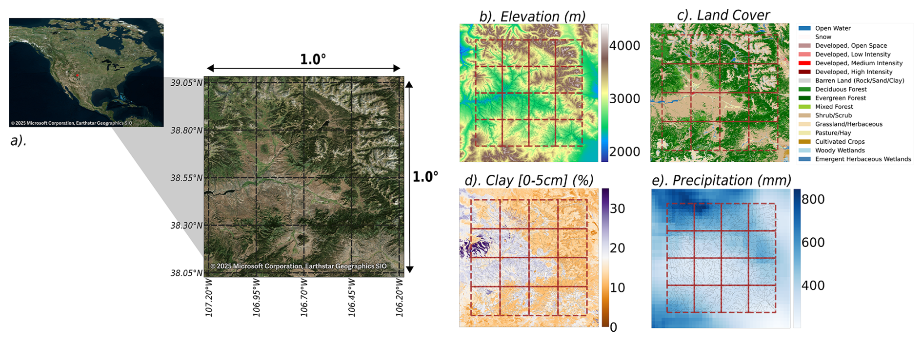
Figure 1 Study domain in Colorado, USA, in a 1°×1° box. (a) Satellite image of the study area divided by a 0.25° width grid showing the headwaters of the Gunnison River catchment (from Bing Maps, Microsoft. Retrieved 1 March 2025). (b) Elevation from the National Elevation Dataset (NED) and stream network. (c) Land cover classification from the National Land Cover Database (NLCD) with predominant barren areas. (d) Soil clay content (from 30 m resolution POLARIS dataset) shows higher percentages in the riparian zones and west-draining catchments. (e) Mean annual precipitation obtained from Princeton Climate Forcing (PCF) shows higher rates towards the north-west.

We used this study domain to test the representation of key hydrological processes at local, intermediate, and regional scales by allowing lateral subsurface water exchange between simulation units within the basin and between adjacent basins within the HydroBlocks framework. Furthermore, our proposed methodology can be scaled to conduct simulations at continental domains, following the same connectivity principles between parallel processes in High-Performance Computing (HPC) systems.

In this study, we used high spatial resolution and publicly available databases to parametrize Hydroblocks and explore the validity of the proposed multiscale methodology. The experiments were run over the study domain at an hourly time step over 150 years of simulation time. The data sets for topography, soil features, meteorology, and land cover used to drive HydroBlocks are described below.

Elevation: The National Elevation Dataset (NED; now known as 3DEP), maintained by the USGS, compiles comprehensive elevation data for the United States and surrounding areas. Data sources for this dataset include various USGS topographic surveys supplemented by lidar collections, high-resolution aerial photography, and other public and private sources (Gesch et al., 2018). The NED30 (∼30 m resolution) digital elevation model was sink-filled and used to define the river network and drainage areas for the simulation domain.

Soil Properties: To parametrize the soil column, we used POLARIS (Chaney et al., 2019), a database of ∼30 m probabilistic soil property maps over the contiguous United States, covering variables such as soil texture, organic matter, pH, saturated hydraulic conductivity, and water retention curve parameters up to 2 m deep, for deeper soil layers, we adopted a linear extrapolation. In POLARIS, each ∼30 m grid cell is assigned probabilities for various soil series, integrated with vertical soil profile data. This process calculates minimum, maximum, weighted average, and weighted variance for each cell, defining a beta distribution for soil parameters at different depths. The median values for porosity (θ_s), wilting point (θ_wp), field capacity (θ_fc), and saturated hydraulic conductivity (K_sat) are derived from these distributions. These values are then used to compute saturation suction (ψ_sat) and the inverse of the pore size distribution index (λ), which are inputs for the Campbell (1974) water retention model (Chaney et al., 2018). For the subsurface processes in this experiment, we considered a 10 m deep soil column everywhere, divided into six layers of variable depths: 0.05, 0.1, 0.35, 1.0, 1.5, and 7 m.

Although the chosen depth of the soil column is mostly arbitrary, we consider 10 m sufficient to evaluate the influence of lateral subsurface flows over land surface processes. 10 m is not a strict or universal cutoff, but we have adopted it as a reasonable approximation according to previous studies (Fan et al., 2013; Kollet and Maxwell, 2008; Shokri-Kuehni et al., 2020; Whittington and Price, 2006), where it has been shown that land-surface processes are considered not water-limited when the water table is near the surface, as capillary rise can supply water to the root zone, reducing water stress for plants. And conversely, surface processes are viewed as water-limited when the water table is deep, as they rely entirely on precipitation.

Meteorology: Atmospheric forcing data, including precipitation, air temperature, radiation, and wind speed, over the contiguous United States (CONUS) were obtained from the Princeton Climate Forcing (PCF) dataset at a $\mathrm{1}/\mathrm{32}$° spatial resolution (∼3 km) and at an hourly temporal scale from 2010 to 2019 (Pan et al., 2016).

Land Cover: Land cover data was obtained from the National Land Cover Database (NLCD) at ∼30 m resolution, a product based on a modified Anderson Level II classification system and 16 classes (Homer et al., 2015).

2.2 Land Surface Model: HydroBlocks v0.2

HydroBlocks v0.2 (Chaney et al., 2021) is a land surface modeling framework that addresses the challenges associated with accurately representing sub-grid heterogeneity in LSMs. The model effectively clusters spatial covariates for soil properties, topographic features, and meteorological variables to reduce the computational expense of resolving a high spatial-resolution LSM (Chaney et al., 2016). This is important, as a failure to represent sub-grid heterogeneity can lead to potential errors in simulated water fluxes and ecosystem dynamics, especially in areas with steep terrain or high spatial variability in soil properties (Clark et al., 2015; Fisher and Koven, 2020; Giorgi and Avissar, 1997; Torres-Rojas et al., 2022).

The Hierarchical Multivariate Clustering scheme (HMC) employed by HydroBlocks to derive tiles from available high-spatial resolution datasets is a key feature that significantly reduces the number of computational units while preserving essential local-scale processes in large-scale simulations.

Figure 2 shows the main steps of HydroBlocks' HMC algorithm. First, the domain is divided into macroscale polygons for parallel computing. Each subdivision comprises self-contained watersheds that are then grouped into k clusters of watersheds based on specific watershed-aggregated spatial covariates. Each cluster of watersheds is further discretized into height bands to differentiate between streams, valleys, and hilltops; for this step, every subsequent high band area is n times larger than the previous one, providing higher discretization near the streams. Finally, an average of p intra-band clusters is created for each high band based on soil parameters and land cover covariates representing field-scale heterogeneity (Chaney et al., 2021). It is important to acknowledge that the tiling structure, as pointed out in Torres-Rojas et al. (2022) and Chaney et al. (2016), obtained through the clustering mechanism – parameters k, p, and n – as well as the chosen proxies of spatial heterogeneity, will influence how close the model approximates the complexity and heterogeneity of the hydrological processes for the specific domain.

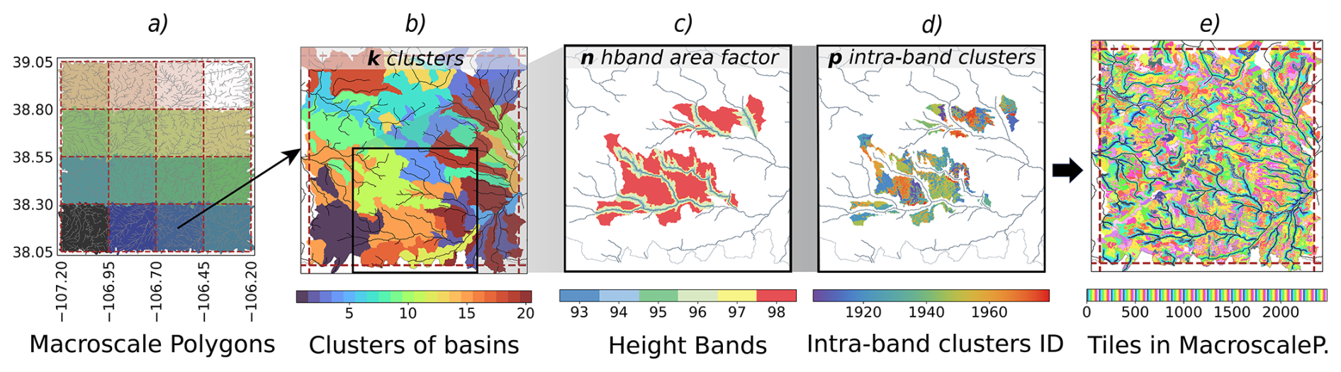
Figure 2 HydroBlocks HMC algorithm. (a) The domain is divided into 16 self-contained macroscale polygons; each color indicates a unique subdomain for parallel computing. (b) Macroscale polygon #3 is discretized into k=20 watershed clusters using large-scale heterogeneity proxies (latitude, longitude, drainage area). (c) cluster of watersheds #18 in the highlighted area in frame (b) is divided into height bands where the area of each subsequent band is n=2 times larger than the preceding one. (d) Each band is further discretized on average p=20 intra-band clusters across the height bands using proxies of field scale spatial heterogeneity (land cover, elevation, latitude, longitude, clay content); this frame shows the computed tiles for the uppermost height band. (e) The discretization is applied to each cluster of watersheds; consequently, each cluster contains a unique set of tiles. For this case, a total of 2480 tiles are defined for macroscale polygon #3.

2.3 Noah-MP

HydroBlocks uses the vertical 1D-column model Noah-MP (Niu et al., 2011), a comprehensive land surface resolving framework used to characterize hydrological and energy processes over land and the subsurface using a tile structure. The model includes physical representations of dynamic vegetation, canopy interception, multi-layer snowpack physics, and soil and hydrological processes. Combined with HydroBlocks, Noah-MP simulates various groundwater processes, including recharge, water table change, and baseflow for each of the tiles produced by the clustering algorithm (HMC). A simple groundwater model based on a TOPMODEL runoff scheme is also implemented to account for critical zone influence on runoff generation by linking soil moisture and water table dynamics (Niu et al., 2005, 2011). Water table depth depends on Noah-MP's parameterization, meaning that HydroBlocks does not override its position; rather, by modifying the soil moisture profile through lateral fluxes, we enable the model to adjust its dynamics. The adopted groundwater scheme (SIMTOP) assumes that soil moisture is in vertical hydrostatic equilibrium with a stationary water table, allowing the water table depth to be diagnosed directly from the soil moisture profile using the Clapp-Hornberger retention curve. This depth is then used to compute the fractional saturated area via an exponential function, reflecting how much of the landscape contributes to surface runoff (Niu et al., 2005). Both surface and subsurface runoff are generated as an exponential function of water table depth, with no explicit tracking of groundwater storage. This approach is computationally efficient and suitable for large-scale models, but because it relies on the equilibrium assumption, it captures only limited memory of antecedent weather events, focusing mainly on the current and recent hydrological conditions rather than long-term soil moisture storage.

At each time step, Noah-MP simulates soil moisture and vertical water flow in unsaturated soils across the soil layers using the one-dimensional Richards' equation (Eq. 1) to update the hydrological states of each tile.

$$\begin{array}{}\text{(1)}& {\displaystyle \frac{\partial \mathit{\theta }}{\partial t}}={\displaystyle \frac{\partial }{\partial z}}\left(D\left(\mathit{\theta }\right){\displaystyle \frac{\partial \mathit{\theta }}{\partial z}}\right)+{\displaystyle \frac{\partial K\left(\mathit{\theta }\right)}{\partial z}}-S,\end{array}$$

Where θ is the volumetric soil moisture content, D is the soil water diffusivity, K is the hydraulic conductivity, S represents sources and sinks of soil moisture, t is the time variable, and z indicates the vertical coordinate.

In Eq. (1), S accounts for soil surface infiltration, water loss due to plant transpiration, and surface evaporation. For the groundwater model, a no-drain condition at the bottom layer was set. However, water can be removed as lateral flux between soil columns as a new source/sink term G introduced in the HydroBlocks framework (Eq. 2).

$$\begin{array}{}\text{(2)}& {\displaystyle \frac{\partial {\mathit{\theta }}_i}{\partial t}}=-{\displaystyle \frac{\partial q_z}{\partial z_i}}-S_i-G_i,\end{array}$$

The new source/sink term G_i describes the computed lateral fluxes between adjacent tiles, assuming Darcy's law, which relates flow to the gradient of total hydraulic head under saturated conditions. This is represented as the divergence at the ith layer, as shown in Eq. (3).

$$\begin{array}{}\text{(3)}& G_i=-T_i{\displaystyle \frac{\mathrm{\Delta }{h}_i}{\mathrm{\Delta }x}}{\displaystyle \frac{w}{A_{\mathrm{T}}}}{\displaystyle \frac{\mathrm{1}}{\mathrm{\Delta }{z}_i}},\end{array}$$

Where T_i is the harmonic mean of the transmissivities between the interacting layers of two different tiles, Δh_i is the hydraulic head gradient at the ith layer, Δx is the horizontal distance between the centroids of the tile's areal polygons, w is the length of the shared perimeter between the tiles, A_T is the surface area of the corresponding polygon, and Δz is the thickness of the soil layer.

While the classic form of Darcy's law is strictly valid only under saturated conditions, where capillary forces are negligible, we extend its use to the unsaturated zone by incorporating a moisture-dependent hydraulic conductivity, as is done in the Richards' equation. In our implementation, assuming hydrostatic equilibrium in the vertical direction as a first-order approximation allows us to focus on the lateral hydraulic gradients while simplifying the vertical pressure distribution. This decomposition avoids the computational cost of solving the full 3D Richards' equation, while allowing for a continuous representation of lateral flow across both saturated and unsaturated layers.

2.4 A quasi-3D solution for subsurface flow in HydroBlocks

The model resolves soil moisture redistribution using a time-splitting scheme, separating the vertical and lateral components. Darcy's flux is used to solve the lateral flow after a fully implicit method, within Noah-MP, which resolves the vertical flow. The analysis is performed under the assumption that lateral flow in the unsaturated region can be represented using a Darcy flow with a moisture-dependent hydraulic conductivity; in unsaturated conditions, lateral flow is strongly limited due to the low hydraulic conductivity of the soil. Although this assumption is not required, it allows us to include representation of discontinuities in the saturated region of the soil column.

The decomposition of vertical and horizontal water flow follows a common approach used in large-scale land surface and hydrological models (Choi et al., 2007; Ji et al., 2017; Kuznetsov et al., 2012; Mao et al., 2019; Xie et al., 2020). The key assumption is that vertical dynamics can be separated from horizontal flow due to vertical flows being significantly larger than horizontal flows in the unsaturated region, and almost negligible in saturated conditions, where horizontal flow dominates. This operator-splitting strategy can introduce mass balance errors, but could be adequate under conditions where vertical flow dominates, and lateral gradients remain smooth (Gąsiorowski and Kolerski, 2020).

HydroBlocks does not explicitly define a hard separation between saturated and unsaturated layers. Instead, it relies on the 1D vertical solution of Richards' equation to simulate vertical water movement, and the simulated water content in each layer determines the pressure head and the hydraulic conductivity to be used in the computation of lateral flows. We apply this scheme regardless of the saturation conditions, but crucially, we use a soil moisture-dependent parameterization to ensure that in dry soils, lateral hydraulic conductivity and lateral flow are minimal, while maintaining a continuous representation of subsurface redistribution without explicitly segmenting saturated/unsaturated layers. While we acknowledge that some studies restrict lateral flow to saturated layers only, our framework can readily accommodate such a separation if needed. However, that level of constraint is not the focus of the present approach and should be explored further in future analysis.

2.5 Lateral subsurface flow: Multiscale Scheme (HydroBlocks-MSSUBv0.1)

The divergence term described in Sect. 2.3 accounts for lateral flow at a local scale, given that the tiles interact laterally within the same cluster of watersheds. However, a term that accounts for intermediate and regional flow paths has yet to be included. Here, we have developed a scheme to compute lateral flow for these longer flow paths following the same mechanism currently implemented in HydroBlocks to compute local lateral flow. To achieve this, we used the clusters of watersheds as Regional and Intermediate Subsurface Flow Units (RISFU) and a soil column underneath that interacts laterally with the neighboring areas at every layer, following Darcy's law to update the hydraulic state variables of the tiles within.

Figure 3 illustrates the proposed multiscale scheme for simulating lateral subsurface flow using HydroBlocks. The methodology involves five main stages: (1) Domain discretization into macroscale polygons and corresponding local tiles (using HydroBlocks' HMC), (2) Defining Intermediate and Regional Units (RISFU) to represent the subsurface system, (3) computing aggregated soil hydraulic properties to parametrize the RISFUs, (4) Computing subsurface lateral flow at different levels (regional, intermediate, and local), and (5) Updating vertical flow of the soil column within Noah-MP. Stages 1 and 2 are performed before the start of the simulation time, and Stages 3 to 5 are repeated for each timestep until the final simulation time step is reached. Details on each stage are presented below.

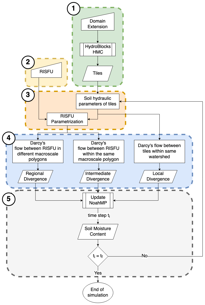
Figure 3 Proposed Multiscale Methodology flow chart. Step 1 consists of HydroBlocks' HMC to generate tiles per macroscale polygon. Step 2 is the generation of the RISFUs from the cluster of watersheds obtained through the HMC algorithm. Step 3 is the parametrization of the soil hydraulic properties of the RISFUs using the tiles inside them. Step 4 consists of computing the subsurface flow between the RISFUs within the same macroscale polygon (intermediate flow) and between RISFUs along the borders of different macroscale polygons (regional flow); local flow is the flow between tiles within the same cluster of watersheds, as is already implemented in HydroBlocks. Step 5 updates the divergence term in Richards' equation, resolved with Noah-MP, to include the three scales of subsurface flow for the next time step t_i until the end of the simulation t_f is reached.

2.5.1 Step 1. Domain discretization

As mentioned in Sect. 2.2, HydroBlocks' HMC initially divides the modeling domain into macroscale polygons to allow for efficient parallelization in High-Performance Computing systems. Each polygon represents a self-contained group of basins within a predefined bounding box. Subsequently, the HydroBlocks HMC algorithm generates a set of independent tiles, as described in Sect. 2.2 (see Fig. 2). These tiles serve as simulation units in the Noah-MP model, enabling the solution of water and energy fluxes.

2.5.2 Step 2. Definition of regional and intermediate subsurface flow units (RISFU)

Once each macroscale polygon has its own set of tiles, the next step involves discretizing the macroscale polygon on RISFUs (Fig. 4). For this experiment, these intermediate and regional units are chosen to be the same clusters of watersheds obtained from the intermediate step in the HMC algorithm. Consequently, each macroscale polygon is subdivided into a finite number of RISFUs representing the intermediate and regional-scale subsurface system's structure. The RISFUs do not need to be the same clusters of watersheds, and the extension, shape, and number can be modified to meet specific criteria, making this approach flexible for its implementation in large-scale simulations. For our case study, the number of clusters of watersheds generated and, consequently, the number of RISFUs is determined by the parameter k, chosen equal to 20. It is worth mentioning that the selection of parameter k and the proxies of large-scale heterogeneity will prescribe how the subsurface hydrological structure is represented in the LSM. In our study, the value of k was chosen empirically to capture the spatial heterogeneity of watershed-scale features while maintaining computational efficiency over a domain with significant elevation variability. In HydroBlocks, the clustering uses K-means applied to proxies for large-scale physical heterogeneity, including latitude, longitude, elevation, and flow accumulation area. Consequently, the parameter k accounts for the interaction of multiple spatial drivers rather than focusing solely on elevation variability alone.

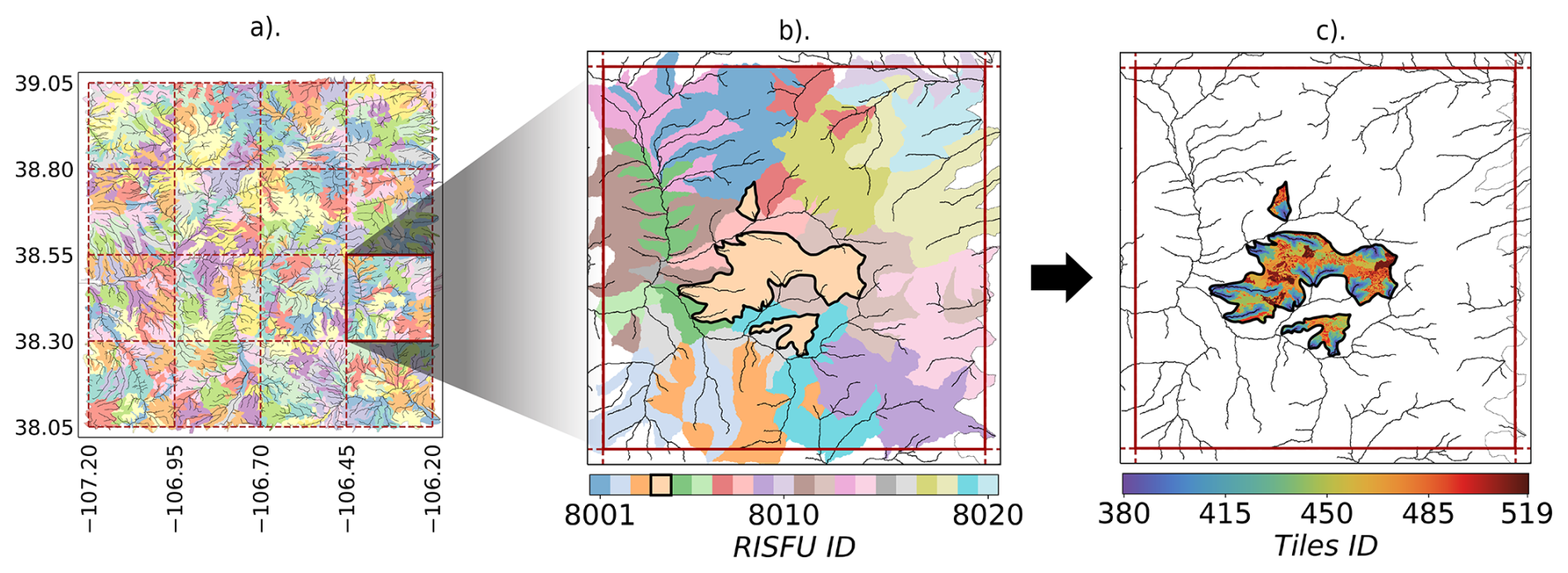
Figure 4 Regional and Intermediate Subsurface Flow Units (RISFUs). (a) Map of clusters of watersheds obtained from the HMC algorithm. For this experiment, the parameter k=20. (b) Each macroscale polygon contains a total of 20 RISFU, chosen to be the same as the clusters of watersheds in frame (a). The outlined area is a single RISFU. (c) The HydroBlocks tiles within the isolated RISFU from frame (b) that are used to compute the matrix of weights in Step 3a.

2.5.3 Step 3. Soil parameters Aggregation

The soil hydraulic properties of every layer of the RISFUs are determined by calculating the weighted average of the soil hydraulic properties from the corresponding layers of the individual tiles within each unit, as shown in Fig. 5 for saturated hydraulic conductivity (K_sat). The weights are set to be the fraction of the RISFU's area covered by each tile. This weight-averaging approach is applied to soil hydraulic parameters and state variables, including soil moisture, saturated water content, residual water content, and saturated hydraulic conductivity. By effectively combining the hydraulic properties of the constituent tiles, we create a representative characterization of the soil column for each RISFU. The procedure used to perform the aggregation of properties is detailed below.

Figure 5 Tile aggregation of soil hydraulic parameters to characterize RISFUs. (a) Saturated Hydraulic Conductivity (Ksat) map of tiles within a single RISFU. Values are for the root zone layer (0–5 cm). (b) Weighted-average Ksat for each RISFU (root zone layer). The process is repeated for all 20 RISFU in the macroscale polygon and for each layer of the soil column. (c) The process is then repeated across all 16 macroscale polygons to generate the map of the 1°×1° domain with the characterized RISFUs.

• (a)

  First, we compute the fraction of the area that each tile covers of the RISFU i. Each component a_ij represents the fraction of RISFU area A_R covered by the area A_T of tile j within that specific unit i to generate the matrix of area fractions [A] (Eq. 4).

  $$\begin{array}{}\text{(4)}& \left[A\right]=\left[\begin{array}{cccc}{a}_{\mathrm{11}}& a_{\mathrm{12}}& \mathrm{\cdots }& a_{\mathrm{1}j}\\ a_{\mathrm{21}}& a_{\mathrm{22}}& \mathrm{\cdots }& a_{\mathrm{2}j}\\ \mathrm{⋮}& \mathrm{⋮}& \mathrm{\ddots }& \mathrm{⋮}\\ a_{i\mathrm{1}}& a_{i\mathrm{2}}& \mathrm{\cdots }& a_{ij}\end{array}\right],a_{ij}={\displaystyle \frac{A_{{\mathrm{T}}_j}}{A_{{\mathrm{R}}_i}}},\end{array}$$
• (b)

  The RISFU's soil hydraulic properties (and state variables) P_R are computed as the weighted average of those of the tiles (P_T) within the RISFU boundaries. The process is repeated for each soil layer (Eq. 5).

  $$\begin{array}{}\text{(5)}& P_{\mathrm{R}}=\left[A\right]P_{\mathrm{T}},\end{array}$$
• (c)

  Every time step, the Soil Hydraulic Conductivity (K) of each RISFU layer is computed following the Brooks-Corey retention curve (Eq. 6).

  $$\begin{array}{}\text{(6)}& K\left(\mathit{\theta }\right)=K_{\text{sat}}{\left({\displaystyle \frac{\mathit{\psi }}{{\mathit{\psi }}_{\text{sat}}}}\right)}^{-\mathrm{2}-\mathrm{3}/b},\end{array}$$

  Where K_sat is the Saturated Hydraulic Conductivity, ψ is the matric potential, ψ_sat, b are model parameters, and θ is volumetric water content defined in Eq. (7) as:

  $$\begin{array}{}\text{(7)}& \mathit{\theta }=({\mathit{\theta }}_{\mathrm{s}}-{\mathit{\theta }}_{\mathrm{r}}){\left({\displaystyle \frac{\mathit{\psi }}{{\mathit{\psi }}_{\text{sat}}}}\right)}^{-\mathrm{1}/b}+{\mathit{\theta }}_{\mathrm{r}}\end{array}$$

  Where θ_s and θ_r are the saturated and residual water content, respectively.

2.5.4 Step 4. Subsurface Lateral Flow

For local subsurface flow (i.e., inter-tile level), HydroBlocks computes lateral flow between tiles connected within the same watershed using Darcy's law as introduced in Eq. (3). Figure 6 illustrates the process to estimate the hydraulic gradients between tiles (and between RISFUs). Every time step, the hydraulic head of each layer is estimated as the sum of the pore pressure and the elevation of the layer. The pore pressure is estimated following the relationship described in Clapp and Hornberger (1978). Similarly, hydraulic conductivity is represented as a function of updated conditions of water content in the layer, and it decays exponentially beyond 1.5 m.

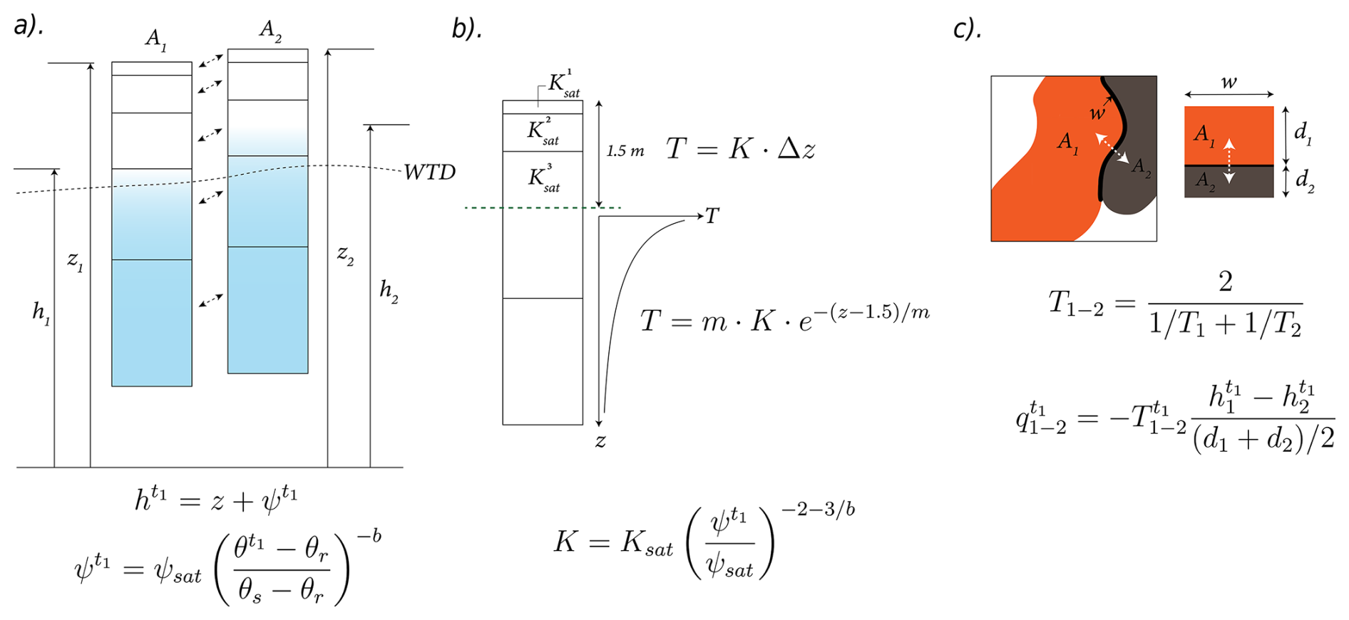
Figure 6 Lateral flow between two tiles in HydroBlocks. (a) Noah-MP computes the vertical redistribution of soil moisture for each soil column. Hydraulic head (h) is estimated as the sum of the elevation of the layer (z) and the matric potential (ψ) for soil moisture conditions for time step (t₁). (b) Lateral hydraulic conductivity (K) is updated every time step to account for the saturation conditions of the layers. Additionally, a decaying function to adjust K based on parameter (m) is applied to depths greater than 1.5 m. (c) Lateral flow between tiles 1 and 2 (q) is estimated based on the average transmissivity (T) and corresponding hydraulic head between the two layers of the soil columns and the distance between centroids $(d_{\mathrm{1}}+d_{\mathrm{2}})/\mathrm{2}$.

To calculate the distance in the direction of the flow, each tile is approximated to a rectangular shape of area A_T=dw, as shown in Fig. 7, where d is the side of the rectangle to be solved and w is the length of the shared perimeter between tiles, equal to the sum of the width of all grid cells in contact with the neighboring tile. This assumes that the flow in/out of the tile is homogeneous along the shared length and gets distributed across the entire area instantaneously, allowing us to define the horizontal traveling distance Δx for one of the tiles as half of the side d (Eq. 8).

$$\begin{array}{}\text{(8)}& \mathrm{\Delta }x={\displaystyle \frac{d_{\mathrm{1}}+d_{\mathrm{2}}}{\mathrm{2}}};d={\displaystyle \frac{A_{\mathrm{T}}}{w}},\end{array}$$

For regional and intermediate subsurface flow (i.e., RISFUs interaction), we use the same approach described for inter-tile interaction. We start by defining the horizontal distances between centroids of RISFUs. Similarly, these areas are also approximated to a rectangular shape, and horizontal distances and shared lengths are computed; this is done for the RISFU within the same macroscale polygon and for the RISFU at the perimeter in contact with adjacent macroscale polygons.

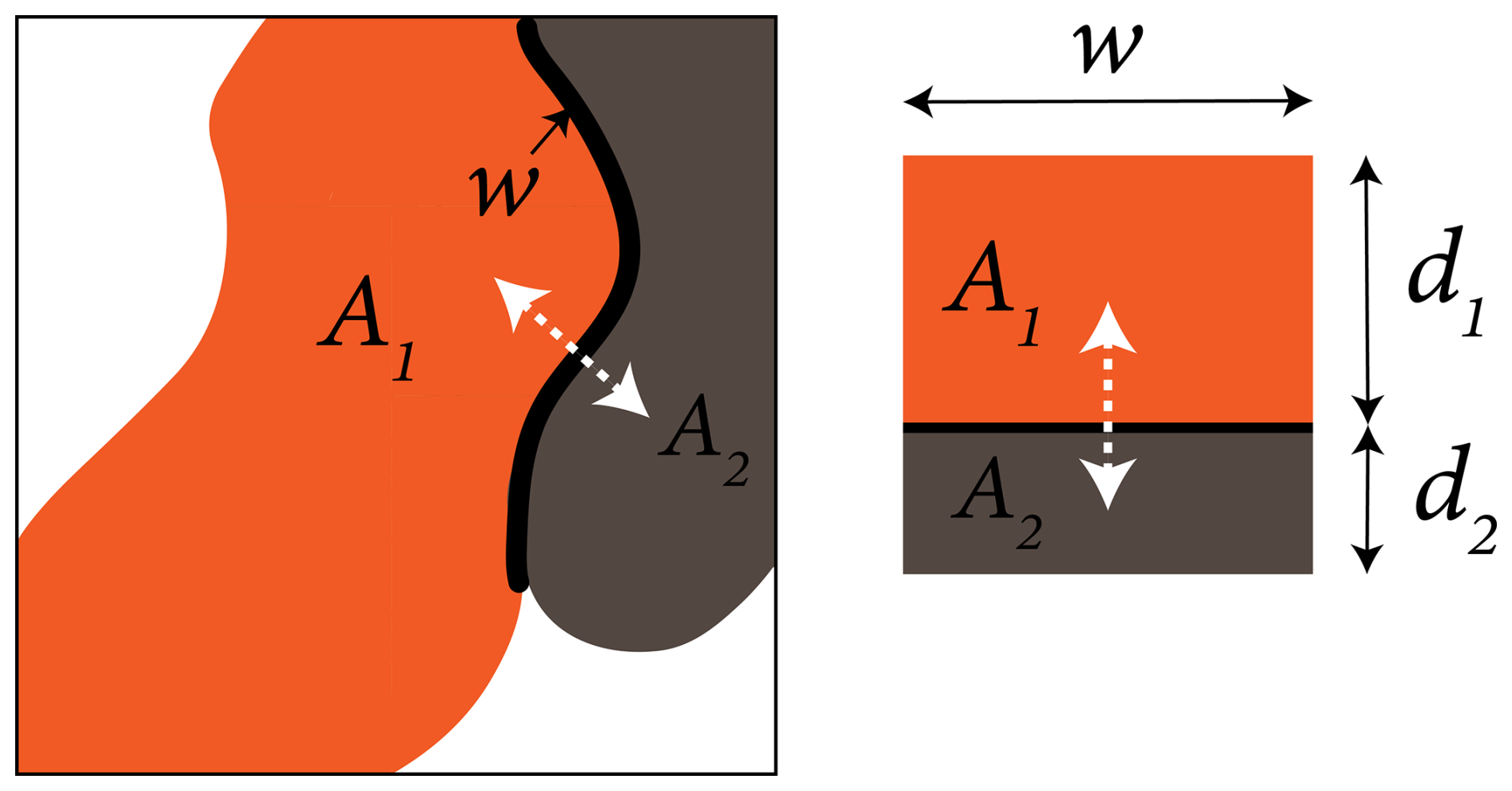
Figure 7 Area approximation for irregular tiles and RISFUs. Both tiles and RISFU are approximated to a rectangle of area A=dw. Where w is the shared perimeter length between two tiles or RISFUs. The horizontal traveling distance in the direction of the flow is then computed as $\mathrm{\Delta }x=d_{\mathrm{1}}/\mathrm{2}+d_{\mathrm{2}}/\mathrm{2}$.

The flux between tiles within the same basins (local scale) and between RISFU units (regional/intermediate scale) is computed for each time step, assuming Darcy's flow, as presented in Eq. (9). The net flow specifies the divergent subsurface flow for each tile or RISFU driven by the surrounding areas of the same scale.

$$\begin{array}{}\text{(9)}& Q_{\mathrm{R}}=\text{diag}\left(-\left[K_{\mathrm{R}}\right]{\displaystyle \frac{\left[\mathrm{\Delta }h\right]}{\left[\mathrm{\Delta }x\right]}}\right),\end{array}$$

Where Q_R is the net flow per RISFU, K_R is the harmonic mean of hydraulic conductivity between connected units, Δh and Δx are the hydraulic gradient and horizontal distance, respectively.

Hydraulic gradients (Δh): Lateral fluxes between RISFUs are computed using the hydraulic gradient, which is defined as the difference in total hydraulic head (h^t) between adjacent RISFUs, divided by the horizontal distance between their centroids (Δx). The hydraulic head (see Eq. 10) is defined as the sum of the pressure head (ψ^t) at the time step t and the elevation of the contributing layer (z). To define the pressure head (Eq. 11), we use the local soil moisture conditions (θ^t) at the specific layer in each RISFU and the representative residual and saturated soil moisture content, θ_r and θ_s respectively. Soil moisture conditions at each time step for each RISFU are averaged from the individual tiles, following the soil parameters aggregation described in Step 3.

$$\begin{array}{}\text{(10)}& {\displaystyle }{h}^t=z+{\mathit{\psi }}^t,\text{(11)}& {\displaystyle }{\mathit{\psi }}^t={\mathit{\psi }}_{\text{sat}}{\left({\displaystyle \frac{{\mathit{\theta }}^t-{\mathit{\theta }}_{\mathrm{r}}}{{\mathit{\theta }}_{\mathrm{s}}-{\mathit{\theta }}_{\mathrm{r}}}}\right)}^{-\mathrm{1}/b},\end{array}$$

Figure 8 illustrates the process of computing lateral flow at both intermediate and regional scales. Figure 8a presents a schematic example of four macroscale polygons with six interacting RISFUs. At a specific time step, the hydraulic gradient determines the subsurface flow (q) in the direction of the red arrows. The subscript denotes the interacting units, and the sign indicates the direction of the flow. For q2,1 and $-q\mathrm{2},\mathrm{1}$, the magnitude of the flow is equivalent, with the positive sign indicating flow from RISFU 2 to RISFU 1 in the former case. The net flow Q is then computed as the sum of all the flows (q) per unit. This is repeated for each layer of the soil column.

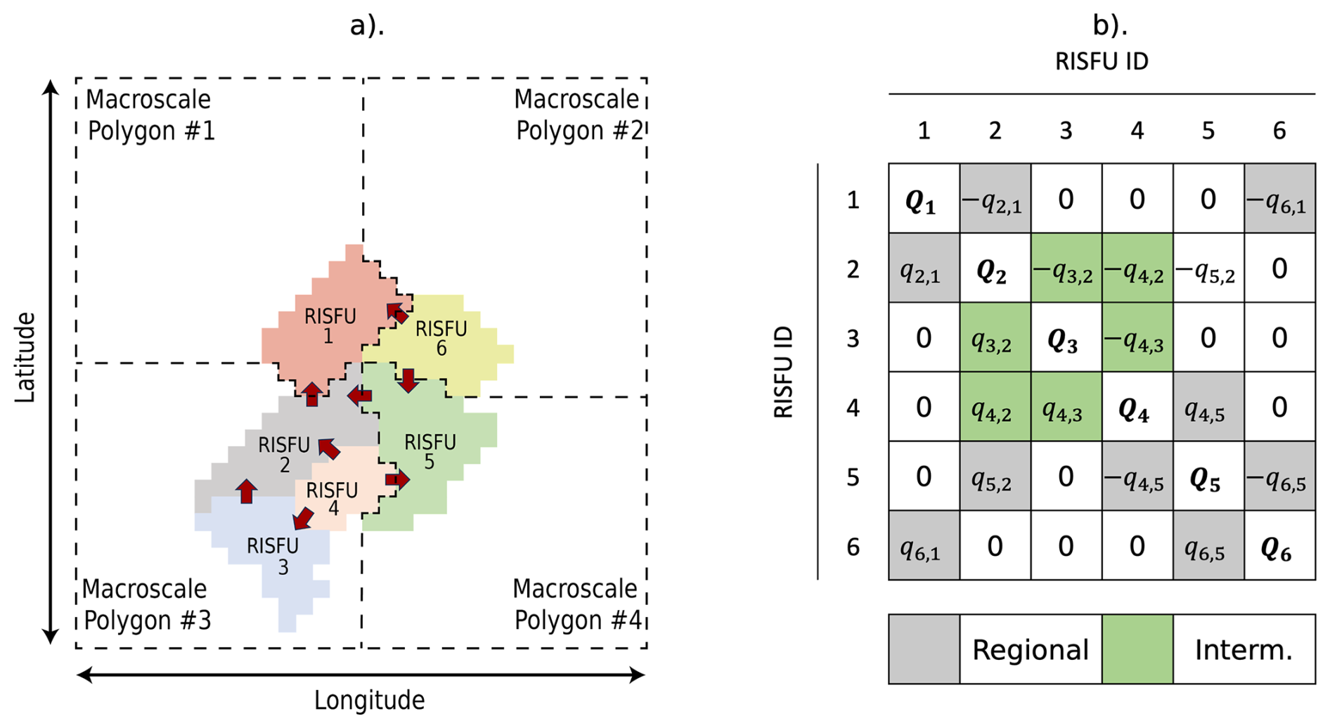
Figure 8 Lateral flow scheme for intermediate and regional scales. (a) An example of six RISFUs at four different macroscale polygons to visualize the process of computing net lateral flow between RISFUs. The direction of the flow at a specific time step is indicated by the red arrows. The perimeter of each macroscale polygon is represented by the dashed line. (b) Matrix of flows between interacting units. In grey are the flows between units at different macroscale polygons to represent regional scales, and in green are the intermediate flows. Units that are not laterally connected are assigned a zero flow. The net flow for each RISFU is then computed as the arithmetic sum of all the flows q in the same row.

Note that the boundaries of the macroscale polygons are purely schematic to illustrate an approximate division. However, the actual perimeter of the macroscale polygons follows that of self-contained watersheds, ensuring that no RISFU is divided between macroscale polygons.

The regional and intermediate net flows are redistributed among the tiles within each RISFU based on the matrix of areal fractions to obtain a single value for each tile, as shown in Eq. (12).

$$\begin{array}{}\text{(12)}& Q_{\mathrm{T}}=\left[A\right]Q_{\mathrm{R}},\end{array}$$

2.5.5 Step 5. Update Land Surface Model

The net flow per each tile T is then converted to a divergence G to be used as a source/sink term in the vertical solution of the differential equation in NOAH-MP following Eq. (13). The process is repeated each time step from stages 3 to 5 (see Fig. 3) using the solution for soil moisture content to update the hydraulic conductivity and hydraulic gradient until the simulation is completed.

$$\begin{array}{}\text{(13)}& G_{\mathrm{T}}=Q_{\mathrm{T}}{\displaystyle \frac{\mathrm{1}}{A_{\mathrm{T}}\mathrm{\Delta }z}},\end{array}$$

Where A_T is the surface area of each tile, and z is the layer's depth.

Following Eq. (2), where a new divergence term is added to include local lateral subsurface flow, the presented multiscale scheme updates the vertical solution of soil moisture with two extra divergence terms to represent intermediate and regional scales, shown in Eq. (14). The superscripts (R) (I) (L) indicate the Regional, Intermediate, and Local levels of each divergence term.

$$\begin{array}{}\text{(14)}& {\displaystyle \frac{\partial \mathit{\theta }}{\partial t}}=-{\displaystyle \frac{\partial q_z}{\partial z}}-G_{\mathrm{T}}^{\text{(R)}}-G_{\mathrm{T}}^{\text{(I)}}-G_{\mathrm{T}}^{\text{(L)}},\end{array}$$

2.6 Experimental Setup in HydroBlocks

To test our approach, we performed a set of experiments aimed at developing and validating an enhanced multiscale HydroBlocks framework designed to better capture water movement across different scales – ranging from local to regional. Our approach includes the extra two divergence terms described in Sect. 2.5 implemented within the tiling framework. We aim to evaluate the logical consistency of our scheme by selecting a 1°×1° domain, and applying HydroBlocks' HMC (see Sect. 2.2). The experiments were run at hourly time steps for a total of 150 years.

As illustrated in Fig. 9, the study area was partitioned into 16 macroscale polygons to facilitate parallelization. The domain is discretized into 40 700 tiles derived from high-resolution environmental data to capture the small-scale heterogeneity in elevation, land cover, and soil properties. The clusters of watersheds obtained through HydroBlocks' HMC for each macroscale polygon are then adopted as RISFU to represent the intermediate and regional units to model lateral subsurface flow.

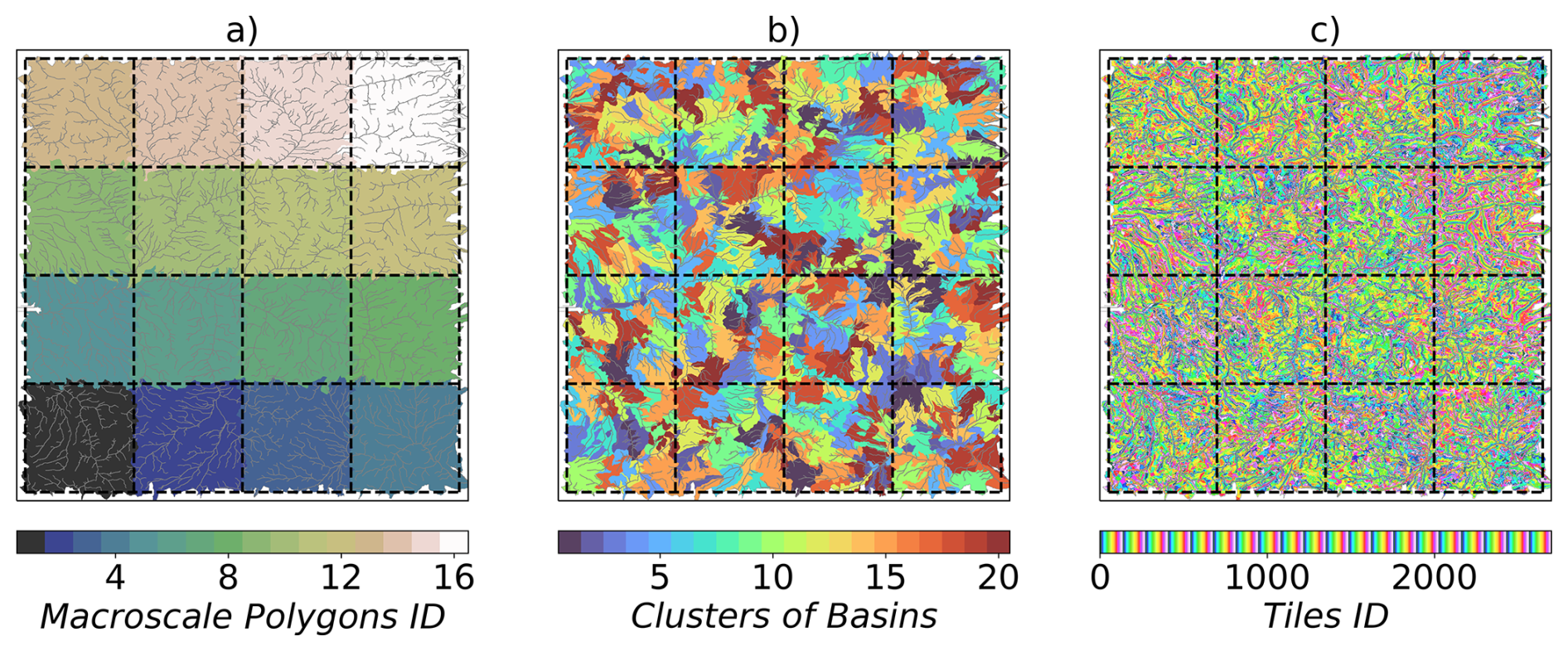
Figure 9 Experimental setup. (a) shows the domain divided into 16 self-contained macroscale polygons for parallel computing. (b) Map of the cluster of watersheds considering k=20 for the HMC algorithm in HydroBlocks. (c) Map of the tiles derived through the HMC algorithm in HydroBlocks; each macroscale polygon contains an average of 2500 tiles. HydroBlocks' HMC generates a total of 40 700 tiles using parameters k=20, n=2, p=20.

Figure 10 illustrates the simulated spatial mean for the variables of volumetric soil moisture content (SMC), sensible heat flux (SH), and water table elevation (ZWT) throughout the simulation period. For each iteration, we used ten years of hourly forcing data spanning from 1 January 2010 to 31 December 2019. The annual spatial mean for each experiment was compared to assess numerical stability, and the final year of simulation (2019) was employed to evaluate our multiscale scheme against the baseline and benchmark.

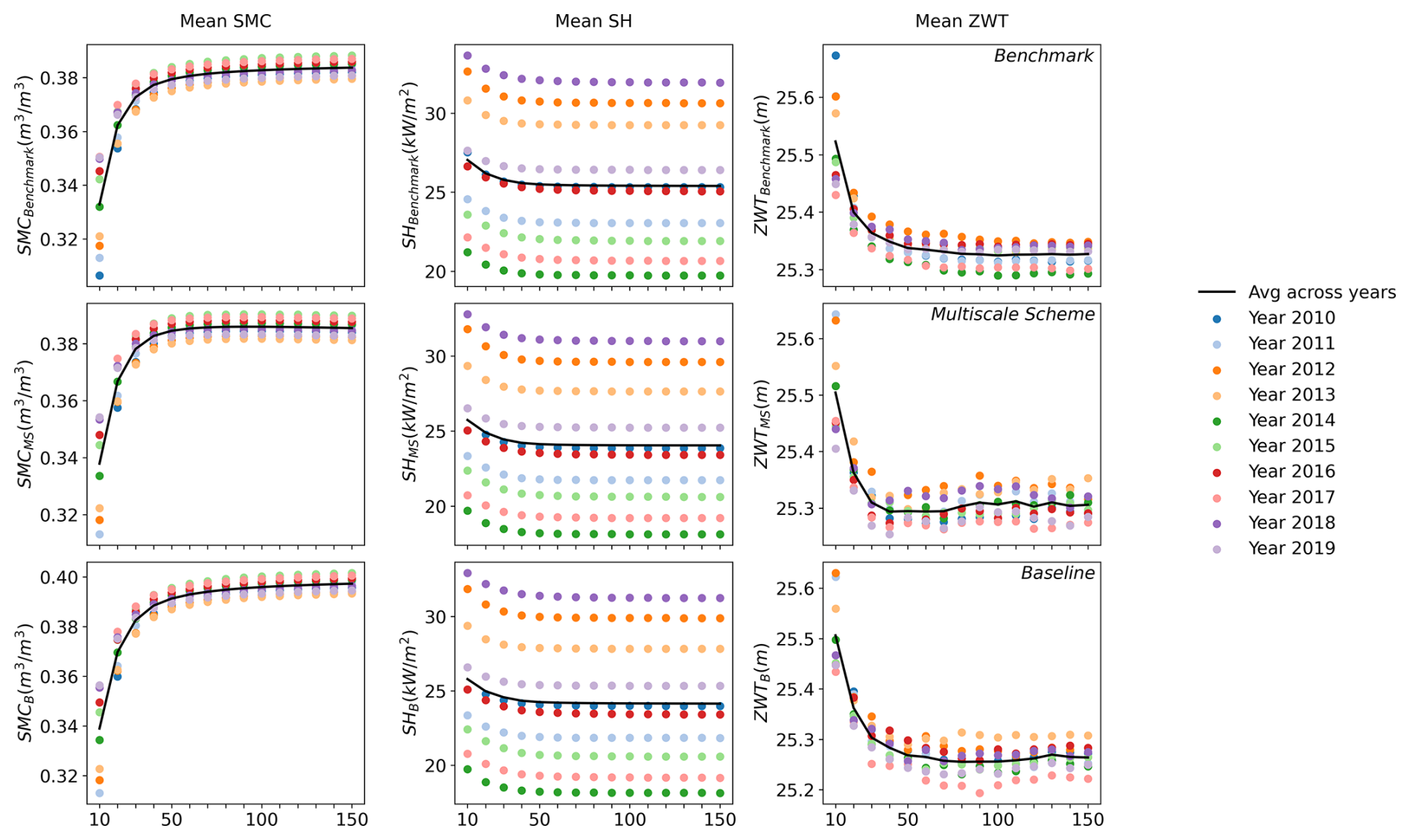
Figure 10 Comparison of spin-up for simulated spatial means of Soil Moisture Content (SMC), Sensible Heat Flux (SH), and Water Table Elevation (ZWT) between the multiscale scheme and benchmark simulation. The X-axis shows the total years of hourly simulations over a shared 10 year forcing period from 2010 to 2019.

The multiscale scheme shows minor fluctuations (typically less than 5 cm) during the final simulation decades, despite the clear convergence of SMC and SH. This dynamic equilibrium likely stems from how ZWT is defined and updated within the Noah-MP model; however, further analysis is necessary. In the employed SIMTOP scheme (see Sect. 2.3), ZWT is determined from soil water deficits and is highly sensitive to minor imbalances in the local surface water budget. Since it derives ZWT from storage dynamics rather than explicitly modeling groundwater flow, slight variations in soil moisture or lateral exchanges may induce minor shifts in the water table position. As a result, the long-term behavior reflects a steady state in which the water table fluctuates around a stable mean, rather than drifting toward a new equilibrium. The baseline experiment exhibits similar behavior. Nonetheless, the benchmark simulation does not display this variability. This is potentially due to the role the scale plays in defining the tiles for the two coarser experiments and to how heterogeneity is represented in both configurations.

Further analysis is needed to understand the differences between the Multiscale simulation and the Benchmark. Some HRUs may be overrepresented or underrepresented in the multiscale approach, resulting in discrepancies around the spatial mean. Coarser models average sub-grid changes over larger areas, which can overlook important dynamics or cause sudden variations. Additionally, significant numerical errors might occur from lateral flows affecting the overall water balance in the soil column, leading to abrupt changes in water content and noticeable oscillations.

2.6.1 Test Case under Homogeneous Conditions

Initially, controlled conditions were used to isolate the influence of elevation on subsurface flow, testing our hypothesis that the multiscale scheme will primarily show divergence flow patterns aligned with the topography.

For this experiment, variables, including land cover, soil properties, and meteorology, were homogenized across the 1°×1° domain to isolate the influence of elevation as the primary driver of subsurface flow. However, vertical heterogeneity remains between the layers of the soil column. This means that while each soil column within the domain's constituent tiles has uniform soil properties per layer, the properties differ between layers. This homogenization enables a focused evaluation of the new multiscale scheme's capability to represent water movement at various scales. Figure 11 shows the RISFUs used in this experiment and the saturated hydraulic conductivity map as an example of one of the homogenized parameters used.

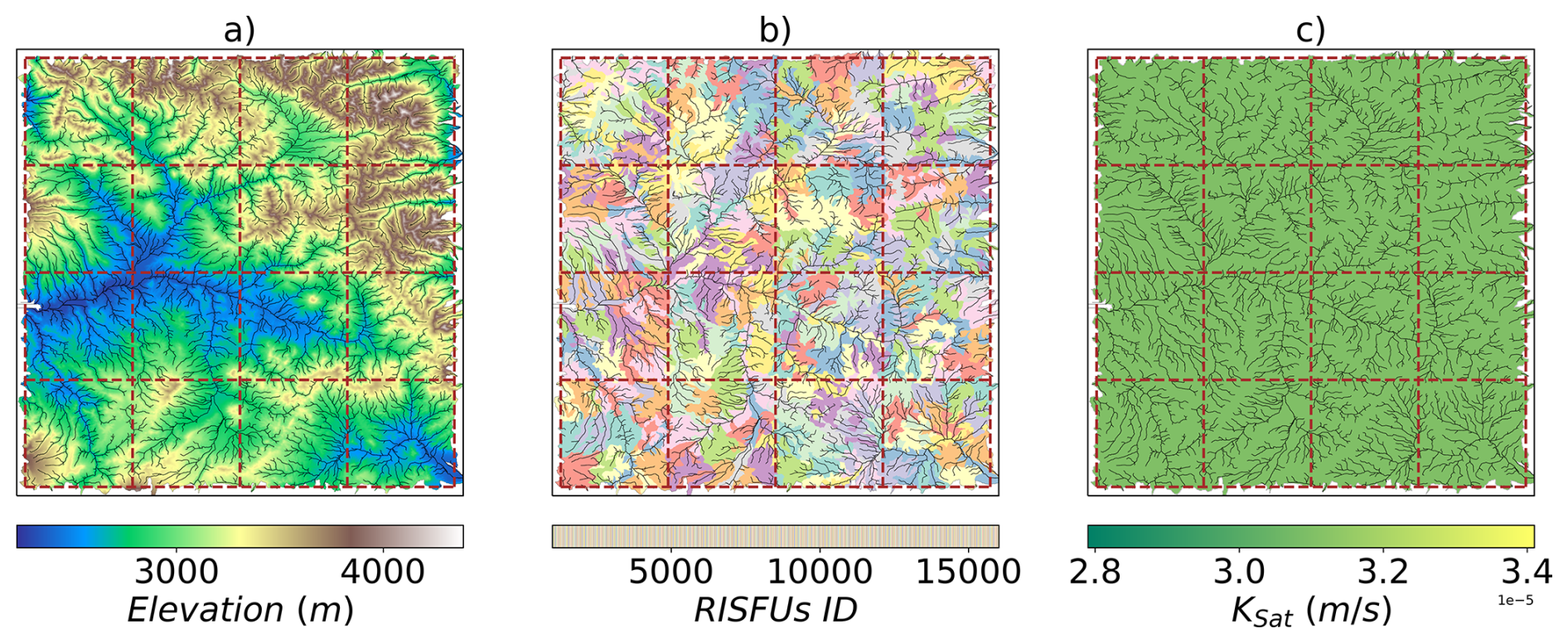
Figure 11 Regional and Intermediate Subsurface Flow Units (RISFUs). (a) Shows the elevation at ∼30 m scale resolution. (b) The RISFUs generated based on the cluster of watersheds (Fig. 9b), notice that each macroscale polygon has a total of 20 RISFUs. (c) Saturated Hydraulic Conductivity of the first layer of the soil column is presented as an example of the homogeneous soil hydraulic properties for all 40 700 tiles. Land cover and meteorological forcing data were also homogenized.

2.6.2 Test Case under Heterogeneous Conditions and Comparison against Baseline

The second part of this experiment introduces – layer by layer – the influence of small-scale heterogeneity from the land cover, soil hydraulic properties, and meteorological forcing variables to the homogeneous baseline presented in the previous section; this is, we returned each tile to its original parameters set to account for a more realistic effect on water absorption, retention, runoff, and infiltration.

Lastly, a comparison between our multiscale scheme and the baseline HydroBlocks identified differences in soil moisture, runoff, water table elevation, latent heat, and sensible heat.

2.6.3 Comparison of the Multiscale Scheme against a HydroBlocks Benchmark

We compared the outputs of the long-term simulation from the previous experiment (heterogeneous conditions) against a HydroBlocks benchmark. This benchmark consisted of 1.4 million tiles distributed among 64 parallel processes, as shown in Fig. 12. This configuration increased the number of tiles per macroscale polygon and the number of macroscale polygons, thereby capturing essential spatial heterogeneity and lateral subsurface interactions while remaining computationally feasible, given our computational constraints. The benchmark simulation also incorporated lateral interactions between the tiles located at the perimeters of each macroscale polygon, enabling water movement across the entire domain to capture regional and intermediate flow patterns.

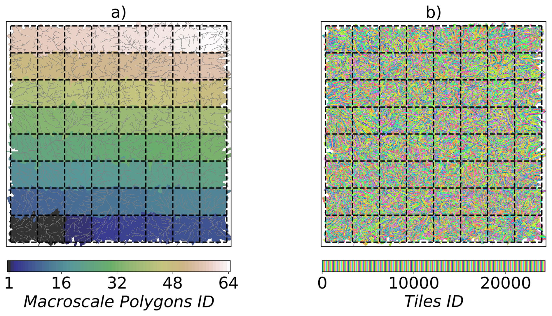
Figure 12 Benchmark setup. (a) The domain was divided into 64 macroscale polygons that were used to parallelize the LSM. (b) HydroBlocks HMC algorithm created approximately 1.4 million tiles to represent the spatial heterogeneity across the domain; each tile interacts laterally at the subsurface level with the neighboring areas within each macroscale polygon and with the tiles in the adjacent macroscale polygons if located in the perimeters.

Ideally, we would compare our simulations against a fully distributed model, where every grid cell of approximately 30 m resolution functions as its own tile (resulting in approximately 13 million tiles for the study area). However, due to the computational cost, simulating a 150 year-long hourly time series with such a detailed model was unfeasible with our available resources. Therefore, we opted for the highest number of tiles feasible within our limitations. The selected number of 1.4 million tiles represents 11 % of the number of tiles required for a fully distributed simulation.

3 Results

3.1 Test Case under Homogeneous Conditions

This section delineates the results of our experiments used to evaluate the new multiscale framework. Our primary objective is to assess the performance of the enhanced HydroBlocks framework, which incorporates regional, intermediate, additionally to the already implemented local lateral subsurface flow, and compare it to its baseline version, which only includes local.

The homogeneous experiment was run at an hourly time step for ten years. Under these controlled conditions, the multiscale framework was able to reproduce water movement between the RISFUs across and within macroscale polygons and among tiles of the same watershed following the topography, which was expected to be the first-order driver of subsurface flow.

Figure 13 summarizes the results for the one-year hourly average of the divergence flow computed for three different scales: regional, intermediate, and local; negative divergence values (in blue) indicate subsurface inflow and positive divergence values (in red) indicate outflow from the RISFUs and/or from the tiles.

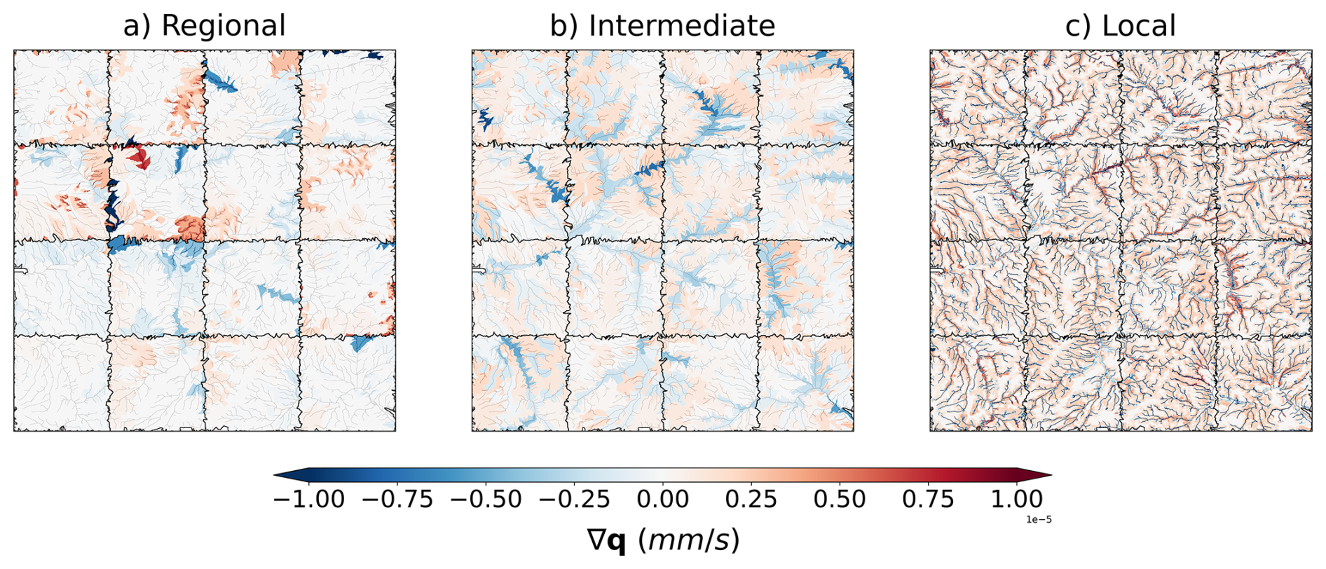
Figure 13 One-year average divergent subsurface flow under homogeneous soil hydraulic properties and meteorological forcing data, the blue color gradient indicates negative divergence (water gain), and the red color gradient indicates positive divergence (water loss). (a) Regional divergence of subsurface flow among RISFUs at the boundaries of the macroscale polygons. (b) Intermediate divergence subsurface flow among RISFUs within macroscale polygons in addition to the regional divergence from frame (a). (c) Local divergence subsurface flow among tiles within the same cluster of watersheds.

Regional subsurface flow: Fig. 13a illustrates the temporal mean divergence between RISFUs along the perimeters of macroscale polygons. Positive divergences are observed in higher elevation regions, indicating a net loss of water, whereas negative divergences in lower elevations suggest subsurface water gains across subdomains. This pattern aligns with the elevation map in Fig. 11a, as RISFUs account for the average elevation of the constituent tiles that, under homogeneous soil properties and meteorological forcing, lead to hydraulic heads in the soil column to resemble the topography.

Intermediate subsurface flow: Fig. 13b maps the average divergence among RISFUs within the macroscale polygons. The subsurface flow distribution occurs among RISFU units within each 0.25°×0.25° macroscale polygon. Consistent with Fig. 13a, elevation remains the primary driver of water movement, with higher elevations draining subsurface flow towards lower elevations, leading to flow accumulation near riparian zones.

Local subsurface flow: Fig. 13c presents the local subsurface flows, derived from the lateral interaction among tiles within the same watershed. The resultant divergence map clearly shows that stream area tiles accumulate water, while adjacent riparian zones exhibit water loss. Stream areas and riparian zones proximal to the main river also show greater water accumulation compared to ridge areas within the contributing watersheds.

Based on this initial analysis, we conclude that the implemented multiscale scheme effectively models regional and intermediate water movement across the domain by considering only elevation heterogeneity, while still remaining compatible with process parallelization. This outcome highlights the effectiveness of the multiscale scheme in capturing the spatial dynamics of water redistribution for large-scale subsurface flow within the land surface model.

3.2 Test Case under Heterogeneous Conditions and Comparison against Baseline of HydroBlocks

Figure 14 shows the temporal average divergence of the subsurface flow (aggregated regional, intermediate, and local divergence) for the same domain in the three heterogeneous cases compared to the previous homogeneous scenario.

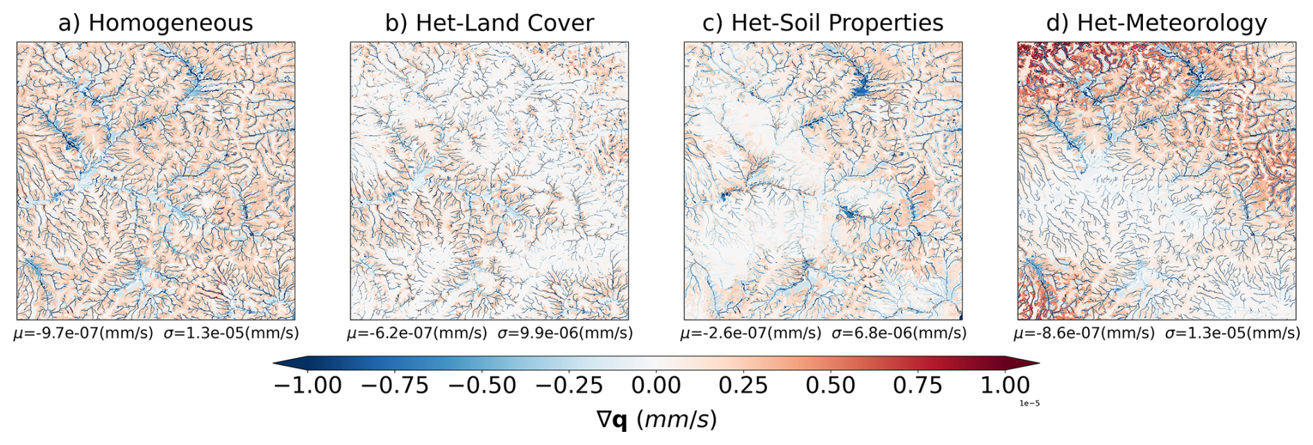
Figure 14 Time average divergent subsurface flow under heterogeneous conditions. (a) Subsurface flow under Homogeneous land cover, soil properties and meteorology (b) Subsurface flow under Heterogeneous Land cover. (c) Subsurface flow under Heterogeneous Soil hydraulic properties. (d) Subsurface flow under heterogeneous meteorological forcing variables (precipitation, wind, etc.).

• Heterogeneous Land Cover. The first layer of heterogeneity is introduced by the spatial variability of land cover. Figure 14b illustrates the computed divergence flow, where a change of ∼36 % in the mean is observed compared to the homogeneous case. This positive shift can be attributed to reduced runoff generation rates and enhanced water absorption in riparian zones due to vegetation.

• Heterogeneous Soil Properties. The second layer of heterogeneity consists of the spatially variable set of soil properties for each tile's soil column. Figure 14c shows a positive change in the mean of ∼73 %; primarily near the riparian zones, a reduction in the divergence is observed, indicating a slower contribution to subsurface flow rates. This is potentially due to the effect of soil texture, where soils with high water retention capacity slow down lateral water movement.

• Heterogeneous Meteorology. The final layer of heterogeneity is meteorology. Figure 14d displays a more pronounced pattern shift in subsurface flows compared to the homogeneous case, with higher rates of positive divergence near the north of the domain. In this instance, however, the change in the spatial mean is small (∼11 %), and the change in spatial distribution can be correlated to the pattern of total precipitation presented in Fig. 1. Higher divergence values are attributed to higher precipitation rates near the north of the domain and over the east-draining watersheds.

Contrary to Fig. 13, heterogeneity significantly influences local subsurface flow by affecting how water moves through and interacts with different soil layers, as evidenced in Fig. 14. Variations in soil properties, such as texture and permeability, impact water retention and infiltration rates. Land use and vegetation cover alter infiltration and evapotranspiration processes, while atmospheric conditions like precipitation and temperature affect the overall water budget in the soil column and runoff generation. Figure 15 differentiates the divergent subsurface flow between channels (a) and pixels in the high bands (b). Heterogeneous land cover reduces the subsurface flow reaching the channels approximately by 37 %, and soil properties by 70 %. In comparison, the high bands also experience an overall reduction of outflow of 44 %, which could be influenced by higher water uptake and evaporation due to vegetation cover. Similar behaviour is shown under the heterogeneous soil properties and meteorology experiments.

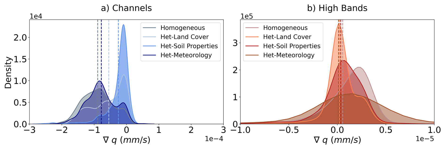
Figure 15 Distribution of divergent subsurface flow for streams (a) and high bands (b) showing the change in spatial mean (dotted lines) for the different heterogeneous scenarios.

As shown in Fig. 16, five output variables of the LSM were chosen to compute the differences against the baseline (only local lateral flow): soil moisture content (SMC), latent heat flux (LH), sensible heat flux (SH), surface runoff (R), and water table elevation (ZWT). The maps presented here represent the year-long hourly mean for the last year of a 150 year hourly simulation and are discussed below.

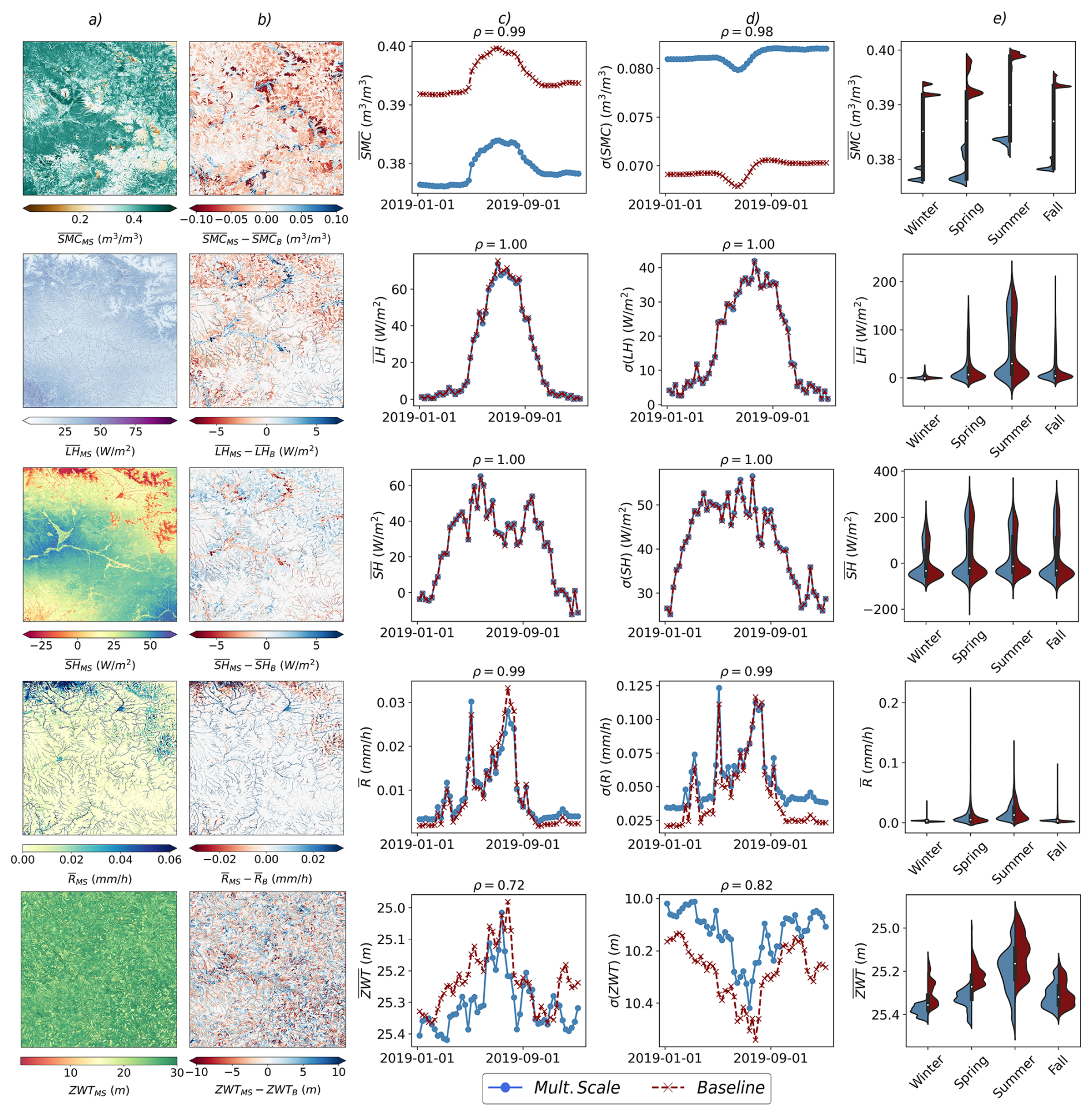
Figure 16 Comparison between the new Multiscale Scheme (MS) in HydroBlocks and the Baseline (B) for SMC, LH, SH, R and ZWT. Column (a) shows the spatial distribution of the time-averaged values for each variable from the MS. Column (b) displays the difference between the multiscale scheme and the baseline (MS-B). Columns (c) and (d) illustrates the weekly average time series of the spatial mean ($\stackrel{\mathrm{‾}}{X}$) and standard deviation (σ) of the last year of a 150 year simulation for each variable over the entire study domain. Column (e) shows the sesonality of the spatial mean.

Soil Moisture Content (SMC): Fig. 16 presents the map of averaged SMC from the multiscale scheme (column a). Compared to the baseline, the map (column b) reveals positive differences predominantly in the valley areas, while negative differences appear on the ridges. In some places, the RISFU used in the simulation can be identified as areas of uniform water gain or water loss. The time series of the spatial average for the last year of simulation shows the overall reduction in SMC while still capturing the temporal variability. Similarly, the spatial standard deviation follows the temporal dynamics, and it is further confirmed when comparing the distribution of SMC for each season. The latter shows an overall reduction in SMC.

The observed positive differences in valley areas can be attributed to saturated soils in the lowlands due to a redistribution of flows throughout our new scheme. In contrast, the negative differences on the ridges are due to faster drainage and reduced water retention, as these elevated areas are more prone to water loss. The uniform patterns of water gain and loss in the RISFU areas highlight the influence of regional to intermediate hydrological processes and soil characteristics for those particular spatial structures.

Latent and Sensible Heat Flux (LH/SH): The Latent and Sensible Heat Flux maps presented in Fig. 16 (column a) follow a similar pattern to that of SMC. In areas with relatively high subsurface flow, more water is available near the surface for evaporation, increasing the latent heat flux. Conversely, as more water moves through the soil, carrying heat with it, either cooling or warming the soil and altering the temperature gradient between the surface and the air, sensible heat flux decreases or increases, respectively.

Valley areas in the domain experience a positive difference in latent heat flux (and a comparable negative difference in sensible heat flux) due to the relatively higher soil moisture levels than the baseline. Subsurface flows can be more limited on ridges due to steeper topographic gradients. Consequently, the impact on latent and sensible heat fluxes is less pronounced in these areas, where higher temperatures and lower soil moisture levels prevail. However, recharge areas can be identified near streams, often occurring at relatively higher elevations than the locations they ultimately drain into.

The temporal variability of the spatial average for both energy fluxes closely matches that of the baseline (refer to column c) in Fig. 16. This strong correlation is primarily attributed to the dominant processes occurring in the superficial soil layers, which directly affect evaporation and heat exchange with the atmosphere. These layers respond rapidly to changes in atmospheric conditions and exert a significant influence on both components of the energy budget. In contrast, while subsurface flow redistributes soil moisture and heat within deeper layers, its impact on surface energy fluxes is less pronounced. Changes in moisture and heat within deeper layers take longer to propagate to the surface, and their effects are attenuated by the overlying soil layers.

Surface Runoff (R): Compared to the baseline, the multiscale scheme shows a positive difference in surface runoff for streams in lower elevation areas. This suggests more consistently saturated conditions resulting from contributing subsurface flow from riparian zones and higher elevation watersheds, as shown in columns (a) and (b) of Fig. 16. A distinct pattern is observed in the north of the domain, where higher total precipitation lead to higher flow rates in the streams immediately downstream. In contrast, for the major rivers in the central part of the domain, the impact on runoff generation is relatively dampened due to the influence of dominant regulatory processes (i.e., reduced precipitation and lower infiltration rates due to higher clay content). In this region, meteorological factors play a more significant role in runoff generation, as evidenced in Fig. 14c. The time series presented in column (c) and (d) of Fig. 16 illustrates the higher runoff generation, but and overall preservation of the sesonality.

Water Table Elevation (ZWT): The multiscale scheme simulates a consistently lower water table elevation across much of the domain, as shown in columns (b)–(e) of Fig. 16. This difference is especially pronounced in upland areas, where finer-scale lateral redistribution reduces local saturation by allowing water to drain more effectively toward downlospe tiles. Despite the lower overall water table, the seasonal signal remains well-preserved, indicating that the scheme stills captures the main meteorological controls and reflects a more realistic partitioning of water across the landscape, highlighting the role of topographic-driven lateral flow. This provides an indication that the new scheme facilitates drainage from elevated regions while concentrating moisture in convergence zones.

3.3 Approximation to the benchmark simulation

The outputs of the long-term simulation from the previous experiment, which involved heterogeneous conditions, were compared against a HydroBlocks benchmark. This benchmark consisted of 1.4 million tiles distributed into 64 parallel processes. We compared the long-term hourly mean for the last year of our 150 year simulation of the five output variables: SMC, LH, SH, R, and ZWT. Figure 17 shows both the multiscale scheme in column (a), the benchmark simulation in column (b), and a difference map [(a)−(b)] in column (c). For each variable, the mapped temporal mean shows a reasonable agreement between the results of the multiscale scheme and the benchmark simulation regarding variable range and spatial pattern distribution, as evidenced by the similarity in spatial mean ($\stackrel{\mathrm{‾}}{X}$) and spatial standard deviation (σ).

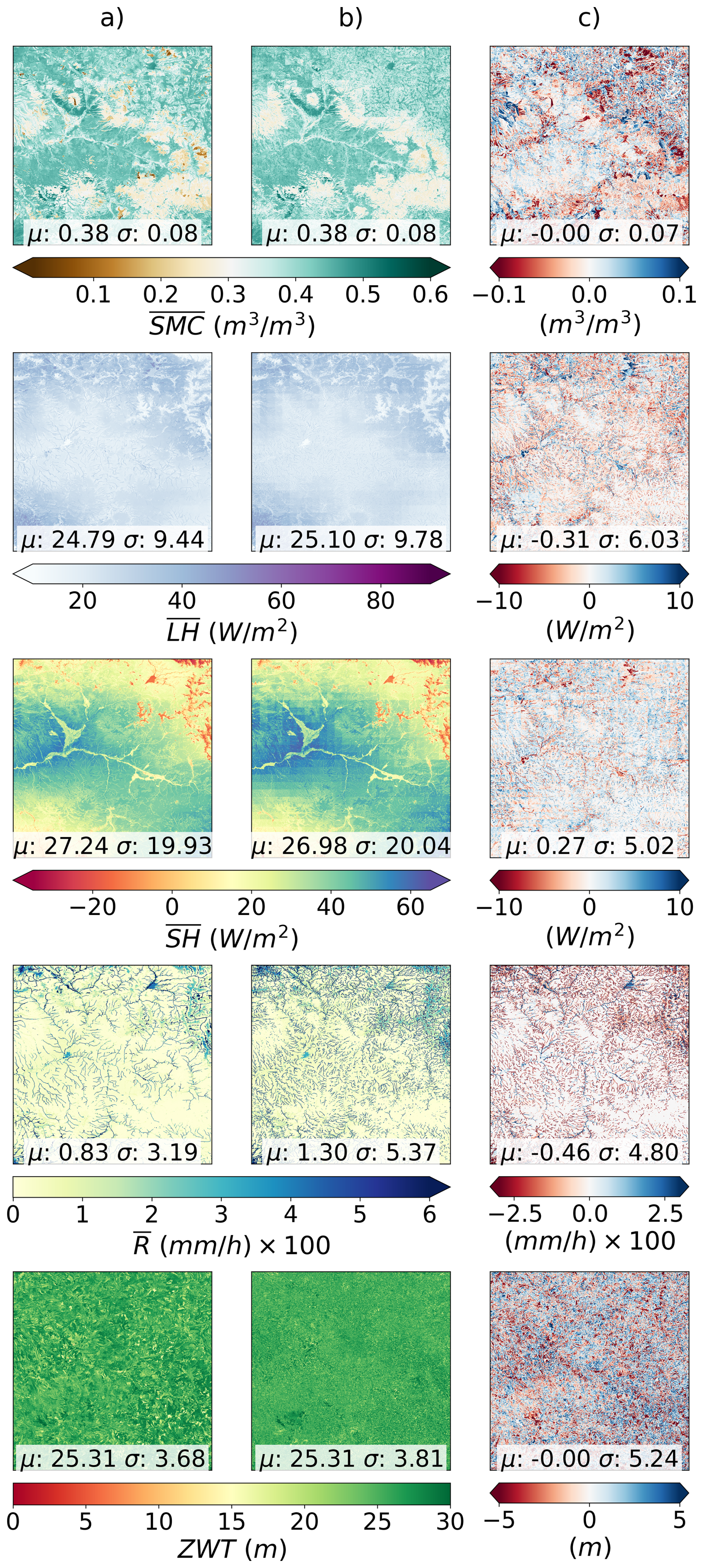
Figure 17 Output comparison of HydroBlocks Multiscale Scheme with 40.700 tiles (column a) and benchmark simulation with 1.4 million tiles (column b). The spatial fields of SMC, LH, SH, R, and ZWT are hourly averages of the one-year-long output time series. Column (c) shows the difference (a)−(b). The grid-like pattern in maps of column (b) is attributed to the imprint of the meteorological forcing dataset at $\mathrm{1}/\mathrm{32}$° resolution compared to domain subdivision at $\mathrm{1}/\mathrm{64}$°. μ and σ represent the spatial mean and standard deviation of the domain.

The benchmark simulation more accurately captures the fine-scale structure and dynamics of SMC, R, and ZWT. Stream channels and riparian features are clearly identified in the maps, reflecting the benchmarks' ability to resolve localized gradients and hydrological connectivity. In contrast, the multiscale scheme represents water redistribution over coarse units, which can blur small-scale heterogeneity. At finer resolution, the model can better represent convergent zones and lowland areas where subsurface flow will tend to accumulate; these flow pathways are smoothed out in the coarser simulation. Despite its coarser structure, the multiscale scheme still preserves the dominant seasonal patterns, as will be shown in Fig. 18, demonstrating that large-scale dynamics are maintained. However, the benchmark simulation offers a more physically realistic representation of how water is stored and released across the landscape.

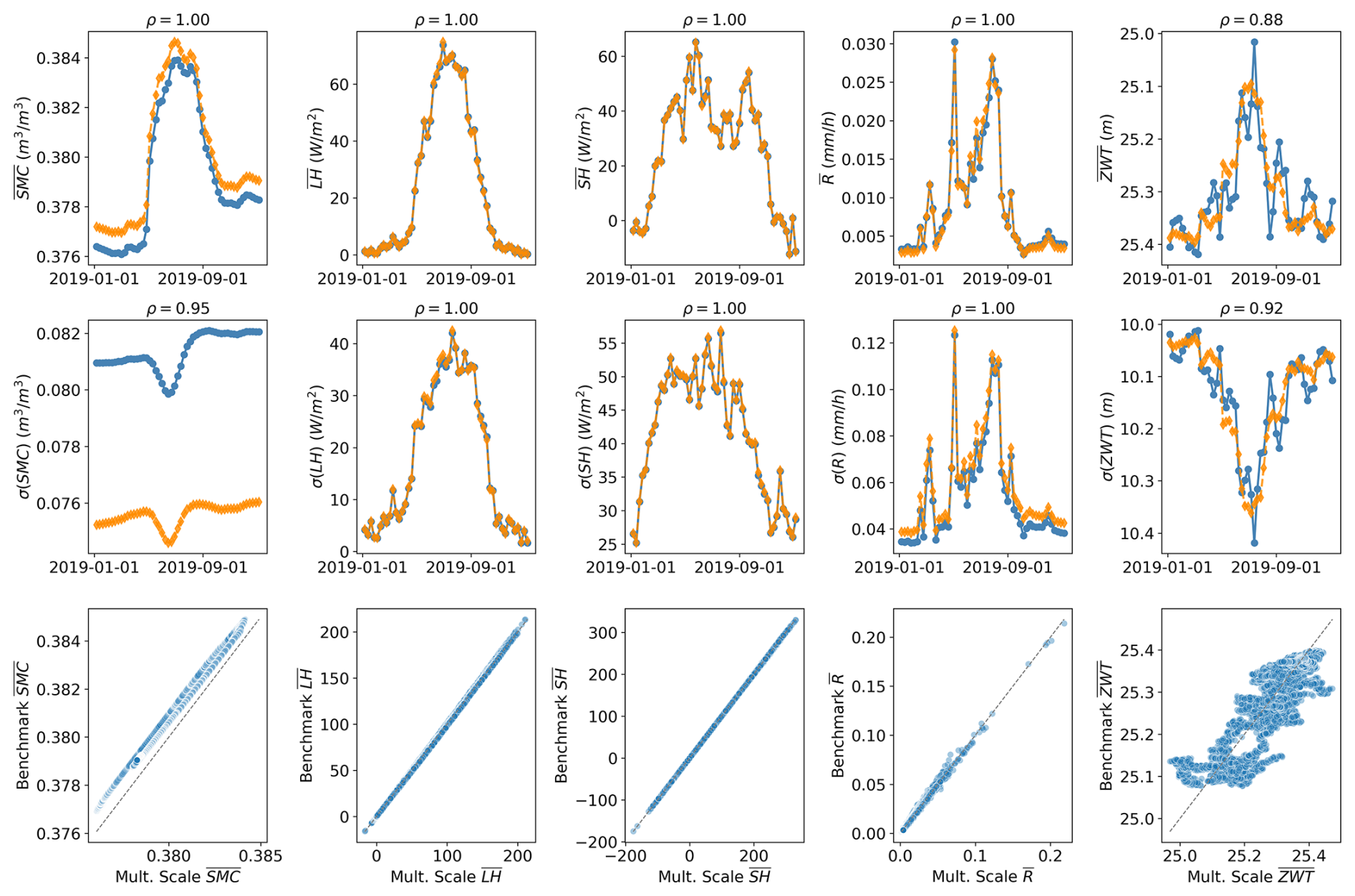
Figure 18 Temporal variability of the spatial mean ($\stackrel{\mathrm{‾}}{X}$) and standard deviation (σ) fields for SMC, LH, SH, R, and ZWT. In blue is the multiscale scheme time series; in orange are the results of the benchmark simulation. ρ is Pearson's correlation coefficient.

To further assess the performance of the multiscale scheme relative to the benchmark simulation, Fig. 18 presents a comparison of the daily averages of the spatial mean and standard deviation for output variables. The results indicate a strong overall agreement in the temporal variability of SH and LH between both models, as demonstrated by high Pearson correlation coefficients for both the mean and standard deviation time series. However, there are small yet evident discrepancies associated with the total water budget in the soil column as shown by the SMC, R, and ZWT time series.

The multiscale scheme differs from the benchmark by <1 % in spatial mean and in standard deviation, around 8 % from the R generated in the benchmark, and 7 % in SMC. In the case of LH and SH, the temporal mean values closely align between the two simulations, indicating consistency in large-scale water balance representation. However, the discrepancies in SMC and R are further accentuated when comparing ZWT, in which the multiscale scheme shows larger variability. This could be explained by the finer representation of spatial heterogeneity in elevation due to the higher resolution of the benchmark.

This increased variability further confirms the discrepancies observed in the spatial distribution maps shown in Fig. 17. The benchmark provides a more detailed representation of streams and river networks than the coarser simulation.

At this stage of analysis, a persistent difference between the two simulations can be observed, which is likely attributed to the representation of small-scale topographic heterogeneity in the benchmark simulation and a damped heterogeneity in the Multiscale Scheme due to coarser tiles. These differences indicate that the way elevation variability is represented might not be equally captured by the current tile-based configuration in both models. To further investigate these differences, we analyzed the temporal variability of SMC at two different depths of the soil column.

Figure 19 presents a comparative analysis of SMC at two levels: the root zone (0–0.05 m) and the bottom of the soil column (7–10 m). At the root zone level, there is a strong agreement between the multiscale scheme and the benchmark simulation, evidenced by a high Pearson correlation coefficient for both the mean and spatial standard deviation values. This close alignment suggests that the model effectively captures the dynamic processes occurring within the root zone, where soil moisture fluctuations respond rapidly to external influences such as root water uptake, evaporation, and precipitation events.

Figure 19 Temporal variability of the spatial mean ($\stackrel{\mathrm{‾}}{X}$) and standard deviation (σ) fields for SMC at root zone (top row) and bottom of the soil column (bottom row).

However, at deeper soil levels, substantial differences are introduced in both the mean ($\stackrel{\mathrm{‾}}{X}$) and spatial standard (σ) deviation values. These discrepancies highlight the challenges associated with modeling deeper soil layers. In these deeper layers, the effects of elevation become increasingly significant, influencing water distribution and movement. Unlike the root zone, where near-surface processes primarily drive water flow, deeper layers are subject to more diffuse and less direct flow paths, with hydraulic gradients influenced by subtle variations in elevation that may not be equally represented in both models. The effect of aggregating subsurface heterogeneity can also explain the differences between the two simulations, where the finer discretization allows water to percolate differently and could reproduce saturated areas better, producing more runoff, even if both models agree on superficial volumetric water content.

The benchmark simulation may predict a distribution of states, resulting in a more homogenized spatial distribution of subsurface flows instead of a single representative state for the equivalent of a single tile. These findings emphasize the importance of improving the representation of elevation heterogeneity in the tiling approach for both simulations to ensure a more robust validation of the multiscale scheme.

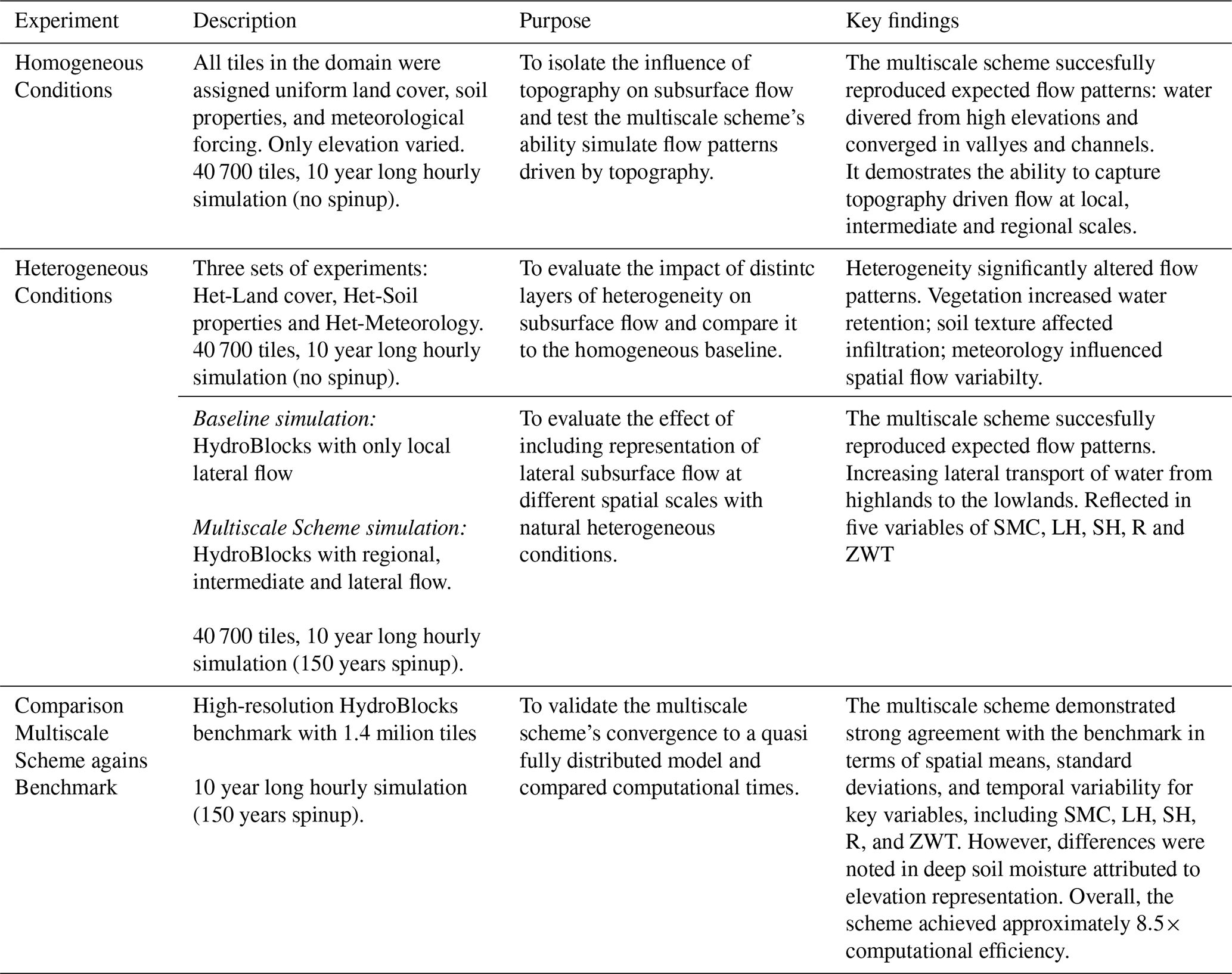
To synthesize the outcomes of our analysis, Table 1 provides a summary of the three core experiments conducted in this study. Each experiment evaluates the performance of the proposed multiscale scheme under varying conditions, ranging from idealized homogeneous setups to fully heterogeneous scenarios, and finally, a comparison against a high-resolution benchmark. This summary outlines the objectives, configurations, and key findings of each experiment to highlight the overall impact of our proposed methodology.

Table 1 Summary of the core experiments conducted to evaluate the HydroBlocks-MSSUBv0.1 multiscale lateral subsurface flow scheme.

4 Discussion

4.1 Advanced Subsurface Flow Simulation in LSMs Using the HydroBlocks Model

This study introduced a new scheme for simulating subsurface lateral flow in LSMs at local, intermediate, and regional scales, leveraging a novel and efficient tiling framework within the HydroBlocks LSM model. This approach aims to address the underrepresentation of subsurface flow paths between neighboring watersheds that could influence small-scale hydrological processes within large-scale domains while leveraging high-spatial and temporal resolution data and preserving computational efficiency.

The results of this study show a clear difference between the enhanced HydroBlocks simulation using the proposed multiscale scheme and the baseline case. These differences showcase the advantages of our approach to represent the multiple scales required for a more comprehensive simulation of the subsurface dynamics and potentially the groundwater system.

As this is a proof of concept, we aimed to isolate and better understand the effects of lateral flow parameterized across spatial scales. For the same reason, our validation strategy is designed to test internal model consistency rather than performance against external observations. Specifically, we validated our multiscale implementation against a quasi-fully distributed version of the same domain. This comparison allows us to evaluate whether the proposed approach can replicate hydrological patterns without the computational burden of resolving fine-scale lateral connectivity everywhere.

However, assessing the computational scalability and optimal setup of the multiscale approach over large regions, such as CONUS or even global areas, is essential for broader application. A major advantage of the current scheme is that it is designed for implementation in parallel computing systems. The lateral interaction among regional and intermediate subsurface flow units introduced here can be easily implemented to exploit the benefits of parallel simulations, and it can be scaled up to accomplish continental-scale simulations following the same principles for inter-domain communication. An idea that is not new and that has already been implemented in the routing scheme in HydroBlocks (Chaney et al., 2021), allowing for a more integrated hydrological system. Despite not being used in this study, HydroBlocks is capable of simulating channel flow across macroscale polygons and inter-domain communication. This capability highlights future directions for evaluating the impact of regional and intermediate subsurface flow on surface water distribution at the field scale, addressing a common problem in representing local processes influenced by regional groundwater dynamics.

Ongoing work focuses on applying and fine-tuning the multiscale scheme over larger domains, including a successful implementation over the Connecticut River Basin, which has enabled us to start examining scaling behavior and how it interacts with the river routing scheme.

4.2 Parameterization Challenges and Validation in Multiscale Hydrological Modeling

Although not the focus of this study, it is essential to acknowledge the uncertainties associated with the datasets used, which can potentially lead to biases in model predictions when compared to actual observations. Additionally, as the resolution of the model increases, an inherent uncertainty is introduced to the model processes due to the extensive requirements for model parameterization (Beven et al., 2015; Bierkens et al., 2015). We compared the spatial and temporal variability of generated time series of soil moisture content, latent and sensible heat flux, as well as runoff generation and water table elevation, with a more discretized solution (benchmark) of our test domain using HydroBlocks, for a 150 year hourly simulation. Our validation shows agreement between the multiscale scheme and the benchmark in terms of spatial mean, standard deviation, and Pearson's correlation coefficient; this highlights the capacity of our scheme to capture seasonal variability and average spatial dynamics while still preserving computational efficiency. When considering the parameterization of the LSM, the proposed approach relies on the redistribution of soil moisture in the vertical soil column and the lateral flow between them, driven by a modeled hydraulic gradient; such characterization of the soil column and land surface properties obeys a single realization of the datasets presented in Sect. 2.1. However, a sensitivity analysis of the parameters could lead to a more comprehensive understanding of its role in the subsurface dynamics to approach a closer representation of observed fields. This is important as models such as HydroBlocks, and consequently, the introduced multiscale scheme, permit thousands of simulations to explore parameter sensitivity and uncertainty quantification (Chaney et al., 2016).

One area of improvement for the current model structure is the representation of soil column depth. Our current assumption of a constant soil column depth of 10 m everywhere neglects groundwater flows occurring at greater depths. Importantly, this undermines the role of subsurface heterogeneity, as one would expect shallower vadose zones near the lowland and deeper in the upland. To address these issues, future work should focus on: (i) altering the parameterization to include variable soil column depths and rock structure involving detailed characterization of the vadose zone across different topographical features, and (ii) characterizing aquifer properties at high spatial resolutions, incorporating variations in hydraulic conductivity, porosity, and storage coefficients. This could be accomplished by integrating diverse datasets, including geological surveys, remote sensing data, and detailed soil surveys, to refine the model inputs and reduce uncertainties.

When validating high-spatial-resolution models at the macroscale, point-based observations often struggle to adequately capture the spatiotemporal dynamics of hydrological variables (Koch et al., 2015). Simultaneously identifying both spatial and temporal patterns is crucial, especially as the current generation of LSMs and computational resources advances toward more detailed representations of land surface dynamics (Koch et al., 2016; Torres-Rojas et al., 2024; Zink et al., 2018). These patterns are essential for validating distributed models and predictions by effectively capturing trends and anomalies in environmental data. For example, flooding dynamics are highly sensitive to local factors such as channel bathymetry, riverbed slope, and floodplain inundation, making extensive observations critical for validating water level dynamics. The launch of the Surface Water and Ocean Topography (SWOT) mission provides high-resolution (∼100 m) water surface elevation data, offering a unique opportunity to study flooding dynamics and enhance their representation in LSMs (Biancamaria et al., 2016; Pedinotti et al., 2014). By validating HydroBlocks against SWOT data, we could improve our understanding of the processes governing flooding dynamics and refine both LSM structures and spatially distributed validation strategies.

4.3 Balancing Efficiency and Accuracy in HydroBlocks Pseudo-3D Approach for Lateral Flow

The proposed multiscale methodology offers a flexible and computationally efficient approach to simulating subsurface hydrological processes in land surface models. By leveraging the tiling-based structure of HydroBlocks, the method enables large-scale simulations without the prohibitive computational costs typically associated with fully distributed models. For instance, a one-year benchmark simulation using the fully resolved 1.4 million tile configuration requires approximately 340 h on a single core. In contrast, the multiscale implementation reduces this time to 40 h, an 8.5-fold speedup, consuming only 12 % of the computational resources. For perspective, HydroBlocks without the multiscale formulation completes the same run in approximately 32 h, highlighting that most of the additional time comes from resolving lateral flow across scales.

However, some assumptions and limitations are inherent to this approach:

HydroBlocks employs a pseudo-3D numerical solution of Richards' equation, which decouples vertical and lateral water flow simulation to reduce computational complexity while preserving important dynamics (Chaney et al., 2021). Vertical flow is solved first in Noah-MP using an implicit scheme, which captures processes such as infiltration and root water uptake under both unsaturated/saturated conditions. Subsequently, lateral flow is computed based on the hydraulic gradient between adjacent soil columns (tiles) using Darcy's equation.

This operator-splitting approach, where vertical and horizontal processes are resolved sequentially, is widely used in land surface and hydrological models and assumes that vertical processes dominate in the unsaturated zone due to larger vertical gradients. While efficient, this decoupling introduces mass balance errors and is best viewed as a first-order approximation. Such errors can be particularly significant under conditions where vertical and horizontal gradients are strongly coupled, such as during rapid recharge events or in heterogeneous subsurface conditions.

When lateral fluxes are computed from coarser, depth-average heads, each tile represents an average state across potentially heterogeneous profiles. This could explain some of the differences between the benchmark simulation and the multiscale scheme. The lumping of heterogeneities produces an effective lateral transmissivity that may not correspond to the same small-scale hydraulic connections; therefore, the apparent lateral conductivity becomes scale-dependent as the tiles increase in size, the more diffuse the actual gradients, and lateral redistribution can be under- or over-represented depending on how averaging is done.

In the current scheme, Darcy's equation is applied to lateral flow in both saturated and unsaturated zones, with soil moisture-dependent hydraulic conductivity reflecting the nonlinear effects of saturation on subsurface connectivity. Although this generalization simplifies implementation, it does not explicitly differentiate between saturated and unsaturated domains in lateral flow computations. We consider that such differentiation can also limit physical interpretability, in particular in regions with complex stratigraphy, perched water tables, or shallow impermeable layers where saturation boundaries are spatially discontinuous.

The underlying decomposition assumes that vertical and horizontal flows occur on different time scales, with vertical flow being dominant in the unsaturated zone due to gravitational acceleration, and horizontal flow dominating in saturated layers due to capillary equilibrium. This generally holds in steep terrains or where soils remain relatively dry, but may not hold where horizontal pressure gradients become more prominent. In such cases, small horizontal gradients assumed in the model may underestimate lateral redistribution, particularly at depths where soil moisture variability is dampened and pressure gradients are primarily driven by elevation.

Additionally, the use of a quasi-steady state hydrostatic assumption linking soil moisture and water table depth allows for a simplified numerical solution. However, this assumption may be invalid under transient conditions, such as during rapid infiltration, snowmelt, or irrigation events.

Despite these limitations, the pseudo-3D approach remains practical for many large-scale applications where computational constraints are significant and fully 3D simulations become impractical. In many natural environments, such as agricultural systems or shallow aquifers, vertical processes like infiltration and root uptake occur much faster than lateral redistribution. In such settings, decoupling provides a good balance between process realism and model performance.

Future work should focus on extending the current operator-splitting framework to explore a more grounded separation of saturated and unsaturated domains in the soil columns and to address the numerical scale effects inherent to the pseudo-3D approach. This would involve solving lateral flow using Darcy's law exclusively in saturated zones, while maintaining vertical-only flow in unsaturated regions, in line with the common approach, implementing adaptive time coupling to reduce lag errors between vertical and lateral fluxes, developing scale-consistent upscaling methods for effective hydraulic parameters, and exploring implicit solutions to define the iterative exchanges within each time step. Evaluating the accuracy of such approaches through comparison with fully 3D Richards-based models would provide a valuable insight into the trade-offs between physical fidelity and computational efficiency. In addition, addressing the effects of scale to the pseudo-3D

4.4 Suitability of Unsaturated Lateral Flow in the Multiscale Scheme

LSMs commonly separate saturated from unsaturated soil layers when simulating lateral flow between soil columns, allowing horizontal flow only in the saturated zone and vertical flow primarily in the unsaturated zone (e.g., Hazenberg et al., 2015; Swenson et al., 2019; Xie et al., 2020). This approach stems from the differences in physical mechanisms: in saturated zones, groundwater can move laterally following potential gradients often modeled by Darcy's law; unsaturated zones, on the other hand, are dominated by capillary and adsorptive forces. Many models have adopted this scheme because it allows for practical analytical and numerical solutions, especially at larger scales, ensuring stability, computational efficiency, and easier mass conservation checks (Brandhorst et al., 2021; Zeng et al., 2019). At large scales, horizontal flow in the unsaturated zone could be considered negligible.

This separation is valid primarily for gently sloping areas where unsaturated lateral gradients are minimal. However, growing evidence from high-resolution studies and complex terrain modeling indicates that topographic/gravity and matric potential gradients substantially influence lateral flow under unsaturated conditions, causing soil water movements from high to low potential (Gannon et al., 2017; Luo et al., 2018; Zhou et al., 2023). The scientific community is increasingly pushing towards the inclusion of lateral unsaturated flow to capture better complex processes (e.g., Kim and Mohanty, 2016; Kong et al., 2016; Qiu et al., 2024), for example, studies by researchers like Lu et al. (2011) have shown that flow directions in isotropic, homogeneous unsaturated hillslopes can be simultaneously upslope, vertical, and downslope, demonstrating the significant role of the gradient of moisture content (matric potential) alongside gravity.

Restricting lateral flow to only the saturated zone limits model capacity in representing hillslope hydrology, where gravitational forces substantially influence unsaturated lateral flow, in simulating the formation of perched water tables, and lateral movement in the capillary fringe. At hyper-resolutions, the influence of local topography becomes more relevant (Ji et al., 2017). Spatial variability of soil moisture in the unsaturated zone cannot be described successfully without a relevant understanding of how the subsurface flow is distributed or connected vertically or laterally in complex landscapes.

Our experiments do not enforce a strict separation between saturated and unsaturated zones, thereby allowing flux exchange across these boundaries. In this case, flow is modeled according to Darcy's law, employing a moisture-dependent hydraulic conductivity that is computed as the harmonic mean of the conductivities of the interacting soil columns. The hydraulic gradient is formulated to incorporate both hydrostatic pressure head in saturated domains and matric potential in unsaturated domains, enabling representation of pressure-driven flow across a continuum of saturation states. The use of Darcy's law extended with a moisture-dependent conductivity is a simplifying convenience for conceptualizing unsaturated flow. In these unsaturated conditions, hydrostatic equilibrium fails because pressure and moisture gradients change dynamically as water moves.

Incorporating full lateral unsaturated flow enhances model realism, particularly where lateral drainage is controlled by topographic variations. This formulation is beneficial because it naturally reduces excessive subsurface runoff by allowing hydraulic conductivity to decrease drastically in dry soils. Ultimately, including this parameterization will enable models to describe the spatial variability of soil moisture in the unsaturated zone and capture critical phenomena such as wetting fronts (Dai et al., 2019) and the contribution of lateral flow to base-flow recession (Liang et al., 2017).

Our model aims to demonstrate a heuristic approach with cross-saturation flow, but can revert to the traditional LSM separation by allowing lateral interaction only between layers flagged as saturated. Although we intend to go beyond this constraint, implementing saturated-only lateral flow is straightforward through flow criteria adjustments. This, however, falls outside the scope of this study and requires dedicated analysis.

Future work should focus on systematically analyzing the error budget introduced by the lateral flow simplification across different spatial scales. This would involve running the model at different grid resolutions and tile configurations to identify the critical resolution threshold below which including lateral unsaturated flow is necessary for a more physically accurate simulation.

4.5 Optimal Spatial Representation of Subsurface Structure in Hydrological Simulations

This study employs clusters of watersheds to define regional and intermediate modeling units, and during the experimental phase, watersheds were also tested, yielding similar results. However, when watersheds are used as modeling units, the spatial disconnection between tiles becomes problematic for accurately redistributing regional flow back to individual tiles, as one tile can belong to two different watersheds. Despite this limitation, the numerical solution and computational efficiency gained from this approach make it worthwhile. The model balances accuracy and processing speed by focusing on a simplified regional structure, enabling simulations at high spatial resolutions that would otherwise be computationally limited.

A critical and ongoing challenge is the lack of an established method for determining the optimal number and configuration of tiles necessary to adequately represent spatial heterogeneity in hydrologic processes across different scales. While tiling schemes offer flexibility, their effectiveness depends heavily on how well they balance computational cost with hydrological realism. Torres-Rojas et al. (2022) have previously addressed this issue by introducing a metric that helps identify the most effective parameter configuration for capturing important features of heterogeneity while reducing the computational cost of fully distributed simulations. Nevertheless, this remains an open area of research. Further studies are needed to develop scalable and generalizable strategies for tile configuration and, in our case, definition of regional/intermediate units that reflect the dominant hydrologic controls.

While the current tiling strategy simplifies the subsurface by associating it with surface-defined clusters of watersheds, this can limit the model's ability to simulate groundwater flow and storage. To better represent the subsurface structure, it is important to incorporate detailed geological and hydrogeological data into the model that reflects variations in subsurface features. This can enhance accuracy rather than relying solely on clusters of watersheds or individual watersheds as defining parameters for the subsurface structure. This involves integrating information about varying soil types, rock formations, and aquifer properties to more precisely capture the spatial variability in hydraulic conductivity, porosity, and other key parameters for groundwater flow.

Incorporating these detailed subsurface characteristics allows for a more realistic simulation of groundwater flow and interactions between different layers of soil and rock. This enhanced representation helps address the limitations of assuming a constant distance to bedrock or treating regional units as a replica of superficial water divisions.

As shown in Sect. 3.3: Approximation to the benchmark simulation, the influence of topography over lateral water redistribution between tiles is highly dependent on the tile configuration. Addressing the challenges associated with optimal spatial representation of land surface heterogeneity is required. Moreover, the optimal tile configuration is model-dependent, and one could prioritize subsurface heterogeneity over surface heterogeneity in natural settings where groundwater dynamics is the major driving mechanism; this is clustering based on soil properties and elevation.

4.6 Scale decomposition in the Multiscale Scheme

This paper introduces a multiscale decomposition of subsurface processes designed to manage complexity and reduce the computational burden of simulating field-scale hydrology across large to continental domains. Rather than relying on fixed natural boundaries, this approach aligns hydrological processes with their characteristic spatial scales, creating a structured approximation that enables efficient and physically meaningful simulations.

The scale separation is informed by a process-based rationale:

• Local scale. Captures fine-scale heterogeneity in topography, land cover, and soil properties, which are critical for infiltration, runoff generation, and soil moisture redistribution.

• Intermediate scale. Represents dominant lateral flow pathways within clusters of hydrologically similar watersheds. These units enable the physical redistribution of water within bounded lateral areas, typically within macroscale polygons that resemble grid cells in ESMs.

• Regional scale. Subsurface flow moves across macroscale polygons by the lateral connectivity between RISFU units at the boundaries. Defined to divide the domain into multiple parallel processes (e.g., ∼25 km) and serve as the upper boundary for subsurface lateral exchange.

This decomposition establishes a flexible framework that is not tied to a specific resolution. If higher-resolution atmospheric forcing becomes available, the regional units can be refined accordingly, and the intermediate and local structures adapt hierarchically within each smaller domain. On the other end, coarser atmospheric grids (e.g., 50–250 km) can also be accommodated by aggregating the regional units while preserving internal multiscale structure.

Importantly, the numerical implementation supports arbitrary shapes and configurations of the regional and intermediate units as long as consistent topological relationships (e.g., adjacency) are provided. Lateral fluxes are computed in a generalized form that supports irregular areas. However, the shape and size of these units may influence the realism of lateral flow, especially near domain boundaries or in regions with strong directional gradients, and merit further investigation.

Ongoing work is exploring the sensitivity of surface and subsurface responses to the configuration of the RISFUs, including the influence of meteorological forcing resolution, polygon shape, and internal variability within each scale.

5 Conclusions

This study evaluates the potential of using a tiling scheme to represent regional and intermediate flow paths using HydroBlocks LSM. The LSM enables the high-resolution simulation of water and energy fluxes within the landscape. The proposed methodology comprises the definition of parameterized regional and intermediate subsurface flow units using the soil hydraulic properties of the tiles within each unit to define the dynamic movement of water between soil columns. Soil hydraulic properties such as soil moisture content, saturated and residual water content, and hydraulic conductivity are crucial for accurately simulating water flow. The experiment adopts a constant soil column depth and resolves the vertical water movement using Noah-MP as part of the HydroBlocks framework.

The current approach adopts a cluster of watersheds configuration for the regional and intermediate modeling units to represent the subsurface structure. It defines the lateral interaction between them across subdomains to exploit the advantages of parallel computing systems. This configuration mimics natural hydrological boundaries, ensuring water flow simulation across different regions.

The current study demonstrates the potential of the tiling scheme within a defined domain. It also lays the path to implementing this multiscale scheme at continental scales, which requires addressing boundary conditions across domains to reflect the continuity of subsurface flow paths and the influence of large natural hydraulic drivers, such as lakes and oceans, on regional groundwater dynamics.

Due to computational limitations, the methodology is compared against a quasi-fully distributed solution of HydroBlocks of 1.4 million tiles. This benchmark simulation allows for detailed spatial representation while balancing computational efficiency, making it a suitable benchmark for comparison. The multiscale scheme converges to the benchmark in spatial mean and standard deviation, as well as temporal variability, indicating the potential, robustness, and accuracy for simulating regional hydrological processes. However, more work is required to validate the proposed methodology, as the elevation heterogeneity representation in both models differs considerably, and the benchmark simulation appears to better resolve lateral water redistribution, resulting in higher soil moisture content and runoff generation relative to the multiscale schemes.